Safety Performance Function for Motorways using Generalized Estimation Equations

Procedia - Social and Behavioral Sciences 53 ( 2012 ) 901 – 910

1877-0428 © 2012 The Authors. Published by Elsevier Ltd. Selection and/or peer-review under responsibility of SIIV2012 Scientifi c Committeedoi: 10.1016/j.sbspro.2012.09.939

SIIV - 5th International Congress - Sustainability of Road Infrastructures

Safety Performance Function for motorways using Generalized Estimation Equations

Salvatore Cafisoa*, Carmelo D’Agostinoa aDepartment of Civil and Environmental Engineering, University of Catania, Viale Andrea Doria 6, 95125 Catania, Italy

Abstract

Accident prediction models (APMs) are useful tools for estimating the expected number of crashes over a road network which are typically used in the screening of sites with promise for safety improvements. This study shows a procedure of analysis for motorways network offering a comparison between the conventional analytical techniques based on GLM (Generalized Linear Model) and a different approach based on GEE (General Estimating Equation). The GEE model, incorporating the time trend, is compared in terms of results and reliability in the estimation with conventional models (GLM) that do not take into account the temporal correlation of accident data. © 2012 The Authors. Published by Elsevier Ltd. Selection and/or peer-review under responsibility of SIIV2012 Scientific Committee Keywords: Safety Performance Function; Generalized Estimation Equation; Generalized Linear Model.

1. Introduction

The process of identification of hazardous locations in a given road itinerary is a key step to increase significantly the safety level of that route, for this purpose, it must be the most accurate and detailed as possible and should result in a list of sites that can be defined as "high risk" and therefore characterized by a high potential for improvement in terms of reducing the number of accidents and / or their severity [1].

The countermeasures to be implemented in a road network to maximize safety can be manifold, from the most simple and inexpensive to complex and radical. One of the criteria on which often the Transportation Engineering

* Corresponding author. Tel.: +39-095-7382213; fax: +39-095-7382247. E-mail address: [email protected]

Available online at www.sciencedirect.com

© 2012 The Authors. Published by Elsevier Ltd. Selection and/or peer-review under responsibility of SIIV2012 Scientific Committee

902 Salvatore Cafi so and Carmelo D’Agostino / Procedia - Social and Behavioral Sciences 53 ( 2012 ) 901 – 910

base to decide if and what improvements to adopt to the network (or where to place these) is analyzing the number and location of accident in recent years. This method has the limitation of being tied to strong fluctuations of random accidents, in the sense that if a place has been several accident recently, this will not mean that they occur others in the same place. This is why it should use procedures with more of the theoretical foundations, taking into account other aspects [2] [3].

Accidents count observed at a site (road segment, intersection, interchange) is commonly used as a fundamental indicator of safety performing road safety analysis methods. Because crashes are random events, crash frequencies naturally fluctuate over time at any given site. The randomness of accident occurrence indicates that short term crash frequencies alone are not a reliable estimator of long-term crash frequency. This year-to-year variability in crash frequencies adversely affects crash estimation based on crash data collected over short periods. The short-term average crash frequency may vary significantly from the long-term average crash frequency. This effect is magnified at study locations with low crash frequencies where changes due to variability in crash frequencies represent an even larger fluctuation relative to the expected average crash frequency. When a period with a comparatively high crash frequency is observed, it is statistically probable that the following period will be followed by a comparatively low crash frequency. This tendency is known as regression-to-the-mean (RTM), and also is evident when a low crash frequency period is followed by a higher crash frequency period.

Failure to account for the effects of RTM introduces the potential for “RTM bias”, also known as “selection bias”. Selection bias occurs when sites are selected for treatment based on short-term trends in observed crash frequency. RTM bias can also result in the overestimation of the effectiveness of a treatment (i.e., the change in expected average crash frequency). Without accounting for RTM bias, it is not possible to know if an observed reduction in crashes is due to the treatment or if it would have occurred without the modification. In light of what has been said the safety level of a site can not be simply defined by its accidents history. Generalizing it can be said that the safety of an element of a road must be defined by the average expected number of accidents in a long period of time.To this aim, the use of longer periods of observation would be more appropriate. In general, this period of analysis depends on the availability of both traffic and crash data, but in literature numerous studies have shown that periods longer than 5 years of investigation could reduce the accuracy in the estimation of the Safety Performance Function as they introduce the natural time trend that with the traditional analysis technique using generalized linear models (GLM) can not be taken into account. This phenomenon is very pronounced in the motorway sector, as accident rate is very low if compared to the urban or rural highways and a typical period of analysis that is enough on other contexts is not sufficient. If it is possible to have several years of analysis, however, can take into account the annual variation or trend in the calibration of SPFs due to the influence of factors which change over time using the General Estimating Equation (GEE) that incorporates time trend [4] In order to assess this variation, the number of accidents of each year is treated as a single observation. Unfortunately, this procedure generates the disaggregation of data by creating a temporal correlation that can not be identified with conventional procedures of model calibration using GLM.

Basing on the previous considerations, the objective of this paper is to illustrate the application of the GEE procedure to traffic-safety studies when several years of data are available and when it is desirable to incorporate trend. The application is for a segment of a Motorway in Sicily, Italy, using data for the years 2003 through 2009. The GEE models with trend are compared with GLM that do not account for temporal correlation in the accident count data. It is necessary, first, to provide some background on accident modeling before introducing the GEE concept.

2. Methodological remarks

Crash observed at a site i in the year t (Yi,t) are typical time series data across years and can, therefore, be represented by the following simplified model structure:


Yi,t = trend + regression term + random effects + local factors where “trend” refers to a long-term movement due to a change in the risk factors with time, the “regression

term” is of the same form as the Safety Performance Functions (SPF), “random effects” accounts for latent variables across the sites, and the “local factors” refers to the dispersion between the normal safety level for similar locations and the safety level for the specific site. This last term indicates the effects of local risk factors and also general factors that are not included in the safety performance function. Random effects and local factors both contribute to the dispersion of crash counts as compared to the mean value estimated by the regression term.

The use of the Negative Binomial (NB) distribution to represent the distribution of crash counts is commonly accepted. Therefore, excluding trend effects (i.e. the phenomenon is stationary) GLMs are especially useful in the context of traffic safety, for which the distribution of accident counts in a population often follows the negative binomial distributions [5] [6].

The important property of the GLM is the flexibility in specifying the probability distribution for the random component [7] [8] [9].

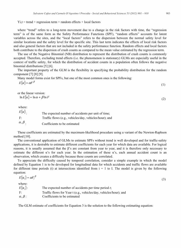
Many model forms exist for SPFs, but one of the most common ones is the following: { } βακ FE = (1)

or the linear version:

{ } FE lnlnln βακ += (2)

where: { }κE : The expected number of accidents per unit of time;

F: Traffic flows (e.g., vehicles/day, vehicles/hour); and βα , : Coefficients to be estimated

These coefficients are estimated by the maximum-likelihood procedure using a variant of the Newton-Raphson

method [10]. The conventional application of GLMs to estimate SPFs without trend is well developed and for traffic-safety

applications, it is desirable to estimate different coefficients for each year for which data are available. For logical reasons, it is usually assumed that the ’s are constant from year to year, and it is therefore only necessary to estimate the different ’s for each year. In the estimation of these ’s, each annual accident count is an observation, which creates a difficulty because these counts are correlated.

To appreciate the difficulty caused by temporal correlation, consider a simple example in which the model defined by Equation 1 is to be developed for longitudinal data for which accidents and traffic flows are available for different time periods (t) at intersections identified from i = 1 to I. The model is given by the following equation:

{ } βακ tt FE = (3) where:

{ }tE κ : The expected number of accidents per time period t; F: Traffic flows for Year t (e.g., vehicles/day, vehicles/hour); and

βα , : Coefficients to be estimated The GLM estimate of coefficients for Equation 3 is the solution to the following estimating equation:


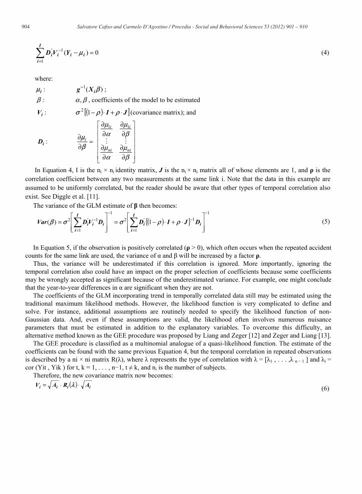
0)(1

1' =−=

−I

iiiii YVD μ (4)

where:

iμ : )(1 βiXg− ; β : βα , , coefficients of the model to be estimated

iV : ( )[ ]JI ⋅+⋅− ρρσ 12 (covariance matrix); and

iD : =∂∂

βμi

∂∂

∂∂

∂∂

∂∂

βμ

αμ

βμ

αμ

nini

ii 11

In Equation 4, I is the ni × ni identity matrix, J is the ni × ni matrix all of whose elements are 1, and is the correlation coefficient between any two measurements at the same link i. Note that the data in this example are assumed to be uniformly correlated, but the reader should be aware that other types of temporal correlation also exist. See Diggle et al. [11].

The variance of the GLM estimate of then becomes:

( ){ }1

1

1'21

1

1'2 1)(−

=

−−

=

− ⋅+⋅−==I

iii

I

iiii DJIDDVDVar ρρσσβ (5)

In Equation 5, if the observation is positively correlated ( > 0), which often occurs when the repeated accident

counts for the same link are used, the variance of and will be increased by a factor . Thus, the variance will be underestimated if this correlation is ignored. More importantly, ignoring the

temporal correlation also could have an impact on the proper selection of coefficients because some coefficients may be wrongly accepted as significant because of the underestimated variance. For example, one might conclude that the year-to-year differences in are significant when they are not.

The coefficients of the GLM incorporating trend in temporally correlated data still may be estimated using the traditional maximum likelihood methods. However, the likelihood function is very complicated to define and solve. For instance, additional assumptions are routinely needed to specify the likelihood function of non-Gaussian data. And, even if these assumptions are valid, the likelihood often involves numerous nuisance parameters that must be estimated in addition to the explanatory variables. To overcome this difficulty, an alternative method known as the GEE procedure was proposed by Liang and Zeger [12] and Zeger and Liang [13].

The GEE procedure is classified as a multinomial analogue of a quasi-likelihood function. The estimate of the coefficients can be found with the same previous Equation 4, but the temporal correlation in repeated observations is described by a ni × ni matrix R( ), where represents the type of correlation with = [ 1 , . . . , n 1 ] and i = cor (Yit , Yik ) for t, k = 1, . . . , n 1, t k, and ni is the number of subjects.

Therefore, the new covariance matrix now becomes: ( ) iiii ARAV ⋅⋅= λ (6)


where Ai is an ni × ni matrix with diag [V(μi1 ), . . . V(μiTi )]. The covariance matrix is given by Equation 7:

1

1

1'2)ˆcov(−

=

−=I

iiii DVDσβ (7)

One can find the solution by simultaneously solving Equations 6 and 7 with the iterative reweighted least-

squares method [10]. This method is required because the estimates of both and need to be found. To solve the GEE correctly, every element of the correlation matrix Ri has to be known. However, in many

instances, it is not possible to know the proper correlation type for the repeated measurements. To overcome this drawback, Liang and Zeger [12] proposed the use of a “working” matrixV̂ of the correlation matrix Vi which is based on the correlation matrix iR̂ . The estimate of the coefficients is found with the following equation:

0)(ˆ1

1' =−=

−I

iiiii YVD μ (8)

The covariance matrix of Equation 9 is given by:

( )1

1

1'

1

11'1

1

1'2 ˆˆˆˆˆcov−

=

−

=

−−−

=

−=I

iiii

I

iiiiii

I

iiii DVDDVVVDDVDσβ (9)

The proposed methodology in Equations 8 and 9 possesses one very useful property in that β̂ nearly always

provides consistent estimates of even if the matrix Vi has been estimated improperly. Thus, the confidence interval for will be correct even when the covariance matrix is specified incorrectly. Therefore, it is not necessary to, a priori, examine the type of temporal correlation (e.g., independent, dependent). Techniques on how to analyze and interpret autocorrelation can be found in books on time-series analysis such as those by Box and Jenkins [14] and Diggle [15]. One important drawback, however, comes with this property. To assume that β̂ is the proper estimate of , it is required that the observation for each subject be known and available. If missing values exist, the estimate of the coefficients may be biased. The extent of the bias is influenced by the type of missing values (e.g. random or informative). Note that, in the case of ii VV =ˆ

, Equation (9) becomes the covariance matrix of Equation (7).

3. SPF calibration

The SPFs proposed in this work are basically of two types. The first are based on the application of a model which the only explanatory variables are the Annual Average Daily Traffic (AADT) and the segment length (L) (exposure variables), while the second class of models in which in addiction to the exposure variable there are a series of other variable depending to the physically characteristic of the road segment (multivariable models). Both classes of models will be analyzed using both Generalized Linear Model (GLM) and Generalized Estimating Equation (GEE). With the use of the latter finally the data is analyzed by incorporating in the model time trend.

The general form of SPF is shown in equation 10:

( ) =×××=

m

iii xb

a eAADTLeYE 11α (10)

where: xi: generic additional variable, m: number of generic additional variable,


, a1, bi: m +2 regression parameters.

The estimate will be zero if only at least one of the exposure variables (L and AADT) assumes a zero value. With regard to the model depending only on the traffic shall be considered null the additional xi and it is taken into account only the length of segment and AADT. The application of the proposed safety performance function is performed on segments of the A18 CT-ME from the years 2003 to 2009 excluding 2004 because during year 2004 the Agency has adequate safety barriers in different parts of infrastructure changing the homogeneity of the segments within the year of analysis. The whole dataset consists of 652 segments of variable length and more than 70 m. Accident take into account are fatal and injury, for an amount of 451 accident in six years of analysis. Segmentation was carried out to maintain all the variable constant within each segment. The choose (of the threshold of 70 m) to have segment longer than 70 m comes out from a balance between the number of residual accidents, after the elimination of shorter segment and the problem related to an appropriate statistical inference.

In the case of multivariable models the APM assumes the form:

( ) dqaRSHaViadaRilaGdaCurvaaa eAADTLeYE t ⋅+⋅+⋅+⋅+⋅+⋅+ ×××= 76543210 α (11)

where: Curv, Gd, Ril, Viad, RSH dq: additional variable,

t: the additional factor which take into account time trend, a0, a1, a2, …, a7: 8 regression parameters. To each of them are associated all the information necessary for the application of the multivariable models that are:

• The Roadside Hazard (RSH), which assumes 6 possible values (from 1 to 6, in increasing order of potential hazard), defined as follows: first, we consider only the conditions of the outer margin, assigning 1 to the trench, 2 embankment with appropriate barriers, 3 to the viaduct with adequate lateral barrier, 4 embankment with the side dam is not adequate, 5 to the viaduct with adequate lateral barrier, and then this value is the sum 1 in the case in which the median barrier is not to norm. This parameter is variable over time, due to maintenance and replacement of the barriers made by the Agency. In particular, it is changed from 2004 onwards in viaduct;

• The slope of the grade downhill (Gd), this variable is significant in that it influences the speed of heavy vehicles and therefore determines the average speed of flows. It assumes the value zero in the uphill and assumes the value of the slope of the segment when it is down;

• The lack of cross slope of the sections analyzed (dq), analytically defined as the difference between the cross slope required according to the new Italian standard taking into account the radius of curvature and the type of road and what detected in situ;

• The variables related to the type of section (RIL and VIAD), are variables of type exclusive. They report the status of the homogeneous section. Those that were statistically significant are embankment and viaduct is instead discarded the trench. Therefore the variables described above assume the value 1 in the sections where it is embankment or viaduct and 0 in other segments;

• The variable relating to the curvature of the homogeneous road element (Curv) defined as the actual curvature of each element.

4. Results

The application of the models leads to the results shown in Table 1. These coefficients were estimated using the SAS software linearizing the equation and reporting for each estimated coefficient the standard error and for each


model the relative dispersion parameter. The dispersion parameter represents the error in the construction of the model and is estimated by an iterative procedure using SAS software package. The models are all over 6. The first two were calibrated using the GLM in particular the multivariate model is the model 1 and the second (model 2) is the basic model in which the only independent variable are AADT and L. The model 3 and 4 were calibrated with GEE taking into account the time trend. In particular, model 3 is the multivariate and model 4 depends only of AADT and L. Finally, models 5 and 6 were calibrated using the GEE but not considering the time trend. Comparing the results obtained by evaluating the standard error and the value of the coefficients of the regression is shown as the model 1 and model 2 have identical coefficients respectively to the models 5 and 6. This is due to the fact that the dataset used to calibrate is identical for all models. What varies is the value of the standard error of coefficients which is generally greater in models calibrated with GEE. Underestimating the standard could have an impact on the proper selection of coefficients because some coefficients may be wrongly accepted as significant because of the underestimated variance.

On the other hand if dispersion parameter is considered, it is noted that for the classes of models calibrated not considering the time trend both they are calibrated using the GLM than the GEE it is identical. This again depends on the fact that the database used is the same.

If instead of it is compared the models with the time trend calibrated with GEE (models 3 and 4) with those that do not take into account time correlation it is evident that the time trend also intervene on the value of the coefficients of all variables in the model. This is explained by the fact that the database used for the calibration while being identical, it is interpreted by the GEE model as a repetition of the various segments for each year of analysis and that it varies in both the traffic that some of the considered parameters.

In general, the models which do not consider time trend analyzes used the database as whole do not taking into account the repetition of the segment in different years, therefore, considering a larger sample than model with time trend of t times where t is the number of years of analysis. This is the reason for the lower value of dispersion parameter in models that incorporate temporal trends than the other. In practical terms, analyzing the results reported in Table 1, we can say that with the traditional models (models 1, 2, 5, 6) that incorporate temporal trends would underestimate the expected number of accidents in the years 2003, 2006 and 2007 while we overestimated the value of the 2005 expected number of accidents, all related to last year of analysis. Referring to the dispersion parameter, has to be noted that difference in the estimation of the dispersion parameter can produce different results when the Empirical Bayes procedure is applied [16].

4.1. Model validation

The goodness of fit of the models generated was investigated using the method of cumulate residuals (CURE), i.e. the sum of the differences between the number of accident observed at a site and the expected value at the same site in the same year. As the residuals of all models are normally distributed with expected value equal to 0 and variance equal to [17], it is possible to calculate the variance of the expected value of such site as the square of the cumulate residuals. The purpose is to evaluate the variance of the system and the trend of the variation of AADT residuals in order to identify any abnormal deviations of the SPF used and evaluate how it fits to the dataset. The following figures show the cumulate residuals for the proposed models (Figure 1).

The advantage of the method CURE is that it is independent from the number of observations, which is the case with other methods on the goodness of fit of models [18]. Analyzing the graphs it can be concluded that, as expected, the multivariable models (1, 3, 5), even if it is plotted respect only AADT oscillates much more close to zero and tend to exceed the limits of 2 only in the proximity of the ends. Further consideration should be made on the peaks of cumulate residuals for multivariable models. Indeed, in the multinomial model that consider temporal trends (3) both the positive and negative peaks of the cumulate residuals are generally smaller than in multi models that not incorporate temporal trends (1 and 5) showing a better fit of the model to the dataset. Finally


also the lower amplitude of the oscillation of the residuals around the axis of abscissas indicates a lower dispersion of the residues to vary AADTs for multivariable models.

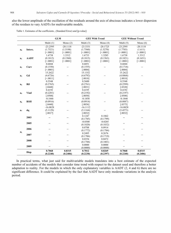
Table 1. Estimates of the coefficients , (Standard Error) and [p-value]:

GLM GEE With Trend GEE Without Trend

Multi (1) Mono (2) Multi (3) Mono (4) Multi (5) Mono (6)

a0 Interc. -23.2595 (1.7521) [<.0001]

-20.1118 (1.5198) [<.0001]

-23.3331 (1.7560) [<.0001]

-20.1725 (1.5270) [<.0001]

-23.2595 (1.7703) [<.0001]

-20.1118 (1.611)

[<.0001]

a1 AADT 1.6738

(0.1812) [<.0001]

1.3312 (0.1560) [<.0001]

1.6733 (0.1815) [<.0001]

1.3285 (0.1563) [<.0001]

1.6738 (0.1821) [<.0001]

1.3312 (0.1651) [<.0001]

a2 Curv 0.6044

(0.1550) [<.0001]

-- 0.6051

(0.1555) [.0004]

-- 0.6044

(0.1718) [.0004]

--

a3 Gd 15.2622 (4.6726) [<.0011]

-- 15.1352 (4.6792) [.0018]

-- 15.2622 (4.8868) [.0018]

--

a4 Ril 0.5548

(0.2765) [.0448]

-- 0.5600

(0.2761) [.0031]

-- 0.5548

(0.2599) [.0328]

--

a5 Viad 0.4192

(0.2201) [.0500]

-- 0.4195

(0.2192) [.0050]

-- 0.4192

(0.2197) [.0500]

--

a6 RSH -0.1846 (0.0916) [.0440]

-- -0.1858 (0.0914) [.0036]

-- -0.1846 (0.0887) [.0375]

--

a7 dq -16.0828 (5.1129) [.0017]

-- -16.1112 (5.1164) [.0032]

-- -16.0828 (5.4573) [.0032]

--

t

2003 -- -- 0.1247 (0.1785)

0.1062 (0.1799) -- --

2005 -- -- -0.0300 (0.1820)

-0.0205 (0.1832) -- --

2006 -- -- 0.0788 (0.1772)

0.0914 (0.1784) -- --

2007 -- -- 0.2495 (0.1706)

0.2676 (0.1719) -- --

2008 -- -- 0.0354 (0.1788)

0.0472 (0.1801) -- --

2009 -- -- 0.0000 (0.0000)

0.0000 (0.0000) -- --

Disp. 0.7068 (0.2240)

0.8315 (0.2406)

0.7012 (0.2230)

0.8269 (0.2397)

0.7068 (0.2240)

0.8315 (0.2406)

In practical terms, what just said for multivariable models translates into a best estimate of the expected

number of accidents of the models that consider time trend with respect to the dataset used and therefore a better adaptation to reality. For the models in which the only explanatory variables is AADT (2, 4 and 6) there are no significant difference. It could be explained by the fact that AADT have only moderate variations in the analysis period.


(a) (b)

(c) (d)

(e) (f)

Fig. 1.Cure plot with ±2 for: (a) model 1, (b) model 2, (c) model 3, (d) model 4, (e) model 5 and (f) model 6.

5. Conclusion

In the present paper were six different APMs have been analyzed, two of which incorporate temporal trends in the calibration of models with the use of GEE. The remaining four APMs were calibrated using basic and multivariable models by the way of classical GLM and GEE without trend. The data used are relative to a section of motorway A18 for a total of 652 segments and considering a period of analysis from 2003 to 2009 with the exclusion of 2004. The purpose of the paper was to investigate the accuracy of different models that incorporate temporal trends respect to the classical models which do not take into account the temporal correlation of crash data. The time trend models were calibrated with the use of SAS software for which a script was created ad hoc by which it was possible to generate models that have a different constant value depending on the year of analysis. In this way it is possible capture the variations in the expected number of accidents of sites investigated, due to the time correlation, compared to a year of analysis included in the time period analyzed. Analyzing the results it can be stated that the time correction generates a better goodness of fit of models that incorporate temporal trends. It also corrects over-underestimation of the standard errors of the regression coefficients and of the dispersion parameter obtained by the more traditional GLIM approach. This results, even if derived by the example application on an Italian Motorway, are consistent with other studies [4] [19]. Improving accuracy in the


calibration of regression parameters and standard errors improve the quality of the SPMs and lead to more refined results when the EB approach is used to control the phenomenon of regression to the mean. Another advantage is related to the possibility of using a broader period of analysis. In fact, GEE that incorporate temporal trends are not affected by the extension of the period of analysis for two reasons. The first is that the data are analyzed as repetitions of the variables in different years and therefore although this reduces the size of the sample, makes sure that the analyst can use more years of analysis. The second is that the temporal correlation that is generated between the sites in different years does not generate errors related to the type and size of the correlation matrix used in the calibration of the model and this allows to insert all the years available. This characteristic is useful especially when long period of observations are needed to increase the sample size or to carry our before/after studies. In contrast, the calibration of the models with GEE is critical in case of missing value and therefore requires a quality and detail of data higher than the traditional techniques [4].

Nomenclature

E(Y) expected annual crash frequency of random variable Y;

AADT average annual daily traffic [vehic/d];

L length of road segment [m];

References

[1] AASHTO (2011). Highway Safety Manual, pp. 105-106, Washington, D.C., USA. [2] Cafiso, S., Di Silvestro, G., Persaud, B., Begum, M.A. (2010). Revisiting variability of dispersion parameter of safety performance for two-lane rural roads.,Transportation Research Record, Vol. 2148, pp,38-46. [3] Cafiso, S., Di Silvestro, G. (2011). Performance of safety indicators in identification of black spots on two-lane rural roads, Transportation Research Record. Vol. 2237,pp. 78-87. [4] Lord, D. and Persaud, B. N. (1998). Accident Prediction Models With and Without Trend Application of the Generalized Estimating Equations Procedure. In Transportation Research Record, No. 1717. [5] Kulmala, R. (1995). Safety at Rural Three- and Four-Arm Junctions: Development and Applications of Accident Prediction Models. VTT Publications 233, Technical Research Centre of Finland. [6] Nicholson, A. and Turner, S. (1996). Estimating Accidents in a Road Network. In Proceedings of Roads 96 Conference, Part 5, New Zealand, , pp. 53–66. [7] Dunlop, D. D. (1994). “Regression for Longitudinal Data: A Bridge from Least- Squares Regressions”. The American Statistician, Vol. 48, No. 4, , pp. 299–303. [8] McCullagh, P. and Nelder, J. A. (1989). Generalized Linear Models: Second Edition. Chapman and Hall, Ltd., London. [9] Myers, R. (1990). Classical and Modern Regression with Applications. Duxbury Press, Belmont, U.K.. [10] Green, P. (1984). Iterative Reweighted Least Squares for Maximum-Likelihood Estimation and Some Robust and Resistant Alternative (with discussion). Journal of the Royal Statistical Society, Series B, Vol. 46, pp. 149–162. [11] Diggle, P. J., Liang, K.-Y. and Zeger, S. L. (1994). “Analysis of Longitudinal Data”. Clarendon Press, Oxford, U.K.. [12] Liang, K.-Y. and Zeger, S. L. (1986). Longitudinal Data Analysis Using Generalized Linear Models. Biometrika, Vol. 73, , pp. 13-22. [13] Zeger, S. L. and Liang, K.Y. (1986). Longitudinal Data Analysis for Discrete and Continuous Outcomes. Biometrics, Vol. 42, pp.121-30. [14] Box, G. P. and Jenkins, G. M. (1970). Time-Series Analysis: Forecasting and Control (rev. ed.). Holden-Day, San Francisco, California. [15] Diggle, P. J. (1990). Time Series: A Biostatistical Introduction. Oxford University Press, Oxford, U.K.. [16] Hauer, E. (2001). Overdispersion in modelling accidents on road sections and in Empirical Bayes estimation. Accident Analysis & Prevention, Vol. 33, No. 6,. pp. 799-808. [17] Hauer, E. and Bamfo, J. (1997). Two Tools for Finding What Function Links the Dependent Variable to the Explanatory Variables. In Proceedings of ICTCT Conference, Lund, Sweden. [18] Miaou, S.-P. (1996). Measuring the Goodness-of-Fit of Accident-Prediction Models. Report FHWA-RD-96-040. FHWA, McLean, Va.. [19] Giuffrè O., Granà A., Giuffrè T., Marino R. (2007), Improving Reliability of Road Safety Estimates based on High Correlated Accidents Counts. Transportation Research Record, No. 2019, 2007.

Documents

Safety Performance Function for Motorways using Generalized Estimation Equations