Safe Mud Pump Management While Conditioning … a methodology that is used in an automatic drilling control system ... (especially with oil -based mud) ... Safe Mud Pump Management

Safe Mud Pump Management while Conditioning Mud:

On the Adverse Effects of Complex Heat Transfer and Barite Sag when

Establishing Circulation

Eric Cayeux*

*International Research Institute of Stavanger, Stavanger, N-4068,

Norway (Tel: +47 51 87 50 07; e-mail: [email protected]).

Abstract: For complex drilling operations with narrow geo-pressure windows, it is not uncommon to

have problems with formation fracturing, due to erroneous mud pump management. To assist the driller

in managing the circulation, it is possible to limit both the acceleration of the mud pumps whilst changing

the flow-rate as well as the actual flow-rate, to avoid generating downhole pressure above the fracturing

pressure gradient of the open hole section. Such mud pump operating limits are dependent on the

operational parameters (e.g. drill-string axial and rotational velocities), and the in situ conditions

downhole. The in situ conditions evolve with time due to the changes of bit and bottom hole depths as

well as the variations in temperature, mud properties and cutting concentrations. When starting to

condition mud after a long period of time without circulation, the changes in temperature can be very

large. Furthermore, in the eventuality of barite sag, lifting up drilling fluids containing a large

concentration of high gravity solid can cause much increase of the downhole pressure. This paper

presents a methodology that is used in an automatic drilling control system to account for all those factors

in order to have a safe mud pump management including circumstances where mud is being conditioned.

Keywords: drilling automation, safe guard, physical model, mud pump management, mud pump

acceleration, maximum flow-rate, formation fracturing gradient, mud losses, barite sag, heat transfer.

1. INTRODUCTION

An excessive mud pump acceleration or a too large flow-

rate can generate downhole pressures that exceed the

fracturing pressure gradient of the open hole formation

therefore causing mud losses and in the worst case scenario, a

loss circulation incident. The maximum tolerable pump

accelerations and flow-rates are very context dependent

(Iversen et al. 2009). Both the drilling operational parameters

and the downhole conditions dictate the well safe guards to

be used. When drilling is well established, the time

dependence of those limits is mostly influenced by the

change of depth. But while conditioning mud after a long

period of time without mud circulation, the downhole

conditions change quickly because of the combined effect of

heat exchange happening with the cold fresh mud being

pumped into the well and the displacement of the mud in

place which properties may have been altered during the

period of inactivity. This paper describes an automatic system

that attempts at enforcing mud pump safe guards that adapt

themselves to the current downhole conditions.

2. AUTOMATION OF MUD PUMP MANAGEMENT

In this section, we will first describe the fundamental

physical characteristics of the drilling hydraulic system and

then we will present the method used to solve the problem of

managing the mud pumps during a drilling operation.

2.1 Drilling hydraulics

In conventional drilling and with a simple drill-string and

BHA (Bottom Hole Assembly), the drilling hydraulic system

is composed of two branches connected together at the level

of the bit: the drill-string branch and the annulus branch (see

Fig. 1). Note that if the bit is off bottom, the annulus branch

is longer than the drill-string one.

Fig. 1: The drilling hydraulic system can be seen as a

network of interconnected branches.

But several junction points may exist, if there are

components like circulation-subs, hole openers, under-

reamers, downhole motors, etc. in the drill-string because

such elements provides access from the inside of the drill-

string to the annulus at other places than the bit. The result is

a network of inter-connected branches. The condition to be

respected by this network is that the pressures on both sides

of the junction point between the two branches are equal.

Proceedings of the 2012 IFAC Workshop on AutomaticControl in Offshore Oil and Gas Production, NorwegianUniversity of Science and Technology, Trondheim,Norway, May 31 - June 1, 2012

FrAT1.4

Copyright held by the International Federation ofAutomatic Control

231

To describe the behaviour of the drilling fluid in each

branch we can use a cross sectional averaging of the Navier-

Stokes equation (Fjelde et al., 2003). There are three balance

equations that describe the interface exchange of mass,

momentum and energy.

The mass balance can be written:

( )

( ) (1)

where is time, is the curvilinear abscissa, is the cross-

sectional area of a fluid element, is the averaged density,

is the average velocity, is the source term, a mass per

length per time through the fluid element side walls.

In a multi-phase context, it is more complicated to write

the momentum balance. The assumption made here is to use a

drift-flux formulation where the different phases are mixed

together but each phase has a slip velocity compare to a

reference one. The momentum balance can then be written as

follow:

( )

( )

( ( ))

(2)

where is the pressure, is the friction pressure-loss term,

is the average inclination of the fluid element, is the

gravitational acceleration of the earth.

Finally, the energy conservation can be written (Marshall

and Bentsen, 1982):

( ) ( ) , (3)

where is the enthalpy per mass unit, is the forced

convective term, is the conductive and natural-convective

term, is the heat generated by mechanical and hydraulic

frictions.

The forced convective term can be expressed:

, (4)

The conductive and natural-convective term does not

have a general expression. In the case of purely convective

isotropic material, we can use:

, (5)

where is the thermal conductivity, is the temperature,

2.2 Drilling fluid density

The partial differential equations (1), (2) and (3) are all

dependent upon the local density of the drilling fluid element.

It is therefore important to have a precise estimation of the in

situ density of the mud.

A drilling fluid is constituted of a liquid, a solid and a gas

phase. The liquid phase is either solely based on a brine

solution (water-based mud) or on a mix of oil and brine (oil-

based mud). The solid components of the mud are low

gravity solids (like bentonite clay), high gravity solid (like

barite) and rock cuttings. Except for special drilling

applications such as using a foam as a drilling fluid (Kuru et

al., 2005) or particular dual-gradient managed pressure

drilling (MPD) solutions using gas to reduce the mud density

within the upper part of the well annulus (Scott, 2009), the

presence of gas in the mud is not planned, but arises from

contamination of the drilling fluid with air in the surface

installation or because of formation gas mixing downhole

with the drilling fluid. Accounting for the different

components of the drilling fluid, one can express the mud

density as:

∑

(6)

Where is a set of indices representing the different

constituents of the drilling fluid (i.e., brine, oil, low-gravity

solid, high-gravity solid, cuttings and gas), is the mass

fraction of the i component of the drilling fluid, is the

density of the i component of the drilling fluid.

In addition, the following relationship shall be respected:

∑

(7)

The thermal expansion and compressibility of the liquid

phases (i.e. brine and oil) used in drilling fluids (see Fig. 2)

can be well approximated through a 6-parameters model

(Ekwere et al., 1990) as defined in the following relationship:

( ) ( ) (

) ,

(8)

where is the density of the brine or oil phase of the

drilling fluid element, is the temperature of the fluid

element, is the pressure of the fluid element, , i=0, 1, 2

and j = 0, 1 are the coefficients of the model.

Fig. 2: Base oil density in pounds per gallon (ppg) of a

typical low viscosity oil-based mud as a function of

temperature and pressure.

At high pressure, gas may be dissolved in the liquid phase

(especially with oil-based mud) and therefore affects the

compressibility and thermal expansion of the liquid phase

(Monteiro et al., 2010). However, when the pressure

decreases below the bubble point, free gas is present in the

drilling fluid. Its density is then governed by the ideal gas

law:

, (9)

where is the molar mass of the gas, is the ideal gas

constant.

By solving the partial differential equation (3) using a

finite difference method (Corre et al., 1984), it is possible to


232

estimate the evolution of the temperature of the drilling fluid

as a function of depth and time (see Fig. 3).

Fig. 3: Those three graphs show the evolution of the

temperature of the fluid inside the drill-string and in the

annulus.

The calculated local temperature along the drill-string and

the annulus can then be used together with the modelled local

pressure to estimate the in situ density of the liquid and

gaseous phases of the drilling fluid.

The density of the solid particles does not change much

with pressure and temperature. However the concentration of

the different solid phases in the drilling fluid greatly

influences the mud local density.

While drilling, rock cuttings are transported along the

annulus as part of the cuttings removal process. The cuttings

production is simply the product of the rate of penetration

(ROP) by the footprint of the bit (and the one of the under-

reamers or hole-openers if any is in use). The cuttings

transport (see Fig. 4) is much more complicated to estimate

and depends on many parameters like the cuttings particle

size distribution, the cuttings density, the fluid velocity and

density, the rotational velocity of the drill-string, the

inclination of the borehole (Larsen et al., 1997).

Fig. 4: These three graphs show how cuttings are generated

while drilling and transported along the annulus by the

circulation of drilling fluid.

As a result the mass fraction of cuttings varies along the

annulus due to the different operations performed during the

drilling process. At a given depth, the local concentration of

cuttings contributes to the changes in the local mud density

(see Fig. 5) which is influenced by the local temperature and

pressure as previously discussed.

Fig. 5: Effects of pressure, temperature and cuttings load on

local mud density inside the drill-string and the annulus.

Drilling fluids are thixotropic (i.e. they become more

viscous when there are no fluid movements) in order to

maintain the solid particles in suspension when circulation is

stopped. This thixotropic suspension or gelling effect applies

to both the cuttings particles and the mud weighting

materials. The high specific gravity solid particles used to

weight the drilling fluid have a high density (e.g., the density

of barite is typically 4500kg/m3) and this means that the

added barite can easily segregate from the rest of the drilling

fluid if the mud does not gel: this effect is termed dynamic

sagging.

During dynamic sagging, when the mud flow rate is very

low, no gelling takes place because the fluid is not at rest, yet

the fluid velocity may not be strong enough to counteract the

slip velocity of the high gravity solid particles and therefore

barite may segregate from the rest of the fluid (Aas et al.,

2005). This effect is also termed barite sag.

In inclined (i.e. non vertical) wells, when fluid circulation

is stopped, dynamic sagging may also occur simply because

of natural convection flows within the well, due to variations

of the mud density in a cross-sectional area, which prohibit

gelling to take place (Dye et al., 2001). A radial temperature

gradient caused by a large temperature difference between

the interior of the drill-string and the formation may initiate

convection currents that tend to accelerate the barite settling

process. When the heavy particles settle on the lower side of

the inclined borehole, they create a thick bed that can then

slide down the well bore toward deeper depths and cause

large concentrations of high gravity solids at the bottom of

the hole while the density of the mud at shallower depths is

reduced accordingly.


233

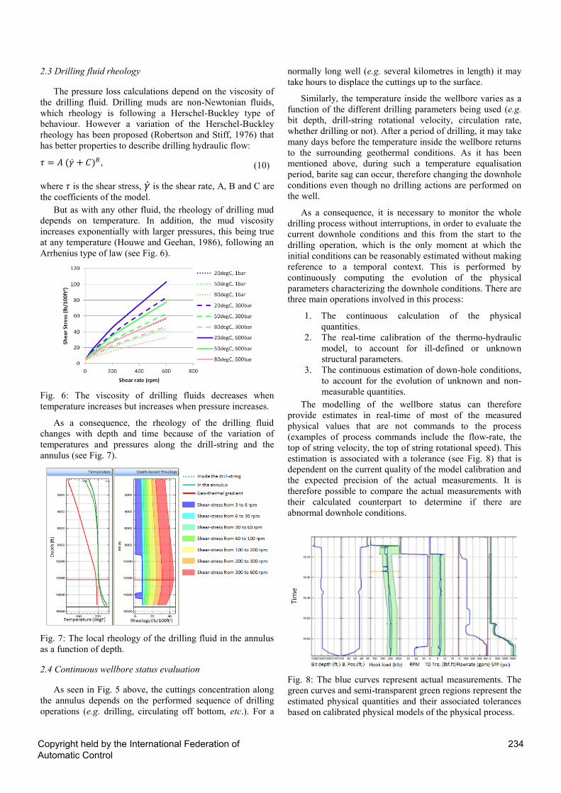
2.3 Drilling fluid rheology

The pressure loss calculations depend on the viscosity of

the drilling fluid. Drilling muds are non-Newtonian fluids,

which rheology is following a Herschel-Buckley type of

behaviour. However a variation of the Herschel-Buckley

rheology has been proposed (Robertson and Stiff, 1976) that

has better properties to describe drilling hydraulic flow:

( ̇ ) , (10)

where is the shear stress, ̇ is the shear rate, A, B and C are

the coefficients of the model.

But as with any other fluid, the rheology of drilling mud

depends on temperature. In addition, the mud viscosity

increases exponentially with larger pressures, this being true

at any temperature (Houwe and Geehan, 1986), following an

Arrhenius type of law (see Fig. 6).

Fig. 6: The viscosity of drilling fluids decreases when

temperature increases but increases when pressure increases.

As a consequence, the rheology of the drilling fluid

changes with depth and time because of the variation of

temperatures and pressures along the drill-string and the

annulus (see Fig. 7).

Fig. 7: The local rheology of the drilling fluid in the annulus

as a function of depth.

2.4 Continuous wellbore status evaluation

As seen in Fig. 5 above, the cuttings concentration along

the annulus depends on the performed sequence of drilling

operations (e.g. drilling, circulating off bottom, etc.). For a

normally long well (e.g. several kilometres in length) it may

take hours to displace the cuttings up to the surface.

Similarly, the temperature inside the wellbore varies as a

function of the different drilling parameters being used (e.g.

bit depth, drill-string rotational velocity, circulation rate,

whether drilling or not). After a period of drilling, it may take

many days before the temperature inside the wellbore returns

to the surrounding geothermal conditions. As it has been

mentioned above, during such a temperature equalisation

period, barite sag can occur, therefore changing the downhole

conditions even though no drilling actions are performed on

the well.

As a consequence, it is necessary to monitor the whole

drilling process without interruptions, in order to evaluate the

current downhole conditions and this from the start to the

drilling operation, which is the only moment at which the

initial conditions can be reasonably estimated without making

reference to a temporal context. This is performed by

continuously computing the evolution of the physical

parameters characterizing the downhole conditions. There are

three main operations involved in this process:

1. The continuous calculation of the physical

quantities.

2. The real-time calibration of the thermo-hydraulic

model, to account for ill-defined or unknown

structural parameters.

3. The continuous estimation of down-hole conditions,

to account for the evolution of unknown and non-

measurable quantities.

The modelling of the wellbore status can therefore

provide estimates in real-time of most of the measured

physical values that are not commands to the process

(examples of process commands include the flow-rate, the

top of string velocity, the top of string rotational speed). This

estimation is associated with a tolerance (see Fig. 8) that is

dependent on the current quality of the model calibration and

the expected precision of the actual measurements. It is

therefore possible to compare the actual measurements with

their calculated counterpart to determine if there are

abnormal downhole conditions.

Fig. 8: The blue curves represent actual measurements. The

green curves and semi-transparent green regions represent the

estimated physical quantities and their associated tolerances

based on calibrated physical models of the physical process.


234

An additional calibration difficulty occurs when there is a

long period of time without any measurements, such as when

it is necessary to pull out of hole (POOH) the drill-string to

perform the next drilling operation, or to replace a faulty

component in the BHA. In such cases, it is still possible to

perform the continuous calculation of the internal state of the

wellbore, but the error or uncertainty regarding the real

downhole conditions dramatically increases as it is no longer

possible to calibrate the physical models due to the lack of

real-time downhole measurements. Furthermore, heat transfer

in both natural convection and barite sag models are far from

accurate in those circumstances, thereby increasing the

uncertainty on the actual downhole conditions when the drill-

string is run back into the hole.

2.5 Mud pump start-up

The mud pump acceleration rates are ramped or stepped

up in such a manner that downhole pressures do not exceed

the fracturing pressure of the open hole formations. It is

important to estimate the effect of the downhole pressure

variations for the entire open hole well section and not only at

the casing shoe depth or at the bit depth, as is often done for

the sake of simplicity. In situations with complex or narrow

geo-pressure margins, the regions of maximum limitations

can be situated at various places along the open hole section.

The acceleration of the mud pumps must not set so as to

induce a downhole pressure pulse that exceeds the maximum

tolerable rock fracture limit. Such transient pressure surges

would not be visible using a steady state hydraulic model and

would result in allowing prohibitive mud pump accelerations

that could result in fracturing the formation. Our system

solves equations (1) and (2) using a finite difference method

that permit the estimation of acceleration effects on downhole

pressure along the open hole section of the well (see Fig. 9).

Fig. 9: Effect of ramping up the mud pumps on pump and

downhole pressures.

Ideally, to reduce pump start-up time, the flow rate should

be increased gradually and continuously to the target flow

rate. In practice, several stops need to be performed while

starting the mud pumps. Often, the driller desires to use

several intermediate steps to check that the pump pressure is

evolving normally. Each of these acceleration steps generate

a pressure build-up that stabilizes when steady state

conditions are reached. Therefore, independent pump

accelerations must be used for each single step, depending on

the current conditions and the following pump rate level.

It is therefore possible to calculate the maximum pump

acceleration from any given starting flow-rate to any other

target flow-rate while respecting the two conditions described

above: stay within the geo-pressure window and have a

monotonic increase of the pump pressure (see Fig. 10).

Using this 2 dimensional pump acceleration function, it is

possible to optimize the pump start-up procedure for any

number of stages in the ramping procedure.

Fig. 10: This graph shows the maximum acceptable pump

acceleration while starting from a given flow-rate to reach a

target flow-rate.

2.6 Maximum pump rate

Based on the maximum downhole pressure limit (for

example using the fracturing pressure prognosis), it is

possible to calculate an absolute maximum flow rate that

guarantees that the downhole pressure will remain below the

upper pressure boundary. To calculate that flow-rate limit,

only steady state conditions are necessary (no need to account

for mud pump accelerations) and therefore a simpler version

of the hydraulic model can be used. The partial derivative on

time of equation (2) can be considered to be 0 and the axial

velocity of drill-string is supposed to be constant. The

resulting simplified equation can easily be solved by

integrating along the curvilinear abscissa for each branch of

the hydraulic circuit:

( ) ∫ ( ) ( ( ))

( )

(11)

where p is the pressure that should be calculated, is the

measured depth at which the pressure shall be calculated,

is the initial measured depth of the branch, is the

initial pressure at , ( ) is the inclination at the

curvilinear abscissa s,

is the frictional pressure loss

gradient.

This maximum flow rate changes with time, bit depth and

other operational parameters like the rotational velocity or the

axial velocity of the string. The dependency on time is due to

downhole temperature variations. Another dependency is

depth. The position of larger BHA elements with regard to

different formation layers influences the maximum tolerable

flow rate. The rotational velocity of the drill-string is also


235

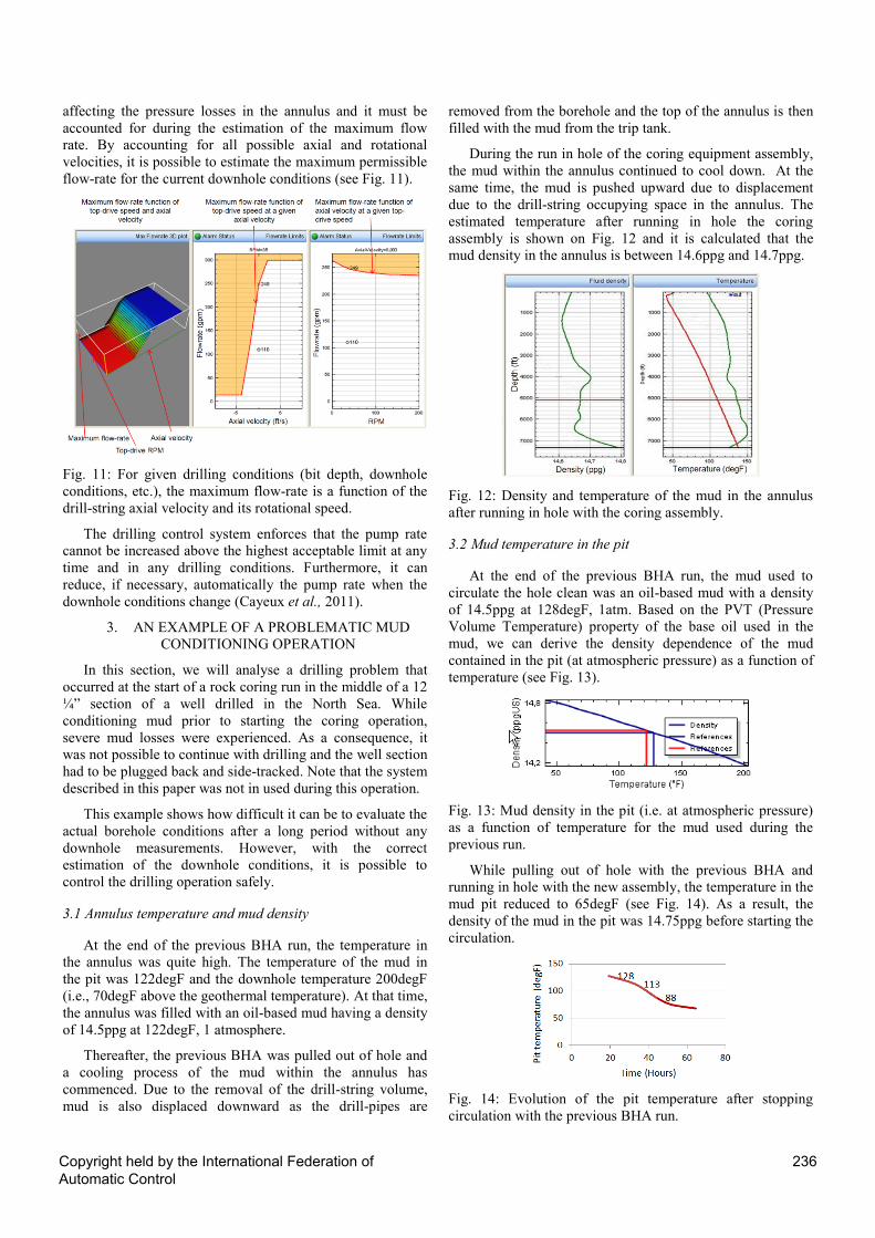
affecting the pressure losses in the annulus and it must be

accounted for during the estimation of the maximum flow

rate. By accounting for all possible axial and rotational

velocities, it is possible to estimate the maximum permissible

flow-rate for the current downhole conditions (see Fig. 11).

Fig. 11: For given drilling conditions (bit depth, downhole

conditions, etc.), the maximum flow-rate is a function of the

drill-string axial velocity and its rotational speed.

The drilling control system enforces that the pump rate

cannot be increased above the highest acceptable limit at any

time and in any drilling conditions. Furthermore, it can

reduce, if necessary, automatically the pump rate when the

downhole conditions change (Cayeux et al., 2011).

3. AN EXAMPLE OF A PROBLEMATIC MUD

CONDITIONING OPERATION

In this section, we will analyse a drilling problem that

occurred at the start of a rock coring run in the middle of a 12

¼” section of a well drilled in the North Sea. While

conditioning mud prior to starting the coring operation,

severe mud losses were experienced. As a consequence, it

was not possible to continue with drilling and the well section

had to be plugged back and side-tracked. Note that the system

described in this paper was not in used during this operation.

This example shows how difficult it can be to evaluate the

actual borehole conditions after a long period without any

downhole measurements. However, with the correct

estimation of the downhole conditions, it is possible to

control the drilling operation safely.

3.1 Annulus temperature and mud density

At the end of the previous BHA run, the temperature in

the annulus was quite high. The temperature of the mud in

the pit was 122degF and the downhole temperature 200degF

(i.e., 70degF above the geothermal temperature). At that time,

the annulus was filled with an oil-based mud having a density

of 14.5ppg at 122degF, 1 atmosphere.

Thereafter, the previous BHA was pulled out of hole and

a cooling process of the mud within the annulus has

commenced. Due to the removal of the drill-string volume,

mud is also displaced downward as the drill-pipes are

removed from the borehole and the top of the annulus is then

filled with the mud from the trip tank.

During the run in hole of the coring equipment assembly,

the mud within the annulus continued to cool down. At the

same time, the mud is pushed upward due to displacement

due to the drill-string occupying space in the annulus. The

estimated temperature after running in hole the coring

assembly is shown on Fig. 12 and it is calculated that the

mud density in the annulus is between 14.6ppg and 14.7ppg.

Fig. 12: Density and temperature of the mud in the annulus

after running in hole with the coring assembly.

3.2 Mud temperature in the pit

At the end of the previous BHA run, the mud used to

circulate the hole clean was an oil-based mud with a density

of 14.5ppg at 128degF, 1atm. Based on the PVT (Pressure

Volume Temperature) property of the base oil used in the

mud, we can derive the density dependence of the mud

contained in the pit (at atmospheric pressure) as a function of

temperature (see Fig. 13).

Fig. 13: Mud density in the pit (i.e. at atmospheric pressure)

as a function of temperature for the mud used during the

previous run.

While pulling out of hole with the previous BHA and

running in hole with the new assembly, the temperature in the

mud pit reduced to 65degF (see Fig. 14). As a result, the

density of the mud in the pit was 14.75ppg before starting the

circulation.

Fig. 14: Evolution of the pit temperature after stopping

circulation with the previous BHA run.


236

The density difference between the mud being pumped

from the mud pit and the downhole drilling fluid is confirmed

by a gravity induced mud displacement while filling the drill-

string before starting the mud conditioning operation. It is

observed burst of flow in the return channel much earlier than

any pump pressure could indicate that the drill-string was

filled. Furthermore the volume of fluid being pumped to fill

the drill-string was much larger than anticipated (see Fig. 15).

Fig. 15: After filling the pipes for 7 minutes, mud returns

could be observed in the return channel.

3.3 Circulation

At the start of the circulation process, the observed and

calculated SPP (Stand Pipe Pressure) almost perfectly

matched. However, after a further 13 minutes of circulation, a

deviation between the observed and calculated SPP could be

noticed (see Fig. 16).

Fig. 16: Deviation between measured and calculated SPP.

This deviation amplified itself and then stabilized to a

maximum of 70psi (i.e., 5 bars). If the abnormally high SPP

was due to an increase of the pressure within the annulus,

then the downhole pressure could be very close to the

fracturing pressure gradient.

We notice that both the calculated and observed SPP

increase during the circulation process. This is because the

calculated pressure accounts for the heat transfer and the

estimated local mud density being transported out of the hole.

But the temperature effect is not enough to explain the

discrepancy between the modelled values and the actual SPP

measurements.

However, we can also notice that the deviation between

the calculated and observed SPP begin a few minutes after

lowering the drill-string to the bottom of the hole. A

supposition could be that the last 100ft were filled with a very

heavy mud due to barite sag.

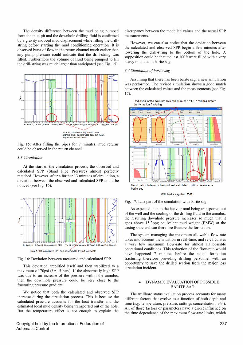
3.4 Simulation of barite sag

Assuming that there has been barite sag, a new simulation

was performed. The revised simulation shows a good match

between the calculated values and the measurements (see Fig.

17).

Fig. 17: Last part of the simulation with barite sag.

As expected, due to the heavier mud being transported out

of the well and the cooling of the drilling fluid in the annulus,

the resulting downhole pressure increases so much that it

goes above 15.3ppg equivalent mud weight (EMW) at the

casing shoe and can therefore fracture the formation.

The system managing the maximum allowable flow-rate

takes into account the situation in real-time, and re-calculates

a very low maximum flow-rate for almost all possible

operational conditions. This reduction of the flow-rate would

have happened 7 minutes before the actual formation

fracturing therefore providing drilling personnel with an

opportunity to save the drilled section from the major loss

circulation incident.

4. DYNAMIC EVALUATION OF POSSIBLE

BARITE SAG

The wellbore status evaluation process accounts for many

different factors that evolve as a function of both depth and

time (e.g. temperature, pressure, cuttings concentration, etc.).

All of those factors or parameters have a direct influence on

the time dependence of the maximum flow-rate limits, which


237

is in itself a function of drilling parameters (i.e., the axial and

rotational velocity of the drill-string). However, as shown in

the above example, barite sag can have a major influence on

the acceptable maximum flow-rate to be used during mud

conditioning. Unfortunately, it is difficult to have a barite sag

model that is accurate enough to reflect the real downhole

conditions simply because the barite sag properties of the

mud are not measured during drilling operations.

An alternative solution is to assume that there has been

barite sag in the well and to then fit the side effects of such an

uneven concentration of weighting materials along the

annulus with the observed evolution of the downhole

pressure (if it is available) and the pump pressure. An

Unscented Kalman filter technique is very well suited for

such a dynamic fitting (Gravdal et al., 2010). Using the

current best estimate of the mud density concentration prior

to the start of circulation, it is possible to adjust the actual

limits of the flow-rate to lift up the dense, concentrated mud

during a drilling fluid conditioning operation and therefore

improve the desired safe operating window for the mud

pumps.

5. CONCLUSIONS

This paper has described the complexity in safely

managing mud pump operations to avoid formation

fracturing. The pump operating limits to be applied are

context dependent both in terms of operational parameters

but also as a function of the downhole conditions. It is

especially challenging to obtain a safe flow-rate management

when conditioning mud because the temperature evolution

can drastically change within a short period of time. It is even

more complicated to account for potential barite sag

conditions because little information is available before the

circulation is effectively started, but dynamic calibration of

plausible concentrations of high gravity solids along the

annulus can help determine the maximum flow-rate

acceptable to condition the mud.

REFERENCES

Aas B., Merlo A., Rommetveit R, Sterri N. (2005). A Method

to Characterise the Propensity for Dynamic Sagging of

Weight Materials in Drilling Fluids. Annual Transactions

of the Nordic Rheology Society, Volume 13, pp. 91-98.

Cayeux E., B. Daireaux, E. W. Dvergsnes (2011).

Automation of Mud-Pump Management : Application to

Drilling Operations in the North Sea. SPE Drilling &

Completion, March 2011, Volume 26 (1), pp. 41-51.

Corre B., Eymard R., Guenot A. (1984). Numerical

Computation of Temperature Distribution in a Wellbore

While Drilling. SPE Annual Technical Conference and

Exhibition, Houston, Texas, USA, 16-19 September 1984.

Dye W., Hemphill T., Gusler W., Mullen G. (2001).

Correlation of Ultralow-Shear-Rate Viscosity and

Dynamic Barite Sag. SPE Drilling & Completion, March

2001, Volume 16 (1), pp. 27-34.

Ekwere J.P., Chenevert M., Chunhai Zhang, (1990). A Model

for Predicting the Density of Oil-Based Muds at High

Pressures and Temperatures. SPE Drilling Engineering,

June 1990, Volume 5 (2), pp. 141-148.

Fjelde K.K., Rommetveit R., Merlo A., Lage A. (2003).

Improvements in Dynamic Modeling of Underbalanced

Drilling. SPE/IADC Underbalanced Technology

Conference and Exhibition, Houston, Texas, USA, March

25-26, 2003.

Gravdal J.E., Lorentzen R.J., Fjelde K.K., Vefring E. (2010).

Tuning of Computer Model Parameters in Managed-

Pressure Drilling Applications Using an Unscented-

Kalman-Filter Technique. SPE Journal, September 2010,

Volume 15(3), pp. 856-866.

Howe O.H., Geehan T. (1986). Rheology of Oil-Based Muds.

SPE Annual Technical Conference, New Orleans,

Lousiana, USA, Octobrer 5-8, 1986.

Iversen F., Cayeux E., Dvergsnes E.W., Ervik R., Welmer M.

and Balov M.K. (2009). Offshore Field Test of a New

System for Model Integrated Closed Loop Drilling

Control. SPE Drilling & Completion, December 2009,

Volume 24 (4), pp. 518-530.

Kuru E., Okunsebor O.M., Li Y. (2005). Hydraulic

Optimization of Foam Drilling For Maximum Drilling

Rate in Vertical Wells. SPE Drilling & Completion,

December 2005, Volume 20 (4), pp. 258-267.

Larsen T.I., Pilehvari A.A., Azar J.J. (1997). Development of

a New Cuttings-Transport Model for High-Angle

Wellbores including Horizontal Wells. SPE Drilling &

Completion, June 1997, Volume 12 (2), pp. 129-136,

SPE-25872

Marshall D.W., Bentsen R.G. (1982). A Computer Model to

Determine the Temperature Distributions in a Wellbore.

The Journal of Canadian Petroleum Technology, Jan.-

Feb. 1982, Volume 21 (1), pp.63-75

Monteiro E.N., Ribeiro P.R., Lomba R.F.T. (2010). Study of

the PVT Properties of Gas-Synthetic-Drilling-Fluid

Mixtures Applied to Well Control. SPE Drilling &

Completion, March 2010, Volume 25 (1), pp. 45-52.

Robertson R.E., Stiff H.A. (1976). An Improved

Mathematical Model for Relating Shear Stress to Shear

Rate in Drilling Fluids. SPE Journal, February 1976,

Volume 16 (1), pp. 31-36.

Scott P. (2009). Real-Time Monitoring of Down Hole ECDs

for Parasite Aeration Using a Simple Spreadsheet

Calculation. IADC/SPE Managed Pressure Drilling and

Underbalanced Operations Conference and Exhibition,

San Antonio, Texas, USA, 12-13 February 2009.


238

Documents

Safe Mud Pump Management While Conditioning … a methodology that is used in an automatic drilling control system ... (especially with oil -based mud) ... Safe Mud Pump Management