S⃝e MR - semr.math.nsc.rusemr.math.nsc.ru/v12/p884-900.pdf · MESOSCOPIC DYNAMICS OF SOLID-LIQUID INTERFACES. A GENERAL MATHEMATICAL MODEL A. MEIRMANOV, N. OMAROV, V. TCHEVERDA,

S e⃝MR ISSN 1813-3304

СИБИРСКИЕ ЭЛЕКТРОННЫЕМАТЕМАТИЧЕСКИЕ ИЗВЕСТИЯ

Siberian Electronic Mathematical Reportshttp://semr.math.nsc.ru

Том 12, стр. 884–900 (2015) УДК 532.65DOI 10.17377/semi.2015.12.075 MSC 76D45

MESOSCOPIC DYNAMICS OF SOLID-LIQUID INTERFACES.A GENERAL MATHEMATICAL MODEL

A. MEIRMANOV, N. OMAROV, V. TCHEVERDA, A. ZHUMALY

Abstract. A number of chemical and physical processes occur atinterfaces where solids meet liquids. Among them is heap and in-situleaching, an important technological process to extract uranium, preciousmetals, nickel, copper and other compound. To understand the mainpeculiarities of these processes a general mathematical approach is deve-loped and applied. Its key point is new conditions at the free (unknown)boundary between liquid and solid phases (pore space-solid skeleton).The developed model can be used to analyze the dependence of thedynamics of the free fluid-skeleton interface on the external parametersof the process, like temperature, pressure, reagent concentration andothers. Therefore, the overall behavior of the process can be controlledeither by the rate of chemical reaction on the free interface via reagentconcentration or by the velocity at which dissolved substances are trans-ported to or from the free surface.

The special attention is paid to a plausible justification of upscalingfrom mesoscopic to macroscopic scales and its comparison with approa-ches usually used at the moment. Several examples illustrate the feasibi-lity of the models.

Keywords: solid-liquid interface, leaching, fluid flow.

1. Introduction

Ability to control chemical and physical processes at interfaces is important tocontrol a variety of technological processes, in particular heap and in-situ leaching.

Meirmanov, A., Omarov, N., Tcheverda, V., Zhumaly, A., Mesoscopic Dynamics ofSolid-Liquid Interfaces. A General Mathematical Model.

c⃝ 2015 Meirmanov A., Omarov N., Tcheverda V., Zhumaly A.The work is supported by grants of the Ministry of Education and Science of Kazakhstan

Republic, 0980/GF4 and 0981/GF4.Received October, 18, 2015, published December, 3, 2015.

884

MESOSCOPIC DYNAMICS OF SOLID-LIQUID INTERFACES 885

For this purpose it should be possible to perform numerical simulation and analysisof the processes under consideration. So far these processes are described at themacroscopic scale by the variety of mathematical models (see [1], [2], [3], [4], andreferences there in). As a rule, people deal with so called phenomenological twophase models when at each point of a continuous medium there are both the solidskeleton and the liquid. All these models are based on the same principles:

• Fluid dynamics is described by Darcy’s system of filtration or some itsmodification;

• The migration of active compound and products of chemical reactions aredescribed by somehow postulated convection-diffusion equations for theappropriate concentrations.

The main thing in these postulates is the form and coefficients of differentialequations. There is a variety of approaches how to choose in dependence of thetastes and preferences of the authors. It is quite explainable because the basicmechanism of the physical process on the macroscale is formed on microscale of theunknown (free) boundary between the pore space and the solid skeleton. But exactlythis basic mechanism is not used in the models! Really, dissolution of rocks takesplace exactly there, the concentration of the injected reagent and the geometry ofthe pores are changed on this interface as well. Moreover, the flow of the products ofchemical reactions inward the pore space is generated on this scale also. But at thesame time, all of the aforementioned standard macroscopic mathematical modelsoperate with other, much larger, scales and hence just do not "see" neither freeboundary nor peculiarities of the interaction of the reagent and skeleton on thisboundary. This explains such a variety of macroscopic mathematical models.

R. Burridge and J. B. Keller [5] and E. Sanchez-Palencia [6] were the first whoexplicitly stated that mathematical models to describe multiscale processes mustbe rigorously derived from micro- to macroscale by the following successive steps:

(a) to develop a mathematical model describing the physical process at themicroscopic level with maximal accuracy (exact model);

(b) to distinguish a set of small parameters characterizing difference in scales ofthe model;

(c) to derive the macroscopic model as the asymptotic limit of the exact model.Various particular implementations of this approach are analysed in [7], [8].

The most systematic implementation of this scheme have been studied by A. Meir-manov [8] – [12] on the base of dimensionless forms of the mathematical models. Inthis way it becomes possible to simplify microscopic mathematical models and tofind exact asymptotic approximations, adequately describing physical processes atthe macroscopic level.

In what follows we implement the stages (a)-(c) on the theoretical level. To dothat we use the above mentioned Meirmanov’s approaches and models [8] togetherwith methods, developed for the free boundary problems [13].

The paper deals with a dissolution of a solid porous skeleton by an activeadmixture (acid) dissolved in an inviscid incompressible pore liquid. As a resultof a dissolution of the solid skeleton appear products of chemical reactions. Theprocess is considered in a bounded domain Ω ⊂ R3 with boundary S. Next, let usconsider S+ ⊂ S as a set of injection wells, S− ⊂ S is considered as productionwells, while S0 ⊂ S represents impermeable insoluble piece of the boundary.

886 A. MEIRMANOV, N. OMAROV, V. TCHEVERDA, A. ZHUMALY

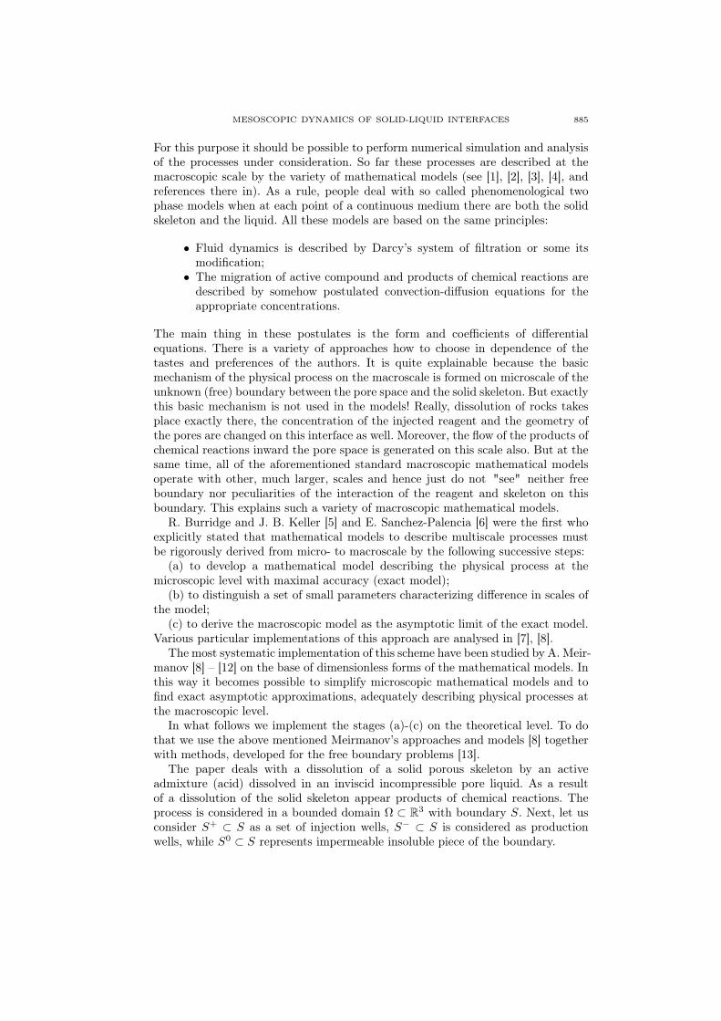
Fig. 1. The pore space.

In order to introduce the microscale level of the process, the domain Ω is treatedas consisting of the pore space Ωf (t), and the solid skeleton Ωs(t). The dissolutionprocess takes place at the interface Γ(t) between the pore space and solid skeleton(see Fig. 1). It is worth mentioning that Γ(t) is a free (unknown) surface, becauseduring the leaching the skeleton is dissolved and changes its shape. These mathe-matical problems are called free boundary problems.

The mathematical model of leaching at the microscale is based on classicalequations of continuum mechanics and some trustworthy relations characterizingwell-known chemical reactions [14]. To complete the model we need to derivea new boundary conditions, describing dissolution of the solid skeleton at thefree boundary and dynamics of the boundary itself. The next step is the properdescription of the process at the macroscale, known as upscaling or homogenization.To perform this step correctly we need very new developments in mathematicsdealing with "two-scale convergence"([8],[9]).

Let us begin with some general remarks to describe the steps doing to derivethe mathematical model of the leaching at the microscale. For the first of all, fluidflow in pores at the microscopic level is very slow (a few meters per year) thereforethe convection terms in Navier-Stokes equations can be neglected, hence Stokesequations for incompressible viscous liquids are good approximation. The correctmathematical model of propagation of active admixtures in pore space (microscopiclevel) should take into account the both convection and diffusion. Really, withoutdiffusion the reverse flow of the reaction products from the free surface Γ(t) inwardthe pore space blocks the flow of the reagent and finally cancels chemical reaction.Thus, the diffusion – convection equation must be used to describe propagation ofthe active reagent (acid).


For the concentrations of the products of chemical reactions we use the transportequations without diffusion terms. This equation is of the first order in space andneeds boundary condition only on the parts of the boundary ∂Ωf (t) where theliquid starts the motion inward the pore space, that is at the free boundary Γ(t)and injection wells S+

i .Looking ahead let us note, that a diffusion process in the liquid is also very

slow, therefore to balance the process some oscillations should happen, at leastat the initial stage. Really, the rate of outflow of fluid from the free boundary isproportional to the concentration of the acid and grows when this concentrationincreases. The domination of outflow of fluid from the free boundary makes lessthe diffusion of the reagent and leads to decreasing of its concentration at the freeboundary. In turn, it implies the decreasing of the outflow of fluid from the freeboundary and the domination of the diffusion of the acid to the free boundary. Thegrowth of the diffusion of the reagent to the free boundary leads to the growth ofits concentration at the free boundary and so on.

2. Mathematical model of the leaching for microscopic model

2.1. Statement of the initial-boundary value problem for the microscopiclevel. Let us introduce characteristic length L and time T . In dimensionless variables

x → x

L, t → t

T, v → T

Lv, p → p∗ p,

the dynamics of liquid in pore space Ωf (t) is described by Stokes equation

(1) αµ v −∇ p = 0,

for the pressure p and velocity v.The continuity equation is used in its generalized form [15], that is as a continuity

equation for a generalized motion of continuum media including solid skeleton,where v ≡ 01:

(2)∂ϱ

∂t+∇ · (ϱv) = 0.

Equation (2) is treated in the sense of distributions, that is as an integral identity∫ΩT

ϱ

(∂φ

∂t+ v · ∇φ

)dxdt = 0

for the densityϱ(x, t) = χ(x, t)ϱf +

(1− χ(x, t)

)ϱs,

which holds for any smooth probe function φ(x, t), vanishing at S+, S−, t = 0 andt = T .

In particular it follows the boundary condition [15]:

(vn − Vn)ϱf = −Vnϱs, x ∈ Γ(t), t > 0,

or

(3) vn = −Vn(ϱs − ϱf )

ϱf⇐⇒ Vn − vn =

ϱsϱf

Vn, x ∈ Γ(t), t > 0,

1The skeleton is immobile!


where Vn is the velocity of the free boundary S and vn is the normal velocity ofthe fluid at this boundary. Finally, the continuity equation in its differential formin the pore space Ωf (t) for t > 0 is written as

(4) ∇ · v = 0.

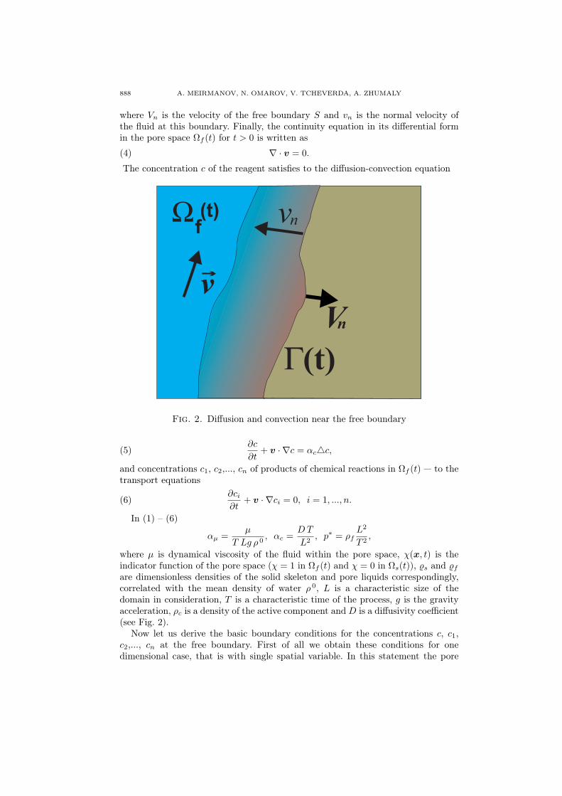
The concentration c of the reagent satisfies to the diffusion-convection equation

Fig. 2. Diffusion and convection near the free boundary

(5)∂c

∂t+ v · ∇c = αcc,

and concentrations c1, c2,..., cn of products of chemical reactions in Ωf (t) — to thetransport equations

(6)∂ci∂t

+ v · ∇ci = 0, i = 1, ..., n.

In (1) – (6)

αµ =µ

T Lg ρ 0, αc =

DT

L2, p∗ = ρf

L2

T 2,

where µ is dynamical viscosity of the fluid within the pore space, χ(x, t) is theindicator function of the pore space (χ = 1 in Ωf (t) and χ = 0 in Ωs(t)), ϱs and ϱfare dimensionless densities of the solid skeleton and pore liquids correspondingly,correlated with the mean density of water ρ 0, L is a characteristic size of thedomain in consideration, T is a characteristic time of the process, g is the gravityacceleration, ρc is a density of the active component and D is a diffusivity coefficient(see Fig. 2).

Now let us derive the basic boundary conditions for the concentrations c, c1,c2,..., cn at the free boundary. First of all we obtain these conditions for onedimensional case, that is with single spatial variable. In this statement the pore


space is considered as Ωf (t) = x : 0 < x < X(t) and Γ(t) = x : x = X(t) be afree boundary (see Fig. 3). Then

(7)

∂v

∂x= 0, 0 < x < X(t),

∂c

∂t+ v

∂c

∂x= αc

∂2c

∂x2, 0 < x < X(t),

αc∂c

∂x− v(t) c = 0 at x = 0,

∂ci∂t

+ v∂ci∂x

= 0, 0 < x < X(t), ci = 0 at x = 0, i = 1, ..., n.

The total masses of the reagent and products of the reactions in Ωf (t) are given bythe integrals

(8) M(t) =

∫ X(t)

0

c(x, t)dx, Mi(t) =

∫ X(t)

0

ci(x, t)dx, i = 1, ..., n.

The rate of change of these variables in time is computed as:

dM

dt=

dX

dtc(X(t), t

)+

∫ X(t)

0

=∂c

∂t(x, t)dx

=dX

dtc(X(t), t

)+

∫ X(t)

0

∂

∂x

(αc

∂c

∂x(x, t)− v(t) c(x, t)

)dx

=

(dX

dt(t)− v(t)

)c(X(t), t) + αc

∂c

∂x(X(t), t),

dMi

dt=

dX

dtci(X(t), t

)+

∫ X(t)

0

∂ci∂t

(x, t)dx

=dX

dtci(X(t), t

)−

∫ X(t)

0

v(t)∂ci∂x

(x, t)dx

=

(dX

dt(t)− v(t)

)ci(X(t), t) =

ϱsϱf

dX

dtci(X(t), t), i = 1, ..., n.

Straightforward calculations of these integrals with the use of (3) and (7) at x = 0,gives:

(9)

dM

dt= (

dX

dt− v)c+ αc

∂c

∂x,

dMi

dt=

ϱsϱf

dX

dtci, i = 1, ..., n, at x = X(t).

Last relations mean that the change of concentrations of products of chemical

reactions occurs only at Γ(t). The valuesdM

dt,dMi

dt, i = 1, . . . , n, are called rates


of chemical reactions and are defined from the complimentary laws of chemicalkinetics:

(10)dM

dt= −β φ(c),

dMi

dt= β φi(c), i = 1, ..., n,

where φ(c), φi(c), i = 1, ..., n are given positive functions.On the other hand, the mass conservation implies

(11) ϱsdX

dt− ϱf

dM

dt=

n∑i=1

ϱidMi

dt,

where ϱc, ϱ1, ..., ϱn are dimensionless densities of reagent and products of chemicalreactions.

Relations (9)–(11) result

(12)dX

dt(t) = β φ0 (c (X(t), t)) , ci(X(t), t) = φi

(c(X(t), t

)), i = 1, ..., n,

and

(13)(dXdt

(t)− v(t))c(X(t), t) + αc

∂c

∂x(X(t), t) = −β φ

(c(X(t), t

)),

where

ϱsφ0 + ϱcφ =n∑

i=1

ϱiφi, φi =ϱsϱf

φi

φ0, i = 1, . . . , n.

Coming back to (4) – (6) we conclude that in a general case mass conservation lawsfor concentrations at the free boundary have a form

(14) (Vn − vn) c+ β φ(c) + αc∂c

∂n= 0, x ∈ Γ(t),

(15) ci = φi(c), i = 1, . . . , n, x ∈ Γ(t),

(16) Vn = β φ0(c), x ∈ Γ(t),

where Vn is a normal velocity of Γ(t) in the direction of the outward to Ωf (t) normal

n, vn = v ·n is a normal liquid velocity, and∂c

∂n= ∇c ·n is a normal derivative of

c at Γ(t).It remains to supplement differential equations by missing boundary and initial

conditions.At the free boundary Γ(t) the tangent velocity of the pore liquid vanishes:

(17) v − v · n = 0.

At the boundaries S+ and S−, which give injection and production wells, we putthe normal tension in the liquid

(18)(αµ D(v)− p I

)· n = −p±(x, t)n,

where I is the unit matrix and

D(v) =1

2(∇v +∇v∗).

At the injection wells S+ we put concentrations of the reagent and products ofchemical reactions

(19) ci = 0, i = 1, . . . , n, c = c+(x, t).


At the production wells

(20) ∇c · n = 0.

On the impermeable boundary S0

(21) v = 0, ∇c · n = 0.

The problem is ended with initial conditions

(22) Γ(0) = Γ0, c(x, 0) = c0(x), ci(x, 0) = 0, i = 1, ..., n, x ∈ Ω0.

The system of differential equations (1), (4), (5), (6), completed with boundaryand initial conditions (3), (14) – (22) forms desired mathematical model describingleaching at the microscopic level.

Note that the problem (1), (3)-(5), (14), (16)–(18), (20)-(22) for the liquidvelocity and pressure, concentration of the active admixture, and the free boundaryis independent of the problem (6), (15), (19), (22) for concentrations of products ofchemical reactions.

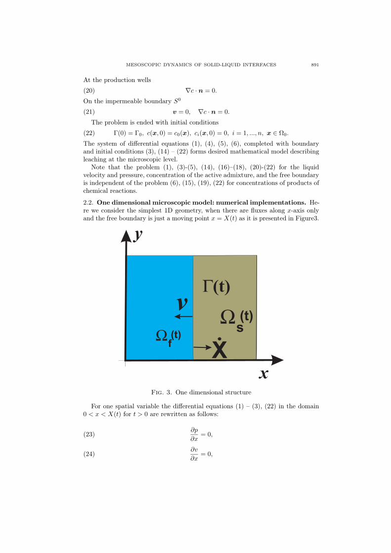
2.2. One dimensional microscopic model: numerical implementations. He-re we consider the simplest 1D geometry, when there are fluxes along x-axis onlyand the free boundary is just a moving point x = X(t) as it is presented in Figure3.

Fig. 3. One dimensional structure

For one spatial variable the differential equations (1) – (3), (22) in the domain0 < x < X(t) for t > 0 are rewritten as follows:

(23)∂p

∂x= 0,

(24)∂v

∂x= 0,


(25)∂c

∂t+ v

∂c

∂x= αc

∂2c

∂x2,

(26)∂ci∂t

+ v∂ci∂x

= 0, i = 1, ..., n.

Boundary and initial conditions (14) – (22) are transformed to

(27) p(0, t) = p+(t), c (0, t) = c+(t), t > 0,

(28)dX

dt= β φ0(c), x = X(t), t > 0,

(29)(dXdt

− v)c+ β φ(c) + αc

∂c

∂x= 0, x = X(t), t > 0,

(30) ci(X(t), t) = φi(c), i = 1, ..., n, x = X(t), t > 0,

(31) v (t) = −dX

dt(t)

(ρs − ρf )

ρf, t > 0,

(32) X(0) = X0, c(x, 0) = c0(x), 0 < x < X0.

Let us consider some particular behavior of chemical reaction:

(33) φ(c) = c ν , φi(c) = βi cν 0

where ν1 = ν − ν0 > 0. It follows

(34) φ0(c) = δ0cν0(1− δ1 c

ν 1), φi(c) =γi

(1− δ1 c ν 1),

where

δ0 =n∑

i=1

ϱiϱs

βi, δ1 =ϱc

ϱs δ0< 1.

Let us fix now the characteristic length L = 40 µm, time T = 1 sec, δ0 = 1,δ1 = 0, 5, γ1 = 0, 01, ν1 = 0, 2 and suppose that the product of the chemicalreaction is the single substance, that is n = 1. Now let us analyze how does theconcentration of the product of chemical reaction at free boundary changes fordifferent β, ν0 and c+.

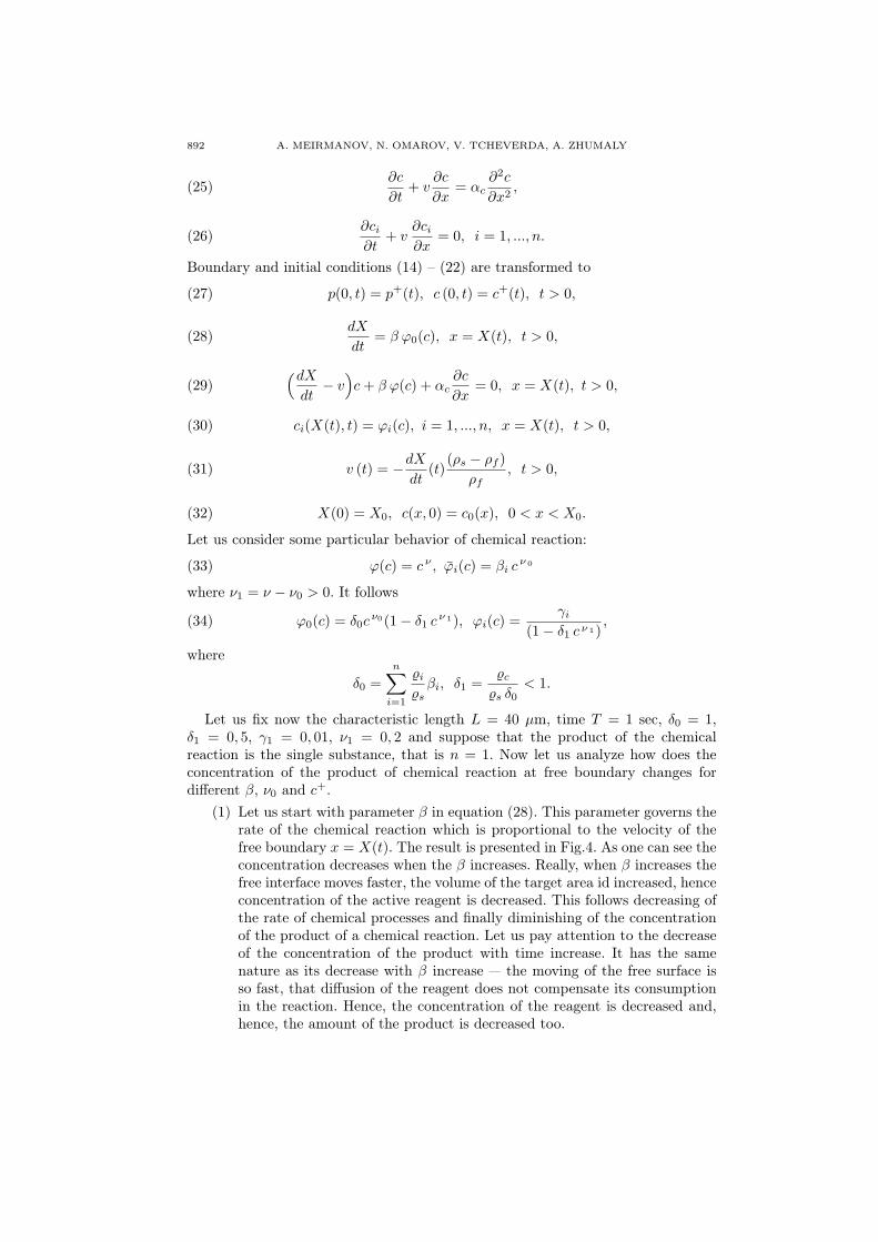
(1) Let us start with parameter β in equation (28). This parameter governs therate of the chemical reaction which is proportional to the velocity of thefree boundary x = X(t). The result is presented in Fig.4. As one can see theconcentration decreases when the β increases. Really, when β increases thefree interface moves faster, the volume of the target area id increased, henceconcentration of the active reagent is decreased. This follows decreasing ofthe rate of chemical processes and finally diminishing of the concentrationof the product of a chemical reaction. Let us pay attention to the decreaseof the concentration of the product with time increase. It has the samenature as its decrease with β increase — the moving of the free surface isso fast, that diffusion of the reagent does not compensate its consumptionin the reaction. Hence, the concentration of the reagent is decreased and,hence, the amount of the product is decreased too.


Fig. 4. Concentration of product of chemical reaction at the freeboundary for different β

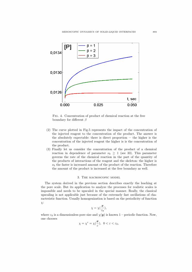
(2) The curve plotted in Fig.5 represents the impact of the concentration ofthe injected reagent to the concentration of the product. The answer isthe absolutely expectable: there is direct proportion — the higher is theconcentration of the injected reagent the higher is is the concentration ofthe product.

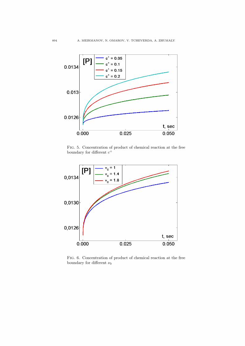
(3) Finally let us consider the concentration of the product of a chemicalreaction in dependence of parameter ν0 ≥ 1 (see 33). This parametergoverns the rate of the chemical reaction in the part of the quantity ofthe products of interactions of the reagent and the skeleton: the higher isν0 the faster is increased amount of the product of the reaction. Thereforethe amount of the product is increased at the free boundary as well.

3. The macroscopic model

The system derived in the previous section describes exactly the leaching atthe pore scale. But its application to analyze the processes for realistic scales isimpossible and needs to be upscaled in the special manner. Really, the classicalupscaling is not applicable just because of the extremely fast oscillations of cha-racteristic function. Usually homogenization is based on the periodicity of functionχ:

χ = χ(x

ε0),

where ε0 is a dimensionless pore size and χ(y) is known 1 – periodic function. Now,one chooses

χ = χε = χ(x

ε), 0 < ε < ε0,


Fig. 5. Concentration of product of chemical reaction at the freeboundary for different c+

Fig. 6. Concentration of product of chemical reaction at the freeboundary for different ν0


and let ε goes to zero. The homogenization consists of finding the limit of corres-ponding to χε solutions vε, pε, cε, cεi and the homogenized system for these limits.For sufficiently small ε0 the solution to this homogenized system is closed to thesolution for χ = χε0 .

For our case the characteristic function of the pore space χ is variable in timeand space and is given at t = 0 only. To solve the problem we suppose that

χ = χε = χ(x, t,x

ε) + o(ε), 0 < ε < ε0,

where χ(x, t,y) is 1-periodic in y function, and construct the upscaled systemof equations as ε → 0. Mathematically implementation of this approach is toocomplicated due to nonlinearity of the problem and necessity to search for unknowncharacteristic function χε. Therefore at the moment we choose to be restricted withformal, but still physically justified, easier version of upscaling (homogenization)which is based on the representations:

β = λ ε, αµ = µ1ε2, αc = D0,

vε(x, t) = V (x, t,x

ε) + o(ε),

pε(x, t) = p(x, t) + o(ε),

cε(x, t) = c(x, t) + o(ε), ∇ cε(x, t) = ∇ c(x, t) +∇yC(x, t,x

ε) + o(ε),

cεi (x, t) = ci(x, t) + o(ε), i = 1, . . . , n

with 1-periodic in y functions V (x, t,y) and C(x, t,y).Using these representations and well – known mathematical formula

limε→0

∫Q

U(x, t,x

ε)dx =

∫Q

(∫Y

U(x, t,y)dy)dx

for 1-periodic in y ∈ Y function U(x, t,y), we find homogenized system for functions

v(x, t) =

∫Y

V (x, t,y)dy, p(x, t), and c(x, t) with unknown coefficients.

More precisely, this system consists of dynamic equations

(35) v = − 1

µ1A · ∇p,

(36) ∇ · v =(ϱs − ϱf )

ϱf

∂ m

∂t

for the velocity v and pressure p of pore liquid, and the diffusion – convectionequation

(37) m∂ Φ(c)

∂t+ v · ∇ c−D0 ∇ ·

(C · ∇c) = −

( ϱsϱf

c+φ(c)

φ0(c)

) ∂ m

∂t

for concentration c of the reagent. Here Φ(c) = c +φ(c)

φ0(c)and unknown functions

m (porosity of a medium) is given as:

m(x, t) =

∫Y

χ(x, t,y)dy.


Matrices A and C are defined by a given microstructure. In particular:

C(x, t) =(m(x, t) I+

∫Y

χ(x, t,y)( 3∑i=1

∇yQ(i)(x, t,y)⊗ ei

)dy

),

with unit matrix I and the standard cartesian basis (e1, e2, e3). The product B =a⊗ b is defined as B · c = a(b · c). The 1 – periodic in y functions Q(i)(x, t,y), i =1, 2, 3 in each point x ∈ Ω for t > 0 are solutions to the following periodic boundaryproblem

(38) yQ(i) = 0, y ∈ Yf (x, t),

(39) (ei +∇yQ(i)) · ν = 0, y ∈ γ(x, t) = ∂ Yf (x, t)

in the unknown subdomain Yf (x, t) ⊂ Y of the unit cube Y . In (39) ν is the unitnormal vector to the boundary γ(x, t).

By analogy with the microscopic model, the behavior of the free boundary γ(x, t)is governed by differential equation

(40)∂

∂tχ(x,y, t) = λφ0

(c(x, t)

)|∇y χ(x,y, t)|

for the characteristic function χ(x,y, t) of the unknown domain Yf (x, t).Finally, concentrations ci, i = 1, ..., n of the products of chemical reactions are

solutions to the non-homogeneous transport equations

(41) m∂ ci∂t

+ v · ∇ ci =ρsρf

(φi(c)− ci

) ∂ m

∂t.

The problem is ended with following boundary and initial conditions:

(42) p = p±(x, t), x ∈ S±, t > 0,

(43) ci = 0, i = 1, ..., n, c = c+(x, t), x ∈ S+,

(44) ∇c · n = 0, x ∈ S−, t > 0,

(45) ∇c · n = 0, v · n = 0, x ∈ S0, t > 0,

(46) c(x, 0) = c0(x), ci(x, 0) = 0, i = 1, ..., n, γ(x, 0) = γ0(x) x ∈ Ω.

One may see that the structure of the homogenized system and all its coefficientsare well defined from the clear physical postulates and microstructure.

4. Two dimensional macroscopic model:numerical implementations

Numerical experiments presented below are performed to analyze how differentparameters of the macroscopic model influence the specific features of the leachingprocess.

Let us start with description of geometrical and physical parameters of thestatement.


(1) The target domain is unit square in dimensionless coordinates:

Ω = −1 < x1 < 1, −1 < x2 < 1with injection-producing boundaries

S± = x1 = ∓1and fixed interfaces

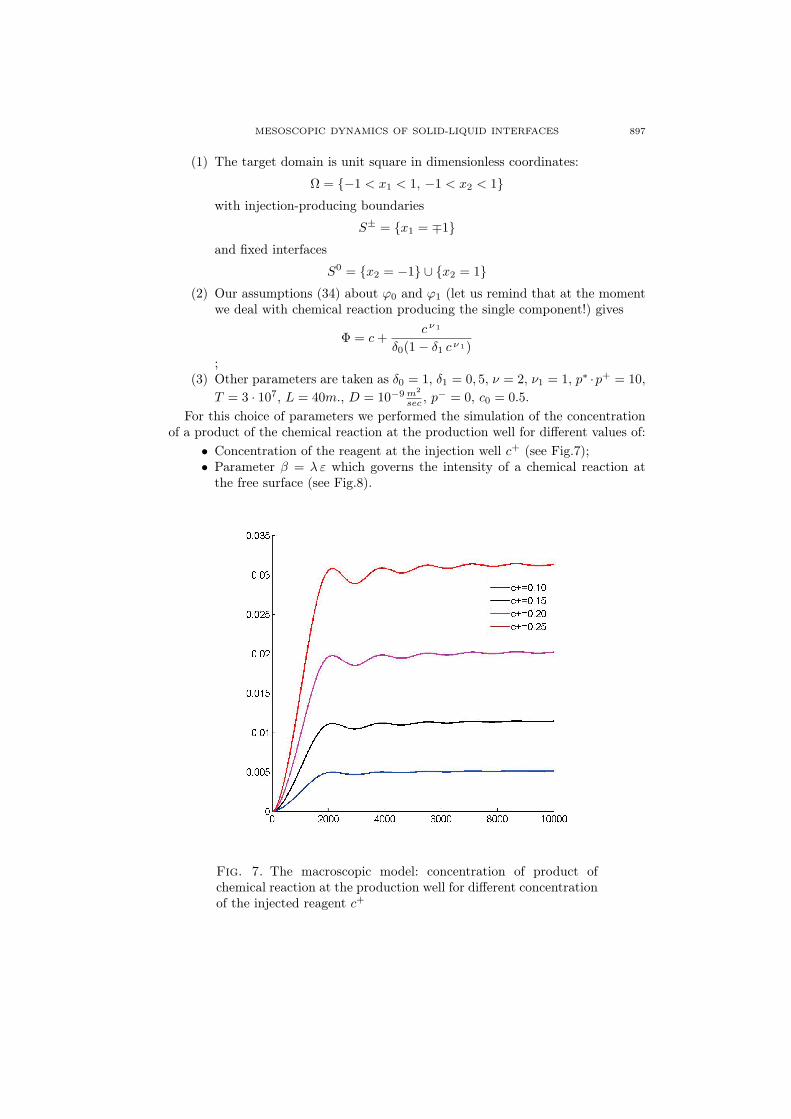
S0 = x2 = −1 ∪ x2 = 1(2) Our assumptions (34) about φ0 and φ1 (let us remind that at the moment

we deal with chemical reaction producing the single component!) gives

Φ = c+c ν 1

δ0(1− δ1 c ν 1);

(3) Other parameters are taken as δ0 = 1, δ1 = 0, 5, ν = 2, ν1 = 1, p∗ ·p+ = 10,T = 3 · 107, L = 40m., D = 10−9 m2

sec , p− = 0, c0 = 0.5.

For this choice of parameters we performed the simulation of the concentrationof a product of the chemical reaction at the production well for different values of:

• Concentration of the reagent at the injection well c+ (see Fig.7);• Parameter β = λ ε which governs the intensity of a chemical reaction at

the free surface (see Fig.8).

Fig. 7. The macroscopic model: concentration of product ofchemical reaction at the production well for different concentrationof the injected reagent c+


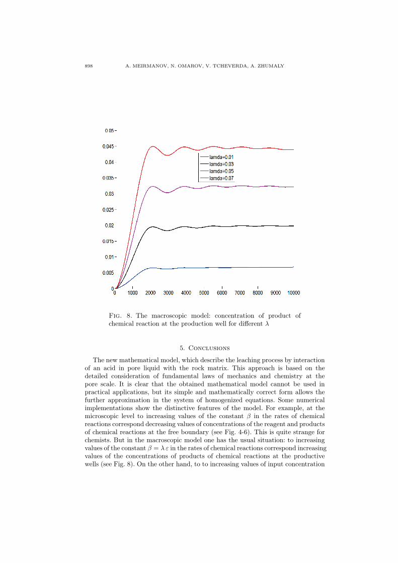
Fig. 8. The macroscopic model: concentration of product ofchemical reaction at the production well for different λ

5. Conclusions

The new mathematical model, which describe the leaching process by interactionof an acid in pore liquid with the rock matrix. This approach is based on thedetailed consideration of fundamental laws of mechanics and chemistry at thepore scale. It is clear that the obtained mathematical model cannot be used inpractical applications, but its simple and mathematically correct form allows thefurther approximation in the system of homogenized equations. Some numericalimplementations show the distinctive features of the model. For example, at themicroscopic level to increasing values of the constant β in the rates of chemicalreactions correspond decreasing values of concentrations of the reagent and productsof chemical reactions at the free boundary (see Fig. 4-6). This is quite strange forchemists. But in the macroscopic model one has the usual situation: to increasingvalues of the constant β = λ ε in the rates of chemical reactions correspond increasingvalues of the concentrations of products of chemical reactions at the productivewells (see Fig. 8). On the other hand, to to increasing values of input concentration


c+ always correspond increasing values of the concentrations of products of chemicalreactions at the free boundary in the microscopic model (see Fig. 4-6), and increasingvalues of the concentrations of products of chemical reactions at the productive wells(see Fig. 7).

Note also, that in the introduction we discussed the possibility of oscillationsfor the microscopic model. Unfortunately we cannot find these oscillations in ournumerical implementations for the microscopic model maybe because they are toosmall and to see them one needs to perform computations with much more precision.But at the macroscale these oscillations are evident and in the nearest future weplan to perform a special series of numerical experiments to understand the processin the greater details.

References

[1] F. Golfier, C. Zarcone, B. Bazin, R. Lenormand, D. Lasseux and M. Quintard, On the abilityof a Darcy-scale model to capture wormhole formation during the dissolution of a porousmedium, J. Fluid Mech., 457 (2002), 213–254. Zbl 1016.76079

[2] Kalia Nitika, Balakotaiah Vemuri, Effect of medium heterogeneities on reactive dissolutionof carbonates, Chemical Engineering Science, 64 (2009), 376–390.

[3] C.E. Cohen, D. Ding, M. Quintard, B. Bazin, From pore scale to wellbore scale: Impact ofgeometry on wormhole growth in carbonate acidization, Chemical Engineering Science, 63(2008), 3088 – 3099.

[4] M.K.R. Panga, M. Ziauddin, V. Balakotaiah, Two-scale continuum model for simulation ofwormholes incarbonate acidization, A.I.Ch.E.Journal, 51 (2005), 3231–3248.

[5] R. Burridge and J. B. Keller, Poroelasticity equations derived from microstructure, Journalof Acoustic Society of America 70:4 (1981), 1140–1146. Zbl 0519.73038

[6] E. Sanchez-Palencia, Non-Homogeneous Media and Vibration Theory, Lecture Notes inPhysics, 129, Springer-Verlag, New York, 1980. MR0578345

[7] D. Lukkassen, G. Nguetseng, P. Wall, Two-scale convergence, Int. J. Pure and Appl. Math.2:1 (2002), 35–86. MR1912819

[8] A. Meirmanov, Mathematical models for poroelastic flows, Atlantis Press, Paris, 2013.[9] A. Meirmanov, Nguetseng’s two-scale convergence method for filtration and seismic acoustic

problems in elastic porous media, Siberian Mathematical Journal, 48:3 (2007), 519–538.MR2347913

[10] A. Meirmanov, A description of seismic acoustic wave propagation in porous media viahomogenization, SIAM J. Math. Anal., 40:3 (2008), 1272–1289. MR2452887

[11] A. Meirmanov, Double porosity models in incompressible poroelastic media, MathematicalModels and Methods in Applied Sciences, 20:4 (2010), 635–659.

[12] A. Meirmanov, The Muskat problem for a viscoelastic filtration, Interfaces and FreeBoundaries, 13:4 (2011), 463–484.

[13] A. Meirmanov, The Stefan Problem, Walter de Gruyter, Berlin-New York, 1992. MR1154310[14] L.E. Malvern, Introduction to Mechanics of a Continuum Medium, Prentice–Hall, Inc.

Englewood Cliffs, N.J., 1969.[15] G.B. Whitham, Linear and nonlinear waves, Willey, ISBN 978-0-471-94090-6 (1999).

MR1699025

A.MeirmanovAl-Farabi Kazakh National UNiversity,pr. Abai, 71,050040, Almaty, KazakhstanE-mail address: [email protected]

N.OmarovKazakh-British Technical University,Abai av., 59Almaty, KazakhstanE-mail address: [email protected]


V.TcheverdaKazakh-British Technical University,Abai av., 59Almaty, Kazakhstan

A.ZhumalyKazakh-British Technical University,Abai av., 59Almaty, KazakhstanE-mail address: [email protected]

Documents

S⃝e MR - semr.math.nsc.rusemr.math.nsc.ru/v12/p884-900.pdf · MESOSCOPIC DYNAMICS OF SOLID-LIQUID INTERFACES. A GENERAL MATHEMATICAL MODEL A. MEIRMANOV, N. OMAROV, V. TCHEVERDA,