Embed Size (px)
Citation preview

Safe and Interactive Autonomy: Control, Learning, and Verification
by
Dorsa Sadigh
A dissertation submitted in partial satisfaction of the
requirements for the degree of
Doctor of Philosophy
in
Engineering - Electrical Engineering and Computer Sciences
in the
Graduate Division
of the
University of California, Berkeley
Committee in charge:
Professor Sanjit A. Seshia, Co-chairProfessor S. Shankar Sastry, Co-chair
Professor Francesco BorrelliProfessor Anca D. Dragan
Summer 2017

Safe and Interactive Autonomy: Control, Learning, and Verification
Copyright 2017by
Dorsa Sadigh
1
Abstract
Safe and Interactive Autonomy: Control, Learning, and Verification
by
Dorsa Sadigh
Doctor of Philosophy in Engineering - Electrical Engineering and Computer Sciences
University of California, Berkeley
Professor Sanjit A. Seshia, Co-chair
Professor S. Shankar Sastry, Co-chair
The goal of my research is to enable safe and reliable integration of human-robot systemsin our society by providing a unified framework for modeling and design of these sys-tems. Today’s society is rapidly advancing towards autonomous systems that interactand collaborate with humans, e.g., semiautonomous vehicles interacting with drivers andpedestrians, medical robots used in collaboration with doctors, or service robots interact-ing with their users in smart homes. The safety-critical nature of these systems require usto provide provably correct guarantees about their performance. In this dissertation, wedevelop a formalism for the design of algorithms and mathematical models that enablecorrect-by-construction control and verification of human-robot systems.
We focus on two natural instances of this agenda. In the first part, we study interaction-aware control, where we use algorithmic HRI to be mindful of the effects of autonomoussystems on humans’ actions, and further leverage these effects for better safety, efficiency,coordination, and estimation. We further use active learning techniques to update andbetter learn human models, and study the accuracy and robustness of these models. In thesecond part, we address the problem of providing correctness guarantees, while takinginto account the uncertainty arising from the environment or human models. Throughthis effort, we introduce Probabilistic Signal Temporal Logic (PrSTL), an expressivespecification language that allows representing Bayesian graphical models as part ofits predicates. Further, we provide a solution for synthesizing controllers that satisfytemporal logic specifications in probabilistic and reactive settings, and discuss a diagnosisand repair algorithm for systematic transfer of control to the human in unrealizablesettings. While the algorithms and techniques introduced can be applied to many human-robot systems, in this dissertation, we will mainly focus on the implications of my workfor semiautonomous driving.

i
To Maman, Baba, Gelareh, Amir, Vivian,and Nima.

ii
Contents
Contents ii
1 Introduction 11.1 Thesis Approach . . . . . . . . . . . . . . . . . . . . . . . . . . . . . . . . . . 21.2 Contributions . . . . . . . . . . . . . . . . . . . . . . . . . . . . . . . . . . . . 31.3 Overview . . . . . . . . . . . . . . . . . . . . . . . . . . . . . . . . . . . . . . . 8
2 Preliminaries 142.1 Formalism for Human-Robot Systems . . . . . . . . . . . . . . . . . . . . . . 142.2 Inverse Reinforcement Learning . . . . . . . . . . . . . . . . . . . . . . . . . 172.3 Synthesis from Temporal Logic . . . . . . . . . . . . . . . . . . . . . . . . . . 192.4 Simulations . . . . . . . . . . . . . . . . . . . . . . . . . . . . . . . . . . . . . . 23
I Interaction-Aware Control 26
3 Leveraging Effects on Human Actions 273.1 Human-Robot Interaction as a Two-Player Game . . . . . . . . . . . . . . . . 273.2 Approximate Solution as an Underactuated System . . . . . . . . . . . . . . 293.3 Case Studies with Offline Estimation . . . . . . . . . . . . . . . . . . . . . . . 323.4 User Study with Offline Estimation . . . . . . . . . . . . . . . . . . . . . . . . 363.5 Chapter Summary . . . . . . . . . . . . . . . . . . . . . . . . . . . . . . . . . . 41
4 Active Information Gathering over Human Internal State 434.1 Extension to Online Estimation of the Human Model . . . . . . . . . . . . . 454.2 Case Studies with Online Estimation . . . . . . . . . . . . . . . . . . . . . . . 474.3 User Study with Online Estimation . . . . . . . . . . . . . . . . . . . . . . . . 564.4 Chapter Summary . . . . . . . . . . . . . . . . . . . . . . . . . . . . . . . . . . 59
5 Active Preference-Based Learning of Reward Functions 625.1 Preference-Based Learning Problem . . . . . . . . . . . . . . . . . . . . . . . 635.2 Learning Reward Weights from Preferences of Synthesized Queries . . . . . 645.3 Synthesizing Queries through Active Volume Removal . . . . . . . . . . . . 65

iii
5.4 Algorithm and Performance Guarantees . . . . . . . . . . . . . . . . . . . . . 685.5 Simulation Experiment . . . . . . . . . . . . . . . . . . . . . . . . . . . . . . . 695.6 Usability Study . . . . . . . . . . . . . . . . . . . . . . . . . . . . . . . . . . . 745.7 Chapter Summary . . . . . . . . . . . . . . . . . . . . . . . . . . . . . . . . . . 77
6 Falsification for Human-Robot Systems 796.1 Running Example . . . . . . . . . . . . . . . . . . . . . . . . . . . . . . . . . . 806.2 Falsification in Interaction-Aware Control . . . . . . . . . . . . . . . . . . . . 816.3 Learning the Error Bound δ . . . . . . . . . . . . . . . . . . . . . . . . . . . . 846.4 Case Studies . . . . . . . . . . . . . . . . . . . . . . . . . . . . . . . . . . . . . 886.5 Chapter Summary . . . . . . . . . . . . . . . . . . . . . . . . . . . . . . . . . . 91
II Safe Control 92
7 Reactive Synthesis for Human-Robot Systems 937.1 Running Example . . . . . . . . . . . . . . . . . . . . . . . . . . . . . . . . . . 967.2 Formal Model of Human-Robot Controller . . . . . . . . . . . . . . . . . . . 977.3 Human-Robot Controller Synthesis . . . . . . . . . . . . . . . . . . . . . . . . 997.4 Experimental Results . . . . . . . . . . . . . . . . . . . . . . . . . . . . . . . . 1047.5 Chapter Summary . . . . . . . . . . . . . . . . . . . . . . . . . . . . . . . . . . 105
8 Reactive Synthesis from Signal Temporal Logic 1078.1 MILP Encoding for Controller Synthesis . . . . . . . . . . . . . . . . . . . . . 1098.2 STL Reactive Synthesis Problem . . . . . . . . . . . . . . . . . . . . . . . . . . 1118.3 Counterexample-Guided Finite Horizon Synthesis . . . . . . . . . . . . . . . 1118.4 Receding Horizon Controller Synthesis in an Adversarial Environment . . 1178.5 Autonomous Driving in Nondeterministic Environments . . . . . . . . . . . 1198.6 Chapter Summary . . . . . . . . . . . . . . . . . . . . . . . . . . . . . . . . . . 121
9 Safe Control under Uncertainty 1239.1 Bayesian Classification to Model Uncertainty: . . . . . . . . . . . . . . . . . . 1259.2 Probabilistic Controller Synthesis Problem . . . . . . . . . . . . . . . . . . . 1269.3 Experimental Results . . . . . . . . . . . . . . . . . . . . . . . . . . . . . . . . 1339.4 Chapter Summary . . . . . . . . . . . . . . . . . . . . . . . . . . . . . . . . . . 139
10 Diagnosis and Repair for Synthesis from Signal Temporal Logic 14010.1 Mixed Integer Linear Program Formulation . . . . . . . . . . . . . . . . . . . 14210.2 Running Example . . . . . . . . . . . . . . . . . . . . . . . . . . . . . . . . . . 14410.3 Diagnosis and Repair Problem . . . . . . . . . . . . . . . . . . . . . . . . . . 14510.4 Monolithic Specifications . . . . . . . . . . . . . . . . . . . . . . . . . . . . . . 14710.5 Contracts . . . . . . . . . . . . . . . . . . . . . . . . . . . . . . . . . . . . . . . 15610.6 Case Studies . . . . . . . . . . . . . . . . . . . . . . . . . . . . . . . . . . . . . 160

iv
10.7 Chapter Summary . . . . . . . . . . . . . . . . . . . . . . . . . . . . . . . . . . 165
11 Final Words 16611.1 Challenges in Safe and Interactive AI . . . . . . . . . . . . . . . . . . . . . . 16711.2 Closing Thoughts . . . . . . . . . . . . . . . . . . . . . . . . . . . . . . . . . . 171
Bibliography 172

v
Acknowledgments
I would like to first and foremost thank my advisors Sanjit Seshia and Shankar Sastry.Sanjit’s enthusiasm and perceptiveness was what drew me to research in the first place.His patience and ability to see the positive in every bit of academia has motivated methroughout the past 7 years, and I would not have been where I am today without hishelp and support. I have also been fortunate to have Shankar’s invaluable guidancethroughout my Ph.D. Every word in a conversation with Shankar is a lifelong advice,and I am grateful that he took a chance on me after my elevator pitch in the elevator ofSutardja-Dai Hall in 2012.
Many of my recent work has been in close collaboration with Anca Dragan. Overthe short time that Anca has been at Berkeley, she has given me a unique viewpoint onresearch and life. Anca has taught me how to be caring and compassionate at the sametime as being candid and constructive. I now know there is so much love in it when shesays “That was horrible!"
I would also like to thank the faculty who helped shape my research path during mytime at Berkeley. Babak Ayazifar for introducing me to the world of research. EdwardLee, my undergraduate research advisor, for letting me hang out with his group andlearn about model-based design. Ruzena Bajcsy for teaching me how to keep myselfgrounded and be my own critic. Claire Tomlin and Alberto Sangiovanni-Vincentelli fortheir support, advice, and constructive discussions. Jeannette Wing, Eric Horvitz, andAshish Kapoor for fruitful conversations that shaped my research during the awesomesummer of 2014 in Redmond.
I would also like to thank all my co-authors and collaborators, specially peoplewho helped with the work of this dissertation: Shromona Ghosh and Pierluigi Nuzzofor the awesome nights in DOP center, Nick Landolfi, Wenchao Li, Alexandre Donze,Vasumathi Raman, and Richard Murray whose ideas have helped with various parts ofthis dissertation.
Special thanks to all my mentors for letting me follow them around for a good chunkof my graduate school: Sam Burden for his wisdom, advice, and being there for all theyounger folks in the group, Joh Kotker for slowly guiding me towards formal methods,Lillian Ratliff, Dan Calderon, Roy Dong, Aaron Bestick, Katherine Driggs-Campbell, andSam Coogan for their continuing support, all the lunches, conferences, tea times, andhikes.
I also want to thank the people of TRUST, and Learn and Verify group for the fruitfulconversations over the years: Rohit Sinha, Eric Kim, Ankush Desai, Daniel Fremont, BenCaulfield, Marcell Vazquez-Chanlatte, Jaime Fisac, Dexter Scobee, Oladapo Afolabi, EricMazumdar, Tyler Westenbroek, Zach Wasson, Wei-Yang Tan, Markus Rabe, TommasoDreossi, Robert Matthew, Victor Shia, Indranil Saha, Ruediger Ehlers, Yi-Chin Wu, SusmitJha, Bryan Brady, Dan Holcomb, Nikhil Naikal, Nishant Totla, and Garvit Juniwal.
I wouldn’t be able to go through the interview season this past year without the helpand unsparing advice of Ramtin Pedarsani, Yasser Shoukry, and Justine Sherry.

vi
Many thanks to special people of TRUST and DOP center, who made everything runsmoothly: Jessica Gamble, Carolyn Winter, Mary Stewart, Larry Rohrbough, ChristopherBrooks, Annie Ren, Aimee Tabor, Shirley Salanio, and Shiela Humphreys.
I have had some of the most wonderful years of my life at Berkeley, and I owe thatto my awesome and supportive friends: Zhaleh Amini, Nazanin Pajoom, Negar Mehr,Ramtin Pedarsani, Payam Delgosha, Sana Vaziri, Hedyeh Ahmadi, Sina Akhbari, FarazTavakoli, and Yasaman Bahri.
I wanted to thank my family. My parents for all their sacrifices, love, and support. Mysister, Gelareh, for listening to my ‘ghors’ almost everyday since the day I can remember,and for constantly pushing me to go beyond my comfort zone. Special thanks to AmirRazavi, Vivian Razavi, Babak Sadigh, and Minoo Bahadori for being an important part ofmy life.
The final thanks goes to Nima Anari for making my life more enjoyable and excitingthan it has ever been. His ‘kari nadare ke!’ has made me believe in myself; his genius hasled me to look at the world differently, and his peacefulness is my endless comfort.

1
Chapter 1
Introduction
Today our society is rapidly advancing towards autonomous systems that interact andcollaborate with humans, e.g., semiautonomous vehicles interacting with drivers andpedestrians, medical robots used in collaboration with doctors, or service robots interact-ing with their users in smart homes. Humans play a central role in such autonomoussystems. They are either part of the environment that interacts with autonomy, part of thecontrol algorithm that provides the policy for the overall system, or have a supervisoryrole. For instance, in autonomous driving, the autonomous vehicle inevitably interactswith humans both inside and outside of the vehicle. The car needs to interact withthe driver inside of the vehicle, who might at times take over and steer the vehicle ina shared autonomy setting. We see this in lane keeping systems, where the controllerdecides to bring a distracted driver back into the lane. We also see it in autonomoushighway driving, when the vehicle asks the person to take over control as the highwayends. Similarly, autonomous cars will not drive in an isolated space. They will need tointeract with everything else that lives in the environment. This includes the pedestriansor human-driven vehicles around them. For example, the human driver in the nextlane of an autonomous car, might decide to slow down or speed up, when she sees anautonomous vehicle. Her actions are simply based on her model of the autonomous car’sdriving and her interaction with the autonomous car. On the other hand, the actions of theautonomous car is based on its model and interaction with the human. The autonomouscar might decide that the human is distracted, so its safest strategy is to not change lanes.The autonomous car might also decide to nudge in a bit into the next lane to initiate aninteraction, which can potentially affect the human driver (if attentive) to slow down,making some room for the autonomous car to merge in the front. In all these settings, itis crucial to understand the interaction between the human and the rest of the system,which further requires representative models of the humans’ behavior. We refer to thesesystems as human-robot systems, or interchangeabily as human-cyber-physical systems(h-CPS). These are cyber-physical systems (CPS) since they unite the physical processeswith the cyber-world, and they are h-CPS as they have a human as part of their plant,control loop, or environment interacting with them.

CHAPTER 1. INTRODUCTION 2
As these autonomous systems enter the humans’ world, their continuing interactionresults in many safety concerns. These systems don’t live in a vacuum, and their actionshave direct consequence on the environment the humans live in. In addition, these actionshighly depend on learned models of the environment or the humans they interact with. Sorobots can easily unhinge humans’ safety by relying on inaccurate models that are learnedfrom data. The safety-critical nature of these human-robot systems demands providingprovably correct guarantees about their actions, models, control, and performance. Thisbrings us to a set of fundamental problems we would like to study for human-robotsystems. How do we model humans? How do we model the interaction between thehuman and the robot? How do we leverage the growing amount of data in the design ofhuman-CPS in a principled manner? What mathematical models are suitable for formalanalysis and design of human-robot systems? How do we address safety in reactive,high-dimensional, probabilistic environments? How do we recover in the case of anunsafe event?
1.1 Thesis Approach
One of the key aspects for achieving safe controllers for human-robot systems is thedesign of the interaction between the human and autonomy. This is usually overlookedby assuming humans act as external disturbances just like moving obstacles. Humans arenot simply a disturbance that needs to be avoided; they are intelligent agents with approximatelyrational strategies. To model and control any human-robot systems, we are required todevelop verifiable models of humans, understand the interaction between them and theother agents, and leverage this interaction in construction of safe and efficient controllers.For the design of safe controllers, we further need to formally express the desirableproperties the human-robot system should satisfy, and only then we can construct astrategy for the robot that would satisfy the formalism.
In order to address safety and interaction, we divide this dissertation into two partsfirst focusing on interaction-aware control, and then discussing safe control.
Our approach in interaction-aware control is to model the interaction between thehuman and the robot as an underactuated dynamical system, where the actions of therobot can influence the actions of the human. We assume the human and the robot arereward maximizing agents. We further study the human’s reward function by:
(i) actively updating the reward function in online manner to address the deviationfrom different people’s behaviors;
(ii) actively synthesizing comparison queries to learn human’s preference reward func-tions, and
(iii) verifying the safety of the overall system by disturbance analysis of the learnedreward function.

CHAPTER 1. INTRODUCTION 3
This disturbance analysis is a step towards addressing the safety of the overall human-robot system while using learned models, which brings us to the discussion of safecontrol.
We take a formal methods approach to address the safety question, where we formalizethe desired specifications as temporal logic properties. We then design controllers thatwould either satisfy the specification, or in the case that such controllers do not exist, theywould systematically diagnose the failure, transfer control to the human (or some othersupervisor), and even provide suggested repairs for the specifications. We study differenttypes of specifications to address continuity and stochasticity present in human-robotsystems.
Here, we bridge ideas from formal methods, control theory, and human-robot interac-tion to understand and design controllers that are interactive, can influence people, andcan guarantee to satisfy high level properties such as safety.
1.2 Contributions
This thesis makes the following contributions.
The goal of my thesis is to develop a safe and interactive control framework for human-robot systems.
Planning for Robots to Coordinate with Other People:
We provide a formalism for interaction between a human and a robot as a partiallyobservable two-player game. The human and the robot can both act to change the stateof the world, and they have partial information because they don’t know each others’reward functions. We model the human as an agent who is approximately optimizingher reward function learned through demonstrations [129, 3, 188, 107], and the robot as arational agent optimizing its own reward function.
This formulation has two issues: intractability, especially in continuous state andaction spaces, and failing to capture human behavior, because humans tend to not followNash equilibria in day to day tasks [76]. We introduce a simplification of this formulationto an underactuated system. We assume that the robot decides on a trajectory uR, andthe human computes a best response to uR (as opposed to trying to influence uR aswould happen in a game).
In addition, we derive an approximate solution for our system based on ModelPredictive Control and a quasi-newton optimization. At every step, the robot replansa trajectory uR by reasoning about the optimization that the human would do basedon a candidate uR. We use implicit differentiation to obtain a gradient of the human’strajectory with respect to the robot’s. This enables the robot to compute a plan in close toreal-time. We evaluate our algorithm through a user study in an autonomous driving

CHAPTER 1. INTRODUCTION 5
scenario, which suggests that robots are capable of affecting human’s actions and drivingthem to a desired state (Chapter 3) [159, 160].
Active Information Gathering over Human’s Internal State:
Our human-robot interaction model depends on accurate estimations of human rewardfunction. This can be done by estimating the human reward offline from training data,but ultimately every driver is different, and even the same driver is sometimes moreor less aggressive, more or less attentive, and so on. We thus explore estimating thehuman reward function online. This turns the problem into a partially observable Markovdecision process (POMDP), with the human reward parameters as the hidden state.Prior work that incorporates some notion of human state into planning has thus farseparated estimation and planning, always using the current estimate of the humanstate to determine what the robot should do [81, 58, 18]. Although efficient, theseapproximations sacrifice an important aspect of POMDPs: the ability to actively gatherinformation.
We take advantage of the underactuated system to gather information about thehuman reward parameters. Rather than relying on passive observations, the robot actuallyaccounts for the fact that humans will react to their actions: it uses this knowledge toselect actions that will trigger human reactions which in turn will clarify the internal state.We apply our algorithm to estimating a human driver’s style during the interaction withan autonomous vehicle, and our results in simulation and a user study suggest that ouralgorithm is capable of leveraging robot’s actions for estimation that leads to significantlyhigher accuracy in identifying the correct human internal state (Chapter 4) [158, 160].
Active Preference-Based Learning of Reward Functions:
Reward functions play a central role in specifying how dynamical systems should act.For many systems, human’s have a difficult time providing demonstrations of what theywant. We propose a preference-based approach to learning desired reward functions in adynamical system. Instead of asking for demonstrations, or for the value of the rewardfunction for a sample trajectory (e.g., “rate the safety of this driving maneuver from 1 to10”), we ask people for their relative preference between two sample trajectories (e.g., “isξ1 more safe or less safe than ξ2?”).
We provide an algorithm for actively synthesizing such comparison queries from scratch.Our algorithm uses continuous optimization in the query space to maximize the expectedvolume removed from the hypothesis space. The human’s response assigns weightsto the hypothesis space in the form of a log-concave distribution, which provides anapproximation of the objective. We provide a bound on the number of iterations requiredto converge. In addition, we show that our algorithm converges faster than non-activeand non-synthesis techniques in learning the reward function in an autonomous driving

CHAPTER 1. INTRODUCTION 6
setting. We illustrate the performance of our algorithm in terms of accuracy of the rewardfunction learned through an in-lab usability study (Chapter 5) [156].
Falsification for Human-Robot Systems:
Safe and interactive human-robot systems strongly depend on reliable models of humanbehavior. It is crucial to be able to formally analyze such human models (e.g. learnedreward functions) to address the safety and robustness of the overall system. We providea new approach for rigorous analysis of human-robot systems that are based on learnedmodels of human behavior. We formalize this problem as a constrained optimization,where we examine the existence of a falsifying controller for the human that lies withina bounded region of the learned model and could possibly lead to unsafe outcomes.For instance, in a driving scenario, we find a sequence of possible human actions thatpotentially leads to a collision between the vehicles. We reduce this optimization to amore efficiently-solvable problem with linear constraints. In addition, we provide anefficient (almost linear time) optimization-driven approach to estimate the error boundbetween the true human reward function and the controller’s estimate. We evaluate ourtechnique for an autonomous driving example, where we find such falsifying actionswithin the learned safety bound (Chapter 6) [155].
Reactive Synthesis for Human-Robot Systems:
We formalize the problem of safe control for human-robot systems as a reactive synthesisproblem [139]. We consider a shared control setting, where either the human or therobot can operate the system, and we provide controllers that are guaranteed to satisfya set of high level specifications. Our algorithm satisfies four criteria for the overallsystem: i) monitoring: the robot determines if any human intervention is required basedon monitoring the environment. ii) minimal intervention: the robot asks for humanintervention only if it is necessary. iii) prescient: the robot determines if a specificationis going to be violated ahead of time to give enough takeover time to the human basedon the human’s reaction time. iv) conditional correctness: the robot satisfies the high levelspecification until when the human needs to intervene.
We use a discrete state and action model of the robot to be able to guarantee satisfactionof high level Linear Temporal Logic (LTL) specifications. We leverage counterstrategygraphs in our algorithm to formalize the intervention problem. Based on the four desiredcriteria, our algorithm finds a s-t minimum cut of the counterstrategy graph to determinewhen the human needs to takeover. We only monitor the human’s reaction time aspart of the human model; however, our algorithm is able to automatically find theenvironment assumptions that need to be monitored and systematically transfers controlto the human if it can’t guarantee satisfaction of the high level specifications. We showcaseour algorithm for a system motivated by driver-assistance systems (Chapter 7) [110].

CHAPTER 1. INTRODUCTION 7
Reactive Synthesis from Signal Temporal Logic
Reactive synthesis from LTL is a powerful technique that enables us to provide correctnessguarantees for autonomous systems. However, using LTL requires a discrete state andaction dynamical system. Such discretization is not very realistic for many robotics andcontrol applications as they are usually inherently continuous. So instead, we formalizethe problem of reactive synthesis from Signal Temporal Logic (STL), a specificationlanguage that is defined over continuous time and real-valued signals. Synthesizingreactive controllers under STL allows us to provide correctness guarantees even when weare dealing with continuous state and action dynamical systems.
We provide a new algorithm using ideas from counterexample-guided inductive synthesis(CEGIS) [166]. We solve a series of counterexample-guided optimization problems thatresult in finding a controller that satisfies the given STL specifications in a recedinghorizon fashion. We demonstrate the effectiveness of our algorithm in a driving examplewith a simple adversarial model of other human-driven vehicles. Similar to [146], we relyon transforming STL specifications to mixed integer linear program (MILP) encodings.Our method is a fundamentally novel approach to reactive synthesis for hybrid systems,different from most current methods, which often rely on model transformations, e.g.,abstraction and discretization (Chapter 8) [149].
Safe Control under Uncertainty
As powerful as STL specifications are, they do not have the capability of encodingstochastic properties that can arise in human-robot systems. The desired properties inmany robotics applications are based on the output of estimation and learning algorithms.For instance, safe control of a flying quadrotor depends on how certain the estimationalgorithm is about the location of the other agents in the environment including thehuman agents. This is based on the current sensor data and specific classification methodsbeing used.
We formally define a specification language to address the safe control of robotsunder such uncertain environment or human models. Probabilistic Signal Temporal Logic(PrSTL) is our specification language that enables expressing probabilistic properties,which can embed Bayesian graphical models. This probabilistic logical specificationlanguage enables reasoning about safe control strategies by embedding various predic-tions and their associated uncertainty. Furthermore, we solve a receding horizon controlproblem to satisfy PrSTL specifications using mixed integer semidefinite programs. Weshowcase our algorithm for examples in autonomous driving and control of quadrotorsin uncertain environments (Chapter 9) [154].

CHAPTER 1. INTRODUCTION 8
Diagnosis and Repair for Synthesis from Signal Temporal Logic
When synthesizing safe controllers that satisfy high level specifications such as LTL,STL, or PrSTL, we usually transform the problem to a game (in the case of LTL), or anoptimization (in the case of STL and PrSTL), and use existing techniques to solve fora safe control strategy. However, there could be situations where there does not exista controller that satisfies all the given specifications. In this context, an unrealizableSTL specification leads to an infeasible optimization problem. We leverage the abilityof existing mixed integer linear programming (MILP) solvers to localize the cause ofinfeasibility to so-called Irreducibly Inconsistent Systems (IIS). We propose an algorithmthat uses the IIS to localize the cause of unrealizability to the relevant parts of the STLspecification. Additionally, we give a method for generating a minimal set of repairs to theSTL specification such that, after applying those repairs, the resulting specification isrealizable. The set of repairs is drawn from a suitably defined space that ensures that werule out vacuous and other unreasonable adjustments to the specification. Our algorithmsare sound and complete, i. e., they provide a correct diagnosis, and always terminate witha reasonable specification that is realizable using the chosen synthesis method, whensuch a repair exists in the space of possible repairs.
1.3 Overview
Interaction-Aware Control
Effects on Human Actions. Safe and interactive human-robot systems requires modelingthe human, and taking into account the interaction that weaves the agents together. Forinstance, currently autonomous cars tend to be overly defensive and obliviously opaque.When needing to merge into another lane, they will patiently wait for another driver topass first. When stopped at an intersection and waiting for the driver on the right togo, they will sit there unable to wave them by. They are very capable when it comes toobstacle avoidance, lane keeping, localization, active steering and braking [170, 108, 56,55, 54, 44, 106]. But when it comes to other human drivers, they tend to rely on simplisticmodels: for example, assuming that other drivers will be bounded disturbances [71, 149],they will keep moving at the same velocity [175, 118, 154], or they will approximatelyfollow one of a set of known trajectories [174, 77].
These models predict the trajectory of other drivers as if those drivers act in isolation.They reduce human-robot interaction to obstacle avoidance: the autonomous car’s task isto do its best to stay out of the other drivers’ way. It will not nudge into the lane to test ifthe other driver yields, nor creep into the intersection to assert its turn for crossing.
Our insight is that the actions of an autonomous car affect the actions of other drivers,and leveraging these effects in planning improves efficiency and coordination.


CHAPTER 1. INTRODUCTION 10
Decision Process (POMDP), where the human’s internal state denotes the unobservedvariable. We augment the robot’s reward function with an exploration term (i.e. entropyover the belief of the human’s internal state), which results in a strategy for the robotthat actively takes actions to improve its estimate. Exploration actions emerge outof optimizing for information gain, such as the robot nudging into the other lane andresponding safely (going back to its lane or completing the merge) if the human driver isdistracted or attentive respectively (Figure 1.2(d)) [158, 160].Active Preference Based Learning of Reward Functions. Most of our work in interaction-aware control depends on acquiring representative models of human behaviors suchas their reward functions. Efficiently learning reward functions that encode humans’preferences for how a dynamical system should act results in various challenges. It is quitedifficult for people to demonstrate trajectories for robots with more than a few degrees offreedom or even to provide labels for precisely how much reward an action or trajectoryshould get, like a robot motion or a driving maneuver. Moreover, the learned rewardfunction strongly depends on what environments and trajectories were experiencedduring the training phase. Our approach to efficiently learn human’s preference rewardfunctions is by actively synthesizing comparison queries that human’s can respond to,and use ideas from volume-maximization and adaptive submodular optimization toactively synthesize such queries, which allow us to quickly converge to human’s rewardfunction [156].Measuring Human Variations. Since many human-robot systems are emerging into ourevery day lives, we are required to understand and measure their performance and safeinteraction in this environment. For instance, our framework depends on the quality ofthe learned human models, e.g., we would like to analyze how good of a reward functionwe have learned. Under the assumption that humans are approximately rational, we caneither use the principle of maximum entropy to learn such reward functions, as we doin [159, 158, 160], or apply our active preference-based learning technique to quicklyconverge to human’s preference reward functions [156].
These data-driven human models such as human reward functions are usually con-structed based on large datasets that give access to a single model of rationality. However,humans vary in how they handle different situations, and we cannot fit a single modelto all humans. In safety-critical scenarios, we need to be able to quantize and measurehow humans can differ from the fitted model. As a step towards verified human modeling,we construct an efficient (almost linear, i.e., O(n log n), where n is the number of queries)algorithm to quantize and learn a distribution over the variations from the fitted modelby querying individual humans on actively generated scenarios.
Overall, this thesis takes a step towards robots that account for their effects on humanactions in situations that are not entirely cooperative, and leverage these effects tocoordinate with people. Natural coordination and interaction strategies are not hand-coded, but emerge out of planning in our model. Further, we study various models of ourreward function through comparison based learning or falsification in our human-robotsystems. The material in the first part of this thesis is based on joint work with Anca D.

CHAPTER 1. INTRODUCTION 11
Dragan, S. Shankar Sastry, and Sanjit A. Seshia [159, 158, 160, 156, 155].
Safe Control
Reactive and Stochastic Controller Synthesis from Temporal Logics. The problem ofcorrect-by-construction controller synthesis has been addressed in the area of formalmethods. We formalize a set of desired high level specification, then the realizabilityproblem is to find an autonomous strategy for the robot so no matter what the envi-ronment or the other agents, e.g., humans do, the strategy for the robot is guaranteedto satisfy the specification. Linear Temporal Logic (LTL) is a popular formalism forstating these specifications. However, there is a significant gap between the expressivityof specifications in LTL and the desired requirements in robotics applications includinghuman-robot systems.
Most of these applications deal with inherently continuous systems, and the discretenature of LTL is incapable of representing properties over continuous time and spacetrajectories. Signal Temporal Logic (STL) is a specification language that addresses someof these shortcomings by providing a language over real-valued and continuous-timesignals. However, synthesizing reactive controllers that satisfy STL specifications is achallenging problem. Previous work by Raman et al. has studied synthesizing non-reactivecontrollers under STL specifications by translating the specifications to mixed-integerlinear program (MILP) constraints [146]. As part of this thesis in collaboration withVasumathi Raman, Alexandre Donze, Richard Murray, and Sanjit A. Seshia [149], westudy the problem of reactive synthesis under STL specifications. We use a similarapproach to encode the specifications as MILPs, and leverage a series of counterexampleguided optimizations to find a controller that would satisfy the desired property underreactive specifications [149].
Even though STL addresses continuous time and real-valued specifications, it stilllacks the ability to express the stochasticity arising from the environment or the humanmodels. It would be unrealistic to assume, we deterministically know where everyagent is located. Our sensors are noisy, hence our estimation algorithms at best canprobabilistically locate every agent in the environment. To address these limitations,we introduce a new formalism, Probabilistic Signal Temporal Logic (PrSTL), which is anexpressive language that closes this gap by including machine learning techniques, namelyBayesian classifiers as part of its predicates. This is joint work done at Microsoft Research,Redmond with Ashish Kapoor [154]. We further formalize a controller synthesis problemunder satisfaction of PrSTL specifications, and solve a model predictive control problem,where the synthesized strategy would satisfy the desired PrSTL properties. We reducethis optimization to a mixed-integer second-order cone program (MISOCP) [154].Explaining Failures: Accountable Human Intervention. Synthesizing safe controllersunder stochastic or adversarial environments does not always result in feasible solutions.Sometimes the extremely safe strategy for the robot does not exist.


CHAPTER 1. INTRODUCTION 13
Overall this thesis takes a step towards the design of safe and interactive autonomouscontrollers for human-robot systems. It leverages computational models of humanbehaviors to design an interaction model between the human and robot in order toinfluence the human for better safety, efficiency, coordination, and estimation. We alsotake an effort in better designing humans’ reward functions through active preferencebased learning as well as finding a sequence of falsifying actions for the human withinan error bound of the reward function. Under such uncertain human models, we addressthe safe control problem by defining relevant specifications and synthesizing a controllerthat would satisfy such specifications using either automata-based or optimization-basedtechniques. In addition, we diagnose and repair the specifications in case of infeasibilities,which enables a systematic transfer of control to the human.


CHAPTER 2. PRELIMINARIES 15
This modeling choice addresses how the actions of the human and robot together candrive the dynamics of the system to desirable states. This would require modeling actualactions of humans in a computational setting rather than a high level behavioral modelof cognition. The model of the human should explain how the actions of the humaninfluence or gets influenced in this dynamical system.
A state x ∈ X in our system is continuous, and includes the state of the humanand robot. The robot can apply continuous controls uR, which affect state immediatelythrough a dynamics model fR:
x′ = fR(x, uR) (2.1)
However, the next state the system reaches also depends on the control the humanchooses, uH. This control affects the intermediate state through a dynamics model fH:
x′′ = fH(x′, uH) (2.2)
The overall dynamics of the system combines the two. We note that the ordering of theactions of human or robot does not matter, and we assume these control inputs are takensimultaneously:
xt+1 = fH(
fR(xt, utR), ut
H)
(2.3)
We let f denote the dynamics of such discrete-time system:
xt+1 = f (xt, utR, ut
H) (2.4)
Further, we assume the robot has a particular reward function at every time step. Therobot’s reward function depends on the current state, the robot’s action, as well as theaction that the human takes at that step in response, rR(xt, ut
R, utH). At every time step,
the robot’s actions can be explained by maximizing this reward function. We assume, thisreward function is a weighted combination of features that the robot cares about, e.g., inthe driving example such features include collision avoidance, staying on the road, ordistance to the final goal.
In Figure 2.1, imagine the orange car’s goal is to go to the left lane. So its actionswould be based on optimizing a reward function that has a term regarding distance tothe left lane, distance to the blue and white car for collision avoidance, the heading andspeed of the orange car, and its distance to the lanes or road boundaries. Ideally, theorange car would optimize such function to take safe and interactive actions towards itsgoal. It is clear that such a reward function depends on the current state of the world xt,as well as the actions of the other vehicles on the road ut
H and its own actions utR.
The key aspect of this formulation is that the robot will have a model for what uH will be, anduse that in planning to optimize its reward.
Model Predictive Control (MPC):
The robot will use Model Predictive Control (MPC) [124] (also known as RecedingHorizon Control (RHC)) at every iteration. MPC is a popular framework for the design of

CHAPTER 2. PRELIMINARIES 16
autonomous controllers since generating a closed-loop policy is intractable in a complex,nonlinear, and non-convex human-robot dynamical system. In addition, computingcontrollers for a finite horizon has the benefit of computational tractability as well asaddressing the limited range of sensors.
It will compute a finite horizon sequence of actions to maximize its reward. We reducethe computation required by planning for a shorter horizon of N time steps. We executethe control only for the first time step, and then re-plan for the next N at the next timestep [35].
Let x = (x1, . . . , xN)⊤ denote a sequence of states over a finite horizon, N, and letuH = (u1
H, . . . , uNH)⊤ and uR = (u1
R, . . . , uNR)⊤ denote a finite sequence of continuous
control inputs for the human and robot, respectively. We define RR as the robot’s rewardover the finite MPC time horizon:
RR(x0, uR, uH) =N
∑t=1
rR(xt, utR, ut
H), (2.5)
where x0 denotes the present physical state at the current iteration, and each statethereafter is obtained from the previous state and the controls of the human and robotusing the given dynamics model, f .
At each iteration, we desire to find the sequence uR which maximizes the reward ofthe robot, but this reward ostensibly depends on the actions of the human. The robotmight attempt to influence the human’s actions, and the human, rationally optimizing forher own objective, might likewise attempt to influence the actions of the robot.
u∗R = arg maxuR
RR(
x0, uR, u∗H(x0, uR))
(2.6)
Here, u∗H(x0, uR) is what the human would do over the next N steps if the robot were toexecute uR.
The robot does not actually know u∗H, but in the future sections we propose a modelfor the human behavior that the robot can use to make this problem tractable.
Similarly the robot’s actions and dynamics can be affected by other elements in theenvironment. These could be other existing agents, or simply disturbances present in theenvironment. For instance, in Figure 2.1, we can consider other vehicles on the road (e.g.blue car) that are not in close interaction with the robot as such disturbances. We canthen extend our formulation, and consider a continuous-time system Σ of the form:
x = fc(x, utR, ut
H, w)
where w ∈ W is the external input provided by the environment that can possibly beadversarial. We will refer to w as the environment input. Here, fc is the continuousdynamics of the system.
Given a sampling time ∆t > 0, we assume that Σ admits a discrete-time approximationΣd of the form:
xt+1 = f (xt, utR, ut
H, wt) (2.7)

CHAPTER 2. PRELIMINARIES 17
An infinite run
ξω = (x0, u0R, u0
H, w0)(x1, u1R, u1
H, w1)(x2, u2R, u2
H, w2)...
of Σd is a sequence of state and actions starting from the initial state x0 that followthe dynamical system f . Given x0 ∈ X and the finite sequence of actions uR, uH, andw = (w1, . . . , wN)⊤, the finite run ξ = (x0, uR, uH, w) is a unique sequence generatedfollowing equation (2.7):
ξ = (x0, uR, uH, w) = (x0, u0R, u0
H, w0)(x1, u1R, u1
H, w1), . . . , (xN, uNR, uN
H, wN) (2.8)
In addition, we introduce a generic cost function J(ξ) similar to the generic rewardfunction introduced in (2.5) for the robot RR(ξ) that maps (infinite and finite) runs to R.
2.2 Inverse Reinforcement Learning
Modeling human behavior is a challenging task that has been addressed in various fields.Our goal is to use computational models of human behaviors to be able to inform thedesign of our control algorithms for human-robot systems. Apprenticeship learningis a possible technique for constructing such computational models of humans; thelearner finds a reward function that explains observations from an expert providingdemonstrations [129, 3]. Similar to the robot’s reward function, we model H as an agentwho noisily optimizes her own reward function [188, 107, 165, 98]. We parametrize thehuman reward function as a linear combination of a set of hand-coded features:
rH(xt, utR, ut
H) = w · φ(xt, utR, ut
H) (2.9)
Here, φ(xt, utR, ut
H) is a vector of such features, and w is a vector of the weights corre-sponding to each feature. The features describe different aspects of the environmentor the robot that the human should care about. We apply the principle of maximumentropy [188, 187] to define a probability distribution over human demonstrations uH,with trajectories that have higher reward being more probable:
P(uH|x0, w) =exp(RH(x0, uR, uH))
∫
exp(RH(x0, uR, uH))duH(2.10)
We then do an optimization over the weights w in the reward function that make thehuman demonstrations the most likely:
maxw
P(uH|x0, w) (2.11)


CHAPTER 2. PRELIMINARIES 19
• φ1 ∝ c1 · exp(−c2 · d2): distance to the boundaries of the road, where d is the distancebetween the vehicle and the road boundaries and c1 and c2 are appropriate scalingfactors as shown in Figure 2.2(a).
• φ2: distance to the middle of the lane, where the function is specified similar to φ1
as shown in Figure 2.2(b).
• φ3 = (v− vmax)2: higher speed for moving forward through, where v is the velocityof the vehicle, and vmax is the speed limit.
• φ4 = βH · n: heading; we would like the vehicle to have a heading along with theroad using a feature, where βH is the heading of H, and n is a normal vector alongthe road.
• φ5 corresponds to collision avoidance, and is a non-spherical Gaussian over thedistance of H and R, whose major axis is along the robot’s heading as shownin Figure 2.2(c).
Demonstrations
We collected demonstrations of a single human driver in an environment with multipleautonomous cars, which followed precomputed routes.
Despite the simplicity of our features and robot actions during the demonstrations,the learned human model is enough for the planner to produce behavior that is human-interpretable, and that can affect human action in the desired way as discussed in thefuture chapters.
2.3 Synthesis from Temporal Logic
In the Safe Control part of this dissertation, we focus on the idea of correct-by-constructioncontrol, which enables the design of controllers that are guaranteed to satisfy variousspecifications such as safety of the human-robot system. Our work is based on the reactivesynthesis approach introduced in the area of formal methods. The idea of temporal logicsynthesis is to automatically construct an implementation that is guaranteed to satisfy abehavioral description of the system expressed in temporal logic [142]. In this section, wegive an overview on synthesizing reactive modules from a specification given in TemporalLogic. This problem originates from Church’s problem formulated in 1965 and can beviewed as a two-player game between the system and the environment.
Problem 1 (Alonzo Church’s Synthesis Problem). Given a requirement which a circuit is tosatisfy, we may suppose the requirement expressed in some suitable logistic system which is anextension of restricted recursive arithmetic.
The synthesis problem is the to find recursion equivalences representing a circuit that satis-fies the given requirement (or alternatively, to determine that there is no such circuit) [34].

CHAPTER 2. PRELIMINARIES 20
Linear Temporal Logic
Specifications are detailed descriptions of the desired properties of a system (e.g. au-tonomous agent, robot) along with its environment. We use Linear Temporal Logic(LTL) [141] to formally define such desired specifications. A LTL formula is built ofatomic propositions ω ∈ Π that are over states of the system that evaluate to True or False,propositional formulas φ that are composed of atomic propositions and Boolean operatorssuch as ∧ (and), ¬ (negation), and temporal operations on φ. Some of the common temporaloperators are defined as:
G φ φ is true all future moments.F φ φ is true some future moments.X φ φ is true the next moment.φ1 U φ2 φ1 is true until φ2 becomes true.
Using LTL, we can define interesting liveness and safety properties. For example, GF φdefines a surveillance property specifying that φ needs to hold true infinitely often. Onthe other hand, FG φ represents a stability specification by requiring φ to stay true aftera particular point in the future. Similarly G(φ → F ψ) represents a response operatormeaning that at all times if φ becomes true then at some point in the future ψ must turntrue as well.
The goal of reactive synthesis from LTL is to automatically construct a controller thatis guaranteed to satisfy the given LTL specifications. The solution to this problem iscomputed by first constructing an automaton from the given specification, which thentranslates to a two-player game between the system components and the environmentcomponents. A deterministic Rabin automaton is a formalism that enables representingLTL specifications in the form of an automaton that can then be translated to the two-player game.
Definition 1. A deterministic Rabin automaton is a tuple R = 〈Q, Σ, δ, q0, F〉 where Q isthe set of states; Σ is the input alphabet; δ : Q × Σ → Q is the transition function; q0 is theinitial state and F represents the acceptance condition: F = (G1, B1), . . . , (GnF
, BnF) where
Gi, Bi ⊂ Q for i = 1, . . . , nF.
A run of a Rabin automaton is an infinite sequence r = q0, q1 . . . where q0 ∈ Q0 andfor all i > 0, qi+1 ∈ δ(qi, σ), for some input σ ∈ Σ. For every run r of the Rabin automaton,inf(r) ∈ Q is the set of states that are visited infinitely often in the sequence r = q0, q1 . . . .A run r = q0, q1 . . . is accepting if there exists i ∈ 1, . . . , nF such that:
inf(r) ∩ Gi 6= ∅ and inf(r) ∩ Bi = ∅ (2.13)
For any LTL formula φ over Π, a deterministic Rabin automaton (DRA) can beconstructed with input alphabet Σ = 2Π that accepts all and only words over Π thatsatisfy φ [161]. We let Rφ denote this DRA.

CHAPTER 2. PRELIMINARIES 21
Intuitively, a run of the Rabin automaton is accepted if and only if it visits the accepting(good) states Gi infinitely often, and visits the non-accepting (bad) states Bi only finitelyoften. Acceptance of a run in DRA Rφ is equivalent to satisfaction of the LTL formula φby that particular run.
The solution to the reactive synthesis problem is then a winning strategy for the systemthat is extracted from this two-player game created by the DRA. Such a strategy wouldbe winning for the system under any sequence of possible environment inputs.
There also exists situations, where a winning strategy does not exist for the environ-ment, i.e., there exist an adversarial environment input sequence that can lead to theviolation of the given LTL property. In such scenarios, we instead extract a winningstrategy for the environment. Such a strategy is called a counterstrategy and providesa policy for the environment that summarizes all the possible adversarial moves theenvironment component can possibly take to drive the system to the violation of thespecification.
Signal Temporal Logic
LTL provides a rich and expressive specification language that enables formally specifyinghigh level properties of a reactive system. However, one major downside of using LTLis the need to discretize the state space, which is quite unrealistic for many roboticsand control applications that are inherently continuous. Signal Temporal Logic (STL) isanother specification language that can address some of these limitations. We considerSTL formulas defined recursively according to the grammar
ϕ ::= πµ | ¬πµ | ϕ ∧ ψ | ϕ ∨ ψ | G[a,b] ψ | ϕ U[a,b] ψ
where πµ is an atomic predicate Rn → B whose truth value is determined by the sign ofa function µ : Rn → R and ψ is an STL formula.
An interesting property of STL is its ability to express specifications for continuous-time, real-valued signals. However, in the rest of this dissertation, we focus only ondiscrete-time, real-valued signals, which is already sufficient to avoid space discretization.STL also has the advantage of naturally admitting a quantitative semantics which, inaddition to the binary answer to the question of satisfaction, provides a real numberindicating the quality of the satisfaction or violation. Such quantitative semantics havebeen defined for timed logics e.g. Metric Temporal Logic (MTL) [52] and STL [45] toassess the robustness of the systems to parameter or timing variations.
The validity of a formula ϕ with respect to the discrete-time signal ξ at time t, noted

CHAPTER 2. PRELIMINARIES 22
(ξ, t) |= ϕ is defined inductively as follows:
(ξ, t) |= πµ ⇔ µ(ξt) > 0(ξ, t) |= ¬πµ ⇔ ¬((ξ, t) |= πµ)(ξ, t) |= ϕ ∧ ψ ⇔ (ξ, t) |= ϕ ∧ (ξ, t) |= ψ(ξ, t) |= ϕ ∨ ψ ⇔ (ξ, t) |= ϕ ∨ (ξ, t) |= ψ(ξ, t) |= G[a,b]ϕ ⇔ ∀t′ ∈ [t+a, t+b], (ξ, t′) |= ϕ
(ξ, t) |= F[a,b]ϕ ⇔ ∃t′ ∈ [t + a, t + b], (ξ, t′) |= ϕ
(ξ, t) |= ϕ U[a,b] ψ ⇔ ∃t′ ∈ [t+a, t+b] s.t. (ξ, t′) |= ψ
∧∀t′′ ∈ [t, t′], (ξ, t′′) |= ϕ.
Here, ξt is the value of sequence ξ at time t. For instance if ξ is a sequence of state,action pairs as in equation (2.8), ξt = (xt, ut
R, utH, wt). A signal ξ satisfies ϕ, denoted by
ξ |= ϕ, if (ξ, t0) |= ϕ. Informally, ξ |= G[a,b]ϕ if ϕ holds at every time step between a and
b, and ξ |= ϕ U[a,b] ψ if ϕ holds at every time step before ψ holds, and ψ holds at some
time step between a and b. Additionally, we define F[a,b]ϕ = ⊤ U[a,b] ϕ, so that ξ |= F[a,b]ϕif ϕ holds at some time step between a and b.
A STL formula ϕ is bounded-time if it contains no unbounded operators; the bound of ϕis the maximum over the sums of all nested upper bounds on the temporal operators, andprovides a conservative maximum trajectory length required to decide its satisfiability.For example, for G[0,10]F[1,6] ϕ, a trajectory of length N ≥ 10 + 6 = 16 is sufficient todetermine whether the formula is satisfiable. This bound can be computed in time linearin the length of the formula.
Robust Satisfaction of STL formulas
Quantitative or robust semantics define a real-valued function ρϕ of signal ξ and t suchthat (ξ, t) |= ϕ ≡ ρϕ(ξ, t) > 0. In this work, we utilize a quantitative semantic forspace-robustness, which is defined as follows:
ρπµ(ξ, t) = µ(ξt)
ρ¬πµ(ξ, t) = −µ(ξt)
ρϕ∧ψ(ξ, t) = min(ρϕ(ξ, t), ρψ(ξ, t))ρϕ∨ψ(ξ, t) = max(ρϕ(ξ, t), ρψ(ξ, t))
ρG[a,b]ϕ(ξ, t) = mint′∈[t+a,t+b] ρϕ(ξ, t′)ρF[a,b]ϕ(ξ, t) = maxt′∈[t+a,t+b] ρϕ(ξ, t′)ρϕ U[a,b] ψ(ξ, t) = maxt′∈[t+a,t+b](min(ρψ(ξ, t′), mint′′∈[t,t′] ρϕ(ξ, t′′))
To simplify notation, we denote ρπµby ρµ for the remainder of this work. The
robustness of satisfaction for an arbitrary STL formula is computed recursively fromthe above semantics in a straightforward manner, by propagating the values of thefunctions associated with each operand using min and max operators corresponding

CHAPTER 2. PRELIMINARIES 23
to the various STL operators. For example, for a signal x = x0, x1, x2 . . . , the robustsatisfaction of πµ1 where µ1(x) = x − 3 > 0 at time 0 is ρµ1(x, 0) = x0 − 3. Therobust satisfaction of µ1 ∧ µ2 is the minimum of ρµ1 and ρµ2 . Temporal operators aretreated as conjunctions and disjunctions along the time axis: since we deal with discretetime, the robustness of satisfaction of ϕ = G[0,2]µ1 is ρϕ(x, 0) = mint∈[0,2] ρµ1(x, t) =
minx0 − 3, x1 − 3, . . . , xK − 3 where 0 ≤ K ≤ 2 < K + 1.Note that for continuous time, the min and max operations would be replaced by inf
and sup, respectively.The robustness score ρϕ(x, t) should be interpreted as how much model x satisfies ϕ.
Its absolute value can be viewed as the distance of x from the set of trajectories satisfyingor violating ϕ, in the space of projections with respect to the functions µ that define thepredicates of ϕ. In addition, the robustness score over a trace or trajectory is analogousto having a reward function over that trajectory (equation (2.5)); both are a measure ofquantitive satisfaction of the desired properties.
Remark 1. We have introduced and defined a Boolean and a quantitative semantics for STLover discrete-time signals, which can be seen as roughly equivalent to Bounded Linear TemporalLogic (BLTL). There are several advantages of using STL over BLTL. First, STL allows us toexplicitly use real time in our specifications instead of integer indices, which we find more elegant.Second, our goal is to use the resulting controller for the control of the continuous system Σ so thespecifications should be independent from the sampling time ∆t. Finally, note that the relationshipbetween the continuous-time and discrete-time semantics of STL depending on discretization errorand sampling time is beyond the scope of this work. The interested reader can refer to [51] forfurther discussion on this topic.
2.4 Simulations
In the following chapters, we mainly focus on examples in autonomous driving andflying quadrotors. Here, we describe the simulation framework for our experiments.
Driving Simulator
We use a simple point-mass model of the car’s dynamics. We define the physical stateof the system x = [x y ψ v]⊤, where x, y are the coordinates of the vehicle, ψ is theheading, and v is the speed. We let u = [u1 u2]
⊤ represent the control input, where u1 isthe steering input and u2 is the acceleration. We denote the friction coefficient by µ. Wecan write the dynamics model:
[x y ψ v] = [v · cos(ψ) v · sin(ψ) v · u1 u2 − µ · v] (2.14)
All the vehicle in our driving simulator follow the same dynamics model. Thesimulator provides a top-down view of the environment, and is connected to a steering


CHAPTER 2. PRELIMINARIES 25
velocities p, q, r. Let x be:
x = [x y z x y z φ θ ψ p q r]⊤. (2.15)
The system has a 4 dimensional control input u =[
u1 u2 u3 u4
]⊤, where u1, u2 and
u3 are the control inputs about each axis for roll, pitch and yaw respectively. u4 representsthe thrust input to the quadrotor in the vertical direction (z-axis). The nonlinear dynamicsof the system is:
f1(x, y, z) =[
x y z]⊤
f2(x, y, z) =[
0 0 g]⊤ − R1(x, y, z)
[
0 0 0 u4
]⊤/m
f3(φ, θ, ψ) = R2(x, y, z)[
φ θ ψ]⊤
f4(p, q, r) = I−1[
u1 u2 u3
]⊤ − R3(p, q, r)I[
p q r]⊤
,
where R1 and R2 are rotation matrices, R3 is a skew-symmetric matrix, and I is the inertialmatrix of the rigid body. Here, g and m denote gravity and mass of the quadrotor, and forall our studies the mass and inertia matrix used are based on small sized quadrotors. Thus,
the dynamics equation is f (x, u) =[
f1 f2 f3 f4
]⊤. Figure 2.4 shows the simulation
environment. The implementation is available at: https://github.com/dsadigh.

26
Part I
Interaction-Aware Control

27
Chapter 3
Leveraging Effects on Human Actions
Traditionally, autonomous cars make predictions about other drivers’ future trajectories,and plan to stay out of their way. This tends to result in defensive and opaque behaviors.Our key insight is that an autonomous car’s actions will actually affect what other cars willdo in response, whether these other cars are aware of it or not. Our thesis is that we canleverage these responses to plan more efficient and communicative behaviors. We modelthe interaction between an autonomous car and a human driver as a dynamical system,in which the robot’s actions have immediate consequences on the state of the car, but alsoon human actions. We model these consequences by approximating the human as anoptimal planner, with a reward function that we acquire through Inverse ReinforcementLearning. When the robot plans with this reward function in this dynamical system, itcomes up with actions that purposefully change human state: it merges in front of ahuman to get them to slow down or to reach its own goal faster; it blocks two lanes to getthem to switch to a third lane; or it backs up slightly at an intersection to get them toproceed first. Such behaviors arise from the optimization, without relying on hand-codedsignaling strategies and without ever explicitly modeling communication. Our user studyresults suggest that the robot is indeed capable of eliciting desired changes in humanstate by planning using this dynamical system.
3.1 Human-Robot Interaction as a Two-Player Game
Our goal is to design controllers that autonomously generate behavior for better inter-action and coordination with the humans in the environment. We set up a formalismthat goes beyond modeling robots as agents acting in the physical world among movingobstacles as we see in multi-agent systems. Interaction with people is quite different frommulti-agent planning; humans are not just moving obstacles that need to be avoided. Inreality, the robot’s actions has direct control over what the human is trying to do and howshe performs it. Further, the human does not know what the robot is trying to do or evenhow the robot is going to do it.

CHAPTER 3. LEVERAGING EFFECTS ON HUMAN ACTIONS 28
We can think of the formalism introduced in Chapter 2.1 as a two-player game settingto formulate the interaction between the robot and the human [46]. However, thisformulation can lead to various issues such as computational complexity in planningand inaccurate human behavior models. We further propose approximations that helpresolve the computational complexities. Specifically, we simplify the planning problem toplanning in an underactuated system. The robot can directly control its own actions, butalso has a model of how it can influence human’s actions through its own actions.
Much of robotics research focuses on how to enable a robot to achieve physicaltasks, often times in the face of perception and movement error – of partially observableworlds and nondeterministic dynamics [143, 82, 137]. Part of what makes human-robotinteraction difficult is that even if we assume the physical world to be fully observableand deterministic, we are still left with a complex problem, which is modeling andunderstanding the interaction between the human and the robot. Our proposed two-player game model would include a human agent who is approximately rational, i.e., shecan take actions to maximize her own expected utility. In addition, the robot is a rationalagent optimizing its reward function. We also assume the agents do not necessarily knoweach others’ reward functions, which leaves us with an incomplete information two-playergame [14].Partially Observable Two-Player Game. We model this incomplete information two-player game in a partially observable setting similar to Partially Observable MarkovDecision Processes (POMDP): as discussed in Chapter 2, there are two “players”, therobot R and the human H; at every step t, they can apply control inputs ut
R ∈ UR andutH ∈ UH; they each have a reward function, rR and rH; and there is a state space S with
states s consisting of both the physical state x, as well as reward parameters θR and θH.Here, we include the reward parameters in the state: R does not observe θH, and H
does not observe θR, but both agents can technically evaluate each reward at any state,action pair (st, ut
R, utH) just because s contains the needed reward parameter information:
s = (x, θR, θH) – if an agent knew the state, it could evaluate the other agent’s reward [160,46].
Further, we assume full observability over the physical state x. Our system follows adeterministic dynamics which is reasonable for relatively short interactions.
Robots do not know exactly what humans want, humans do not know exactly whatrobots have been programmed to optimize for, and their rewards might have commonterms but will not be identical. This happens when an autonomous car interacts with otherdrivers or with pedestrians, and it even happens in seemingly collaborative scenarios likerehabilitation, in which very long horizon rewards might be aligned but not short-terminteraction ones.Limitations of the Game Formulation. The incomplete-information two-player gameformulation is a natural way to characterize interaction from the perspective of MDP-likemodels, but is limited in two fundamental ways: 1) its computational complexity isprohibitive even in discrete state and action spaces [27, 75] and no methods are known tohandle continuous spaces, and 2) it is not a good model for how people actually work

CHAPTER 3. LEVERAGING EFFECTS ON HUMAN ACTIONS 29
– people do not solve games in everyday tasks when they are not playing chess [76].Furthermore, solutions here are tuples of policies that are in a Nash equilibrium, and it isnot clear what equilibrium to select.
3.2 Approximate Solution as an Underactuated System
To alleviate the limitations from above, we introduce an approximate close to real-timesolution, with a model of human behavior that does not assume that people computeequilibria of the game.
Assumptions to Simplify the Game
Our approximation makes several simplifying assumptions that turn the game into anoffline learning phase in which the robot learns the human’s reward function, followed byan online planning phase in which the robot is solving an underactuated control problem:
Separation of Estimation & ControlWe separate the process of computing actions for the robot into two stages. First, the robotestimates the human reward function parameters θH offline. Second, the robot exploitsthis estimate as a fixed approximation to the human’s true reward parameters duringplanning. In the offline phase, we estimate θH from user data via Inverse ReinforcementLearning [129, 3, 188, 107]. This method relies heavily on the approximation of all humansto a constant set of reward parameters, but we will relax this separation of estimationand control in Chapter 4.
Model Predictive Control (MPC)Solving the incomplete information two-player game requires planning to the end ofthe full-time horizon. We reduce the computation required by planning for a shorterhorizon of N time steps. We execute the control only for the first time step, and thenre-plan for the next N at the next time step [35]. We have described the details of MPC inChapter 2.1.
Despite our reduction to a finite time horizon, the game formulation still demandscomputing equilibria to the problem. Our core assumption, which we discuss next, isthat this is not required for most interactions: that a simpler model of what the humandoes suffices.
Simplification of the Human ModelTo avoid computing these equilibria, we propose to model the human as respondingrationally to some fixed extrapolation of the robot’s actions. At every time step, t, Hcomputes a simple estimate of R’s plan for the remaining horizon, ut+1:N
R , based on therobot’s previous actions u0:t
R . Then the human computes its plan uH as a best response [62]to this estimate. With this simplification, we reduce the general game to a Stackelbergcompetition: the human computes its best outcome while holding the robots plan fixed.

CHAPTER 3. LEVERAGING EFFECTS ON HUMAN ACTIONS 30
Let RH be the human reward over the time horizon:
RH(x0, uR, uH) =N
∑t=1
rH(xt, utR, ut
H), (3.1)
then we can compute the control inputs of the human from the remainder of the horizonby:
utH(x0, u0:t
R , ut+1:NR ) = arg max
ut+1:TH
RH(xt, ut+1:NR , ut+1:N
H ). (3.2)
This human model would certainly not work well in adversarial scenarios, but ourhypothesis, supported by our results, is that it is useful enough in day-to-day tasks toenable robots to be more effective and more fluent interaction partners.
In our work, we propose to make the human’s estimate uR equal to the actual robotcontrol sequence uR. Our assumption that the time horizon is short enough that thehuman can effectively extrapolate the robot’s course of action motivates this decision.With this presumption, the human’s plan becomes a function of the initial state androbot’s true plan:
u∗H(x0, uR) = arg maxuH
RH(xt, uR, uH). (3.3)
This is now an underactuated system: the robot has direct control over (can actuate) uRand indirect control over (cannot actuate but does affect) uH. However, the dynamicsmodel in our setup is more sophisticated than in typical underactuated systems becauseit models the response of the humans to the robot’s actions. Evaluating the dynamicsmodel requires solving for the optimal human response, u∗H.
The system is also a special case of an MDP, with the state as in the two-player game,the actions being the actions of the robot, and the world dynamics being dictated by thehuman’s response and the resulting change on the world from both human and robotactions.
The robot can now plan in this system to determine which uR would lead to the bestoutcome for the itself:
u∗R = arg maxuR
RR(
x0, uR, u∗H(x0, uR))
. (3.4)
Planning with Quasi-Newton Optimization
Despite the reduction to a single agent complete information underactuated system,the dynamics remain too complex to solve in real-time. We lack an analytical form foru∗H(x0, uR) which forces us to solve equation (3.3) each time we evaluate the dynamics.
Assuming a known human reward function rH (which we can obtain through InverseReinforcement Learning (IRL), see Chapter 2.2), we can solve equation (3.4) locally, usinggradient-based methods. Our main contribution is agnostic to the particular optimization
CHAPTER 3. LEVERAGING EFFECTS ON HUMAN ACTIONS 31
method, but we use L-BFGS [11], a quasi-Newton method that stores an approximateinverse Hessian implicitly resulting in fast convergence.
To perform the local optimization, we need the gradient of equation (3.1) with respectto uR. This gradient using chain rule would be the following:
∂RR∂uR
=∂RR∂uH
∂u∗H∂uR
+∂RR∂uR
(3.5)
We can compute both ∂RR∂uH
and ∂RR∂uR
symbolically through back-propagation because we
have a representation of RR in terms of uH and uR.
What remains,∂u∗H∂uR
, is difficult to compute because u∗H is technically the outcome of
a global optimization. To compute∂u∗H∂uR
, we use the method of implicit differentiation.
Since RH is a smooth function whose minimum can be attained, we conclude that forthe unconstrained optimization in equation (3.3), the gradient of RH with respect to uHevaluates to 0 at its optimum u∗H:
∂RH∂uH
(
x0, uR, u∗H(x0, uR))
= 0 (3.6)
Now, we differentiate the expression in equation (3.6) with respect to uR:
∂2RH∂u2H
∂u∗H∂uR
+∂2RH
∂uH∂uR
∂uR∂uR
= 0 (3.7)
Finally, we solve for a symbolic expression of∂u∗H∂uR
:
∂u∗H∂uR
=
[
∂2RH∂u2H
]−1[
− ∂2RH∂uH∂uR
]
(3.8)
and insert it into equation (3.5), providing an expression for the gradient ∂RR∂uR
.
Offline Estimation of Human Reward Parameters
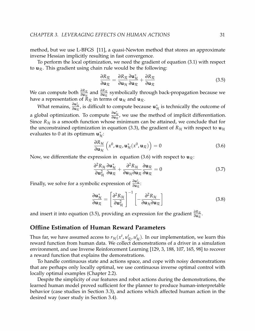
Thus far, we have assumed access to rH(xt, utR, ut
H). In our implementation, we learn thisreward function from human data. We collect demonstrations of a driver in a simulationenvironment, and use Inverse Reinforcement Learning [129, 3, 188, 107, 165, 98] to recovera reward function that explains the demonstrations.
To handle continuous state and actions space, and cope with noisy demonstrationsthat are perhaps only locally optimal, we use continuous inverse optimal control withlocally optimal examples (Chapter 2.2).
Despite the simplicity of our features and robot actions during the demonstrations, thelearned human model proved sufficient for the planner to produce human-interpretablebehavior (case studies in Section 3.3), and actions which affected human action in thedesired way (user study in Section 3.4).


CHAPTER 3. LEVERAGING EFFECTS ON HUMAN ACTIONS 33
In this section, we introduce 3 driving scenarios, and show the result of our plannerassuming a simulated human driver, highlighting the behavior that emerges from differentrobot reward functions. In the next section, we test the planner with real users andmeasure the effects of the robot’s plan. Figure 3.1 illustrates our three scenarios, andcontains images from the actual user study data.
Conditions for Analysis Across Scenarios
In all three scenarios, we start from an initial position of the vehicles on the road, asshown in Figure 3.1. In the control condition, we give the car a reward function similarto the learned RH, i.e., a linear combination of the features discussed in Chapter 2.2.Therefore, this reward function is to avoid collisions and have high velocity. We refer tothis as Rcontrol. In the experimental condition, we augment this reward function with aterm corresponding to a desired human action (e.g. low speed, lateral position, etc.). Werefer to this as Rcontrol + Raffect. Section 3.3 contrast the two plans for each of our threescenarios, and then show what happens when instead of explicitly giving the robot areward function designed to trigger certain effects on the human, we simply task therobot with reaching a destination as quickly as possible.
Scenario 1: Make Human Slow Down
In this highway driving setting, we demonstrate that an autonomous vehicle can plan tocause a human driver to slow down. The vehicles start at the initial conditions depictedon left in Figure 3.1 (a), in separate lanes. In the experimental condition, we augment therobot’s reward with the negative of the square of the human velocity, which encouragesthe robot to slow the human down.
Figure 3.1 (a) contrasts our two conditions. In the control condition, the human movesforward uninterrupted. In the experimental condition, however, the robot plans to move infront of the person, anticipating that this will cause the human to brake.
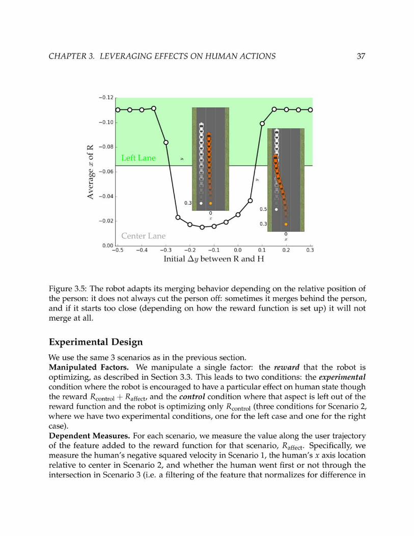
Scenario 2: Make Human Go Left/Right
In this scenario, we demonstrate that an autonomous vehicle can plan to affect thehuman’s lateral location, making the human switch lanes. The vehicles start at the initialconditions depicted on left in Figure 3.1 (b), in the same lane, with the robot ahead of thehuman. In the experimental condition, we augment the robot’s reward with the lateralposition of the human, in two ways, to encourage the robot to make the human go eitherleft (orange border image) or right (blue border image). The two reward additions areshown in Figure 3.2(a) and (b).
Figure 3.1 (b) contrasts our two conditions. In the control condition, the human movesforward, and might decide to change lanes. In the experimental condition, however, the robot
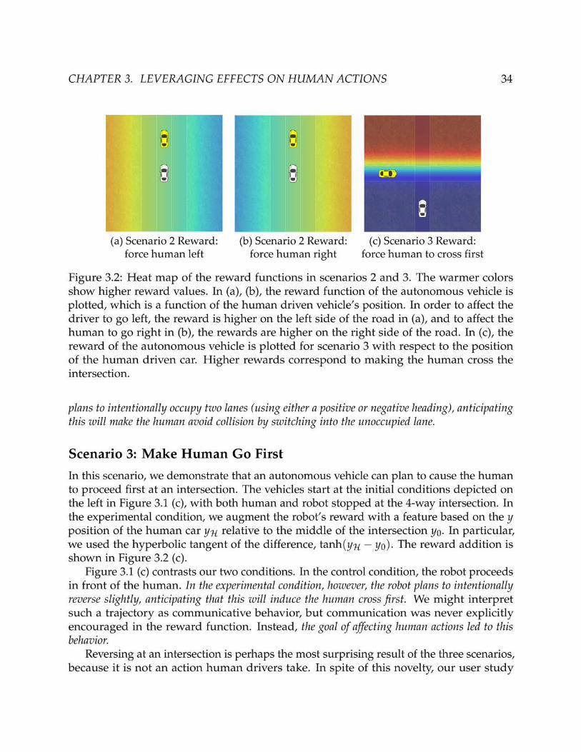


CHAPTER 3. LEVERAGING EFFECTS ON HUMAN ACTIONS 38
timing among users and measures the desired objective directly).Hypothesis. We hypothesize that our method enables the robot to achieve the effects itdesires not only in simulation, but also when interacting with real users:
The reward function that the robot is optimizing has a significant effect on the mea-sured reward during interaction. Specifically, Raffect is higher, as planned, when therobot is optimizing for it.
Subject Allocation. We recruited 10 participants (2 female, 8 male). All the participantsowned drivers license with at least 2 years of driving experience. We ran our experimentsusing a 2D driving simulator, we have developed with the driver input provided throughdriving simulator steering wheel and pedals (see Chapter 2.4).
Analysis
Scenario 1: A repeated measures ANOVA showed the square speed to be significantlylower in the experimental condition than in the control condition (F(1, 160) = 228.54,p < 0.0001). This supports our hypothesis: the human moved slower when the robotplanned to have this effect on the human.
We plot the speed and latitude profile of the human driven vehicle over time for alltrajectories in Figure 3.6. Figure 3.6(a) shows the speed profile of the control conditiontrajectories in gray, and of the experimental condition trajectories in orange. Figure 3.6(b)shows the mean and standard error for each condition. In the control condition, humansquared speed keeps increasing. In the experimental condition however, by mergingin front of the human, the robot is triggering the human to brake and reduce speed,as planned. The purple trajectory represents a simulated user that perfectly matchesthe robot’s model, showing the ideal case for the robot. The real interaction movessignificantly in the desired direction, but does not perfectly match the ideal model, sincereal users do not act exactly as the model would predict.
The figure also plots the y position of the vehicles along time, showing that the humanhas not travelled as far forward in the experimental condition.Scenario 2: A repeated measures ANOVA showed a significant effect for the rewardfactor (F(2, 227) = 55.58, p < 0.0001). A post-hoc analysis with Tukey HSD showed thatboth experimental conditions were significantly different from the control condition, withthe user car going more to the left than in the control condition when Raffect rewardsleft user positions (p < 0.0001), and more to the right in the other case (p < 0.001). Thissupports our hypothesis.
We plot all the trajectories collected from the users in Figure 3.7. Figure 3.7(a) showsthe control condition trajectories in gray, while the experimental conditions trajectoriesare shown in orange (for left) and blue (for right). By occupying two lanes, the robottriggers an avoid behavior from the users in the third lane. Here again, purple curvesshow a simulated user, i.e. the ideal case for the robot.

CHAPTER 3. LEVERAGING EFFECTS ON HUMAN ACTIONS 39
Figure 3.6: Speed profile and latitude of the human driven vehicle for Scenario 1. The firstcolumn shows the speed of all trajectories with its mean and standard errors in the bottomgraph. The second column shows the latitude of the vehicle over time; similarly, withthe mean and standard errors. The gray trajectories correspond to the control condition,and the orange trajectories correspond to the experimental condition: the robot decidesto merge in front of the users and succeeds at slowing them down. The purple plotcorresponds to a simulated user that perfectly matches the model that the robot is using.

CHAPTER 3. LEVERAGING EFFECTS ON HUMAN ACTIONS 40
Figure 3.7: Trajectories of the human driven vehicle for Scenario 2. The first column (a)shows all the trajectories, and the second column (b) shows the mean and standard error.Orange (blue) indicates conditions where the reward encouraged the robot to affect theuser to go left (right).
Scenario 3: An ordinal logistic regression with user as a random factor showed thatsignificantly more users went first in the intersection in the experimental condition thanin the baseline (χ2(1, 129) = 106.41, p < .0001). This supports our hypothesis.
Figure 3.8 plots the y position of the human driven vehicle with respect to the xposition of the autonomous vehicle. For trajectories that have a higher y position forthe human vehicle than the x position for the robot, the human car has crossed theintersection before the autonomous vehicle. The lines corresponding to these trajectoriestravel above the origin, which is shown with a blue square in this figure. The mean ofthe orange lines travel above the origin, which means that the autonomous vehicle hassuccessfully affected the humans to cross first. The gray lines travel below the origin, i.e.the human crossed second.Overall, our results suggest that the robot was able to affect the human state in the

CHAPTER 3. LEVERAGING EFFECTS ON HUMAN ACTIONS 41
Figure 3.8: Plot of yH with respect to xR. The orange curves correspond to when theautonomous vehicle affects the human to cross the intersection first. The gray curvescorrespond to the nominal setting.
desired way, even though it does not have a perfect model of the human.
3.5 Chapter Summary
In this chapter, we formalized the interaction between an autonomous (robot) vehicle anda human driver as a dynamical system, in which the actions of the robot affect those ofthe human and vice-versa. We introduced an approximate solution that enables the robotto optimize its own reward within this system. The resulting plans can purposefullymodify human behavior, and can achieve the robot’s goal more efficiently. Our user studysuggests that this is not only true in simulation, but also true when tested with real users.
Like any research, our work is limited in many ways. All this work happened in asimple driving simulator. To put this on the road, we will need more emphasis on safety,as well as a longer planning horizon. The former involves the use of formal methodsand safe control as well as better models of users: not all drivers act the same. Using aprobabilistic dynamics model as opposed to planning with the most probable humanactions, as well as estimating driving style, will be important next steps that we discuss
CHAPTER 3. LEVERAGING EFFECTS ON HUMAN ACTIONS 42
in the future chapters.An even bigger limitation is that we currently focus on a single human driver. Looking
to the interaction among multiple vehicles is not just a computational challenge, but alsoa modeling one – it is not immediately clear how to formulate the problem when multiplehuman-driven vehicles are interacting and reacting to each other. We address some ofthese limitations such as use of formal methods for safe control and estimating drivingstyle in the future chapters.
Despite these limitations, we are encouraged to see autonomous cars generate human-interpretable behaviors though optimization, without relying on hand-coded heuristics.We also look forward to applications of these ideas beyond autonomous driving, to mobilerobots, UAVs, and in general to human-robot interactive scenarios where robot actionscan influence human actions.

43
Chapter 4
Active Information Gathering overHuman Internal State
Imagine driving on the highway. Another driver is in the lane next to you, and you needto switch lanes. Some drivers are aggressive and they will never brake to let you in.Others are more defensive and would gladly make space for you. You don’t know whatkind of driver this is, so you decide to gently nudge in towards the other lane to test theirreaction. At an intersection, you might nudge in to test if the other driver is distractedand they might just let you go through (Figure 6.1 bottom left). Our goal in this chapteris to extend the optimization based approach of Chapter 3 to give robots the capability todifferentiate between human agents and plan accordingly.
In general, human behavior is affected by internal states that a robot would nothave direct access to: intentions, goals, preferences, objectives, driving style, etc. Workin robotics and perception has focused thus far on estimating these internal states byproviding algorithms with observations of humans acting, be it intent prediction [189,111, 47, 16, 17, 131], driver style prediction [102], affective state prediction [99], or activityrecognition [172].
Human state estimation has also been studied in the context of human-robot inter-action tasks. Here, the robot’s reward function depends (directly or indirectly) on thehuman internal state, e.g., on whether the robot is able to adapt to the human’s plan orpreferences. Work in assistive teleoperation or in human assistance has cast this problemas a Partially Observable Markov Decision Process, in which the robot does observe thephysical state of the world but not the human internal state — that it has to estimate fromhuman actions. Because POMDP solvers are not computationally efficient, the solutionsproposed thus far use the current estimate of the internal state to plan (either using themost likely estimate, or the entire current belief), and adjust this estimate at every step[81, 58, 18]. Although efficient, these approximations sacrifice an important aspect ofPOMDPs: the ability to actively gather information.
Our key insight is that robots can leverage their own actions to estimate the human


CHAPTER 4. ACTIVE INFORMATION GATHERING 45
Application to Driver Style Estimation. We apply our algorithm to estimating a humandriver’s style during the interaction of an autonomous vehicle with a human-drivenvehicle. Results in simulation as well as from a user study suggest that our algorithm’sability to leverage robot actions for estimation leads to significantly higher accuracy inidentifying the correct human internal state. The autonomous car plans actions likeinching forward at an intersection (Figure 6.1), nudging into another car’s lane, orbraking slightly in front of a human-driven car, all to estimate whether the human driveris attentive.
4.1 Extension to Online Estimation of the Human Model
In Chapter 3, we described the incomplete information two-player game model of theinteraction between the human and robot, and in our approximate solution, we treatedthe human’s reward function as estimated once, offline. This has worked well in our userstudy on seeking specific coordination effects on the human, like slowing down or goingfirst through the intersection. But in general, this is bound to run into problems, becausenot all people behave according to the same estimated θH.
Different drivers have different driving styles. Some are very defensive, more so thanour learned model. Others are much more aggressive, and for instance would not actuallybrake when the car merges in front of them. Even for the same driver, their style mightchange over time, for instance when they get distracted on their phone.
In this chapter, we relax our assumption of an offline estimation of the human’s rewardparameters θH. Instead, we explore estimating this online. We introduce an algorithmwhich maintains a belief over a space of candidate reward functions, and enable the robotto perform inference over this space throughout the interaction. We maintain tractabilityby clustering possible θHs into a few options that the robot maintains a belief over.
A POMDP with Human Reward as the Hidden Variable
The human’s actions are influenced by their internal reward parameters θH that the robotdoes not directly observe. So far, we estimated θH offline and solved an underactuatedsystem, a special case of an MDP. Now, we want to be able to adapt our estimate of θHonline, during interaction. This turns the problem into a partially observable Markovdecision process (POMDP) with θH as the hidden state. By putting θH in the state, wenow have a known dynamics model like in the underactuated system before for the robotand the human state, and we assume θH to remain fixed regardless of the robot’s actions.
If we could solve the POMDP, the robot would estimate θH from the human’s actions,optimally trading off between exploiting it’s current belief over θH and actively takinginformation gathering actions intended to cause human reactions, which result in a betterestimate of θH.
CHAPTER 4. ACTIVE INFORMATION GATHERING 46
Because POMDPs cannot be solved tractably, several approximations have beenproposed for similar problem formulations [81, 102, 58]. These approximations arepassively estimating the human internal state, and exploiting the belief to plan robotactions.1
In this work, we take the opposite approach: we focus explicitly on active informationgathering Our formulation enables the robot to choose to actively probe the human,and thereby improve its estimate of θH. We leverage this method in conjunction withexploitation methods, but the algorithm we present may also be used alone if humaninternal state (reward parameters) estimation is the robot’s primary objective.
Simplification to Information Gathering
We denote a belief in the value of the hidden variable, θ, as a distribution b(θ), and updatethis distribution according to the likelihood of observing a particular human action, giventhe state of the world and the human internal state:
bt+1(θ) ∝ bt(θ) · P(utH | xt, uR, θ). (4.1)
In order to update the belief b, we require an observation model. Similar to before,we assume that actions with lower reward are exponentially less likely, building on theprinciple of maximum entropy [188]:
P(uH | x, uR, θ) ∝ exp(
RθH(x0, uR, uH)
)
. (4.2)
To make explicit our emphasis on taking actions which effectively estimate θ, we rede-fine the robot’s reward function to include an information gain term, i.e., the differencebetween entropies of the current and updated beliefs: H(bt)− H(bt+1). The entropy overthe belief H(b) evaluates to:
H(b) = −∑θ b(θ) log(b(θ))
∑θ b(θ). (4.3)
We now optimize our expected reward with respect to the hidden state θ, and thisoptimization explicitly entails reasoning about the effects that the robot actions will haveon the observations, i.e., the actions that the human will take in response, and how usefulthese observations will be in shattering ambiguity about θ.
Explore-Exploit Trade-Off
In practice, we use information gathering in conjunction with exploitation. We do notsolely optimize the information gain term H(bt)− H(bt+1), but optimize it in conjunctionwith the robot’s actual reward function assuming the current estimate of θ:
1One exception is Nikolaidis et al. [132], who propose to solve the full POMDP, albeit for discrete andnot continuous state and action spaces.

CHAPTER 4. ACTIVE INFORMATION GATHERING 47
raugmentedR (xt, uR, uH) = λ(H(bt)− H(bt+1))
+ rR(xt, uR, uH, bt) (4.4)
At the very least, we do this as a measure of safety, e.g., we want an autonomous carto keep avoiding collisions even when it is actively probing a human driver to test theirreactions. We choose λ experimentally, though existing techniques that can better adaptλ over time [173].
Solution via Model Predictive Control
To find the control inputs for the robot we locally solve:
u∗R = arg maxuR
Eθ
[
RR(
x0, uR, u∗,θH (x0, uR))]
(4.5)
over a finite horizon N, where u∗,θH (x0, uR) corresponds to the actions the human would
take from state x0 if the robot executed actions uR. This objective generalizes equation (3.4)with an expectation over the current belief over θ, b0.
We still assume that the human maximizes their own reward function, rθH(xt, ut
R, utH);
we add the superscript θ to indicate the dependence on the hidden state. We can writethe sum of human rewards over horizon N as:
RθH(x0, uR, uH) =
N−1
∑t=0
rθH(xt, ut
R, utH) (4.6)
Computing this over the continuous space of possible reward parameters θ is in-tractable even with discretization. Instead, we learn clusters of θs offline via IRL, andonline use estimation to figure out which cluster best matches the human.
Despite optimizing the trade-off in equation (4.4), we do not claim that our methodas-is can better solve the general POMDP formulation: only that it can be used to getbetter estimates of human internal state. Different tradeoffs λ will result in differentperformance. Our results below emphasize the utility of gathering information, but alsotouch on the implications for active information gathering on RR.
4.2 Case Studies with Online Estimation
In this section, we show simulation results that use the method from this chapter toestimate human driver type in the interaction between an autonomous vehicle and ahuman-driven vehicle. We consider three different autonomous driving scenarios. In thesescenarios, the human is either distracted or attentive during different driving experiments.
CHAPTER 4. ACTIVE INFORMATION GATHERING 48
The scenarios are shown in Figure 6.3, where the yellow car is the autonomous vehicle,and the white car is the human driven vehicle. Our goal is to plan to actively estimate thehuman’s driving style in each one of these scenarios, by using the robot’s actions.
Attentive vs. Distracted Human Driver Models
Our technique requires reward functions rθH that model the human behavior for a partic-
ular internal state θ. We obtain a generic driver model via continuous inverse optimalcontrol with locally optimal examples [107] from demonstrated trajectories in a drivingsimulator in an environment with multiple autonomous cars, which followed precom-puted routes, similar to the previous chapter and as described in Chapter 2.2.
We then adjust the learned weights to model attentive vs. distractive drivers. Specifi-cally, we modify the weights of the collision avoidance features, so the distracted humanmodel has less weight for these features. Therefore, the distracted driver is more likely tocollide with the other cars while the attentive driver has high weights for the collisionavoidance feature. In future work, we plan to investigate ways of automatically clusteringlearned θHs from data from different users, but we show promising results even withthese simple options.
Manipulated Factors
We manipulate the reward function that the robot is optimizing. In the passive condition,the robot optimizes a simple reward function for collision avoidance based on the currentbelief estimate. It then updates this belief passively, by observing the outcomes of itsactions at every time step. In the active condition, the robot trades off between thisreward function and information gain in order to explore the human’s driving style.
We also manipulate the human internal reward parameters to be attentive or distracted.The human is simulated to follow the ideal model of reward maximization for our tworewards.
Scenarios and Qualitative Results
Scenario 1: Nudging In to Explore on a Highway. In this scenario, we show an au-tonomous vehicle actively exploring the human’s driving style in a highway drivingsetting. We contrast the two conditions in Figure 6.3(a). In the passive condition, theautonomous car drives on its own lane without interfering with the human throughoutthe experiment, and updates its belief based on passive observations gathered from thehuman car. However, in the active condition, the autonomous car actively probes the humanby nudging into her lane in order to infer her driving style. An attentive human significantlyslows down (timid driver) or speeds up (aggressive driver) to avoid the vehicle, while a distracteddriver might not realize the autonomous actions and maintain their velocity, getting closer to the


CHAPTER 4. ACTIVE INFORMATION GATHERING 50
!"#$%&'()*)#
+,--$%&'()*)#
!##&.#$%&'/01,. 2$-#3,"#&4'/01,.
(&,5'6-&3'7-)5$4'5$.&8
94&,5'6-&3':)4&5'74)##&4'5$.&8
(&,5'6-&3'7-)5$4'5$.&8
94&,5'6-&3':)4&5'74)##&4'5$.&8
(&,5'6-&3'7-)5$4'5$.&8
94&,5'6-&3':)4&5'74)##&4'5$.&8
(&,5'6-&3'7-)5$4'5$.&8
94&,5'6-&3':)4&5'74)##&4'5$.&8
Figure 4.3: Legends indicating active/passive robots, attentive/distracted humans, andreal user/ideal model used for all following figures.
Quantitative Results
Throughout the remainder of this chapter, we use a common color scheme to plot resultsfor our experimental conditions. We show this common scheme in Figure 4.3: darkercolors (black and red) correspond to attentive humans, and lighter colors (gray andorange) correspond to distracted humans. Further, the shades of orange correspondto active information gathering, while the shades of gray indicate passive informationgathering. We also use solid lines for real users, and dotted lines for scenarios with anideal user model learned through inverse reinforcement learning.
Figure 4.4 plots, using dotted lines, the beliefs over time for the attentive (left) anddistracted (right) conditions, comparing in each the passive (dotted black and grayrespectively) with the active method (dotted dark orange and light orange respectively).In every situation, the active method achieves a more accurate belief (higher values forattentive on the left, when the true θ is attentive, and lower values on the right, when thetrue θ is distracted). In fact, passive estimation sometimes incorrectly classifies drivers asattentive when they are distracted and vice-versa.
The same figure also shows (in solid lines) results from our user study of whathappens when the robot no longer interacts with an ideal model. We discuss these in thenext section.
Figure 4.5 and Figure 5.6 plot the corresponding robot and human trajectories for eachscenario. The important takeaway from these figures is that there tends to be a largergap between attentive and distracted human trajectories in the active condition (orangeshades) than in the passive condition (gray shades), especially in scenarios 2 and 3. Itis this difference that helps the robot better estimate θ: the robot in the active condition ispurposefully choosing actions that will lead to large differences in human reactions, in order tomore easily determine the human driving style.

CHAPTER 4. ACTIVE INFORMATION GATHERING 51
Figure 4.4: The probability that the robot assigns to attentive as a function of time, forthe attentive (left) and distracted (right). Each plot compares the active algorithm topassive estimation, showing that active information gathering leads to more accuratestate estimation, in simulation and with real users.


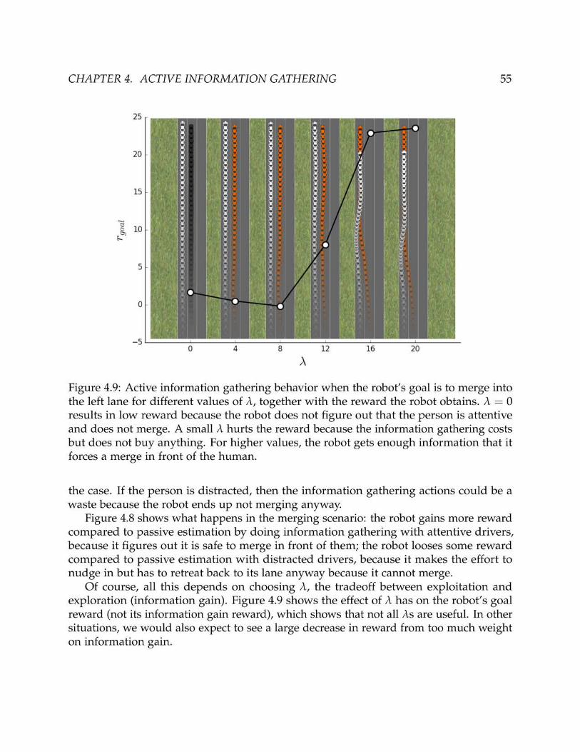

CHAPTER 4. ACTIVE INFORMATION GATHERING 56
Beyond Driving Style: Active Intent Inference
Driving style is not the only type of human internal state that our method enables robotsto estimate. If the human has a goal, e.g. of merging into the next lane or not, or of exitingthe highway or not, the robot could estimate this as well using the same technique.
Each possible goal corresponds to a feature. When estimating which goal the humanhas, the robot is deciding among θs which place weight on only one of the possiblegoal features, and 0 on the others. Figure 4.10 shows the behavior that emerges fromestimating whether the human wants to merge into the robot’s lane. In the passive case,the human is side by side with the robot. Depending on the driving style, they mightslow down slightly, accelerate slightly, or start nudging into the robot’s lane, but sincethe observation model is noisy the robot does not get quite enough confidence in thehuman’s intent early on. Depending on the robot’s reward, it might take a long timebefore the person can merge. In the active case, the robot decides to probe the person byslowing down and shifting away from the person in order to make room. It then becomesoptimal for the person wanting to merge to start shifting towards the robot’s lane, givingthe robot enough information now to update its belief. In our experiment, we see thatthis is enough for the person to be able to complete the merge faster, despite the robotnot having any incentive to help the person in its reward.
4.3 User Study with Online Estimation
In the previous section, we explored planning for an autonomous vehicle that activelyprobes a human’s driving style, by braking or nudging in and expecting to cause reactionsfrom the human driver that would be different depending on their style. We showedthat active exploration does significantly better at distinguishing between attentive anddistracted drivers using simulated (ideal) models of drivers. Here, we show the resultsof a user study that evaluates this active exploration for attentive and distracted humandrivers.
Experimental Design
We use the same three scenarios discussed in the previous section.Manipulated Factors. We manipulated the same two factors as in our simulation experi-ments: the reward function that the robot is optimizing (whether it is optimizing its rewardthrough passive state estimation, or whether it is trading off with active informationgathering), and the human internal state (whether the user is attentive or distracted). Weasked our users to pay attention to the road and avoid collisions for the attentive case,and asked our users to play a game on a mobile phone during the distracted drivingexperiments.Dependent Measure. We measured the probability that the robot assigned along the wayto the human internal state.


CHAPTER 4. ACTIVE INFORMATION GATHERING 58
Hypothesis. The active condition will lead to more accurate human internal state estimation,regardless of the true human internal state.Subject Allocation. We recruited 8 participants (2 female, 6 male) in the age range of21-26 years old. All participants owned a valid driver license and had at least 2 yearsof driving experience. We ran the experiments using a 2D driving simulator with thesteering input and acceleration input provided through a steering wheel and a pedals asshown in Figure 6.1 and described in Chapter 2.4. We used a within-subject experimentdesign with counterbalanced ordering of the four conditions.
Analysis
We ran a factorial repeated-measures ANOVA on the probability assigned to “attentive”,using reward (active vs passive) and human internal state (attentive vs distracted) asfactors, and time and scenario as covariates. As a manipulation check, attentive drivershad significantly higher estimated probability of “attentive” associated than distracteddrivers (.66 vs .34, F = 3080.3, p < .0001). More importantly, there was a signifiantinteraction effect between the factors (F = 1444.8, p < .000). We ran a post-hoc analysiswith Tukey HSD corrections for multiple comparisons, which showed all four conditionsto be significantly different from each other, all contrasts with p < .0001. In particular,the active information gathering did end up with higher probability mass on “attentive”than the passive estimation for the attentive users, and lower probability mass forthe distracted user. This supports our hypothesis that our method works, and activeinformation gathering is better at identifying the correct state.
Figure 4.4 compares passive (grays and blacks) and active (light and dark oranges)across scenarios and for attentive (left) and distracted (right) users. It plots the probabilityof attentive over time, and the shaded regions correspond to standard error. From thefirst column, we can see that our algorithm in all cases detects human’s attentiveness withmuch higher probably than the passive information gathering technique shown in black.From the second column, we see that our algorithm places significantly lower probabilityon attentiveness, which is correct because those users were distracted users. These arein line with the statistical analysis, with active information gathering doing a better jobestimating the true human internal state.
Figure 4.5 plots the robot trajectories for the active information gathering setting.Similar to Figure 4.4, the solid lines are the mean of robot trajectories and the shadedregions show the standard error. We plot a representative dimension of the robot trajectory(like position or speed) for attentive (dark orange) or distracted (light orange) cases. Theactive robot probed the user, but ended up taking different actions when the user wasattentive vs. distracted in order to maintain safety. For example, in Scenario 1, thetrajectories show the robot is nudging into the human’s lane, but the robot decides tomove back to its own lane when the human drivers are distracted (light orange) in orderto stay safe. In Scenario 2, the robot brakes in front of the human, but it brakes less when

CHAPTER 4. ACTIVE INFORMATION GATHERING 59
the human is distracted. Finally, in Scenario 3, the robot inches forward, but again itstops when if the human is distracted, and even backs up to make space for her.
Figure 5.6 plots the user trajectories for both active information gathering (first row)and passive information gathering (second row) conditions. We compare the reactions ofdistracted (light shades) and attentive (dark shades) users. There are large differencesdirectly observable, with user reactions tending to indeed cluster according to theirinternal state. These differences are much smaller in the passive case (second row, wheredistracted is light gray and attentive is black). For example, in Scenario 1 and 2, theattentive users (dark orange) keep a larger distance to the car that nudges in front ofthem or brakes in front of them, while the distracted drivers (light orange) tend to keep asmaller distance. In Scenario 3, the attentive drivers tend to slow down and do not crossthe intersection, when the robot actively inches forward. None of these behaviors can bedetected clearly in the passive information gathering case (second row). This is the coreadvantage of active information gathering: the actions are purposefully selected by therobot such that users would behave drastically differently depending on their internalstate, clarifying to the robot what this state actually is.Overall, these results support our simulation findings, that our algorithm performsbetter at estimating the true human internal state by leveraging purposeful informationgathering actions.
4.4 Chapter Summary
In this chapter, we took a step towards autonomously producing behavior for interactionand coordination between autonomous cars and human-driven vehicles. We introducedan online estimation algorithm in which the robot actively uses its actions to gatherinformation about the human model so that it can better plan its own actions. Ouranalysis again shows coordination strategies arising out of planning in our formulation:the robot nudges into someones’s lane to check if the human is paying attention, andonly completes the merge if they are; the robot inches forward at an intersection, again tocheck if the human is paying attention, and proceeds if they are, but backs up to let themthrough if they are not; the robot slows down slightly and shifts in its lane away from thehuman driver to check if they want to merge into its lane or not.
Importantly, these behaviors change with the human driver style and with the initialconditions – the robot takes different actions in different situations, emphasizing the needto start generating such coordination behavior autonomously rather than relying on handcoded strategies. Even more importantly, the behaviors seem to work when the robot isplanning and interacting with real users.Limitations. While performing our experiments, we found the robot’s nominal rewardfunction (trading off between safety and reaching a goal) to be insufficient – in somecases it led to getting dangerously close to the human vehicle and even collisions, goingoff the road, oscillating in the lane due to minor asymmetries in the environment, etc.
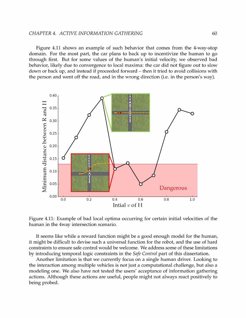

CHAPTER 4. ACTIVE INFORMATION GATHERING 61
Conclusion. We are encouraged by the fact that robots can generate useful behavior forinteraction autonomously, and plan to explore information-gathering actions on humanstate further, including beyond autonomous driving scenarios.

62
Chapter 5
Active Preference-Based Learning ofReward Functions
Reward functions play a central role in specifying how dynamical systems should act: howan end-user wants their assistive robot arm to move, or how they want their autonomouscar to drive. For many systems, end-users have difficulty providing demonstrations ofwhat they want. For instance, they cannot coordinate 7 degrees of freedom (DOFs) at atime [6], and they can only show the car how they drive, not how they want the car todrive [20]. In such cases, another option is for the system to regress a reward functionfrom labeled state-action pairs, but assigning precise numeric reward values to observedrobot actions is also difficult.
In this chapter, we propose a preference-based approach to learning desired rewardfunctions in a dynamical system. Instead of asking for demonstrations, or for the value ofthe reward function for a sample trajectory (e.g., “rate the safety of this driving maneuverfrom 1 to 10”), we ask people for their relative preference between two sample trajectories(e.g., “is ξ1 more safe or less safe than ξ2?”).
Active preference-based learning has been successfully used in many domains [4, 90,33, 32], but what makes applying it to learning reward functions difficult is the complexityof the queries, as well as the continuous nature of the underlying hypothesis space ofpossible reward functions. We focus on dynamical systems with continuous or hybriddiscrete-continuous state. In this setting, queries consist of two candidate continuousstate and action space trajectories that satisfy the system’s dynamics, in an environmentor scenario that the learning algorithm also needs to decide on, consisting of an initialstate and the trajectories of other agents in the scene. Consider again the example ofautonomous driving. In this situation, a query would consist of two trajectories for thecar from some starting state among other cars following their own trajectories.
Typically in preference-based learning, the queries are actively selected by searchingsome discrete or sampled set (e.g., [78, 80, 63, 180, 167, 7]). Our first hypothesis is that inour setting, the continuous and high-dimensional nature of the queries renders relyingon a discrete set ineffective. Preference-based work for such spaces has thus far collected
CHAPTER 5. ACTIVE PREFERENCE-BASED LEARNING 63
data passively [181, 151]. Our second hypothesis is that active generation of queries leadsto better reward functions faster.
We contribute an algorithm for actively synthesizing queries from scratch. We docontinuous optimization in query space to maximize the expected volume removed fromthe hypothesis space. We use the human’s response to assign weights to the hypothesisspace in the form of a log-concave distribution, which provides an approximation ofthe objective via a Metropolis algorithm that makes it differentiable w.r.t. the queryparameters. We provide a bound on the number of iterations required to converge.
We compare our algorithm to non-active and non-synthesis approaches to test ourhypotheses. We use an experimental setup motivated by autonomous driving, and showthat our approach converges faster to a desired reward function. Finally, we illustratethe performance of our algorithm in terms of accuracy of the reward function learnedthrough an in-lab usability study.
5.1 Preference-Based Learning Problem
Modeling Choices
Our goal is to model the behavior and preferences of a human H for how a dynamicalsystem should act. Similar to the previous chapters (as discussed in Chapter 2), we modelthe overall system including H, and all the other agents (robot R) as a fully-observabledynamical system.
We define a trajectory ξ ∈ Ξ, where ξ = (x0, u0R, u0
H), . . . , (xN, uNR , uN
H) is a finitehorizon sequence of states and actions of all agents. Here, Ξ is a set of all feasiblecontinuous trajectories. A feasible trajectory is one that satisfies the dynamics of H andR. As in IRL (see Chapter 2.2), we parameterize the preference reward function as alinear combination of a set of features:
rH(xt, utR, ut
H) = w⊤φ(xt, utR, ut
H), (5.1)
with w being a vector of the weights for the feature function φ(xt, utR, ut
H) evaluated at ev-ery state and action pair. We assume a d-dimensional feature function, so φ(xt, ut
R, utH) ∈
Rd.For simpler notation, we combine the N + 1 elements of φ so Φ = ∑
Nt=0 φ(xt, ut
R, utH).
Therefore, Φ(ξ) evaluates over a trajectory ξ. We finally reformulate the reward functionas the following inner product:
RH(ξ) = w ·Φ(ξ). (5.2)
Our goal is to learn RH.
CHAPTER 5. ACTIVE PREFERENCE-BASED LEARNING 64
Approach Overview
Inverse Reinforcement Learning (IRL) [188, 107, 159] enables us to learn RH throughdemonstrated trajectories. However, IRL requires the human to show demonstrationsof the optimal sequence of actions. Providing demonstrations can be challenging formany human-robot tasks. Furthermore, generating interesting training data that activelyexplores RH through atypical, interesting environments (which is necessary in manycases for resolving ambiguities) works well [116, 41] but in practice can make (good)demonstrations infeasible: the algorithm cannot physically manufacture environments,and therefore relies on simulation, which makes demonstrations only possible throughteleoperation.
For these reasons, we assume demonstrations are not available in this chapter. Instead,we propose to leverage preference-based learning, which queries H to provide compar-isons between two candidate trajectories. We propose a new approach for active learningof a reward function for human preferences through comparisons.
We split trajectories ξ into two parts: a scenario and the trajectory of the agentH whose reward function we are learning. We formalize a scenario to be the initialstate of the environment as well as the sequence of actions for the other agent(s) R,τ = (x0, u0
R, . . . , uNR). Given an environment specified by scenario τ ∈ T , the human
agent will provide a finite sequence of actions uH = u0H, . . . , uN
H in response to scenario τ.This response, along with the scenario τ defines a trajectory ξ showing the evolution ofthe two systems together in the environment.
We iteratively synthesize queries where we ask the human to compare between twotrajectories ξA and ξB defined over the same fixed scenario τ as shown in Figure 5.1(a). Their answer provides us information about w. In what follows, we discuss howto update our probability distribution over w given the answer to a query, and how toactively synthesize queries in order to efficiently converge to the right w.
5.2 Learning Reward Weights from Preferences of
Synthesized Queries
In this section, we describe how we update a distribution over reward parameters (weightsw in equation (5.2)) based on the answer of one query. We first assume that we are atiteration t of the algorithm and an already synthesized pair of trajectories ξA and ξB in acommon scenario is given (we discuss in the next section how to generate such a query).We also assume H has provided her preference for this specific pair of trajectories atiteration t. Let her answer be I, with It = +1 if she prefers the former, and It = −1 ifshe prefers the latter. This answer gives us information about w: she is more likely tosay +1 if ξA has higher reward than ξB, and vice-versa, but she might not be exact indetermining It. We thus model the probability p(I|w) as noisily capturing the preference

CHAPTER 5. ACTIVE PREFERENCE-BASED LEARNING 65
w.r.t. RH:
p(It|w) =
exp(RH(ξA))exp(RH(ξA))+exp(RH(ξB))
It = +1
exp(RH(ξB))exp(RH(ξA))+exp(RH(ξB))
It = −1
(5.3)
We start with a prior over the space of all w, i.e., w is uniformly distributed on theunit ball. Note that the scale of w does not change the preference It, so we can constrain||w|| ≤ 1 to lie in this unit ball. After receiving the input of the human It, we proposeusing a Bayesian update to find the new distribution of w:
p(w|It) ∝ p(w) · p(It|w). (5.4)
Letϕ = Φ(ξA)−Φ(ξB) (5.5)
Then our update function that multiplies the current distribution at every step is:
fϕ(w) = p(It|w) =1
1 + exp(−Itw⊤ϕ)(5.6)
Updating the distribution of w allows us to reduce the probability of the undesiredparts of the space of w, and maintain the current probability of the preferred regions.
5.3 Synthesizing Queries through Active Volume
Removal
The previous section showed how to update the distribution over w after getting theresponse to a query. Here, we show how to synthesize the query in the first place: wewant to find the next query such that it will help us remove as much volume (the integralof the unnormalized pdf over w) as possible from the space of possible rewards.
Formulating Query Selection as Constrained Optimization
We synthesize experiments by maximizing the volume removed under the feasibilityconstraints of ϕ:
maxϕ
minE[1− fϕ(w)], E[1− f−ϕ(w)]
subject to ϕ ∈ F(5.7)
The constraint in this optimization requires ϕ to be in the feasible set F:
F = ϕ : ϕ = Φ(ξA)−Φ(ξB), ξA, ξB ∈ Ξ,
τ = (x0, uAR) = (x0, uB
R)(5.8)


CHAPTER 5. ACTIVE PREFERENCE-BASED LEARNING 67
p(w) by the empirical distribution composed of point masses at wi’s:
p(w) ∼ 1
M
M
∑i=1
δ(wi). (5.10)
Then the volume removed by an update fϕ(w) can be approximated by:
E[1− fϕ(w)] ≃ 1
M
M
∑i=1
(1− fϕ(wi)). (5.11)
Given such samples, the objective is now differentiable w.r.t. ϕ, which is differentiablew.r.t. the starting state and controls – the ingredients of the query which are the variablesin equation (10.2). What remains is to get the actual samples. To do so, we take advantageof the fact that p(w) is a log-concave function, and the update function fϕ(w) defined hereis also log-concave in w as shown in Figure 5.1 (c); therefore, the posterior distributionof w stays log-concave. Note we do not need to renormalize the distribution p(w) aftera Bayesian update, i.e. divide p(w) by its integral. Instead, we use Metropolis MarkovChain methods to sample from p(w) without normalization.
Log-concavity is useful because we can take advantage of efficient polynomial timealgorithms for sampling from the current p(w) [117]1. In practice, we use an adaptiveMetropolis algorithm, where we initialize with a warm start by computing the mode ofthe distribution, and perform a Markov walk [74].
We could find the mode of fϕ from (5.6), but it requires a convex optimization. Weinstead speed this up by choosing a similar log-concave function whose mode evaluates tozero always, and which reduces the probability of undesired w by a factor of exp(Itw
⊤ϕ):
fϕ(w) = min(1, exp(Itw⊤ϕ)) (5.12)
Figure 5.1 (c) shows this simpler choice of update function in black with respect to p(It|w)in gray. The shape is similar, but enables us to start from zero, and a Markov walk willefficiently sample from the space of w.
In Figure 5.1 (b), we show a simple diagram demonstrating our approach. Here,w first uniformly lies on a unit d-dimensional ball. For simplicity, here we show a 3Dball. The result of a query at every step is a state and trajectories that result in a featuredifference vector ϕ, normal to the hyperplane w : w⊤ϕ = 0, whose direction representsthe preference of the human, and its value lies in F defined in equation (5.8). We reducethe volume of w by reducing the probability distribution of the samples of w on therejected side of the hyperplane through the update function fϕ(w) that takes into accountnoise in the comparison.
1Note that computing the actual volume removed can be converted to the task of integrating a log-concave function, for which efficient algorithms do exist. The purpose of using samples instead is to havean expression suitable for maximization of volume removed, i.e. an expression differentiable w.r.t. thequery.

CHAPTER 5. ACTIVE PREFERENCE-BASED LEARNING 68
5.4 Algorithm and Performance Guarantees
Armed with a way of generating queries and a way of updating the reward distributionbased on the human’s answer to each query, we now present our method for activelylearning a reward function in Algorithm 1. The inputs to the algorithm are a set offeatures φ, the desired horizon N, the dynamics of the system f , and the number ofiterations iter. The goal is to converge to the true distribution of w, which is equivalent tofinding the preference reward function RH(ξ) = w ·Φ(ξ).
We first initialize this distribution to be uniform over a unit ball in line 3. Then, for Miterations, the algorithm repeats these steps: volume estimation, synthesizing a feasiblequery, querying the human, and updating the distribution.
We sample the space of w in line 5. Using these samples, and the dynamics of thesystem, SynthExps solves the optimization in equation (10.2): it synthesizes a feasiblepair of trajectory that maximizes the expected volume removed from the distribution ofp(w). The answer to the query is received in line 7. We compute fϕ(w), and update thedistribution in line 10.
Algorithm 1 Preference-Based Learning of Reward Functions
1: Input: Features φ, horizon N, dynamics f , iter2: Output: Distribution of w: p(w)3: Initialize p(w) ∼ Uniform(B), for a unit ball B4: While t < iter:5: W ← M samples from AdaptiveMetropolis(p(w))6: (x0, uR, uA
H, uBH)← SynthExps(W, f )
7: It ← QueryHuman(x0, uR, uAH, uB
H)8: ϕ = Φ(x0, uR, uA
H)−Φ(x0, uR, uBH)
9: fϕ(w) = min(1, It exp(w⊤ϕ))10: p(w)← p(w) · fϕ(w)11: t← t + 112: End for
Regarding the convergence of Algorithm 1, one cannot generally make any strictclaims for several reasons: We replace the distribution p(w) by an empirical distribution,which could introduce errors. The maximization in line 6 is via non-convex optimizationwhich does not necessarily find the optimum, and even if it was guaranteed that theglobal optimum is found, it could potentially make very little progress in terms of volumeremoval, since the set F can be arbitrary.
Putting aside the issues of sampling and global optimization, we can compare whatAlgorithm 1 does to the best one could do with the set F. Algorithm 1 can be thought ofas a greedy volume removal.
Theorem 1. Under the following assumptions:

CHAPTER 5. ACTIVE PREFERENCE-BASED LEARNING 69
• The update function is fϕ as defined in equation (5.6),
• The human inputs are noisy similar to equation (5.3),
• The errors introduced by sampling and non-convex optimization are ignored,
Algorithm 1 removes at least 1− ǫ times as much volume as removed by the best adaptive strategyafter ln(1
ǫ ) times as many iterations.
Proof. Removed volume can be seen to be an adaptive submodular function, defined interms of the choices ϕ and the human input It, as defined in [69]. It is also adaptivemonotone; thus, the results of [69] imply that greedy volume removal for l steps inexpectation removes at least (1− exp(−l/k))OPTk where OPTk is the best solution anyadaptive strategy can achieve after k steps. Setting l = k ln(1
ǫ ) gives us the desired result.One caveat is that in equation (5.6) the human input It is treated as worst case, i.e., in
the synthesis step, one maximizes the minimum removed volume (over the possible It).Namely maximizing the following quantity:
minEw[1− Pr[It = +1|w]]), Ew[1− Pr[It = −1|w]]). (5.13)
Normally the greedy strategy in adaptive submodular maximization should treat It asprobabilistic. In other words instead of the minimum one should typically maximize thefollowing quantity:
Pr[It = +1] ·Ew[1− Pr[It = +1|w]]+
Pr[It = −1] ·Ew[1− Pr[It = −1|w]].(5.14)
However, note Ew[1− Pr[It = +1|w]] is simply Pr[It = −1] and similarly Ew[1−Pr[It = +1|w]] is Pr[It = +1]. Therefore, Algorithm 1 is maximizing min(Pr[It =−1], Pr[It = +1]), whereas greedy submodular maximization should be maximizing2 Pr[It = −1]Pr[It = +1]. It is easy to see that these two maximizations are equivalent,since the sum Pr[It = −1] + Pr[It = +1] = 1 is fixed.
5.5 Simulation Experiment
In this section, we evaluate our theory using a semiautonomous driving example. Ourgoal is to learn people’s preferred reward function for driving. In this context, ourapproach being preference-based is useful since it allows the users to only compare twocandidate trajectories in various scenarios instead of requiring the user to demonstrate afull trajectory (of how they would like to drive, not how they actually drive). In addition,our approach being active enables choosing informative test cases that are otherwisedifficult to encounter in driving scenarios. For example, we can address the preferenceof drivers in moral dilemma situations (deciding between two undesirable outcomes),which are very unlikely to arise in standard collected driving data. Finally, our approach

CHAPTER 5. ACTIVE PREFERENCE-BASED LEARNING 71
synthesizes these test cases from scratch, which should help better exploit the continuousand high-dimensional space of queries. We put these advantages to the test in whatfollows.
Experimental Setup
We assume a human driven vehicle H living in an environment with another vehicleR, and we synthesize trajectories containing two candidate sequence of actions for thehuman driven car, while for every comparison we fix the synthesized scenario (i.e., theinitial state of the environment and the sequence of actions of R). Figure 5.1 (a) shows anexample of this comparison. The white vehicle isR, and the orange vehicle corresponds toH. The white and orange lines show the path taken by the human and robot, respectively,in the two cases over a horizon of N = 5.
Assuming the vehicles follow the same dynamics model as in Chapter 2.4, we learnthe reward function of the human’s preferences based on queries similar to Figure 5.1 (a).We define a set of features that allow representing this cost function. These are the samefeatures introduced in Chapter 2.2, i.e., φ1 ∝ c1 · exp(−c2 · d2) corresponds to penalizinggetting close to the boundaries of the road, where d is the distance between the vehicle andthese boundaries, and c1 and c2 are appropriate scaling factors. We use a similar featureφ2 for enforcing staying within a single lane by penalizing leaving the boundaries of thelane. We also encourage higher speed for moving forward through φ3 = (v− vmax)2,where v is the velocity of the vehicle, and vmax is the speed limit. Also, we would like thevehicle to have a heading along with the road using a feature φ4 = βH · n, where βH is theheading of H, and n is a normal vector along the road. Our last feature φ5 corresponds tocollision avoidance, and is a non-spherical Gaussian over the distance of H and R, whosemajor axis is along the robot’s heading. Then, we aim to learn a distribution over theweights corresponding to these features w =
[
w1 w2 w3 w4 w5
]
so RH = w · Φ(ξ)best represents the preference reward function.
Conditions
We compare our algorithm with two baselines: non-active and non-synthesis.First, we compare it to a non-active version. Instead of actively generating queries that
will remove the most volume, we uniformly sample a scenario. We do not use totallyrandom trajectories for the cars as this would be a weak baseline, instead we sampletwo candidate weight vectors wA and wB from the current distribution on w. We thenmaximize the reward functions wA ·Φ(ξA) and wB ·Φ(ξB) to solve for optimal uA
H and
uBH. That creates our query, comparing two reward functions, but no longer optimized to
efficiently learn w. The trajectories generated through this other approach are then usedto query the human, and update the distribution of p(w) similar to Algorithm 1. Second,we compare it against a non-synthesis (discrete) version. Instead of solving a continuous
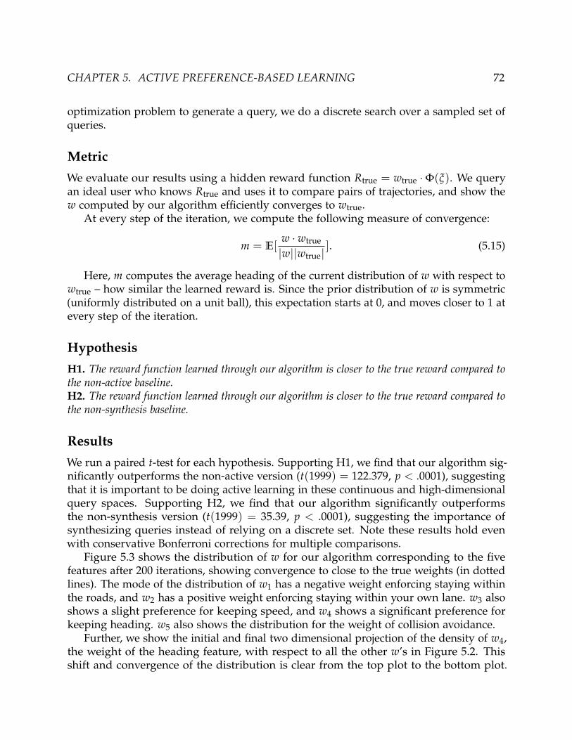
CHAPTER 5. ACTIVE PREFERENCE-BASED LEARNING 72
optimization problem to generate a query, we do a discrete search over a sampled set ofqueries.
Metric
We evaluate our results using a hidden reward function Rtrue = wtrue ·Φ(ξ). We queryan ideal user who knows Rtrue and uses it to compare pairs of trajectories, and show thew computed by our algorithm efficiently converges to wtrue.
At every step of the iteration, we compute the following measure of convergence:
m = E[w · wtrue
|w||wtrue|]. (5.15)
Here, m computes the average heading of the current distribution of w with respect towtrue – how similar the learned reward is. Since the prior distribution of w is symmetric(uniformly distributed on a unit ball), this expectation starts at 0, and moves closer to 1 atevery step of the iteration.
Hypothesis
H1. The reward function learned through our algorithm is closer to the true reward compared tothe non-active baseline.H2. The reward function learned through our algorithm is closer to the true reward compared tothe non-synthesis baseline.
Results
We run a paired t-test for each hypothesis. Supporting H1, we find that our algorithm sig-nificantly outperforms the non-active version (t(1999) = 122.379, p < .0001), suggestingthat it is important to be doing active learning in these continuous and high-dimensionalquery spaces. Supporting H2, we find that our algorithm significantly outperformsthe non-synthesis version (t(1999) = 35.39, p < .0001), suggesting the importance ofsynthesizing queries instead of relying on a discrete set. Note these results hold evenwith conservative Bonferroni corrections for multiple comparisons.
Figure 5.3 shows the distribution of w for our algorithm corresponding to the fivefeatures after 200 iterations, showing convergence to close to the true weights (in dottedlines). The mode of the distribution of w1 has a negative weight enforcing staying withinthe roads, and w2 has a positive weight enforcing staying within your own lane. w3 alsoshows a slight preference for keeping speed, and w4 shows a significant preference forkeeping heading. w5 also shows the distribution for the weight of collision avoidance.
Further, we show the initial and final two dimensional projection of the density of w4,the weight of the heading feature, with respect to all the other w’s in Figure 5.2. Thisshift and convergence of the distribution is clear from the top plot to the bottom plot.

CHAPTER 5. ACTIVE PREFERENCE-BASED LEARNING 74
of the queries (or even producing actual concrete queries), they overall perform betterthan when the algorithms need to generate real queries. In this case, being active is stillimportant, but the ability to perform synthesis is no longer useful compared to relyingon a discrete set. Without needing to produce trajectories, a discrete set covers the muchlower dimensional space of feature differences, and discrete search is not bottleneckedby local optima. This suggests that indeed, synthesis is important when we are dealingwith learning reward functions for dynamical systems, requiring queries in a continuous,high-dimensional, and dynamically constrained space.
Overall, the results suggest that doing active query synthesis is important in rewardlearning applications of preference-based learning, with our results supporting both ofour central hypotheses and demonstrating an improvement over prior methods whichare either non-active or non-synthesis.
5.6 Usability Study
Our experiments so far supported the value of our contribution: active preference-basedlearning that synthesizes queries from scratch outperformed both non-active and non-synthesis learning. Next, we ran a usability study with human subjects. The purpose ofthis study is not to compare our algorithm once again with other methods. Instead, wewanted to test whether a person can interact with our algorithm to recover a reasonablereward function for dynamical systems with continuous state and action spaces.
Experimental Design
In the learning phase of the experiments, we jumpstart the weights w with a referencestarting distribution, and only update that based on the data collected for each user. Weask for 10 query inputs to personalize the distribution of w for each user.
Unlike our simulation experiments, here we do not have access to the ground truthreward function. Still, we need to evaluate the learned reward function. We thus evaluatewhat the users think subjectively about the behavior produced on a 7 point Likert scale.
Manipulated Factors
In order to calibrate the scale, we need to compare the reward’s rating with somebaseline. We choose to perturb the learned reward for this calibration. Thus, we onlymanipulate one factor: perturbation from the learned weights. We ask users to comparetrajectories obtained by optimizing for reward with three different values for the weights:i) w∗ = E[w] providing the mode of the learned distribution from Algorithm 1, ii) w2
a large perturbation of w∗ which enables us to sanity check that the learned reward isbetter than a substantially different one, and iii) w1 a slight perturbation of w∗, which is aharder baseline to beat and enables us to test that the learned reward is a local optimum.

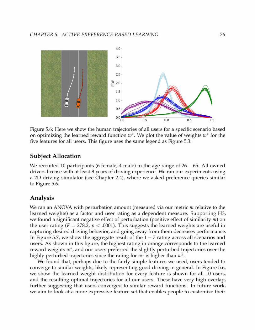


CHAPTER 5. ACTIVE PREFERENCE-BASED LEARNING 78
preference for the trajectory emerging from the learned weights, but it does not yet showthat people can use this to personalize for their behavior – most users end up with verysimilar learned weights, and we believe this is because of the limitations of our featuresand our simulator. We plan to address these in the future.

79
Chapter 6
Falsification for Human-Robot Systems
In this chapter, we discuss a new approach for a rigorous analysis of human-robotsystems that are based on learned models of human behavior. We focus on analyzing therobustness of a learning-based controller for human-robot systems where the humanbehavior deviates slightly from a learned model. As a motivating application, we considerautonomous controllers for vehicles that are based on the common and effective modelpredictive control (MPC) paradigm (see Chapter 2.1), in the receding horizon sense. Inthis setting, the autonomous controller computes its control actions for a horizon of Ntime units, while optimizing its reward function (which typically encodes safety andother objectives). For this purpose, it uses a dynamical model of both the system undercontrol and its environment. Additionally, the environment contains human agentswho are modeled as rational agents seeking to take actions that maximize their rewardfunction. However, the human’s true reward function is unknown to the autonomouscontroller. Therefore, the controller learns an approximation of the reward functionfrom collected data, and uses this learned function in computing its actions. We refer tosuch a controller as an interaction-aware controller as described in the previous chapters(Chapter 3 and Chapter 4). Our goal is to find behaviors that exhibit “bugs”, i.e., wherethe controller fails to meet its objectives. We refer to this goal as falsification.
Falsification of such human-robot systems faces some unique challenges. First, sincethe human model is learned from incomplete data, under specific assumptions and biasesof the learning algorithm, and the true reward function is unknown, the learned modelwill be inaccurate. In such a setting, how can one bound the error in the learned model?Second, given an error bound, how can one systematically verify whether the controllerwill always achieve the desired objectives in an environment where the human agent(s)deviate from the learned model within that error bound?
Our approach addresses both challenges using optimization-based algorithmic meth-ods. For the first, we provide a systematic and efficient methodology for estimatinga bound between the values of the human’s true reward function and the controller’sestimate. Our methodology generates experiments to use in human subject trials duringthe learning process. For the second challenge, we present a novel encoding of the falsifi-
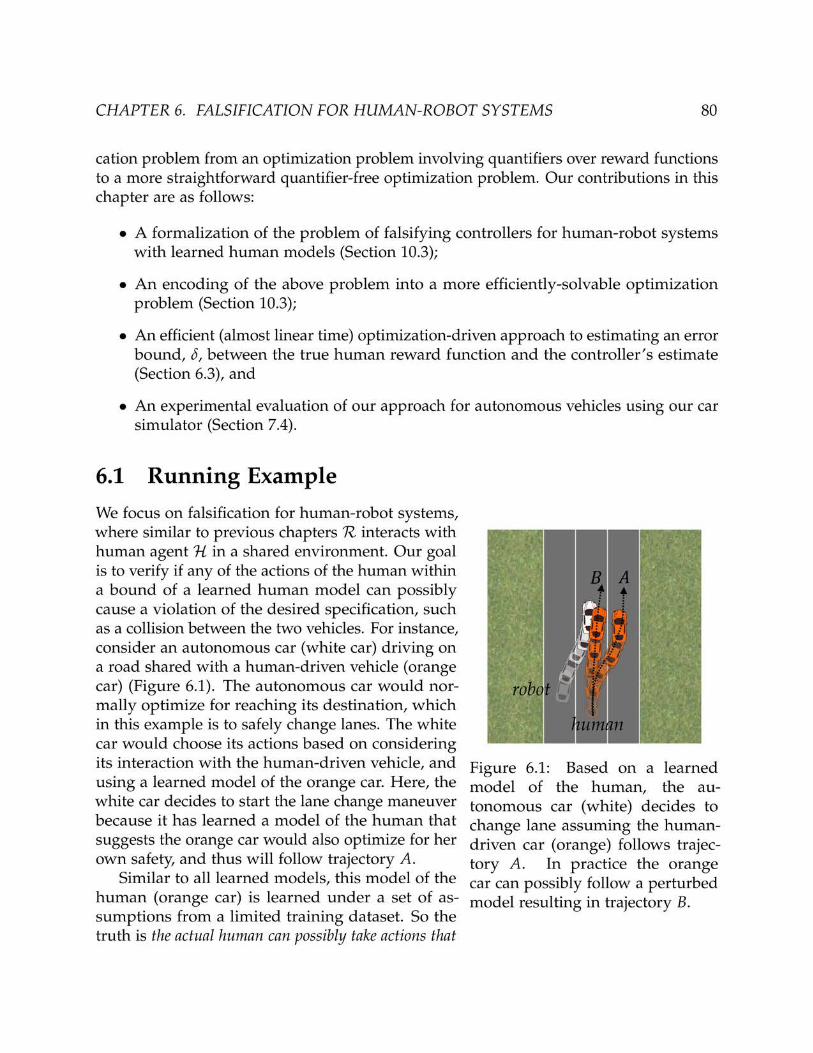

CHAPTER 6. FALSIFICATION FOR HUMAN-ROBOT SYSTEMS 81
slightly differ from the robot’s learned human model. For example, the orange car mightdecide to choose a slightly perturbed trajectory such as trajectory B. As it is clear in Fig-ure 6.1, such a perturbation can jeopardize satisfaction of the desired properties such ascollision avoidance.
In this chapter, we show that these perturbations in models of learned human driversexist, and we provide an efficient algorithm (almost linear) to learn a distribution for suchpossible perturbations using a query-based method. Further, we provide a method forfinding the falsifying actions of the human agent (e.g. actions that result in trajectory B)within the perturbation bound.
6.2 Falsification in Interaction-Aware Control
Assuming a similar formalism as in Chapter 2.1, where the human-robot system followsthe dynamics model:
xt+1 = f (xt, utR, ut
H) (6.1)
Let us remind you of the interaction-aware controller discussed in the previouschapters.
Problem 2 (Interaction-Aware Planner). Given a system as in equation (6.1), an initial statex0 ∈ X, a finite horizon N, and a robot reward function RR, compute:
u∗R = arg maxuR
RR(x0, uR, u∗H(x0, uR)) (6.2)
Remark 2. We emphasize that Problem 2 is only one method for computing the actions of therobot that we have introduced for concreteness. Our falsification approach in this chapter may becombined with any other technique for computing control actions over a finite horizon.
Our falsification problem is to find out whether there exists a sequence of humanactions that can lead to unsafe scenarios. Let RH, i.e., the sum of the learned rewardfunctions of H over horizon N represent our human model. Our ultimate goal is toverify that the robot is resilient to model inaccuracies of RH within a specific bound.Such inaccuracies usually exist due to two main factors: i) particular assumptions on thelearning algorithm, ii) insufficiency of collected training data.
We have assumed humans are optimizers of a particular type of reward functionRH, and such reward functions can be learned through various learning techniques (e.g.,IRL as in Chapter 2.2). However, the human can follow a different reward function,which we call the true reward function R†
H. R†H can possibly have a different structure
from RH, i.e., it might not even be a linear combination of a set of hand-coded featuresdescribed in Chapter 2.2, or we (the designers) might have missed specifying a particularfeature as part of φ. So the learning methods can possibly never converge to the truereward function R†
H. Further, we might decide to learn RH from a collection of human

CHAPTER 6. FALSIFICATION FOR HUMAN-ROBOT SYSTEMS 82
demonstrations, but in practice, the robot interacts with a specific human agent whosetrue reward function is R†
H, which can be different from RH due to variations amongsthumans. So when it comes to interacting with different humans, the learned RH mightnot perform as expected.
We are motivated to verify if Problem 2 can be solved in scenarios where the truehuman reward function R†
H, unknown to us, deviates a bit from the learned function RH.We let δ be the bound between the distance of these two reward functions:
∀(x0, uR, uH), |RH(x0, uR, uH)− R†H(x0, uR, uH)| < δ. (6.3)
For brevity, we will slightly abuse notation and write this inequality as |RH − R†H| < δ.
Problem 3 (Falsification of Interaction-Aware Controllers). For a parameter δ describingthe bound between the human’s true and learned reward functions (R†
H and RH), compute afalsifying input uH:
uH = arg minuH
RR(x0, u∗R, uH)
subject to ∃R†H : uH = arg max
¯uHR†H(x0, u∗R, uH),
|RH − R†H| < δ.
(6.4)
Here, u∗R is computed by solving the nested optimization in Problem 2, where u∗H(x0, uR) is thetrue optimizer of the learned reward function RH.
Problem 3 looks for the worst case input provided by the human that violates thespecification by minimizing the reward function of the robot RR, while still remainingin the set of possible human models, i.e., this input can optimize an alternative rewardfunction R†
H that lies within δ distance of the learned reward function RH. We now showhow we optimally solve for this falsifying input.
Theorem 2. The optimization in Problem 3 is equivalent to solving the following:
uH = arg minuH
RR(x0, u∗R, uH)
subject to RH(x0, u∗R, uH) > R∗H − 2δ,(6.5)
where R∗H = RH(x0, u∗R, u∗H(x0, u∗R)) is a constant evaluated at u∗R and u∗H(x0, u∗R). Here, u∗Ris computed by solving Problem 2, which depends on the function representing the optimal actionsof the human u∗H(x0, uR). Using this u∗R, we then find u∗H(x0, u∗R) = arg maxuH RH(x0, u∗R, uH).
Proof. To show the equivalence between equation (6.4) and (6.5), we need to consider theequivalence of the constraints.
First, we show the constraint ∃R†H : uH = arg max ¯uH R†
H(x0, u∗R, uH) will imply theconstraint in equation (6.5).

CHAPTER 6. FALSIFICATION FOR HUMAN-ROBOT SYSTEMS 83
Since ∃R†H : uH = arg max ¯uH R†
H(x0, u∗R, uH), we conclude that R†H evaluated at the
optimum uH is greater than R†H evaluated at any other sequence of human actions such
as u∗H(x0, u∗R) (to simplify the notation, we simply let u∗H = u∗H(x0, u∗R)):
R†H(x0, u∗R, uH) ≥ R†
H(x0, u∗R, u∗H). (6.6)
Also, because of the bound δ, we can infer the following:
RH(x0, u∗R, uH) > R†H(x0, u∗R, uH)− δ, (6.7)
R†H(x0, u∗R, u∗H) > RH(x0, u∗R, u∗H)− δ. (6.8)
Equations (6.6) and (6.7) together will result in:
RH(x0, u∗R, uH) > R†H(x0, u∗R, u∗H)− δ. (6.9)
Finally, equations (6.8) and (6.9) provide:
RH(x0, u∗R, uH) > RH(x0, u∗R, u∗H)− 2δ, (6.10)
which is the same as the constraint in equation (6.5):
RH(x0, u∗R, uH) > R∗H − 2δ. (6.11)
Now, to complete the proof, we need to show that this constraint will result in theconstraint in equation (6.4), i.e., ∃R†
H : uH = arg max ¯uH R†H(x0, u∗R, uH). Our approach
is to construct the following reward function R†H so that at the optimal uH (i.e. uH =
arg max ¯uH R†H(x0, u∗R, uH)), we will have:
R†H(x0, u∗R, uH) = RH(x0, u∗R, uH) + δ, (6.12)
and for any other human actions such as u′H 6= uH, this function is equal to:
R†H(x0, u∗R, u′H) = RH(x0, u∗R, u′H)− δ. (6.13)
Then, reordering the inequality in equation (6.4), and using equation (6.12) will result in:
RH(x0, u∗R, uH) + δ > R∗H − δ
=⇒ R†H(x0, u∗R, uH) > R∗H − δ
(6.14)
Also, by optimality of R∗H and equation (6.13), we know for any u′H 6= uH:
R†H(x0, u∗R, u′H) = RH(x0, u∗R, u′H)− δ ≤ R∗H − δ (6.15)

CHAPTER 6. FALSIFICATION FOR HUMAN-ROBOT SYSTEMS 84
Using the two results in equations (6.14) and (6.15), we conclude:
R†H(x0, u∗R, uH) ≥ R†
H(x0, u∗R, u′H)
=⇒ uH = arg max¯uH
R†H(x0, u∗R, uH).
(6.16)
So for the R†H we have constructed, the constraint in equation (6.4) holds. Since the two
constraints in (6.4) and (6.5) are equivalent, Theorem 2 holds true.
Through Theorem 2 we have shown we can solve equation (6.5), a much simpleroptimization problem, instead of solving Problem 3 to find the falsifying actions of H fora fixed given bound δ.
6.3 Learning the Error Bound δ
In this section, we provide an efficient algorithm for computing a reasonable error boundδ, as defined in equation (6.3), which is used in solving Problem 3. We will first learn adistribution for the error:
∆(ξ) = RH(ξ)− R†H(ξ), (6.17)
and then we upperbound ∆(ξ) by a constant factor δ using the distribution’s quantiles.In the rest of this chapter, we use ∆ instead of ∆(ξ) for brevity. So assuming that ∆ ∼ Dis a random variable derived from a distribution D, our goal is to efficiently learn D. Wepropose using a query based method that efficiently (almost linear time in the number ofqueries, i.e., O(n log n)) finds the maximum likelihood estimate for D.
Suppose, we query the human H whether she prefers trajectory ξA or ξB. Then, if theuser decides ξA is preferred over ξB, we can conclude that the true reward function oftrajectory ξA is higher than the true reward function of trajectory ξB, i.e.,
R†H(ξA) > R†
H(ξB). (6.18)
Note, since the trajectory is fully determined by (x0, uH, uR), we alternatively can writeRH as a function of ξ, and using the error bound results as in:
RH(ξA) + ∆A > RH(ξB) + ∆B. (6.19)
We also assume ∆A, ∆B ∼ D are independent random variables, and so is their difference:χ = ∆A − ∆B. We can rewrite this as:
χ = ∆A − ∆B > RH(ξB)− RH(ξA), (6.20)
where RH is the learned reward function. Here, we simply let R = RH(ξB)− RH(ξA).Therefore, assuming humans are not noisy and always respond with a particular
preference, every query from the human for two fixed set of trajectories ξA and ξB willresults in either χ > R or χ < R. Our goal in this section is to find the maximumlikelihood distribution of χ ∼ D by asking queries from the human for a number of times,and recovering the distribution of the true bound ∆ ∼ D.

CHAPTER 6. FALSIFICATION FOR HUMAN-ROBOT SYSTEMS 85
Remark 3. Here the human responses to the queries only provides an estimate of human’s truereward function. These comparisons allow us to learn human’s preferences, which can possibly bedifferent from the true reward function she would optimize in practice. However, for the purposeof falsification in this chapter, the preference reward function is a reasonable estimate of R†
H.
Learning the Error Distribution of χ ∼ DNow, we propose our algorithm to find the distribution D based on any M givencomparison queries χi > Ri or χi < Ri. Suppose that χ1, . . . , χM are i.i.d. and drawnfrom some unknown distribution D. Given R1, . . . , RM ∈ R, and the corresponding signss1, . . . , sM ∈ −1,+1, representing the observations: si(χi − Ri) > 0, i.e., χi > Ri forsi = +1, and χi < Ri for si = −1, the goal is to find the maximum likelihood estimate ofthe distribution D.Without loss of generality, we assume that Ri’s are sorted, i.e. R1 < R2 < · · · < RM. Nowlet us define:
pi = Pχ∼D[χ < Ri]. (6.21)
Then, obviously since Ri’s are sorted, pi’s would be sorted as well: p1 ≤ p2 ≤ · · · ≤ pM.The likelihood of our observations can be expressed in terms of pi’s and note that anyincreasing sequence of pi’s that lie in [0, 1] is valid. Our problem of estimating thedistribution reduces to finding the increasing sequence of p1 ≤ · · · ≤ pM ∈ [0, 1] thatmaximizes the log-likelihood of our observations. We now propose our method that findspi’s by solving the following constrained optimization:
maxp1,...,pM
log( ∏i:si=+1
(1− pi) ∏i:si=−1
pi)
subject to 0 ≤ p1 ≤ p2 ≤ · · · ≤ pM ≤ 1.
(6.22)
Suppose p∗1 ≤ · · · ≤ p∗M are the optimizers of equation (6.22). We derive somenecessary conditions that p∗1, . . . , p∗M need to satisfy, and conclude that these uniquelydetermine p∗i .We can partition p∗i into contiguous maximal subsets of equal values. For example,p∗a = p∗a+1 = · · · = p∗b represents such a maximal contiguous subset, i.e., p∗a−1 < p∗a andp∗b < p∗b+1. We let q represent the common value of this contiguous subset.
Lemma 1. In the above context, the value of q must be equal to:
n[a,b]−
n[a,b]− + n
[a,b]+
, (6.23)
where n[a,b]+ = |i : si = +1 ∧ i ∈ [a, b]| and n
[a,b]− = |i : si = −1 ∧ i ∈ [a, b]|.

CHAPTER 6. FALSIFICATION FOR HUMAN-ROBOT SYSTEMS 86
!" !# !$ !%
!&
!'
!(!)
!*
!+
!#"
,#
,$
,%
,&
-
Figure 6.2: Visualization tool representing 10 queries from the human. We move right forpositive queries (si = +1), and move up for negative ones (si = −1) over Z2. The convexhull of this plot provides our maximum likelihood estimate of the error distribution.
Proof. If we perturb q by a small amount in any direction, we would still be satisfyingthe constraint of monotonicity of pi’s. Further, the derivative of the log-likelihood withrespect to q must be 0 at the optimal values q = p∗a . This means that:
− ∑i:si=+1∧i∈[a,b]
1
1− q+ ∑
i:si=−1∧i∈[a,b]
1
q= 0, (6.24)
which results in q =n[a,b]−
n[a,b]− +n
[a,b]+
.
We visualize the values n[a,b]+ and n
[a,b]− using the graph in Figure 6.2: consider a path
drawn on Z2, and let the path start from the origin v0 = (0, 0). For each i in the sortedorder of χi, if si = −1, move up one unit, and if si = +1, move to the right one unit,and call the new point vi. Note, at the beginning runs, we would move to the rightmore frequently, as the sorted data makes si = +1 results more likely. Figure 6.2 showsan example of such a run. Then, between every two points va−1 and vb on the plot the
difference in the y-direction is ∆y = n[a,b]− , and similarly the difference in the x-direction
is ∆x = n[a,b]+ . Thus, the optimal value of the log-likelihood for each maximal contiguous
subset, e.g., [a, b] is q = ∆y∆x+∆y , where (∆x, ∆y) = vb − va−1. We can think of
∆y∆x+∆y as
a type of slope, which we call L-slope. Note, the L-slope is an increasing function of
the real slope (i.e.,∆y∆x ). While the real slope lies in [0, ∞], the L-slope has a monotonic
relation to the real slope and maps it to∆y
∆y+∆x ∈ [0, 1].

CHAPTER 6. FALSIFICATION FOR HUMAN-ROBOT SYSTEMS 87
So far, we have shown that if we know the maximal contiguous partitions of pi’s, theoptimal values p∗i ’s are uniquely determined by the L-slopes. Thus, the main remainingquestion is how to find such maximal contiguous segments.
First, let’s assume there are k maximal contiguous segments, and we represent themwith a1, . . . , ak, where a1 = v0, and ak = vM, and all the other aj’s for j ∈ 1, . . . , kare equal to vertices vi that partition the pi’s into maximal contiguous pieces. We useli to denote the L-slope between each ai and ai+1. Note that because of ordering ofp1 ≤ p2 ≤ · · · ≤ pM, these L-slopes are also in an increasing order l1 ≤ l2 ≤ · · · ≤ lk−1.Therefore, these L-slopes create a convex graph, and as a result aj’s lie in a convexposition.
Lemma 2. In the above context, aj’s are precisely the set of vertices of the convex hull of theconstructed graph (e.g. Figure 6.2).
Proof. We prove this by contradiction. Assume that aj’s are not the convex hull of thegraph. For example in Figure 6.2, this could happen with a1 = v0, a2 = v5, a3 = v10.
Because aj’s are not the convex hull, there exists an index i and a point on the graph csuch that c lies under the line segment between ai and ai+1 (e.g., let c = v2 in the segmentconnecting a1 = v0 to a2 = v5).
Consider the probabilities corresponding to the line segment from ai to ai+1. Thesewould be pr, pr+1, . . . , ps, if ai = vr−1 and ai+1 = vs; note that we have already shownall of them must be equal to the L-slope between ai and ai+1, i.e., pr = · · · = ps = li.We partition these probabilities into two contiguous segments pr, . . . , pj and pj+1, . . . , ps,where j is the index for which c = vj.
We perturb the first segment, pr, . . . , pj by a small amount ǫ in the negative direction,and perturb the second segment, pj+1, . . . , ps by ǫ in the positive direction. Since wedecrease the first segment and increase the second, this does not violate our orderingconstraint p1 ≤ · · · ≤ pM. Then, by a similar argument as in the proof of Lemma 1, wecan conclude that this small perturbation increases the log-likelihood; in other words,the derivative of the log-likelihood with respect to the first segment is negative and thederivative with respect to the second segment is positive. We conclude that when aj’sform the optimal partition, no such point c can be found, and therefore the aj’s form theconvex hull of the graph.
Theorem 3. The optimization problem in equation (6.22) can be solved in O(M log(M)) time.
Proof. Sorting the Ri’s takes O(M log(M)) time. As we have shown in Lemma 2, theoptimal partition is determined by the convex hull of the constructed graph. The graphcan be constructed in linear time, and the convex hull can be computed in linear timeas well. Finally, the values pi’s are determined by the L-slopes, each of which canbe computed in O(1) time. Thus the bottleneck is in the initial sort, and the wholecomputation takes O(M log(M)) time.

CHAPTER 6. FALSIFICATION FOR HUMAN-ROBOT SYSTEMS 88
This method enables us to efficiently recover an estimate of the CDF of distribution D.
Remark 4. In practice, the CDF might be well-approximated by a Gaussian. Finding the param-eters of the Gaussian can again be formulated as a similar optimization in equation (6.22), wherethe objective is still the log-likelihood of the observed data, but the variables are replaced by theparameters of the Gaussian.
Recovering the Error Distribution of ∆ ∼ DTo recover the distribution of the error ∆ ∼ D, we need to make a further assumptionthat the distribution D is symmetric. Assuming we successfully find the distribution ofχ ∼ D, we can use moment generating functions Mχ(t) = E[etχ] to recover D. Given
χ = ∆A − ∆B, where χ ∼ D and ∆A, ∆B ∼ D : (6.25)
Mχ(t) = M∆A−∆B(t) = M∆A
(t) ·M−∆B(t) = M∆A
(t) ·M∆B(−t). (6.26)
Since ∆A and ∆B are drawn from the same distribution their moment generating functionis the same. Further, ∆ is drawn from a symmetric distribution, i.e., M∆(t) = M∆(−t), so:
Mχ(t) = M∆(t)2. (6.27)
Assuming we have computed χ ∼ D, we now can use this relation to find the distributionof ∆ ∼ D.
Remark 5. If we are only interested in solving equation (6.5), we do not need to extract D fromD. We can simply replace the 2δ bound by a number drawn from the quantiles of the distributionD. The reason for this is that even if we replace the assumption |R†
H − RH| ≤ δ by the weakerassumption:
∀ξA, ξB : |(R†H(ξA)− R†
H(ξB))− (RH(ξA)− RH(ξB))| ≤ 2δ, (6.28)
Theorem 2 would still hold (with essentially the same proof). Note that the above quantity issimply: |χ| = |∆A − ∆B|, whose distribution is given by D.
Remark 6. We select 2δ from the quantiles of D in such a way that: Prχ∼D(|χ| > 2δ) < ǫ,
where ǫ ∈ [0, 1] is the tolerated error (1− ǫ is the confidence level).
6.4 Case Studies
In this section, we demonstrate our falsification algorithm for two autonomous drivingscenarios. We also efficiently learn an error distribution for human’s reward functionbased on the proposed query-based method. We solved the constrained optimizations


CHAPTER 6. FALSIFICATION FOR HUMAN-ROBOT SYSTEMS 90
(a) (b)
Figure 6.4: Robot Reward function of scenario 1 shown in (a), and scenario 2 in (b) withrespect to δ. The violation threshold in (a) is δ = 0.11, and in (b) is δ = 0.025.
from RH.Scenario 2: Falsifying Collision Avoidance in an Intersection. In this scenario, our
goal is to find the falsifying actions for the human-driven car (orange car) when theautonomous car (white car) plans to cross an intersection as shown in Figure 6.3. Similarto the previous scenario, following RH, results in a collision-free outcome (Figure 6.3(b)).However, with a slightly perturbed reward function of the human with δ = 0.015, theorange car gets closer to the autonomous car, and for a slightly higher δ = 0.05 the twocars collide as shown in Figure 6.3(c). Similar to the previous case, we have shown thereward function RR with respect to δ in Figure 6.4, which shows the violation thresholdis δ = 0.025. We hypothesize that the bumps in the reward function (Figure 6.4(b)) inthis scenario are due to the system falling into local optima in solving the falsificationproblem.
Learning Human’s Error. Using our query-based method, we learn a distributionfor ∆, and find an appropriate bound δ. As shown in Figure 6.5(a), we have done 100queries from H asking the human to compare two provided trajectories. The blue linein Figure 6.5(a) represents the walk over Z2 based on the sorted queries, where eachhorizontal line represents a positive query (si = +1), and each vertical line represents anegative query (si = −1) (similar to Figure 6.2). The orange line is the convex hull ofthe graph, which facilitates estimation of the distribution of ∆. In Figure 6.5(b), we havefound the maximum likelihood estimate of the CDF of the distribution from the convexhull in Figure 6.5(a). Similarly, we can fit a Gaussian instead as shown in purple. Usingthe estimated CDF, we choose δ = 0.1 for confidence level of ǫ = 0.74 as discussed inRemark 6. Note, with this confidence level and bound δ = 0.1, we would have violatedthe specification for the second case study (crossing an intersection), while still satisfyingcollision avoidance in the first scenario (lane change) based on the thresholds foundin Figure 6.4.

CHAPTER 6. FALSIFICATION FOR HUMAN-ROBOT SYSTEMS 91
(a) (b)
Figure 6.5: Learning Human’s Error Distribution. In (a) we visualize the comparisonqueries from H, and find the convex hull of the graph allowing us to find the CDF of theerror distribution as shown in orange in (b). Using different quantiles of the CDF, we setan appropriate bound for δ.
6.5 Chapter Summary
As human-robot systems make their ways into our every day life, safety has becomea core concern of the learning algorithms used by such systems. The correctness ofcontrollers for human-robot systems rely on the accuracy of models of human behavior.In this chapter, we described a systematic methodology for analyzing the robustness oflearning-based control of human-robot systems. We focus on the setting where humanmodels are learned from data, with humans modeled as approximately rational agentsoptimizing their reward functions. We provide a novel optimization-driven approachto find small deviations in learned human behavior that lead to violation of desired(safety) objectives. Our approach is experimentally validated via simulation for theapplication of autonomous driving. For future work, we plan to expand the applicationof this methodology to a broader class of human behavior models and human-robotsystems. We also note that our high-level approach might be more broadly applicableto algorithmically analyzing the behavior of other kinds of systems involving modelslearned from data.
Falsification and verification play an important role in safety of human-robot systems.However, falsification is not enough for the design of safe controllers for our human-robotsystems. In the next part of this dissertation, we address the problem of synthesizing safecontrollers from formal specifications by bringing ideas from the area of formal methodsto address problems that arise in safe control of human-robot systems.

92
Part II
Safe Control

93
Chapter 7
Reactive Synthesis for Human-RobotSystems
The cost of incorrect operation in many human-robot systems can be very severe. Humanfactors are often the reason for failures or “near failures”, as noted by several studies(e.g., [50, 101]). One alternative to control human-robot systems is to synthesize a fullyautonomous controller from a high-level mathematical specification. The specificationtypically captures both assumptions about the environment and correctness guaranteesthat the controller must provide, and can be specified in a formal language such as LinearTemporal Logic (LTL) as introduced in Chapter 2.3. While this correct-by-constructionapproach looks very attractive, the existence of a fully autonomous controller that cansatisfy the specification is not always guaranteed. For example, in the absence of ade-quate assumptions constraining its behavior, the environment can be modeled as beingoverly adversarial, causing the synthesis algorithm to conclude that no controller exists.Additionally, the high-level specification might abstract away from inherent physicallimitations of the system, such as insufficient range of sensors, which must be taken intoaccount in any real implementation. Thus, while full manual control puts too high aburden on the human operator, some element of human control is desirable. However,at present, there is no systematic methodology to synthesize a combination of humanand autonomous control from high-level specifications. In this chapter, we address thislimitation of the state of the art. Specifically, we consider the following question: Canwe devise a controller that is mostly automatic and requires only occasional humaninteraction for correct operation? We formalize this problem of synthesis for human-robotsystems and establish formal criteria for solving it.
A particularly interesting domain is that of autonomous or semiautonomous vehicles.Such systems, already capable of automating tasks such as lane keeping, navigating instop-and-go traffic, and parallel parking, are being integrated into high-end automobiles.However, these emerging technologies also give rise to concerns over the safety of anultimately driverless car. Recognizing the safety issues and the potential benefits of vehicleautomation, the National Highway Traffic Safety Administration (NHTSA) has published

CHAPTER 7. REACTIVE SYNTHESIS 94
a statement that provides descriptions and guidelines for the continual development ofthese technologies [127]. Particularly, the statement defines five levels of automationranging from vehicles without any control systems automated (Level 0) to vehicles withfull automation (Level 4). In this chapter, we focus on Level 3 which describes a mode ofautomation that requires only limited driver control:
“Level 3 - Limited Self-Driving Automation: Vehicles at this level of automationenable the driver to cede full control of all safety-critical functions under certain trafficor environmental conditions and in those conditions to rely heavily on the vehicle tomonitor for changes in those conditions requiring transition back to driver control.The driver is expected to be available for occasional control, but with sufficientlycomfortable transition time. The vehicle is designed to ensure safe operation duringthe automated driving mode.” [127]
Essentially, this mode of automation stipulates that the human driver can act as afail-safe mechanism and requires the driver to take over control should something gowrong. The challenge, however, lies in identifying the complete set of conditions underwhich the human driver has to be notified ahead of time. Based on the NHTSA statement,we identify four important criteria required for a human-robot controller to achieve thislevel of automation. 1
• Efficient Monitoring. The controller should be able to determine if human interven-tion is needed based on monitoring past and current information about the systemand its environment.
• Minimally Intervening. The controller should only invoke the human operator whenit is necessary, and does so in a minimally intervening manner.
• Prescient. The controller can determine if a specification may be violated ahead oftime, and issues an advisory to the human operator in such a way that she hassufficient time to respond.
• Safe Autonomy. The controller should operate correctly until the point when humanintervention is deemed necessary.
We further elaborate and formally define these concepts later in Section 10.3. Ingeneral, a human-robot controller, as shown in Figure 7.1 is a controller consists ofthree components: an automatic controller, a human operator, and an advisory controlmechanism that orchestrates the switching between the auto-controller and the humanoperator.2 In this setting, the auto-controller and the human operator can be viewed as
1The original terms used in [110] were slightly different.2In this chapter, we do not consider explicit dynamics of the plant. Therefore it can also be considered
as part of the environment.
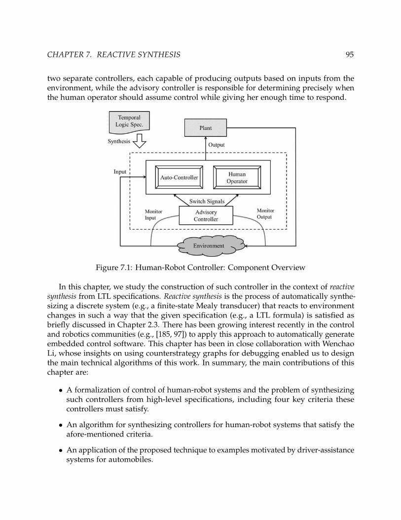
CHAPTER 7. REACTIVE SYNTHESIS 95
two separate controllers, each capable of producing outputs based on inputs from theenvironment, while the advisory controller is responsible for determining precisely whenthe human operator should assume control while giving her enough time to respond.
Figure 7.1: Human-Robot Controller: Component Overview
In this chapter, we study the construction of such controller in the context of reactivesynthesis from LTL specifications. Reactive synthesis is the process of automatically synthe-sizing a discrete system (e.g., a finite-state Mealy transducer) that reacts to environmentchanges in such a way that the given specification (e.g., a LTL formula) is satisfied asbriefly discussed in Chapter 2.3. There has been growing interest recently in the controland robotics communities (e.g., [185, 97]) to apply this approach to automatically generateembedded control software. This chapter has been in close collaboration with WenchaoLi, whose insights on using counterstrategy graphs for debugging enabled us to designthe main technical algorithms of this work. In summary, the main contributions of thischapter are:
• A formalization of control of human-robot systems and the problem of synthesizingsuch controllers from high-level specifications, including four key criteria thesecontrollers must satisfy.
• An algorithm for synthesizing controllers for human-robot systems that satisfy theafore-mentioned criteria.
• An application of the proposed technique to examples motivated by driver-assistancesystems for automobiles.


CHAPTER 7. REACTIVE SYNTHESIS 97
In general, it is not always possible to come up with a fully automatic controller thatsatisfies all requirements. Figure 7.2b illustrates such a scenario where car C blocks theview as well as the movement path of car A after two time steps. The arrow indicate themovements of the vehicles at time steps 1 and 2. Positions of a car X at time t is indicatedby Xt. In this failure scenario, the autonomous vehicle needs to notify the human driversince it has lost track of car B.
Therefore, a human-robot control synthesis problem is tasked with producing anautonomous controller along with advisories for the human driver in situations where herattention is required. Our challenge, however, is to identify the conditions that we need tomonitor and notify the driver when they may fail. In the next section, we discuss how humanconstraints such as response time can be simultaneously considered in the solution, andmechanisms for switching control between the auto-controller and the human driver.
7.2 Formal Model of Human-Robot Controller
Consider a Booleanized space over the input and output alphabet X = 2X and Y =2Y, where X and Y are two disjoint sets of variables representing inputs and outputsrespectively, we model a discrete controller as a finite-state transducer. A finite-state(Mealy) transducer (FST) is a tuple M = (Q, q0,X ,Y , ρ, δ), where Q is the set of states,q0 ∈ Q is the initial state, ρ : Q×X → Q is the transition function, and δ : Q×X → Y isthe output function. Given an input sequence x = x0, x1, . . ., a run of M is the infinitesequence q = q0, q1, . . . of states such that qk+1 = ρ(qk, ik) for all k ≥ 0. The run q on xproduces the word M(x) = δ(q0, x0)δ(q1, x1) . . .. The language of M is then denoted bythe set L(M) = (x, y)ω |M(x) = y.
To characterize correctness of M, we assume that we can label if a state is unsafe or not,by using a function F : Q→ true, false, i.e. a state q is failure-prone if F (q) = true.We elaborate on F later in Section 7.3.
Agents as Automata
We model two of the three agents in the human-robot controller shown in Figure ??,the automatic controller Auto and the advisory controller VC, as finite-state transducers(FSTs). The human operator can be viewed as another FST H that uses the same inputand output interface as the auto-controller. The overall controller is then a composition ofthe models of H, Auto and VC.
We use a binary variable auto to denote the internal advisory signal that VC sendsto both Auto and H. Hence, XH = X Auto = X ∪ auto, and YVC = auto. Whenauto = false, it means the advisory controller is requiring the human operator to takeover control, and the auto-controller can have control otherwise.
We assume that the human operator (e.g., driver behind the wheel) can take control atany time by transitioning from a “non-active” state to an “active” state, e.g., by hitting

CHAPTER 7. REACTIVE SYNTHESIS 98
a button on the dashboard or simply pressing down the gas pedal or the brake. WhenH is in the “active” state, the human operator essentially acts as the automaton thatproduces outputs to the plant (e.g., a car) based on environment inputs. We use a binaryvariable active to denote if H is in the “active” state. When active = true, the output ofH overwrites the output of Auto. The “overwrite” action happens when a sensor sensesthe human operator is in control, e.g., putting her hands on the wheel. Similarly, whenactive = false, the output of the human-robot controller is the output of Auto. Note thateven though the human operator is modeled as a FST here, since we do not have directcontrol of the human operator, it can in fact be any arbitrary relation mapping X to Y .
Criteria for Human-Robot Controllers
One key distinguishing factor of a human-robot controller from traditional controlleris the involvement of a human operator. Hence, human factors such as response timecannot be disregarded. In addition, we would like to minimize the need to engage thehuman operator. Based on the NHTSA statement, we derive four criteria for any effectivehuman-robot controller, as stated below.
• Monitoring. An advisory auto is issued to the human operator under specificconditions. These conditions in turn need to be determined unambiguously atruntime, potentially based on history information but not predictions. In a reactivesetting, this means we can use trace information only up to the point when theenvironment provides a next input from the current state.
• Minimally intervening. Our mode of interaction requires only selective humanintervention. An intervention occurs when H transitions from the “non-active”state to the “active” state (we discuss mechanisms for suggesting a transition from“active” to “non-active” in Section 7.3, after prompted by the advisory signal autobeing false). However, frequent transfer of control would mean constant attentionis required from the human operator, thus nullifying the benefits of having theauto-controller. In order to reduce the overhead of human participation, we want tominimize a joint objective function C that combines two elements: (i) the probabilitythat when auto is set to false, the environment will eventually force Auto into afailure scenario, and (ii) the cost of having the human operator taking control. Weformalize this objective function in Section 7.3.
• Prescient. It may be too late to seek the human operator’s attention when failure isimminent. We also need to allow extra time for the human to respond and study thesituation. Thus, we require an advisory to be issued ahead of any failure scenario.In the discrete setting, we assume we are given a positive integer T representinghuman response time (which can be driver-specific), and require that auto is set tofalse at least T number of transitions ahead of a state (in Auto) that is unsafe.
CHAPTER 7. REACTIVE SYNTHESIS 99
• Conditionally-Correct. The auto-controller is responsible for correct operation as longas auto is set to true. Formally, if auto = true when Auto is at a state q, thenF (q) = false. Additionally, when auto is set to false, the auto-controller shouldstill maintain correct operation in the next T − 1 time steps, during or after whichwe assume the human operator take over control. Formally, if auto changes fromtrue to false when Auto is at a state q, let RT(q) be the set of states reachable fromq within T − 1 transitions, then F (q′) = false, ∀q′ ∈ RT(q).
Problem 4 (Human-Robot Controller Synthesis Problem). Given a model of the system andits specification expressed in a formal language, synthesize a human-robot controller that is, byconstruction, monitoring, minimally intervening, prescient, and conditionally correct.
In this chapter, we study the synthesis of a human-robot controller in the setting ofsynthesis of reactive systems from Linear Temporal Logic (LTL) specifications. We givebackground on this setting in Chapter 2.3, and propose an algorithm for solving theHuman-Robot Controller Synthesis problem in Section 7.3.
7.3 Human-Robot Controller Synthesis
Given an unrealizable specification, a counterstrategy S env exists for env which describesmoves by env such that it can force a violation of the system guarantees. The key insightof our approach for synthesizing a human-robot controller is that we can synthesizean advisory controller that monitors these moves and prompts the human operatorwith sufficient time ahead of any danger. These moves are essentially assumptionson the environment under which the system guarantees can be ensured. When theseassumptions are not violated (the environment may behave in a benign way in reality),the auto-controller fulfills the objective of the controller. On the other hand, if any of theassumptions is violated, as flagged by the advisory controller, then the control is safelyswitched to the human operator in a way that she can have sufficient time to respond.The challenge, however, is to decide when an advisory should be sent to the humanoperator, in a way that it is also minimally intervening to the human operator. We use thefollowing example to illustrate our algorithm.
Example 1. Consider X = x, Y = y and the following LTL sub-formulas which togetherform ψ = ψenv → ψsys.
• ψenvf = G (F ¬x)
• ψsyst = G (¬x → ¬y)
• ψsysf = G (F y)

CHAPTER 7. REACTIVE SYNTHESIS 100
!"#$
!#$
!#
!"#$
!"% #$
!"% #$
!"% #$
!"% #$
&'
&(
&(
&(
(a) Counterstrategy graph Gc for unre-alizable specification ψ.
$
!"#$
!#$
!#
!"% #$
!"% #$
!"% #$
!"#$
&'
&(
&(
&(
failure-prone
(b) Condensed graph Gc for Gc aftercontracting the strongly connected com-ponents.
Specification ψ is not realizable. Figure 7.3a shows the computed counterstrategy graph Gc.The literal x (y) denotes the negation of the propositional variable x (y). The memory contentis denoted by γi with γ0 being the initial memory content. The three states on the left are theinitial states. The literals on the edges indicate that the environment first chooses x and thenthe system chooses y. (the system is forced to pick y due to ψ
syst ). Observe that, according the
counterstrategy, the system will be forced to pick y perpetually. Hence, the other system guaranteeψ
sysf cannot be satisfied.
Weighted Counterstrategy Graph
Recall that a counterstrategy can be viewed as a discrete transition system or a directedgraph Gc. We consider two types of imminent failures (violation of some system guaranteespecification) described by Gc.
• Safety violation. For a node (state) q1c ∈ Qc, if there does not exist a node q2
c suchthat (q1
c , q2c) ∈ ρc, then we say q1
c is failure-imminent. In this scenario, after env picksa next input according to the counterstrategy, sys cannot find a next output suchthat all of the (safety) guarantees are satisfied (some ψ
sysi or ψ
syst is violated).
• Fairness violation. If a node qc is part of a strongly connected component (SCC) inQc, then we say qc is failure-doomed. For example, the node (x, y, γ1) in Figure 7.3ais a failure-doomed node. Starting from qc, env can always pick inputs in such away that the play is forced to get stuck in SCC. Clearly, all other states in SCC arealso failure-doomed.
Now we make the connection of the labeling function F for a controller M to thecounterstrategy graph Gc which describes behaviors that M should not exhibit. Consider
CHAPTER 7. REACTIVE SYNTHESIS 101
an auto-controller M and a state q (represented by the assignment xy) in M. F (q) = true
if and only if there exist some qc ∈ Qc such that θc(qc) = xy and qc is either failure-imminent or failure-doomed. In practice, it is not always the case that the environmentwill behave in the most adversarial way. For example, a car in front may yield if itis blocking our path. Hence, even though the specification is not realizable, it is stillimportant to assess, at any given state, whether it will actually lead to a violation. Forsimplicity, we assume that the environment will adhere to the counterstrategy once itenters a failure-doomed state.
We can convert Gc to its directed acyclic graph (DAG) embedding Gc = (Qc, Q0c , ρc)
by contracting each SCC in Gc to a single node. Figure 7.3b shows the condensed graph
Gc of Gc shown in Figure 7.3a. We use a surjective function f : Qc → Qc to describe themapping of nodes from Gc to Gc. We say a node q ∈ Qc is failure-prone if a node qc ∈ Qc
is either failure-imminent or failure-doomed and f (qc) = q.Recall from Section 7.2 that the notion of minimally-intervening requires the minimiza-
tion of a cost function C, which involves the probability that auto is set to false, Thus far,we have not associated any probabilities with transitions taken by the environment or thesystem. While our approach can be adapted to work with any assignment of probabilities,for ease of presentation, we make a particular choice in this chapter. Specifically, weassume that at each step, the environment picks a next-input uniformly at random fromthe set of possible legal actions (next-inputs) obtained from ηenv given the current state.In Example 1 and correspondingly Figure 7.3a, this means that it is equally likely for envto choose x or x from any of the states. We use c(q) to denote the total number of legalactions that the environment can take from a state q.
In addition, we take into account of the cost of having the human operator performthe maneuver instead of the auto-controller. In general, this cost increases with longerhuman engagement. Based on these two notions, we define , which assigns a weight toan edge e ∈ Qc × Qc in Gc, recursively as follows. For an edge between qi and qj,
(qi, qj) =
1 if qj is failure-pronepen(qi)×len(qi)
c(qi)Otherwise
where pen : Qc → Q+ is a user-defined penalty parameter3, and len : Qc → Z+ is thelength (number of edges) of the shortest path from a node qi to any failure-prone nodein Gc. Intuitively, a state far away from any failure-prone state is less likely to cause afailure since the environment would need to make multiple consecutive moves all in anadversarial way. However, if we transfer control at this state, the human operator willhave to spend more time in control, which is not desirable for a human-robot systemcontroller. Next, we describe how to use this edge-weighted DAG representation of acounterstrategy graph to derive a controller that satisfies the criteria established earlier.
3 pen(qi) should be chosen such that (qi, qj) < 1.

CHAPTER 7. REACTIVE SYNTHESIS 102
Counterstrategy-Guided Synthesis
Suppose we have a counterstrategy graph Gc that summarizes all possible ways for theenvironment to force a violation of the system guarantees. Consider an outgoing edgefrom a non-failure-prone node q in Gc (condensed graph of Gc), this edge encodes aparticular condition where the environment makes a next-move given some last movemade by the environment and the system. If some of these next-moves by the environmentare disallowed, such that none of the failure-prone nodes are reachable from any initialstate, then we have effectively eliminated the counterstrategy. This means that if we assertthe negation of the corresponding conditions as additional ψenv
t (environment transitionassumptions), then we can obtain a realizable specification.
Formally, we mine assumptions of the form φ =∧
i(G (ai → ¬X bi)), where ai isa Boolean formula describing a set of assignments over variables in X ∪ Y, and bi is aBoolean formula describing a set of assignments over variables in X.
Under the assumption φ, if (φ ∧ ψenv)→ ψsys is realizable, then we can automaticallysynthesize an auto-controller that satisfies ψ. In addition, the key observation here is thatmining φ is equivalent to finding a set of edges in Gc such that, if these edges are removedfrom Gc, then none of the failure-prone nodes is reachable from any initial state. Wedenote such set of edges as Eφ, where each edge e ∈ Eφ corresponds to a conjunct in φ.For example, if we remove the three outgoing edges from the source nodes in Figure 7.3b,then the failure-prone node is not reachable. Removing these three edges correspond toadding the following environment assumption, which can be monitored at runtime.
G ((x ∧ y)→ ¬X x) ∧G ((x ∧ y)→ ¬X x) ∧G ((x ∧ y)→ ¬X x)
Human factors play an important role in the design of a controller for human-robotsystems. The criteria established for a controller in Section 7.2 also require it to be prescientand minimally intervening. Hence, we want to mine assumptions that reflect these criteriaas well. The notion of prescient essentially requires that none of the failure-prone nodesis reachable from a non-failure-prone node with less than T steps (edges). The weightfunction introduced earlier can be used to characterize the cost of a failing assumptionresulting in the advisory controller prompting the human operator to take over control(by setting auto to false). Formally, we seek Eφ such that the total cost of switchingcontrol ∑e∈Eφ (e) is minimized.
We can formulate this problem as a s-t min-cut problem for directed acyclic graphs.Given Gc, we first compute the subset of nodes QT
c ⊆ Qc that are backward reachablewithin T − 1 steps from the set of failure-prone nodes (when T = 1, QT
c is the set offailure-prone node). We assume that Q0
c ∩ QTc = ∅. Next, we remove the set of nodes QT
c
from Gc and obtain a new graph GTc . Since GT
c is again a DAG, we have a set of sourcenodes and a set of terminal nodes. Thus, we can formulate a s-t min-cut problem byadding a new source node that has an outgoing edge (with a sufficiently large weight)to each of the source nodes and a new terminal node that has an incoming edge (witha sufficiently large weight) from each of the terminal nodes. This s-t min-cut problem

CHAPTER 7. REACTIVE SYNTHESIS 103
Algorithm 2 Counterstrategy-Guided Human-Robot Controller Synthesis
Input: GR(1) specification ψ = ψenv → ψsys.Input: T : parameter for minimum human response time.Output: Auto and VC. Our controller is then a composition of Auto, VC and H.
if ψ is realizable thenSynthesize transducer M |= ψ (using standard LTL synthesis);Controller := M (fully autonomous).
elseGenerate Gc from ψ (assume a single Gc; otherwise the algorithm is performediteratively);Generate the DAG embedded Gc from Gc.Reduce Gc to GT
c ;Assign weights to Gc using ϕ; by removing QT
c – nodes that are within T− 1 steps ofany failure-prone node;Formulate a s-t min-cut problem with GT
c ;Solve the s-t min-cut problem to obtain Eφ;Add assumptions φ to ψ to obtain the new specification ψnew := (φ ∧ ψenv)→ ψsys;Synthesize Auto so that M |= ψnew;Synthesize VC as a (stateless) monitor that outputs auto = false if φ is violated.
end if
can be easily solved by standard techniques [40]. The overall approach is summarized inAlgorithm 2.
Theorem 4. Given a LTL specification ψ and a response time parameter T, Algorithm 2 is guar-anteed to either produce a fully autonomous controller satisfying ψ, or a human-robot controller,modeled as a composition of an auto-controller Auto, a human operator and an advisory con-troller VC, that is monitoring, prescient with parameter T, minimally intervening4 withrespect to the cost function fC = ∑e∈Eφ (e), and conditionally correct5.
Proof. (Sketch) When ψ is realizable, a fully autonomous controller is synthesized andunconditionally satisfies ψ. Now consider that case when ψ is not realizable.
The HuIL controller is monitoring as φ only comprises a set of environment transitionsup to the next environment input.
It is prescient by construction. The auto flag advising the human operator to take overcontrol is set to false precisely when φ is violated. When φ is violated, it corresponds tothe environment making a next-move from the current state q according to some edge
e = (qi, qj) ∈ Eφ. Consider any qc ∈ Qc such that f (qc) = qi, θc(qc) = q. Since qi 6∈ QTc by
4We assume the counterstrategy we use to mine the assumptions is an optimal one – it forces a violationof the system guarantees as quickly as possible.
5We assume that all failure-prone nodes are at least T steps away from any initial node.

CHAPTER 7. REACTIVE SYNTHESIS 104
the construction of GTc , qi is at least T transitions away from any failure-prone state in Gc.
This means qc must also be at least T transitions away from any failure-imminent state orfailure-doomed state in Qc. Hence, by the definition of F with respect to a failure-doomedor failure-doomed state in Section 7.3, q is (and auto is set) at least T transitions ahead ofany state that is unsafe.
The controller is also conditionally correct. By the same reasoning as above, for anystate q′ ∈ RT(q), F (q′) = false, i.e. q′ is safe.
Finally, since auto is set to false precisely when φ is violated, and φ in turn isconstructed based on the set of edges Eφ, which minimizes the cost function fC =∑e∈Eφ (e), the controller is minimally-intervening with respect to the cost function fC.
Switching from Human Operator to Auto-Controller
Once control has been transferred to the human operator, when should the human yieldcontrol to the autonomous controller again? One idea is for the controller to continuallymonitor the environment after the human operator has taken control, checking if a stateis reached from which the auto-controller can ensure that it satisfies the specification(under assumption φ), and then the advisory controller can signal a driver telling her thatthe auto-controller is ready to take back control. We note that alternative approaches mayexist and we plan to investigate this further in future work.
7.4 Experimental Results
Our algorithm is implemented as an extension to the GR(1) synthesis tool RATSY [30]. Wenow discuss the car-following example (as shown in Section 7.1) here. The implementationcan be found here: http://verifun.eecs.berkeley.edu/tacas14/
Recall the car-following example shown in Section 7.1. We describe some of the moreinteresting specifications below and their corresponding LTL formulas. pA, pB, pC areused to denote the positions of car A, B and C respectively.
• Any position can be occupied by at most one car at a time (no crashing):
G(
pA = x → (pB 6= x ∧ pC 6= x))
where x denotes a position on the discretized space. The cases for B and C aresimilar, but they are part of ψenv.
• Car A is required to follow car B:
G(
(vAB = true ∧ pA = x)→ X (vAB = true))
where vAB = true if and only if car A can see car B.
CHAPTER 7. REACTIVE SYNTHESIS 105
• Two cars cannot cross each other if they are right next to each other. For example,when pC = 5, pA = 6 and p′C = 8 (in the next cycle), p′A 6= 7. In LTL,
G(
((pC = 5) ∧ (pA = 6) ∧ (X pC = 8))→ (X (pA 6= 7)))
The other specifications can be found in the link at the beginning of this section.Observe that car C can in fact force a violation of the system guarantees in one step undertwo situations – when pC = 5, pB = 8 and pA = 4, or pC = 5, pB = 8 and pA = 6. Bothare situations where car C is blocking the view of car A, causing it to lose track of car B.The second failure scenario is illustrated in Figure 7.2b.
Applying our algorithm to this (unrealizable) specification with T = 1, we obtain thefollowing assumption φ.
φ = G(
((pA = 4) ∧ (pB = 6) ∧ (pC = 1))→ ¬X ((pB = 8) ∧ (pC = 5)))∧
G(
((pA = 4) ∧ (pB = 6) ∧ (pC = 1))→ ¬X ((pB = 6) ∧ (pC = 3)))∧
G(
((pA = 4) ∧ (pB = 6) ∧ (pC = 1))→ ¬X ((pB = 6) ∧ (pC = 5)))
In fact, φ corresponds to three possible evolutions of the environment from the initialstate. In general, φ can be a conjunction of conditions at different time steps as env andsys progress. The advantage of our approach is that it can produce φ such that we cansynthesize an auto-controller that is guaranteed to satisfy the specification if φ is notviolated, together with an advisory controller that prompts the driver (at least) T (T = 1in this case) time steps ahead of a potential failure when φ is violated.
7.5 Chapter Summary
ln this chapter, we’ve discussed the problem of reactive synthesis from temporal logicspecifications [141, 138]. Similar to [97], we have synthesized a discrete controller fromtemporal logic specifications.
Wongpiromsarn et al. [183] consider a receding horizon framework to reduce thesynthesis problem to a set of simpler problems for a short horizon. We further discuss areceding horizon variant of our problem in the future chapters. Livingston et al. [112, 113]exploit the notion of locality that allows “patching" a nominal solution. They update thelocal parts of the strategy as new data accumulates allowing incremental synthesis. Thepatching algorithm considers changes in the game graph, and identifies the affected nodesfor each system goal and modifies the graph locally. In our approach, we do not start witha synthesized game graph, and we mine assumptions from counterstrategies. Also, weconsider environment assumptions that are not only limited to the topological changes.The key innovation in this chapter is that our work is the first to consider synthesizinginterventions that combine an autonomous controller with a human operator.
CHAPTER 7. REACTIVE SYNTHESIS 106
Our work is inspired by the recent works on assumption mining. Chatterjee et al. [37]construct a minimal environment assumption by removing edges from the game graphto ensure safety assumptions, then compute liveness assumptions to put additionalfairness constraints on the remaining edges. Finding this minimal set is NP-Hard.Our approach is based on removing edges from the counter-strategy; therefore, theenvironment assumptions are easier to mine, and more practical as they can be mappedto monitoring real sensors. The flexibility of choosing which edge to remove gives us ameasure of conservativeness in our control. Removing edges closer to the source nodeprevents any violations in the future moves and removing edges towards the sink nodeis less conservative. Li et al. [109] and later Alur et al. [8] use a counterstrategy-guidedapproach to mine environment assumptions for GR(1) specifications. We adapt thisapproach to the synthesis of controllers for human-robot systems.
Finally, human’s reaction time while driving is an important consideration in thischapter. This time is based on human’s reaction time while driving, which is driver-specific. The value of reaction time can range from 1 to 2.5 seconds for different tasksand drivers [169].
One limitation of the current approach is the use of an explicit counterstrategy graph(due to weight assignment). We plan to explore symbolic algorithms in the future. Further,we plan to synthesize a systematic intervention scheme that closely combines models ofoperators, and provides formal correctness guarantees about it.

107
Chapter 8
Reactive Synthesis from SignalTemporal Logic
In this chapter, our goal is to design controllers that satisfy desired temporal logicspecifications despite a potentially adversarial environment or human models. Thesesynthesized controllers are robust to uncertain environment or human actions.
As we have seen in the previous chapter, temporal logics is a valuable tool forcontroller synthesis. Approaches using temporal logic can be broadly categorized basedon if they use a discrete abstraction of the system, and if the environment is assumed tobe deterministic.
Using discrete abstraction enables the construction of a discrete supervisory controller,which can then construct a hybrid controller. These discrete abstraction techniquesaddress both deterministic [94, 133] and adversarial environments [53, 186]. In contrast,techniques that avoid discrete abstraction include sampling-based methods [88], andmixed-integer linear programming encodings of temporal logic specifications [86, 89, 100,182, 147].
In this chapter, we plan to close the gap between these two techniques by addressingcontroller synthesis under reactive environments through mixed-integer linear program-ming encodings. The ideas and results of this chapter was done in close collaborationwith Vasumathi Raman, Alexandre Donze, Richard Murray, and Sanjit Seshia. Specifically,Vasumathi Raman’s ideas for the mixed integer encoding of signal temporal logic, andher previous work [146] has provided us with an insight that led to the algorithms andresults of this chapter.
We adopt a counterexample-guided inductive synthesis [166] approach to synthesize acontroller satisfying reactive specifications. Inductive synthesis refers to the automatedgeneration of a system from input-output examples, using each new example to iterativelyrefine the hypothesis about the system until convergence. In Counterexample-GuidedInductive Synthesis (CEGIS), the examples are mostly counterexamples discovered whiletrying to verify correctness of the current guess. CEGIS thus relies primarily on avalidation engine to validate candidates produced at intermediate iterations, which can

CHAPTER 8. REACTIVE SYNTHESIS FROM STL 108
produce counterexamples for use in the next iteration. Automated synthesis of systemsusing CEGIS and the closely related Counterexample-Guided Abstraction Refinement(CEGAR) paradigm has been widely studied in various contexts [38, 8, 84].
The specification language adopted here is STL [119], which allows the specificationof temporal properties of real-valued signals, and has been applied to the analysis ofhybrid dynamical systems from various application domains such as analog and mixedsignal circuits, systems biology or Cyber-Physical Systems (CPS) (see Chapter 2.3). Weexploit the quantitative semantics of STL to compute the robustness of satisfaction in thevalidation engine for our CEGIS approach to reactive synthesis.
A key advantage of temporal logic over, e.g., domain-specific languages based onpropositional logic, is that it enables the expression of properties of infinite traces. Wewould therefore like to synthesize controllers that can run indefinitely, and satisfy infinite-horizon properties. However, in this chapter we use a Receding Horizon Control approachintroduced in Chapter 2.1. This not only reduces computational complexity, but alsoimproves robustness with respect to exogenous disturbances and modeling uncertaintiesby allowing new information to be incorporated as it becomes available [126].
The connection between Receding Horizon Control (RHC) and control synthesis fromSTL specifications are discussed in previous work [147], where the authors specify desiredproperties of the system using a STL formula, and synthesize control strategies such thatthe system satisfies that specification, while using a receding horizon approach. Raman etal. present automatically-generated Mixed Integer Linear Program (MILP) encodings forSTL specifications, extending the Bounded Model Checking (BMC) paradigm for finitediscrete systems [28] to STL. These encodings can be used not only to generate open-loopcontrol signals that satisfy finite and infinite horizon STL properties, but also to generatesignals that maximize quantitative (robust) satisfaction. In this chapter, we show how therobustness-based encoding can be used to produce a validation engine that synthesizescounterexamples to guide a CEGIS approach to reactive synthesis.
Abbas et al. [1] exploit the quantitative semantics of Metric Temporal Logic (MTL) todesign a framework for specification-guided testing of stochastic cyber-physical systems.Leveraging results from stochastic optimization, they frame the verification of propertieson such systems as a global optimization problem of minimizing the expected robustnessof satisfaction. While we work with nondeterministic systems rather than stochasticsystems, our CEGIS approach leverages a similar idea when finding an adversarialenvironment input that minimizes the robustness of satisfaction.
Receding horizon control that satisfies temporal logic specifications in adversarialsettings has been considered before in the context of Linear Temporal Logic (LTL) [186],where the authors propose a framework utilizing discrete abstractions to synthesize su-pervisory controllers for specifications in the GR(1) subset of LTL. In this work, feasibilityof the global specification is determined via symbolic checks on a series of pre-definedsmaller problems, and strategies extracted as needed. In contrast, we do not require an apriori defined finite set of sub-problems. Our approach also extends synthesis capabilitiesto a wider class of temporal logic specifications and environments than [68, 23], and

CHAPTER 8. REACTIVE SYNTHESIS FROM STL 109
avoids potentially expensive computations of a finite state abstraction of the system as in[43] and [186].
The key contribution of this chapter is a CEGIS approach to controller synthesis forcyber-physical systems subject to signal temporal logic (STL) specifications, operating inand interacting with potentially adversarial nondeterministic environments or humanagents. Specific features of our approach include:
• We leverage the previously-proposed encoding of STL specifications as mixedinteger-linear constraints [147], and solve a counterexample-guided series of opti-mization problems to yield a satisfying control sequence.
• Our framework can be used in a receding horizon fashion to fulfill properties overunbounded horizons.
• We present experimental results using a case study of controller synthesis for anautonomous driving scenario in the presence of adversarial agents; simulationresults in this domain illustrate the effectiveness of our methodology.
8.1 MILP Encoding for Controller Synthesis
In order to synthesize a run that satisfies a STL formula ϕ, we add STL constraints toa MILP formulation of the control synthesis problem as in [147]. We first represent thesystem trajectory as a finite sequence of states satisfying the model dynamics in equation(2.7). Then, we encode the formula ϕ with a set of MILP constraints; our encodingproduces a MILP as long as the functions µ that define the predicates πµ in ϕ are linearor affine.
Constraints on system evolution
The system constraints encode valid finite (horizon-N) trajectories for a dynamical system–these constraints hold if and only if the trajectory ξ(x0, uN, wN) satisfies (2.7). A typicalsituation is when the discrete dynamics fd is linear. In that case, the constraints on systemevolution are of the form
x1 = Ax0 + Buu0 + Bww0
x2 = Ax1 + Buu1 + Bww1
. . .
xN = AxN−1 + BuuN−1 + BwwN−1

CHAPTER 8. REACTIVE SYNTHESIS FROM STL 110
STL constraints
The robustness of satisfaction of the STL specification, as defined in Chapter 2.3, providesa natural objective for the MILP defined above, either in the absence of, or as a complementto domain-specific objectives on runs of the system.
As described in Chapter 2.3, the robustness of a STL specification ϕ can be computedrecursively on the structure of the formula. Moreover, since max and min operationscan be expressed in a MILP formulation using additional binary variables, this doesnot add complexity to the encoding (although the additional variables make it morecomputationally expensive in practice). For a given formula ϕ, we introduce a variable ρ
ϕk ,
and an associated set of MILP constraints such that ρϕk > 0 if and only if ϕ holds at time tk.
Given ϕ, we recursively generate MILP constraints for every subformula of ϕ, such thatρ
ϕ0 determines whether ϕ holds in the initial state. For example, enforcing ρ
ϕk = ρϕ(x, tk)
gives us this property. The reader is referred to [147] for details of this encoding. Theadvantage of this robustness-based encoding is that it allows us to maximize or minimizethe value of ρ
ϕ0 , obtaining a trajectory that maximizes or minimizes the robustness of
satisfaction.The union of the STL constraints and system constraints yields a MILP, enabling us
to check feasibility and find a solution when possible using a MILP solver; for furtherdetails and examples see [147]. Given an objective function on runs of the system, wecan also find an optimal trajectory that satisfies the STL specification. The robustnessprovides a natural objective for this MILP, either in the absence of, or as a complement todomain-specific objectives on runs of the system.
Mixed integer-linear programs are NP-hard, and hence impractical when the dimen-sions of the problem grow. We present the computational costs of the above encoding interms of the number of variables and constraints in the resulting MILP. If P is the set ofpredicates used in the formula and |ϕ| is the length (i.e. the number of operators), thenO(N · |P|) + O(N · |ϕ|) continuous variables are introduced. In addition, O(N) binaryvariables are introduced for every instance of a Boolean operator, i.e., O(N · |ϕ|) Booleanvariables.
The dimensionality of the discrete-time dynamical system affects the size of theconstructed MILP linearly via the constraints encoding system evolution (more precisely,through the size of the set of predicates P). However, given the efficiency of modernMILP solvers, there is no evidence that a linear increase in the problem size would inpractice lead to more than a linear increase in computational time for a solution. Methodsbased on abstraction or discretization of the state space, on the other hand, are muchmore likely to have exponential complexity with respect to system dimensionality. Wenote, however, that our approach is more sensitive to the size of the specifications, and inparticular to the nesting degree of temporal operators. We report on the scalability of ourapproach in Section 8.5.

CHAPTER 8. REACTIVE SYNTHESIS FROM STL 111
8.2 STL Reactive Synthesis Problem
We address the problem of synthesizing control inputs for a system operating in thepresence of potentially adversarial, a priori uncertain external inputs or disturbances. Thecontrollers we produce will provide guarantees for specifications of the form ϕ
.= ϕe ⇒ ϕs,
where ϕe places assumptions on the external environment, and ϕs specifies desiredguarantees on the plant behavior. In this chapter, ϕe refers exclusively to properties ofsignals w ∈Wω, whereas ϕs refers to properties of x ∈ X ω and u ∈ Uω.
We now formally state the synthesis problem for reactive controllers subject to STLspecifications of the form above, and its receding horizon formulation.
Problem 5 (STL Reactive Synthesis). Given a discrete dynamical system:
xt+1 = f (xt, ut, wt), (8.1)
initial state x0, trajectory length N, STL formula ϕ and cost function J, compute:
argminuN
maxwN∈w∈WN |w|=ϕe
J(ξ(x0, uN, wN))
s.t. ∀wN ∈WN, ξ(x0, uN, wN) |= ϕ
Problem 6 (Receding Horizon Reactive Synthesis). Given a system of the form in equation(8.1), initial state x0, STL formula ϕ and cost function J, at each time step k, compute:
argminuH,k
maxwH,k∈w∈WH |w|=ϕe
J(ξ(xk, uH,k, wH,k))
s.t. ∀w ∈Wω, ξ(x0, u, w) |= ϕ,
where H is a finite horizon provided as a user input or selected in some other fashion, uH,k is the
horizon-H control input computed at each time step and u = uH,00 uH,1
0 uH,20 ....
In Sections 8.3 and 8.4, we present both a finite-trajectory solution to Problem 5,and a solution to Problem 6 for a large class of STL formulas. A key component ofour solution is to use the previously presented encoding of STL specifications as MILPconstraints [147] in combination with MILP constraints representing the system dynamicsto efficiently solve the resulting constrained optimization problem.
8.3 Counterexample-Guided Finite Horizon Synthesis
We propose a solution to Problem 5 using a counterexample guided inductive synthesis(CEGIS) procedure. We first consider bounded STL properties ϕ, bounded by N ∈ N.

CHAPTER 8. REACTIVE SYNTHESIS FROM STL 112
Algorithm 3 CEGIS Algorithm for Problem 5
1: Input: ξ, x0, N, ϕ, J2: Let w0 = (w0
1, w02, ...w0
N−1), s.t. wN |= ϕe
3: Wcand = w04: while True do5:
u0 ← argminu∈UN
maxw0∈WcandJ(ξ(x0, u, w0))
s.t. ∀w0 ∈Wcand, ξ(x0, u, w0) |= ϕs,
6: if u0 == null then7: Return INFEASIBLE
8: end if9:
w1 ← argminw∈WN ρϕ(ξ(x0, u0, w), 0)s.t. w1 |= ϕe
10: if ρϕ(ξ(x0, u0, w1)) > 0 then11: Return u0
12: else13: Wcand ←Wcand ∪ w114: end if15: end while
Once we have this scheme for synthesizing control for finite trajectories satisfying boundedspecifications, we will use a receding horizon scheme for infinite trajectories.
We now describe the steps of Algorithm 3 in detail. In Step 2, we choose an initialinstance w0 of an environment that satisfies the specification ϕe. We do so using theopen-loop synthesis algorithm for bounded-time STL described in [147]. Our initial setof candidate environment inputs is a singleton, Wcand = w0 (Step 3). Then, in Step 5,we compute the optimal control input u0 with respect to this environment, such that thesystem specification ϕs is satisfied; this step also uses the solution in [147]. If the problemin Step 5 is infeasible, we know that there is a control input w0 ∈Wcand against which nocontrol input can satisfy ϕ, so we can stop and return (Step 7). Otherwise, in Step 9, wefind an environment w1 that satisfies ϕe, but also minimizes the robustness of satisfactionof ϕ for the control input u0. Essentially, this step tries to find an environment thatfalsifies the specification ϕ when the control input u0 is used. If the minimum robustnessρϕ(ξ(x0, u0, w1)) thus computed is positive, this implies ∀w ∈WN ξ(x0, u0, w) |= ϕ, sowe can return the control input u0 as our result in Step 11. Otherwise, we have generateda counterexample to u0 being the desired control input, i.e. an environment w1 thatfalsifies ϕ when u0 is used. We use this counterexample to guide our inductive synthesisin Step 13, by adding it to the set of environments to be considered in the next iteration.

CHAPTER 8. REACTIVE SYNTHESIS FROM STL 113
We then resume execution of the while loop from Step 4.
Theorem 5. If Algorithm 3 returns uN ∈ UN, then ∀wN ∈ WN, ξ(x0, uN, wN) |= ϕ. IfAlgorithm 3 returns INFEASIBLE, then Problem 5 is infeasible.
Note that Algorithm 3 does not fully solve Problem 5, because it does not alwaysensure cost-optimality of uN with respect to all disturbances wN ∈WN — the returneduN is optimal with respect to a specific set of disturbances Wcand ⊆ WN.
Since |Wcand| grows by 1 at every iteration of the while loop, the MILP in Step 5grows linearly with the number of iterations, as we duplicate constraints for each newcounterexample. If W is finite, Wcand will converge, and Algorithm 3 is sound andcomplete.
If W is infinite, Algorithm 3 may never terminate. We can choose to execute amaximum number of iterations of the while loop before declaring the problem infeasible.However, there is actually more information available to us. In fact, we can solve therobust control problem (i.e. Problem 5) to within an arbitrary tolerance by samplinga finite number of independent and identically distributed (i.i.d.) wN. Esfahani et al.show the feasibility and performance bound of this approach for a class of non-convexMILP problems [49]. They prove that for this specific class of programs, the quality ofthe solution after drawing M i.i.d. samples can be lower-bounded. Here, we first showthat we can have a similar bound by i.i.d. sampling, and then prove that Algorithm 3performs strictly better than i.i.d. sampling. We first formulate Problem 5 as a feasibilityproblem by moving the objective to the set of constraints. This transformation facilitatesdefining a relaxed variant of Problem 5.
Problem 7. Given a system of the form in equation (8.1), initial state x0, trajectory length N,STL formula ϕ, cost function J, and threshold t compute:
argminuN
0
s.t. ∀wN ∈WN, ξ(x0, uN, wN) |= ϕ,∀wN ∈ w ∈WN |w |= ϕe J(ξ(x0, uN, wN)) ≤ t.
Now, we define an ǫ-relaxation of Problem 7, where each constraint is satisfied withinan ǫ threshold.
Problem 8 (Relaxed STL Reactive Synthesis). Given a system of the form in equation (8.1),initial state x0, trajectory length N, STL formula ϕ, cost function J, and threshold t, compute:
argminuN
0
subject to ∀wN ∈WN, ξ(x0, uN, wN) |=ǫ ϕ,
∀wN ∈ w ∈WN |w |= ϕe J(ξ(x0, uN, wN)) ≤ t + ǫ,
(8.2)
where the relaxed constraint ξ(x0, uN , wN) |=ǫ ϕ represents the ǫ-satisfaction of the STL formulaϕ, which is equivalent to ρϕ(ξ(x0, uN, wN)) > −ǫ.
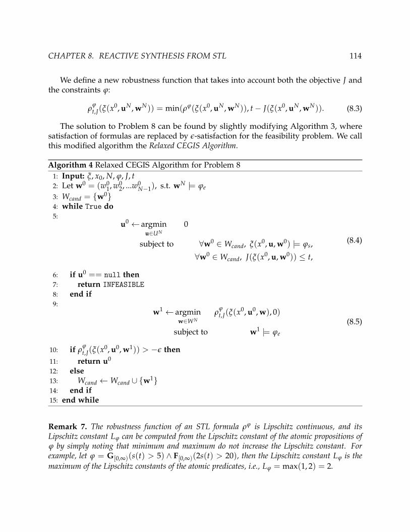
CHAPTER 8. REACTIVE SYNTHESIS FROM STL 114
We define a new robustness function that takes into account both the objective J andthe constraints ϕ:
ρϕt,J(ξ(x0, uN, wN)) = min(ρϕ(ξ(x0, uN, wN)), t− J(ξ(x0, uN, wN)). (8.3)
The solution to Problem 8 can be found by slightly modifying Algorithm 3, wheresatisfaction of formulas are replaced by ǫ-satisfaction for the feasibility problem. We callthis modified algorithm the Relaxed CEGIS Algorithm.
Algorithm 4 Relaxed CEGIS Algorithm for Problem 8
1: Input: ξ, x0, N, ϕ, J, t2: Let w0 = (w0
1, w02, ...w0
N−1), s.t. wN |= ϕe
3: Wcand = w04: while True do5:
u0 ← argminu∈UN
0
subject to ∀w0 ∈Wcand, ξ(x0, u, w0) |= ϕs,
∀w0 ∈Wcand, J(ξ(x0, u, w0)) ≤ t,
(8.4)
6: if u0 == null then7: return INFEASIBLE
8: end if9:
w1 ← argminw∈WN
ρϕt,J(ξ(x0, u0, w), 0)
subject to w1 |= ϕe
(8.5)
10: if ρϕt,J(ξ(x0, u0, w1)) > −ǫ then
11: return u0
12: else13: Wcand ←Wcand ∪ w114: end if15: end while
Remark 7. The robustness function of an STL formula ρϕ is Lipschitz continuous, and itsLipschitz constant Lϕ can be computed from the Lipschitz constant of the atomic propositions ofϕ by simply noting that minimum and maximum do not increase the Lipschitz constant. Forexample, let ϕ = G[0,∞)(s(t) > 5) ∧ F[0,∞)(2s(t) > 20), then the Lipschitz constant Lϕ is the
maximum of the Lipschitz constants of the atomic predicates, i.e., Lϕ = max(1, 2) = 2.

CHAPTER 8. REACTIVE SYNTHESIS FROM STL 115
Remark 8. Under the assumption that the objective function J is Lipschitz continuous, withLipschitz constant LJ , we define the Lipschitz constant of ρ
ϕt,J to be the maximum of Lϕ and LJ ,
i.e., L = max(LJ , Lϕ).
Lemma 3. After running the Relaxed CEGIS Algorithm for k time steps, the pairwise distancebetween wi and wj ∈ w1, . . . , wk is at least ǫ
L , where L is the Lipschitz constant of the
robustness function ρϕt,J .
Proof. We use a proof by contradiction method for Lemma 3. Without loss of generality,we assume that i < j. Let uj be the control input selected at iteration j, and wi be thedisturbance input selected at iteration i. Then, we have ρ
ϕt,J(ξ(x0, uj, wi)) > 0. Further, we
assume the distance between wi and wj is less than ǫL , i.e., |wi −wj| < ǫ
L . Therefore, by
Lipschitz continuity of ρϕt,J , we conclude:
ρϕt,J(ξ(x0, uj, wi)) >
−ǫ
L× L = −ǫ (8.6)
This contradicts our assumption, since if ρϕt,J(ξ(x0, uj, wi)) > −ǫ, Step 10 of the Relaxed
CEGIS Algorithm 4 would have returned uj.
Theorem 6. If Wcand is an ǫL cover of WN, then solving Problem 7 (or equivalently Problem 5),
where WN is replaced by Wcand provides a solution to the Relaxed STL Reactive Synthesis problem(Problem 8).
Proof. Suppose solving Problem 7 with a finite number of w ∈ Wcand returns u∗. SinceWcand is an ǫ
L cover of WN, for every w ∈WN, there exists w′ ∈Wcand and |w−w′| < ǫL .
Since u∗ is a solution of Problem 7, we have ρϕt,J(ξ(x0, u∗, w′)) > 0. By Lipschitz continuity:
|w−w′| < ǫ
L→ |ρϕ
t,J(ξ(x0, u∗, w))− ρϕt,J(ξ(x0, u∗, w′))| < ǫ. (8.7)
Therefore, ρϕt,J(ξ(x0, u∗, w)) > −ǫ for any w ∈ WN, which provides a solution to the
Relaxed STL Reactive Synthesis problem (Problem 8).
Theorem 7. Let WN = [0, 1]N. Then, an ǫL cover of WN is obtained with Θ(( L
ǫ )N log( L
ǫ )) i.i.d.samples.
Proof. We first prove that we can lower bound the number of i.i.d. samples by Ω(( Lǫ )
N log( Lǫ )).
We divide the cube [0, 1]N into ( L2ǫ )
N subcubes of side length 2ǫL , where the center of
each subcube is ǫL far from the side of the subcube. To cover the centers of the subcubes,
we need to have selected at least one point from each subcube. Therefore, the problemreduces to the coupon collector’s problem [125], where the number of coupons is the numberof subcubes, i.e., Θ(( L
ǫ )N) (for a constant N). Then, the expected number of samples
required to cover the centers of the subcubes is Ω(( Lǫ )
N log( Lǫ )) with i.i.d. sampling. So
this implies that to find an ǫL cover of WN we need Ω(( L
ǫ )N log( L
ǫ )).

CHAPTER 8. REACTIVE SYNTHESIS FROM STL 116
Now, we show that this bound is also an upper bound. We now choose the subcubeswith side length ǫ√
N·L . The diameter of such a subcube is ǫL . Therefore, if we pick one
point from each subcube, these points form an ǫL cover. Then, using the coupon collector’s
problem, we only need O(( Lǫ )
N log( Lǫ )) samples.
As we have shown both the upper and lower bounds, we only need Θ(( Lǫ )
N log( Lǫ ))
samples to cover the cube [0, 1]N.
Remark 9. If WN = [0, 1]N and Wcand is selected by i.i.d. sampling , then O(( Lǫ )
N log( Lǫ ))
samples are enough to ensure that the solution to Problem 5 with WN replaced with Wcand is asolution of Problem 8.
Theorem 8. The Relaxed CEGIS Algorithm 4 requires at most O(( Lǫ )
N) samples (under the
assumption that WN = [0, 1]N) to terminate.
Proof. We can divide the cube WN = [0, 1]N to subcubes of side length ǫ√N·L . By Lemma 3,
we only select one wi ∈ Wcand for each subcube during the CEGIS loop. Therefore, thenumber of samples is at most the number of subcubes, i.e., O(( L
ǫ )N).
Theorem 9. Any solution returned by Algorithm 4 is a feasible solution for Problem 8. Further,if Problem 7 has a feasible solution, Algorithm 4 will never return infeasible.
Proof. Step 10 of Algorithm 4 enforces that ρϕt,J(ξ(x0, u0, w1)) > −ǫ; therefore, any solu-
tion returned satisfies the feasibility of Problem 8. In addition, if Problem 7 is feasible,Step 5 of Algorithm 4 can never return infeasible.
Remark 10. If WN is bounded, then Algorithm 4 terminates in a finite number of steps. This isbecause a bounded WN can be covered by balls of diameter ǫ
L , and Wcand cannot take more thanone point in each of these balls.
Remark 11. One might be discouraged by the seemingly modest improvement of the RelaxedCEGIS Algorithm 4 over i.i.d. sampling. In fact, one might think that this improvement isoffset by the more complicated and time-consuming way of choosing w. However, we solve theoptimization problem of choosing u by reducing the problem to a MILP whose size scales linearlyin the size of Wcand. Therefore, keeping this length of Wcand as small as possible is beneficial.
In practice, solving the problem in Step 5 becomes expensive as Wcand grows, inparticular because the objective is now non-linear. While state-of-the-art MILP solvers e.g.Gurobi1 handle nonlinear objective functions efficiently, we can preserve the difficulty ofthe problem at each iteration by setting Wcand = w1 in Step 13 instead of growing theset of candidates. This breaks completeness even for finite sets W, since we may oscillatebetween two disturbances, but preserves soundness with respect to the satisfaction of ϕ,while allowing faster solutions at each iteration of the loop.
1http://www.gurobi.com/

CHAPTER 8. REACTIVE SYNTHESIS FROM STL 117
In the case study described in Section 8.5, we find that a few number of iterationsthrough the while loop suffices to either find a satisfying control input or render theproblem infeasible.
8.4 Receding Horizon Controller Synthesis in an
Adversarial Environment
In this section, we will describe a solution to Problem 6 by adding STL constraints to areceding horizon control framework. At each step t of the computation, we will employthe CEGIS approach in Section 8.3 to find a finite trajectory of fixed horizon length H,such that the trajectory accumulated over time satisfies ϕ.
Note that this problem is relatively simple for bounded-time STL formulas ϕ, asdescribed in [147]. Here the length of the horizon H is chosen to be at least the boundof formula ϕ. Then, at time step 0, we synthesize control uH,0 using the formulation
in Section 8.3, and execute only the first time step uH,00 ; we then observe wH,0
0 and x1. Then
at the next step, we solve for uH,1, while constraining the values of uH,10 = uH,0
0 , wH,10 =
wH,00 in the MILP, and retaining the STL constraints on the trajectory up to time H.
Keeping track of the history in this manner ensures that the formula is satisfied over thelength-H prefix of the trajectory, while solving for uH,t at every time step t.
Suppose that we have a specification ψ = Gϕ, where ϕ is a bounded-time formulawith bound H. In this case, we can stitch together trajectories of length H using a recedinghorizon approach to produce an infinite computation that satisfies the STL formula. Ateach step of the receding horizon computation, we search for a finite trajectory of horizonlength 2H, keeping track of the past values and robustness constraints necessary todetermine satisfaction of ψ at every time step in the trajectory.
First we define a procedure:
CEGIS∗(ξ, x0, N, ψ = Gϕ, J, PH, ukold) (8.8)
that takes additional inputs P = P0, P1, ..., PH−1 and ukold = uk
old0uk
old1...uk
oldk−1, and is
identical to Algorithm 3, except that the optimization problem in Step 5 is solved withthe added constraints:
ρϕ(ξ(x0, u, w0), i) > Pi ∀i ∈ [0, H − 1]
ui = ukoldi
∀i < k(8.9)
Algorithm 3 (CEGIS) solves reactive synthesis for bounded horizon formulas. Weare designing Algorithm 5 to deal with unbounded formulas, by invoking bounded-horizon synthesis at each time step. To ensure soundness of this infinite-horizon synthesisalgorithm, some history needs to be carried forth from one horizon to another to ensureconsistency between the newly synthesized inputs and those produced in previous steps.

CHAPTER 8. REACTIVE SYNTHESIS FROM STL 118
This is achieved by the two additional arguments of CEGIS∗ and the corresponding addedconstraints. The first constraint enforces satisfaction of ϕ at all time steps i ∈ [0, H − 1].The second constraint fixes the first k values of the newly computed input to valuescomputed in the previous time step.
Given CEGIS∗, we define a receding horizon control procedure as in Algorithm 5. Ateach time step, we compute control inputs over a horizon of 2H.
Algorithm 5 RHC Algorithm for Problem 6
1: Input: ξ, x0, ψ = Gϕ, J2: Let M be a large positive constant.3: Let H be the bound of ϕ.4: Set P0 = 0 and Pi = −M ∀ 0 < i ≤ H.5: Compute u0 = u0
0u01....u0
2H−1 as:
u0 ← CEGIS∗(ξ, x0, 2H, G[0,H]ϕ, J, PH, ∅)
6: for k = 1; k < H; k = k + 1 do7: Set uk
old = u00u1
1u22...uk−1
k−1.
8: Set Pi = 0 for 0 ≤ i ≤ k, Pi = −M ∀k < i ≤ H.9: Compute uk = uk
0uk1....uk
2H−1 as:
uk ← CEGIS∗(ξ, xk, 2H, G[0,H]ϕ, J, PH, ukold)
10: end for11: while True do12: Set uk
old = uk−11 uk−1
2 uk−13 ...uH−1
H .
13: Set Pi = 0 for 0 ≤ i ≤ H.
uk ← CEGIS∗(ξ, xk, 2H, G[0,H]ϕ, J, PH, ukold)
14: k = k + 115: end while
Algorithm 5 has two phases, a transient phase (Lines 4-10) and a stationary phase(Lines 11-14). The transient phase applies until an initial control sequence of lengthH has been computed, and the stationary phase follows. In the transient phase, thenumber of stored previous inputs (uk
old) as well as the number of time steps at whichformula ϕ is enforced (i.e. time steps for which Pi = 0) grows by one at each iteration,until they both attain a maximum of H at iteration H. Every following iteration uses awindow of size H for stored previous inputs, and sets all Pi = 0. The size-H window of

CHAPTER 8. REACTIVE SYNTHESIS FROM STL 119
previously-computed inputs advances forward one step in time at each iteration afterstep H. In this manner, we keep a record of the previously computed inputs required toensure satisfaction of ϕ up to H time steps in the past.
Theorem 10. Let u∗ be the infinite sequence of control inputs generated by setting u∗k = ukH,
where uk = uk0uk
1...uk2H−1 is the control input sequence of length 2H generated by Algorithm 5
at time tk. Then ∀w ∈Wω, ξ(x0, u∗, w) |= ψ.
Proof. Since H is the bound of ϕ, the satisfaction of ϕ at time k is established by thecontrol inputs u∗k . . . u∗k+H−1.
At time k + H,
uk+Hold = uk+H
0 uk+H1 uk+H
2 ...uk+HH−1
= uk+H−11 uk+H−1
2 uk+H−13 ...uk+H−1
H−1 uk+H−1H
= uk+H−22 uk+H−2
3 uk+H−24 ...uk+H−2
H uk+H−1H
= · · ·= uk
Huk+1H uk+2
H ...uk+H−1H
= u∗k u∗k+1u∗k+2...u∗k+H−1
and so all the inputs required to determine satisfaction of ϕ at time k have been fixed.
Moreover, if uk+H is successfully computed, then by the correctness of Algorithm 3, uk+Hold
has the property that ∀wH ∈ WH, ξ(xt, uk+Hold , wH) |= ϕ. Since uk
Huk+1H uk+2
H ...uk+H−1H =
uk+Hold , we see that ∀wH ∈WH, ξ(xk, u∗k . . . u∗k+H−1, wH) |= ϕ.
It follows that ∀wω ∈Wω, ξ(x0, u∗, w) |= ϕ.
We have therefore shown how a control input can be synthesized for infinite sequencessatisfying ψ, by repeatedly synthesizing control for sequences of length 2H. A similarapproach applies for formulas Fϕ and ϕ U ψ, where ϕ, ψ are bounded-time.
8.5 Autonomous Driving in Nondeterministic
Environments
We now consider the problem of controlling an autonomous vehicle operating in thepresence of other, potentially adversarial vehicles.
In this example, two moving vehicles approach an intersection, which they must cross.We let the red car in Figure 8.1 be the ego vehicle (the vehicle we control), and the blackcar be part of the environment. We define the state space using a simplified 6-dimensionalmodel, with the position of the two vehicles ((xego, yego), (xadv, yadv)) and the velocityof the two (vego = yego, vadv = xadv) in ms−1 as state variables, and the acceleration(aego = vego) of the ego vehicle as a single input. The disturbance is the acceleration of the


CHAPTER 8. REACTIVE SYNTHESIS FROM STL 121
The formula ϕs specifies that whenever yegok is close to xadv
k , i.e. within the range
of 2m, the ego vehicle should come to a stop (|vegok | < 0.1) for a short period of time
(2s). Figure 8.1, shows that the two vehicles will be close only when they are in thevicinity of the intersection. We expect the ego vehicle to stop at the intersection in orderto allow the adversary to cross. In addition, we optimize the following cost function,which encourages the ego vehicle’s speed to be close to 1ms−1.
J(ξ(xk, uH, wH)) =H−1
∑l=0
||vegok+l − 1|| (8.14)
Figure 8.2 illustrates the result of applying Algorithm 5 to synthesize control inputsfor the ego vehicle. The first plot shows the position of the two vehicles, xadv
k and yegok (in
m). The ego vehicle starts with a negative value on its y-axis yego0 < 0, and the adversary
starts with a positive x-value xadv0 > 0. Here the origin represents the middle of the
intersection: at any time k if yegok = xadv
k = 0, the two cars have collided. The synthesizedcontrol input should therefore avoid such a collision, and the two vehicles should not beat location 0 or its vicinity (|yego
k − xadvk | < 2) at the same time.
As seen in the first and second subplots in Figure 8.2, at time t = 8s, the ego vehiclestops at its current position in order to avoid collision with the adversary car. The vehicleproceeds after a short stop to let the adversary pass. The third subplot shows the velocityof the two vehicles, and the fourth plot represents the acceleration. Notice that the velocityof the ego vehicle stabilizes at 1ms−1 at most times as long as it avoids any collisions.The accelerations shown in the fourth plot include the control input synthesized usingAlgorithm 5, and the disturbance, i.e., the acceleration of the adversary.
8.6 Chapter Summary
The main contribution of this chapter is a CEGIS procedure for synthesis of reactivecontrollers for systems satisfying STL specifications. We further showed our CEGIStechnique can be used in a receding horizon control framework, and we synthesizedstrategies for systems that must satisfy a set of desired STL specifications. Our approachuses an optimization framework with a given domain-specific cost function in the presenceof adversarial environments. We have also presented experimental results for synthesizingcontrollers in a simplified driving scenario, where the controller satisfies the desiredproperties despite nondeterministic adversarial environments.
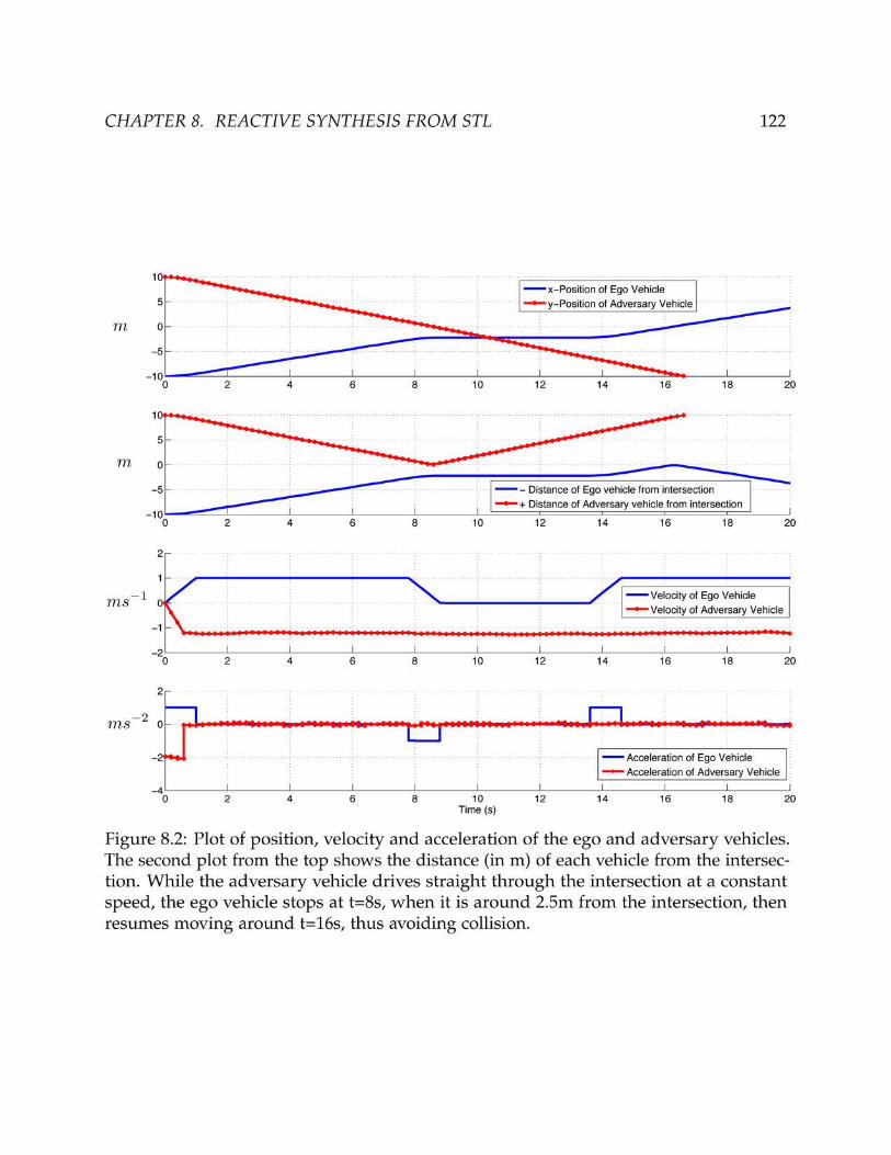

123
Chapter 9
Safe Control under Uncertainty
Achieving safe control under uncertain models for human-robot systems is challenging.For example, any safe control strategy for quadcopters need to incorporate predictive in-formation about wind gusts and any associated uncertainty in such predictions. Similarly,in the case of autonomous driving, the controller needs a probabilistic predictive modelabout the other vehicles on the road to avoid collisions. Without a model of uncertaintythat characterizes all possible outcomes, there is no hope in giving guarantees about thesafety of the synthesized controller.
The field of machine learning (ML) has a rich set of tools that can characterizeuncertainties. Specifically, Bayesian graphical models [85] have been popular in modelinguncertainties arising in scenarios common to robotics. For example, one of the commonstrategies is to build classifiers or predictors based on acquired sensor data. It is appealingto consider such predictors in achieving safe control of dynamical systems. However, itis almost impossible to guarantee a prediction system that works perfectly at all times.Consequently, we need to devise control methodologies aware of such limitations imposedby the ML systems. Specifically, we need to build a framework that is capable of achievingsafe control by being aware of when the prediction system would work or fail.
In this chapter, we propose a framework for achieving safe control, when machinelearning models are employed to make predictions based on sensed signals. The heartof our framework is the novel Probabilistic Signal Temporal Logic (PrSTL) that allows usto express safety constraints by considering the predictive models and their associateduncertainties. This logic allows specifications that embed Bayesian classification methodsvia probabilistic predicates that take random variables as parameters, thereby resulting ina powerful framework that can reason about safety under uncertainty. One of the mainadvantages of using Bayesian classification models is the fact that the predictions providedare full distributions associated with the quantity of interest as opposed to a pointestimate. For example, a classical machine learning method might just provide a valuefor wind speed; however, under the Bayesian paradigm we would be recovering an entireprobability distribution over all possible wind profiles. Finally, another distinguishingaspect of our framework is that these probabilistic predicates are adaptive: as the system

CHAPTER 9. SAFE CONTROL UNDER UNCERTAINTY 124
sees more and more data, the inferred distribution over the latent variables of interest canchange leading to change in the predicates themselves.
Previous efforts for achieving safe control either operate under deterministic envi-ronments or model uncertainty only as part of the dynamics of the system [72]. Theseapproaches lack clear connections to various sources of uncertainty present in the envi-ronment. Specifically, there is no clear understanding of how uncertainty arising due tosensing and classification could be incorporated while reasoning about safe controllers.
Over the years researchers have proposed different approaches for safe control ofdynamical systems. Designing controllers under reachability analysis and safe learningare well-studied methods that allow specifying safety and reachability properties, whilelearning the optimal strategy online [122, 121, 67, 13, 5]. However, finding the reachableset is computationally expensive, which makes these approaches impractical for mostinteresting tasks. Controller synthesis under temporal specifications such as LinearTemporal Logic (LTL) allows expressing interesting properties of the system and envi-ronment, e. g., safety, liveness, response, stability, and has shown promising results [139,97, 87, 184, 88, 140]. However, synthesis for LTL requires time and space discretization,which suffers from the curse of dimensionality. Also, while such approaches are effectiveat high level planning, they are unsuitable for lower level control of dynamical systems.Recently, synthesis for Signal Temporal Logic (STL), which allows real-valued, dense-timeproperties have been studied in receding horizon settings [148, 89, 65]. One downside ofspecifying properties in STL or LTL is that the properties of the system and environmenthave to be expressed deterministically. Full knowledge of the exact parameters andbounds of the specification is an unrealistic assumption for most robotics applications,where the system interacts with uncertain environments. Related to our work is theparadigm of Markov Logic Networks [150] that aim to induce probability distributionsover possible worlds by considering weighted logical formulae. However, it is not clearhow such networks can be used for controller synthesis. The proposed framework insteadconsiders formulae parameterized by random variables, thereby inducing probabilitydistribution over the set of possible formulae. Further, we show how such formalismcan be embedded in a receding horizon MPC for controller synthesis. In robust control,uncertainty is modeled as part of the dynamics, and the optimal strategy is found for theworst case disturbance, which can be a conservative assumption [96, 178]. More recently,the uncertainty is modeled in a chance constrained framework showing promising re-sults for urban autonomous driving [105, 176, 29, 36]. Considering uncertainties whilesatisfying temporal logic requirements has recently been explored for controller synthesisand verification [157, 168, 60, 61, 144, 83]. Leahy et al. maximize information gain ina distributed setting to reduce the uncertainty over belief of every state; however, theuncertainty is not considered as part of the specification [103]. To best of our knowledge,none of the previous studies consider scenarios, where the uncertainty and confidence inproperties are originated from sensors, predictors and classifiers, and are formalized aspart of the property.
In this chapter, we aim to alleviate these issues by defining a probabilistic logical

CHAPTER 9. SAFE CONTROL UNDER UNCERTAINTY 125
specification framework that has the capacity to reason about safe control strategiesby embedding various predictions and their associated uncertainty. Specifically, ourcontributions in this chapter are:
• Framework for safe control under uncertainty.
• Formally define PrSTL, a logic for expressing probabilistic properties that can embedBayesian graphical models.
• Solve a receding horizon control problem to satisfy PrSTL specifications usingMixed Integer SDPs.
• A toolbox implementing the framework and experiments in autonomous drivingand control of quadrotors.
9.1 Bayesian Classification to Model Uncertainty:
Probability theory provides a natural way to represent uncertainty in the environmentand recent advances in machine learning have relied on Bayesian methods to inferdistributions over latent phenomenon of interest [64, 85]. We focus on Bayesian classifiers,which unlike other optimization based methods, provide entire distributions over thepredictions. Such predictive distributions characterize the uncertainty present in thesystem and are crucial for achieving safe control. Formally, given a set of trainingpoints XL = x1, . . . , xn, with observations tL = t1, . . . , tn, where ti ∈ +1,−1, weare interested in finding a hyperplane w that separates the points belonging to the twoclasses according to sgn(wTx). Under the Bayesian paradigm, we look for the distribution:
p(w|XL, tL) = p(w) · p(tL|XL, w) =
p(w)∏i
p(ti|w, xi) = p(w)∏i
I [sgn(wTxi) = ti].(9.1)
The first line in the above equation stems from the Bayes rule, and the second line simplyexploits the fact that given the classifier w the labels for each of the points in the datasetare independent. The expression I[·] is an indicator function, which evaluates to 1, whenthe condition inside the brackets holds. Thus, equation (9.1) starts from a prior p(w) overthe classifiers and eventually by incorporating the training data points, infers a posteriordistribution over the set of all the classifiers that respect the observed labels and the points.Given these statistical dependencies among the various variables, Bayesian inferencetechniques [120, 21, 12] aim to infer p(w|XL, tL) as a Gaussian distribution N (w; w, Σ).Linear classification of a test data point wTx results in a Gaussian distribution of theprediction with the mean wTx and the variance xTΣx. Similarly, for the case of Bayesianlinear regression the same procedure can be followed, albeit with continuous targetvariables t ∈ R. These Bayesian linear classifiers and regressors are a fairly rich class of

CHAPTER 9. SAFE CONTROL UNDER UNCERTAINTY 126
models, and have similar or better representation capabilities as kernel machines [179]. Inthis chapter, we specifically aim to incorporate such rich family of classification modelsfor safe control.
9.2 Probabilistic Controller Synthesis Problem
We propose Probabilistic Signal Temporal Logic (PrSTL) that enables expression of un-certainty over the latent variables via probabilistic specifications. The key idea is toincorporate random variables in predicates, and then express temporal and Booleanoperations on such predicates. The proposed logic provides an expressive framework fordefining safety conditions under a wide variety of uncertainties, including ones that arisefrom application of machine learning classifiers.
The core ingredient in this chapter is the insight that when the uncertainty overthe random variable is reasoned out in a Bayesian framework, we can use the inferredprobability distributions to efficiently derive constraints from the PrSTL specifications. Weprovide a novel solution for synthesizing controllers for dynamical systems given differentPrSTL properties. An interesting aspect of this framework is that the PrSTL formulae canevolve at every step. For example, a classifier associated with the dynamical system cancontinue to learn with time, thereby changing the inferred probability distributions onthe latent random variables.
Probabilistic Signal Temporal Logic
PrSTL supports probabilistic temporal properties on real-valued, dense-time signals.Specifically, (ξ, t) |= ϕ denotes the signal ξ satisfies the PrSTL formula ϕ at time t. Weintroduce the notion of a probabilistic atomic predicate λǫt
αtof a PrSTL formula that is
parameterized with a time-varying random variable αt drawn from a distribution p(αt):
(ξ, t) |= λǫtαt⇐⇒ P(λαt(ξ(t)) < 0) > 1− ǫt. (9.2)
Similar to STL (see Chapter 2.3), with a slight abuse of notation, we let λǫtαt
denotethe probabilistic atomic predicate, and λαt be a function of the signal ξ(t). Here, P(·)represents the probability of the event, and 1− ǫt defines the tolerance level in satisfactionof the probabilistic properties. The parameter ǫt ∈ [0, 0.5] is a small time-varying positivenumber and represents the threshold on satisfaction probability of λαt(ξ(t)) < 0. Smallvalues of ǫt favors high tolerance satisfaction of formulas, which also facilitates solvingthe controller synthesis problem as discussed later in this section. A signal ξ(t) satisfiesthe PrSTL predicate λǫt
αtwith confidence 1− ǫt if and only if:
∫
αt
I[λαt(ξ(t)) < 0] p(αt) dαt > 1− ǫt. (9.3)

CHAPTER 9. SAFE CONTROL UNDER UNCERTAINTY 127
Here, I[·] is an indicator function, and the equation marginalizes out the random variableαt with the probability density p(αt). The truth value of the PrSTL predicate λǫt
αtis
equivalent to satisfaction of the probabilistic constraint in equation (9.2). Computingsuch integrals as in equation (9.3) for general distributions is computationally difficult;however, there are many parameterized distributions (e.g., Gaussian and other membersof the exponential family) for which there exists either a closed form solution or efficientnumerical procedures.
Note that λαt(ξ(t)) is a stochastic function of the signal ξ at time t and expresses amodel of the uncertainty in environment based on the observed signals. As the systemevolves and observes more data about the environment, the distribution over the randomvariable αt changes over time, thereby leading to an adaptive PrSTL predicate. ThePrSTL formula consists of Boolean and temporal operations over their predicates. Werecursively define the syntax of PrSTL as:
ϕ ::= λǫtαt| ¬λǫt
αt| ϕ ∧ ψ | ϕ ∨ ψ |G[a,b]ψ | ϕ U[a,b]ψ | F[a,b]ψ.
Here, ϕ is a PrSTL formula, which is built upon predicates λǫtαt
defined in equation (9.2),propositional formulae ϕ composed of the predicates and Boolean operators such as ∧(and), ¬ (negation), and temporal operators on ϕ such as G (globally), F (eventually) and U(until). Note, that in these operations the PrSTL predicates can have different probabilisticparameters, i. e., αt and ǫt. In addition, satisfaction of the PrSTL formulae for each of theBoolean and temporal operations based on the predicates is defined as:
(ξ, t) |= λǫtαt
⇔ P(λαt(ξ(t)) < 0) > 1− ǫt
(ξ, t) |= ¬λǫtαt
⇔ P(−λαt(ξ(t)) < 0) > 1− ǫt
(ξ, t) |= ϕ ∧ ψ ⇔ (ξ, t) |= ϕ ∧ (ξ, t) |= ψ(ξ, t) |= ϕ ∨ ψ ⇔ (ξ, t) |= ϕ ∨ (ξ, t) |= ψ(ξ, t) |= G[a,b]ϕ ⇔ ∀t′ ∈ [t + a, t + b], (ξ, t′) |= ϕ
(ξ, t) |= F[a,b]ϕ ⇔ ∃t′ ∈ [t + a, t + b], (ξ, t′) |= ϕ
(ξ, t) |= ϕ U[a,b] ψ ⇔ ∃t′ ∈ [t + a, t + b] s.t. (ξ, t′) |= ψ
∧∀t′′ ∈ [t, t′], (ξ, t′′) |= ϕ.
Remark 12. PrSTL does not follow the law of excluded middle, while it follows the law ofnoncontradiction. This means it will never be the case for a formula and its negation ¬, asdefined above, to both satisfy a specification at the same time. However, there exists situations,where they both can violate a specification.
Remark 13. The PrSTL framework reduces to STL, when the distribution p(αt) is a Diracdistribution. A Dirac or a point distribution over αt enforces λαt(ξ(t)) < 0 to be deterministicand equivalent to an STL predicate µ defined in Chapter 2.3.

CHAPTER 9. SAFE CONTROL UNDER UNCERTAINTY 128
Controller Synthesis for Probabilistic STL
We now formally define the controller synthesis problem in the MPC framework withPrSTL specifications.
Problem 9. Given a hybrid dynamical system as in equation (2.3), initial state x0, PrSTL for-mula ϕ, and cost function J(ξH) defined over a finite horizon trajectory ξH, find:
argminuH
J(ξH(x0, uH)) subject to ξH(x0, uH) |= ϕ. (9.4)
Problem (9) formulates a framework for finding a control strategy uH that optimizesa given cost function, and satisfies a PrSTL formula. Finding the best strategy for thisoptimization given only deterministic PrSTL formulae, where αt is drawn from a Diracdistribution is the same as solving a set of mixed integer linear constraints. We now showhow the optimization is solved for the general case of PrSTL. Specifically, we providefull solution for Gaussian distributions, where the optimization reduces to mixed integersemi-definite programs.
Mixed Integer Constraints
We first discuss how every PrSTL formula generates a set of integer constraints. Givena PrSTL formula, we introduce two integer variables for every time step t, p
ϕt and
qϕt ∈ 0, 1, which correspond to the truth value of the PrSTL formula and its negation
respectively. These variables enforce satisfaction of the formula ϕ as:
(pϕt = 1)→ (ξ, t) |= ϕ and (q
ϕt = 1)→ (ξ, t) |= ¬ϕ (9.5)
The formula ϕ holds true if pϕt = 1, and its negation ¬ϕ (defined in Section 9.2) holds true
if qϕt = 1. Due to the definition of negation, and Remark 12, these implications are only
one-way, i. e., there always exist a satisfiable solution when pϕt and q
ϕt are zero. Using both
integer variables, we define the constraints required for logical and temporal operationsof PrSTL on p
ϕt and q
ϕt . It is important to note that p
ϕt and q
ϕt are not functions of the
truth value of the formula ϕ, so their values are not meant to be uniquely determined.Instead, the integer variables enforce the truth value of the formula ϕ. We refer to themas truth value enforcers:
• Negation (ϕ = ¬ψ) : pϕt ≤ q
ψt and q
ϕt ≤ p
ψt
• Conjunction (ϕ = ∧Ni=1ψi) : p
ϕt ≤ p
ψit and q
ϕt ≤ ∑
Ni=1 q
ψit
• Disjunction (ϕ = ∨Ni=1ψi) : ϕ = ¬ ∧N
i=1 ¬ψi
• Globally (ϕ = G[a,b]ψ) : pϕt ≤ p
ψt′ ∀t′ ∈ [t + a, min(t + b, H−1)],
qϕt ≤ ∑
t+bt′=t+a q
ψt′ (Only for t < H − b).

CHAPTER 9. SAFE CONTROL UNDER UNCERTAINTY 129
• Eventually (ϕ = F[a,b]ψ) : ϕ = ¬G[a,b]¬ψ.
• Unbounded Until (ϕ = ψ1 U[0,∞)ψ2) :∨H−1
t=0
(
(G[0,t]ψ1) ∧ (G[t,t]ψ2))
∨G[0,H−1]ψ1
• Bounded Until (ϕ = ψ1 U[a,b]ψ2) : ϕ = G[0,a]ψ1 ∧ F[a,b]ψ2 ∧G[a,a](ψ1U[0,∞)ψ2)
Here, we have shown how pϕt and q
ϕt are defined for every logical property such
as negation, conjunction, and disjunction, and every temporal property such as globally,eventually, and until. We use U to refer to unbounded until with infinite time interval,and U for bounded until.
While synthesizing controllers for PrSTL formulae in an MPC scheme, we sometimesare required to evaluate satisfaction of the formula outside of the horizon range. Forinstance, a property G[a,b]ϕ might need to be evaluated beyond H for some t′ ∈ [t + a, t +
b]. In such cases, our proposal is to act optimistically, i. e., we assume the formula holdstrue for the time steps outside the horizon of globally operator, and similarly assume theformula does not hold true for the negation of the globally operator. This optimism isevident in formulating the truth value enforcers of the globally operator, and based onthat, it is specified for other temporal properties. With the recursive definition of PrSTL,and the above encoding, the truth value enforcers of every PrSTL formula is definedusing a set of integer inequalities involving a composition of the truth value enforcers ofthe inner predicates.
Satisfaction of PrSTL predicates
We have defined the PrSTL predicate λǫtαt
for a general function, λαt(ξ(t)) of the signalξ at time t. This function allows a random variable αt ∼ p(αt) to be drawn from anydistribution at every time step. The general problem of controller synthesis satisfying thePrSTL predicates is computationally difficult since the evaluation of the predicates boilsdown to computing the integration in equation (9.3). Consequently, to solve the problemin equation (9.4), we need to enforce a structure on the predicates of ϕ. In this section, weexplore the linear-Gaussian structure of the predicates that appears in many real-worldscenarios, and show how it translates to Mixed Integer SDPs. Formally, if ϕ = λǫt
αtis only
a single predicate, the optimization in equation (9.4) will reduce to:
argminuH
J(ξH(x0, uH))
subject to (ξ, t) |= λǫtαt
∀t ∈ 0, . . . , H−1.(9.6)
This optimization translates to a chance constrained problem [25, 31, 175, 105, 29] at everytime step of the horizon, based on the definition of PrSTL predicates in equation (9.2):
argminuH
J(ξH(x0, uH))
subject to P(λαt(ξ(t)) < 0) > 1− ǫt
∀t ∈ 0, . . . , H−1.(9.7)

CHAPTER 9. SAFE CONTROL UNDER UNCERTAINTY 130
An important challenge with such chance constrained optimization is there are noguarantees that equation (9.7) is convex. The convexity of the problem depends on thestructure of the function λαt , and the distribution p(αt). It turns out that the problemtakes a simple convex form when λαt is linear-Gaussian, i. e., the random variable αt
comes from a Gaussian distribution and the function itself is linear in αt:
λαt(ξ(t)) = αt⊤ξx(t) = αt
⊤xt, αt ∼ N (µt, Σt). (9.8)
It is easy to show that for this structure of λαt , i.e., a weighted sum of the states withGaussian weights αt, the chance constrained optimization in equation (9.7) is convex [171,91]. Specifically, the optimization problem can be transformed to a second-order coneprogram (SOCP). First, consider a normally distributed random variable ν ∼ N (0, 1),
and its cumulative distribution function (CDF) Φ =∫ z−∞
1√2π
e−t2
2 dt. Then, the chance
constrained optimization reduces to SOCP:
P(λαt(ξ(t)) < 0) > 1− ǫt ⇔ P(α⊤t xt< 0) > 1− ǫt ⇔
P(ν <−µ⊤t xt
(xt)⊤Σtxt) > 1− ǫt ⇔
∫
−µ⊤t xt
(xt)⊤Σtxt
−∞
1√2π
e−t2
2 dt > 1− ǫt
⇔ Φ(µ⊤t xt
(xt)⊤Σtxt) < ǫt ⇔ µ⊤t xt −Φ−1(ǫt)||Σ1/2
t xt||2 < 0.
In this formulation, µ⊤t xt is the linear term, where µt is the mean of the random variable
αt at every time step, and ||Σ1/2t xt||2 is the l2-norm representing a quadratic term, where
Σt is the variance of αt. This quadratic term is scaled by Φ−1(ǫt), the inverse of theNormal CDF function, which is negative for small values of ǫt ≤ 0.5. Thus, every chanceconstraint can be reformulated as a SOCP, and as a result with a convex cost functionJ(ξH), we can efficiently solve the following convex optimization for every predicate ofPrSTL:
minimizeuH
J(ξH(x0, uH))
subject to µ⊤t xt −Φ−1(ǫt)||Σ1/2t xt||2 < 0
∀t ∈ 0, . . . , H − 1.(9.9)
Assuming a linear-Gaussian form of the function, we generate the SOCP above, andtranslate it to a semi-definite program (SDP) by introducing auxiliary variables [31]. Weuse this SDP that solves the problem in equation (9.6) with a single constraint ϕ = λǫt
αtas a
building block, and use it multiple times to handle complex PrSTL formulae. Specifically,any PrSTL formula can be decomposed to its predicates by recursively introducing integervariables that correspond to the truth value enforcers of the formula at every step asdiscussed in Section 9.2.
We would like to point out that assuming linear-Gaussian form of λαt is not toorestrictive. The linear-Gaussian form subsumes the case of Bayesian linear classifiers,

CHAPTER 9. SAFE CONTROL UNDER UNCERTAINTY 131
and consequently the framework can be applied to a wide variety of scenarios wherea classification or regression function needs to estimate quantities of interest that arecritical for safety. Furthermore, the framework is applicable to all random variables whosedistributions exhibit unimodal behavior and aligned with the large law of numbers. Fornon-Gaussian random variables, there are many approximate inference procedures thateffectively estimate the distributions as Gaussian.
Convex Subset of PrSTL
As discussed in Section 9.2, at the predicate level of ϕ, we create a chance constrainedproblem for predicates λǫt
αt. These predicates of the PrSTL formulae can be reformulated
as a semi-definite program, where the predicates are over intersections of cone of positivedefinite matrices with affine spaces. Semi-definite programs are special cases of convexoptimization; consequently, solving Problem 9, only for PrSTL predicates is a convexoptimization problem. Note that in Section 9.2 we introduced integer variables fortemporal and Boolean operators of the PrSTL formula. Construction of such integervariables increases the complexity of Problem 9, and results in a mixed integer semi-definite program (MISDP). However, we are not always required to create integer variables.Therefore, we define Convex PrSTL as a subset of PrSTL formulae that can be solvedwithout constructing integer variables.
Definition 2. Convex PrSTL is a subset of PrSTL such that it is recursively defined over thepredicates by applying Boolean conjunctions, and the globally temporal operator. Satisfaction ofa convex PrSTL formulae is defined as:
(ξ, t) |= λǫtαt
⇔ P(λαt(ξ(t)) < 0) > 1− ǫt
(ξ, t) |= ϕ ∧ ψ ⇔ (ξ, t) |= ϕ ∧ (ξ, t) |= ψ(ξ, t) |= G[a,b]ϕ ⇔ ∀t′ ∈ [t + a, t + b], (ξ, t′) |= ϕ
Theorem 11. Given a convex PrSTL formula ϕ, a hybrid dynamical system as defined in equa-tion (2.3), and an initial state x0; the controller synthesis problem (Problem 9) is convex under aconvex cost function J.
Proof. We have shown that the predicates of ϕ, i. e., λǫtαt
create a set of convex constraints.The Boolean conjunction of convex programs are also convex; therefore, ϕ ∧ ψ resultin convex constraints. In addition, the globally operator is defined as a set of finite
conjunctions over its time interval: G[a,b]ϕ =∧b
t=a ϕt. Thus, the globally operator retainsthe convexity property of the constraints. Consequently, Problem 9, with a convex PrSTLconstraint ϕ is a convex program.
Theorem 11 allows us to efficiently reduce the number of integer variables required forsolving Problem 9. We only introduce integer variables when disjunctions, eventually, oruntil operators appear in the PrSTL constraints. Even when a formula is not completely

CHAPTER 9. SAFE CONTROL UNDER UNCERTAINTY 132
Algorithm 6 Controller Synthesis with PrSTL Formulae
1: Inputs: f , x0, H, τ, J, ϕ2: Let τ = [t1, t2] is the time interval of interest.3: past← Initialize(t1)4: for t = t1: dt: t2 do5: flin = linearize( f , ξ(t))6: αt ← Update Distributions(αt−dt, sense(ξx(t)))7: ϕ← ϕ(αt, ǫt)8: CPrSTL = MISDP(ϕ)9: C = CPrSTL ∧ flin ∧ [ ξ(max(t1, t− H) · · · t− dt) = past ]
10: uH = optimize(
J(ξH), C)
11: xt+1 = f (xt, ut)12: past← [past ξ(t)]13: Drop the first element of past if len(past) >
Hdt
14: end for
part of the Convex PrSTL, integer variables are introduced only for the non-convexsegments.
We show our complete method of controlling dynamical systems in uncertain envi-ronments in Algorithm 6. At the first time step t1, we run an open-loop control algorithmto populate past in line 2. We then run the closed-loop algorithm, finding the optimalstrategy at every time step of the time interval τ = [t1, t2]. In the closed-loop algorithm,we linearize the dynamics at the current local state and time in line 4, and then updatethe distributions over the random variables in the PrSTL formula based on new sensordata in line 5. Then, we update the PrSTL formulae, based on the updated distributions.If there are any other dynamic parameters that change at every time step, they can alsobe updated in line 6. In line 7, we generate the mixed integer constraints in CPrSTL, andpopulate C with all the constraints including the PrSTL constraints, linearized dynamics,and enforcing to keep the past horizon’s trajectory. Note that we do not construct integervariables if the formula is Convex PrSTL. Then, we call the finite horizon optimizationalgorithm under the cost function J(ξH), and the constraints C in line 9, which provides alength H strategy uH. We advance the state with the first element of uH, and update theprevious horizon’s history in past. The size of this problem does not grow, and keepingthe past horizon history is crucial in satisfaction of fairness properties, e. g., enforcinga signal to oscillate. We continue running this loop and synthesizing controllers for alltimes in interval τ. Algorithm 6 solves MISDP problems, which is NP-hard. However,the actual runtime depends on the size of the MISDP, which is linear in the number ofpredicates and operators in the PrSTL specification. For convex PrSTL, the complexity isthe same as an SDP, which is cubic in the number of constraints [104].


CHAPTER 9. SAFE CONTROL UNDER UNCERTAINTY 134
Here, we penalize the l2-norm of the Euler angles, which enforces a resulting smoothtrajectory. Besides initializing the state and control input at zero, we bound the controlinputs via the following deterministic PrSTL formulae (here only shown for roll, similarform follows for pitch and thrust):
ϕroll = G[0,∞)(||u1|| ≤ 0.3) Bound on Roll Input
In Figure 9.1, the gray surface is a ceiling that the quadrotor should not collide with as itis taking off and landing at the final position. However, the quadrotor does not have afull knowledge of where the ceiling is exactly located. We define a sensing mechanism forthe quadrotor, which consists of a meshgrid of points around the body of the quadrotor.As the system moves in the space, a Bayesian binary classifier is updated by providing asingle label −1 (no obstacles present) or 1 (obstacle present) for each of the sensed points.
The Bayesian classifier is the same as the Gaussian Process based method describedin Section 9.1 and has the linear-Gaussian form. Applying this classifier results in aGaussian distribution for every point in the 3D-space. We define our classifier withconfidence 1− ǫt = 0.95, as the stochastic function λ0.05
αt(ξ(t)) = α⊤t [x
t yt zt]. Here, xt,
yt, zt are the coordinates of the sensing points, and αt ∼ N (µt, Σt) is the Gaussian weightinferred over time using the sensed data. We define a time-varying probabilistic constraintthat needs to be held at every step as its value changes over time. Our constraint specifiesthat given a classifier based on the sensing points parameterized by αt, we would enforcethe quadrotor to stay within a safe region (defined by the classifier) with probability1− ǫt at all times. Thus the probabilistic formula is:
ϕclassifier = G[0.1,∞)
(
P(α⊤t [xt yt zt] < 0) > 0.95
)
.
We enforce this probabilistic predicate at t ∈ [0.1, ∞), which verifies the property startingfrom a small time after the initial state, so the quadrotor has gathered some sensor data.In Figure 9.1, the pink surface represents the second order cone created based on ϕclassifier,at every step characterized by:
µ⊤t[
xt yt zt]
−Φ−1(0.05)||Σ1/2t
[
xt yt zt]
||2 < 0.
Note that the surface shown in Figure 9.1, at the initial time step is not an accurateestimate of where the ceiling is, and it is based on a distribution learned from the initialvalues of the sensors. Thus, if the quadrotor was supposed to follow this estimate withoutupdating, it would have collided with the ceiling. In Figure 9.2, the blue path representsthe trajectory the quadrotor has already taken, and the dotted green line is the futureplanned trajectory based on the current state of the classifier. The dotted green trajectoryat the initial state goes through the ceiling since the belief of the location of the ceilingis incorrect; however, the trajectory is modified at every step as the Bayesian inferenceupdates the distribution over the classifier. As shown in Figure 9.2, the pink surfacechanges at every time step, and the learned parameters µt, and Σt are updated, so the

CHAPTER 9. SAFE CONTROL UNDER UNCERTAINTY 135
quadrotor safely reaches the final position. We solve the optimization using our toolbox,with dt = 0.03, and horizon of H = 20. These choices describe a common setting forsolving MPC problems. We emphasize that some of the constraints are time-varying,and we need to update them at every step of the optimization. We similarly updatethe dynamics at every step, since we locally linearize the dynamics around the currentposition of the quadrotor.
Control under Battery Constraints
Next we demonstrate a scenario that addresses safety, when there is uncertainty aroundthe battery level. The battery level is a stochastic variable due to uncertain environmentand usage factors, such as radio communications, etc. Our goal is to derive a safestrategy that considers such stochasticity. We start by augmenting the logarithm of batterylevel (bt) to the state space of the system discussed above. Thus, the quadrotor is a 13dimensional system, where the first 12 states follow the same order and system dynamicsas before and xt(13) = log(bt). In our model, the state of log(bt) evolves with the negative
thrust value:d log(bt)
dt = −|u4|. We enforce the same constraints to bound the control asearlier, and the objective of the quadrotor is to start from the origin and reach the topdiagonal corner of the space with coordinates (1, 1,−0.9) smoothly.
We then consider adding a safety invariant that would limit high altitude flights if thebattery level is low. The following formulae describe these constraints:
• φ := F[0,0.3](zt ≤ −0.1) encodes that eventually in the next 0.3 s, the quadrotor will
fly above a threshold level of −0.1 m.
• ψ := P(log(bt) + N (0, tσ2) ≥ bmin) ≥ 1 − ǫt represents the constraint that thequadrotor has to be confident that the logarithm of its battery state perturbed by atime-varying variance is above bmin.
Now, we can combine the two formulae to specify the condition that the quadrotor needsto fly low if the battery state is low:
ϕbattery := G[0,∞)
(
φ→ ψ)
. (9.10)
The → in the formula ϕbattery is the implication relation, and intuitively states thatanytime the quadrotor flies above the threshold then it means that there is sufficientbattery reserve.
We synthesize a controller for the specifications with ǫt = 0.2. The trajectory of thequadrotor is shown in Figure 9.3. Figure 9.3a corresponds to σ = 0, i. e., the battery statechanges deterministically, and Figure 9.3b, corresponds to σ = 10, when the quadrotor ismore cautious about the state of the battery. Note the safe trajectory does not pass the−0.1 m height level whenever the confidence in the battery level is low.
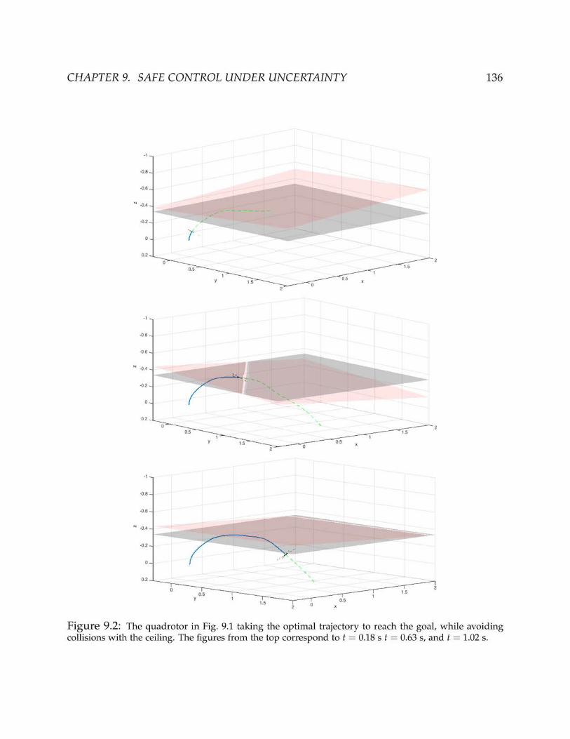
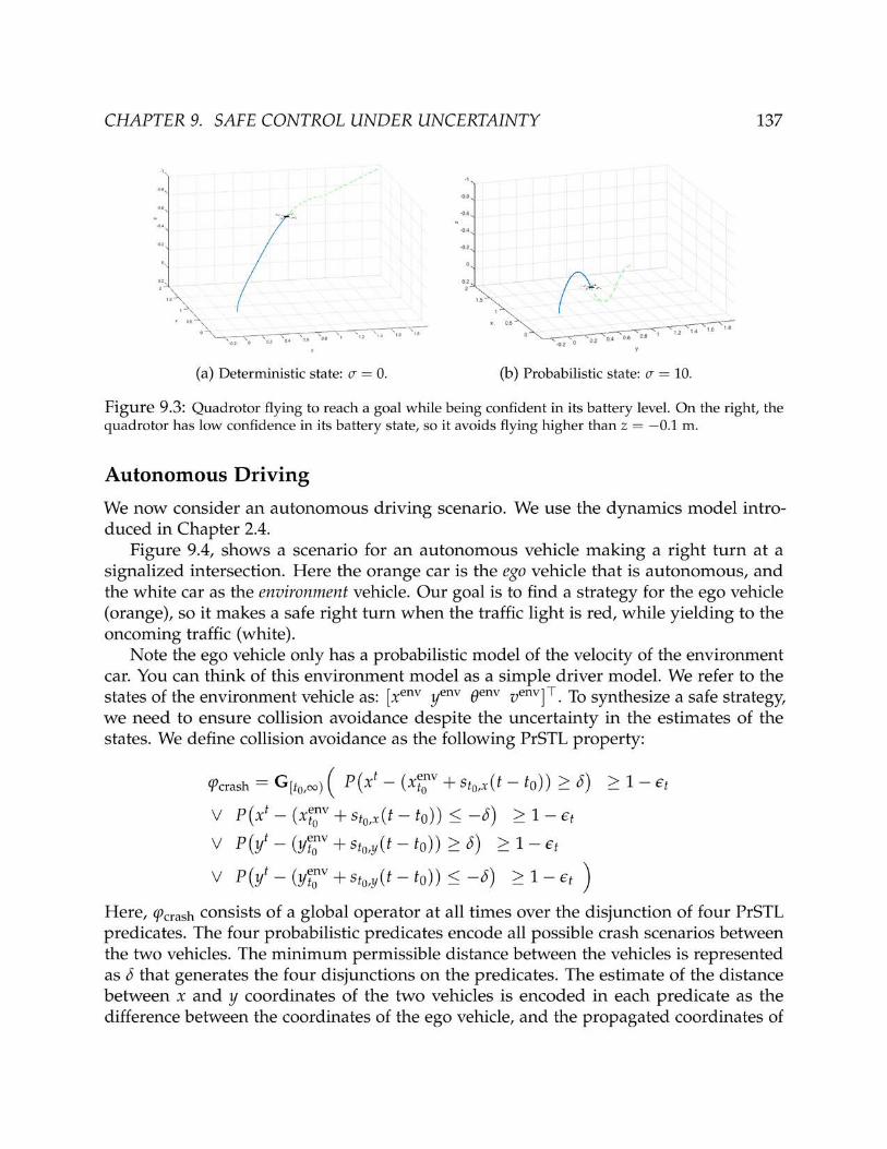


CHAPTER 9. SAFE CONTROL UNDER UNCERTAINTY 139
9.4 Chapter Summary
We presented a framework to achieve safe control under uncertainty. The key contri-butions include defining PrSTL, a logic for expressing probabilistic properties that canembed Bayesian graphical models. We also show how to synthesize receding horizoncontrollers under PrSTL specifications that express Bayesian linear classifiers. Further,the resulting logic adapts as more data is observed with the evolution of the system.We demonstrate the approach by synthesizing safe strategies for a quadrotor and anautonomous vehicle traveling in uncertain environments.
The approach extends easily to distributions other than Gaussians via Bayesianapproximate inference techniques [120, 21] that can project distributions to the Gaussiandensities. Future work includes extending controller synthesis for arbitrary distributionsvia sampling based approaches; we are also exploring using the proposed framework forcomplex robotic tasks that need to invoke higher level planning algorithms. We furtherplan to combine controller synthesis from PrSTL with sampling based task planners thatcan be guaranteed to be safe under probabilistic specifications.

140
Chapter 10
Diagnosis and Repair for Synthesis fromSignal Temporal Logic
A major challenge to the adoption of synthesis from temporal logic in practice is thedifficulty of writing formal specifications – writing temporal logic specifications is noteasy and is error-prone, even for experts. Specifications that are poorly stated, incomplete,or inconsistent can produce synthesis problems that are unrealizable (no controller existsfor the provided specification), intractable (synthesis is computationally too hard), orlead to solutions that fail to capture the designer’s intent. In this chapter, we present analgorithmic approach to reduce the specification burden for controller synthesis fromtemporal logic specifications, focusing on the case where the original specification isunrealizable.
Logical specifications can be provided in multiple ways. One approach is to providemonolithic specifications, combining within a single formula constraints on the environ-ment with desired properties of the system under control. In many cases, a systemspecification can be conveniently provided as a contract, to distinguish the responsibilitiesof the system under control (guarantees) from the assumptions on the external, possiblyadversarial environment [135, 136]. In such a scenario, an unrealizable specification canbe made realizable by either “weakening” the guarantees or “tightening” the assumptions. Infact, when a specification is unrealizable, it could be either because the environmentassumptions are too weak, or the requirements are too strong, or a combination ofboth. Finding the “problem” with the specification manually can be a tedious and time-consuming process, nullifying the benefits of automatic synthesis. Further, in the reactivesetting, when the environment is adversarial, finding the right assumptions a priori canbe difficult. Thus, given an unrealizable logical specification, there is a need for tools thatlocalize the cause of unrealizability to (hopefully small) parts of the formula, and providesuggestions for repairing the formula in an “optimal” manner.
The problem of diagnosing and repairing formal requirements has received its shareof attention in the formal methods community. Ferrère et al. perform diagnosis on faultyexecutions of systems with specifications expressed in Linear Temporal Logic (LTL) and

CHAPTER 10. DIAGNOSIS AND REPAIR 141
Metric Temporal Logic (MTL) [59]. They identify the cause of unsatisfiability of theseproperties in the form of prime implicants, which are conjunctions of literals, and mapthe failure of a specification to the failure of these prime implicants. Similar syntax-tree based definitions of unsatisfiable cores for LTL were presented by Schuppan [162].In the context of synthesis from LTL specifications, Raman et al. [145] address theproblem of categorizing the causes of unrealizability, and how to detect them in high-levelrobot control specifications. The use of counter-strategies to debug unrealizable coresin a set of specifications or derive new environment assumptions for synthesis has alsobeen explored [109, 95, 9, 110]. Our approach, based on exploiting information alreadyavailable from off-the-shelf optimization solvers, is similar to the one adopted by Nuzzo etal. [134] to extract unsatisfiable cores for Satisfiability Modulo Theories (SMT) solving.
In this chapter, we address the problem of diagnosing and repairing specifications for-malized in Signal Temporal Logic (STL). Our work is conducted in the setting of automatedsynthesis from STL using optimization methods in a Model Predictive Control (MPC)framework similar to the previous chapters [147, 148]. In this approach to synthesis, boththe system dynamics and the STL requirements encoded as mixed integer constraintson variables modeling the dynamics of the system and its environment. Controllersynthesis is then formulated as an optimization problem to be solved subject to theseconstraints [147]. In the reactive setting, this approach proceeds by iteratively solving acombination of optimization problems using a Counterexample-Guided Inductive Synthesis(CEGIS) scheme (see Chapter 8) [148]. In this context, an unrealizable STL specifica-tion leads to an infeasible optimization problem. We leverage the ability of existingMixed Integer Linear Programming (MILP) solvers to localize the cause of infeasibility toso-called Irreducibly Inconsistent Systems (IIS). Our algorithms use the IIS to localize thecause of unrealizability to the relevant parts of the STL specification. Additionally, wegive a method for generating a minimal set of repairs to the STL specification such that,after applying those repairs, the resulting specification is realizable. The set of repairsis drawn from a suitably defined space that ensures that we rule out vacuous and otherunreasonable adjustments to the specification. Specifically, in this chapter, we focus onthe numerical parameters in a formula, since their specification is often the most tediousand error-prone part. Our algorithms are sound and complete, i. e., they provide a correctdiagnosis, and always terminate with a reasonable specification that is realizable usingthe chosen synthesis method, when such a repair exists in the space of possible repairs.Recall that Chapter 7 discussed the design of an intervention framework to systematicallytransfer control to the human while synthesizing control strategies from LTL. In a similarmanner, in this chapter our diagnosis and repair algorithms provide a way of detectingthe source of unrealizability in the reactive synthesis problem from STL (discussed inChapter 8). Likewise, this can then be used to design interventions in a shared controlframework for a human-robot system.
The problem of infeasibility in constrained predictive control schemes has also beenwidely addressed in the literature, e.g., by adopting robust MPC approaches, soft con-straints, and penalty functions [92, 163, 24]. Rather than tackling general infeasibility

CHAPTER 10. DIAGNOSIS AND REPAIR 142
issues in MPC, our focus is on providing tools to help debug the controller specificationat design time. However, the deployment of robust or soft-constrained MPC approachescan also benefit from our techniques. Our use of MILP does not restrict our method tolinear dynamical systems; indeed, we can handle constrained linear and piecewise affinesystems, Mixed Logical Dynamical (MLD) systems [23], and certain differentially flatsystems.
10.1 Mixed Integer Linear Program Formulation
We described the approach of using Model Predictive Control in Chapter 2.1. When f ,the dynamics of the system, as defined in (2.3), is nonlinear, we assume optimization isperformed at each MPC step after locally linearizing the system dynamics. For example, attime t = k, the linearized dynamics around the current state and time are used to computean optimal strategy uH
∗ over the time interval [k, k + H − 1]. Only the first component ofuH∗ is, however, applied to the system, while a similar optimization problem is solved at
time k + 1 to compute a new optimal control sequence along the interval [k + 1, k + H]for the model linearized around t = k + 1. While the global optimality of MPC is notguaranteed, the technique is frequently used and performs well in practice.
In this chapter, we use STL to express temporal constraints on the environment andsystem runs for MPC. We then translate a STL specification into a set of mixed integerlinear constraints, as further detailed below [147, 148]. Given a formula ϕ to be satisfiedover a finite horizon H, the associated optimization problem has the form:
minimizeuH
J(ξ(x0, uH))
subject to ξ(x0, uH) |= ϕ,(10.1)
which extracts a control strategy uH that minimizes the cost function J(ξ) over thefinite-horizon trajectory ξ, while satisfying the STL formula ϕ at time step 0. In a closed-loop setting, we compute a fresh uH at every time step i ∈ N, replacing x0 with xi
in (10.1) [147, 148].While equation (10.1) applies to systems without uncontrolled inputs, a more general
formulation can be provided to account for an uncontrolled disturbance input wH thatcan act, in general, adversarially as discussed in Chapter 8. To provide this formulation,we assume that the specification is given in the form of a STL assume-guarantee (A/G)contract [135, 136] C = (V, ϕe, ϕ ≡ ϕe → ϕs), where V is the set of variables, ϕe capturesthe assumptions (admitted behaviors) over the (uncontrolled) environment inputs w,and ϕs describes the guarantees (promised behaviors) over all the system variables. Agame-theoretic formulation of the controller synthesis problem can then be represented

CHAPTER 10. DIAGNOSIS AND REPAIR 143
as a minimax optimization problem:
minimizeuH
maximizewH∈W e
J(ξ(x0, uH, wH))
subject to ∀wH ∈ W e ξ(x0, uH, wH) |= ϕ,(10.2)
where we aim to find a strategy uH that minimizes the worst case cost J(ξ) overthe finite horizon trajectory, under the assumption that the disturbance signal wH actsadversarially. We use W e in (10.2) to denote the set of disturbances that satisfy theenvironment specification ϕe, i.e.,W e = w ∈ WH|w |= ϕe.
To solve the control problems in (10.1) and (10.2) the STL formula ϕ can be translatedinto a set of mixed integer constraints, thus reducing the optimization problem to a MixedInteger Program (MIP), as long as the system dynamics can also be translated into mixedinteger constraints. Specifically, in this chapter similar to Chapter 8, we consider controlproblems that can be encoded as Mixed Integer Linear Programs (MILP).
The MILP constraints are constructed recursively on the structure of the STL specifica-tion as in [147, 148], and express the robust satisfaction value of the formula. A first setof variables and constraints capture the robust satisfaction of the atomic predicates ofthe formula. To generate the remaining constraints, we traverse the parse tree of ϕ fromthe leaves (associated with the atomic predicates) to the root node (corresponding to therobustness satisfaction value of the overall formula ρϕ), adding variables and constraintsthat obey the quantitative semantics discussed in Chapter 2.3.
Recall from Chapter 2.3 that the robustness value of subformulae with temporal andBoolean operators is expressed as the min or max of the robustness values of the operandsover time. We discuss here the encoding of the min operator as an example. To encodep = min(ρϕ1 , . . . , ρϕn), we introduce Boolean variables zϕi for i ∈ 1, . . . , n and MILPconstraints:
p ≤ ρϕi , ∑i=1...n
zϕi ≥ 1
ρϕi − (1− zϕi)M ≤ p ≤ ρϕi + (1− zϕi)M(10.3)
where M is a constant selected to be much larger than |ρϕi | for all i, and i ∈ 1, . . . , n.The above constraints ensure that zϕi = 1 and p = ρϕi only if ρϕi is the minimum over alli. For max, we replace ≤ by ≥ in the first constraint of (10.3). Finally, we choose ρϕ asthe cost function of the resulting MILP, meaning that our controllers aim at maximizingthe robustness of satisfaction of the specification. Note that the robustness function isanalogous to the robot reward function RR discussed in Part I; both encode a quantitativemeasure for satisfaction of the desired properties, and both are optimized to find thedesirable controllers for the robot.
We solve the resulting MILP with an off-the-shelf solver. If the receding horizonscheme is feasible, then the controller synthesis problem is realizable, i.e., the algorithmreturns a controller that satisfies the specification and optimizes the objective. However,if the MILP is infeasible, the synthesis problem is unrealizable. In this case, the failure to


CHAPTER 10. DIAGNOSIS AND REPAIR 145
using the formula ϕ := ϕ1 ∧ ϕ2, where ϕ1 and ϕ2 are defined as follows:
ϕ1 = G[0,∞)¬(
(−0.5 ≤ yegot ≤ 0.5) ∧ (−0.5 ≤ xadv
t ≤ 0.5))
,
ϕ2 = G[0,∞)
(
1.5 ≤ aegot ≤ 2.5
)
.(10.4)
We prescribe bounds on the system acceleration, and state that both cars should never be confinedtogether within a box of width 1 around the intersection (0, 0) to avoid a collision.
Example 3 (Non-adversarial Race). We discuss a race scenario, in which the ego vehicle mustincrease its velocity to exceed 0.5 whenever the adversary’s initial velocity exceeds 0.5. We thenformalize our requirement as a contract (ψe, ψe → ψs), where ψe are the assumptions made onthe environment and ψs are the guarantees of the system provided the environment satisfies theassumptions. Specifically:
ψe = (vadv0 ≥ 0.5),
ψs = G[0,∞)(−1 ≤ aegot ≤ 1) ∧G[0.2,∞)(v
egot ≥ 0.5).
(10.5)
The initial velocities are vadv0 = 0.55 and v
ego0 = 0, while the environment vehicle’s acceleration
is aadvt = 1 at all times. We also require the acceleration to be bounded by 1.
Example 4 (Adversarial Race). We discuss another race scenario, in which the environmentvehicle acceleration aadv
t is no longer fixed, but can vary up to a maximum value of 2. Initially,
vadv0 = 0 and v
ego0 = 0 hold. Under these assumptions, we would like to guarantee that the
velocity of the ego vehicle exceeds 0.5 if the speed of the adversary vehicle exceeds 0.5, whilemaintaining an acceleration in the [−1, 1] range. Altogether, we capture the requirements abovevia a contract (φw, φw → φs), where:
φw = G[0,∞)
(
0 ≤ aadvt ≤ 2
)
,
φs = G[0,∞)
(
(vadvt > 0.5)→ (v
egot > 0.5)
)
∧(
|aegot | ≤ 1
)
.(10.6)
10.3 Diagnosis and Repair Problem
In this section, we define the problems of specification diagnosis and repair in the contextof controller synthesis from STL. We assume that the discrete-time system dynamics fd,the initial state x0, the STL specification ϕ, and a cost function J are given. The controllersynthesis problem, denoted P = ( fd, x0, ϕ, J), is to solve (10.1) (when ϕ is a monolithicspecification of the desired system behavior) or (10.2) (when ϕ represents a contractbetween the system and the environment).
If synthesis fails, the diagnosis problem is, intuitively, to return an explanation in theform of a subset of the original problem constraints that are already infeasible when takenalone. The repair problem is to return a “minimal” set of changes to the specification

CHAPTER 10. DIAGNOSIS AND REPAIR 146
that would render the resulting controller synthesis problem feasible. To diagnose andrepair a STL formula, we focus on its sets of atomic predicates and time intervals of thetemporal operators. We then start by providing a definition of the support of its atomicpredicates, i.e., the set of times at which the value of a predicate affects satisfiability ofthe formula, and define the set of allowed repairs.
Definition 3 (Support). The support of a predicate µ in a STL formula ϕ is the set of times tsuch that µ(ξ(t)) appears in ϕ.
For example, given ϕ = G[6,10](xt> 0.2), the support of predicate µ = (xt
> 0.2) is
the time interval [6, 10]. We can compute the support of each predicate in ϕ by traversingthe parse tree of the formula from the root node to the leaves, which are associated withthe atomic predicates. The support of the root of the formula is 0 by definition. Whileparsing ϕ, new nodes are created and associated with the Boolean and temporal operatorsin the formula. Let κ and δ be the subsets of nodes associated with the Boolean andbounded temporal operators, respectively, where δ = δG ∪ δF ∪ δU. The support of thepredicates can then be computed by recursively applying the following rule for each nodei in the parse tree:
σi =
σr if r ∈ κ
σr + Ir if r ∈ δG ∪ δF
[σlbr , σub
r + Iubr ] if r ∈ δU,
(10.7)
where r is the parent of i, σr is the support of r, and Ii is the interval associated with iwhen i corresponds to a temporal operator. We denote as I1 + I2 the Minkowski sum ofthe sets I1 and I2, and as I lb and Iub, respectively, the lower and upped bounds of intervalI.
Definition 4 (Allowed Repairs). Let Φ denote the set of all possible STL formulae. A repairaction is a relation γ : Φ→ Φ consisting of the union of the following:
• A predicate repair returns the original formula after modifying one of its atomic predicatesµ to µ∗. We denote this sort of repair by ϕ[µ 7→ µ∗] ∈ γ(ϕ);
• A time interval repair returns the original formula after replacing the interval of a tem-poral operator. This is denoted ϕ[∆[a,b] 7→ ∆[a∗,b∗]] ∈ γ(ϕ) where ∆ ∈ G, F, U.
Repair actions can be composed to get a sequence of repairs Γ = γn(γn−1(. . . (γ1(ϕ)) . . . )).Given a STL formula ϕ, we denote as REPAIR(ϕ) the set of all possible formulae obtainedthrough compositions of allowed repair actions on ϕ. Moreover, given a set of atomicpredicates D and a set of time intervals T , we use REPAIRT ,D(ϕ) ⊆ REPAIR(ϕ) to denotethe set of repair actions that act only on predicates in D or time intervals in T . We arenow ready to provide the formulation of the problems addressed in the chapter, both interms of diagnosis and repair of a monolithic specification ϕ (general diagnosis and repair)and an A/G contract (ϕe, ϕe → ϕs) (contract diagnosis and repair).

CHAPTER 10. DIAGNOSIS AND REPAIR 147
Problem 10 (General Diagnosis and Repair). Given a controller synthesis problem P =( fd, x0, ϕ, J) such that (10.1) is infeasible, find:
• A set of atomic predicates D = µ1, . . . , µd or time intervals T = τ1, . . . , τd of theoriginal formula ϕ,
• ϕ′ ∈ REPAIRT ,D(ϕ),
such that P ′ = ( fd, x0, ϕ′, J) is feasible, and the following minimality conditions hold:
• (predicate minimality) if ϕ′ is obtained by predicate repair1, si = µ∗i − µi for i ∈1, . . . , d, sD = (s1, . . . , sd), and || · || is a norm on Rd, then
∄ (D′, sD′) s.t. ||sD′ || ≤ ||sD|| (10.8)
and P ′′ = ( fd, x0, ϕ′′, J) is feasible, with ϕ′′ ∈ REPAIRD′(ϕ).
• (time interval minimality) if ϕ′ is obtained by time interval repair, T ∗ = τ∗1 , . . . , τ∗l are the non-empty repaired intervals, and ||τ|| is the length of interval τ:
∄ T ′ = τ′1, . . . , τ′l , s.t. ∃i ∈ 1, . . . , l, ||τ∗i || ≤ ||τ′i || (10.9)
and P ′′ = ( fd, x0, ϕ′′, J) is feasible, with ϕ′′ ∈ REPAIRT ′(ϕ).
Problem 11 (Contract Diagnosis and Repair). Given a controller synthesis problem P =( fd, x0, ϕ ≡ ϕe → ϕs, J) such that (10.2) is infeasible, find:
• Sets of atomic predicates De = µe1, . . . , µe
d, Ds = µs1, . . . , µs
d or sets of time intervals
Te = τe1 , . . . , τe
l ,Ts = τs1 , . . . , τs
l, respectively, of the original formulas ϕe and ϕs,
• ϕ′e ∈ REPAIRTe,De(ϕe), ϕ′s ∈ REPAIRTs,Ds
(ϕs),
such that P ′ = ( fd, x0, ϕ′, J) is feasible, D = De ∪ Ds, T = Te ∪ Ts, and ϕ′ ≡ ϕ′e → ϕ′ssatisfies the minimality conditions of Problem (10).
In the following sections, we discuss our solution to the above problems.
10.4 Monolithic Specifications
The scheme adopted to diagnose inconsistencies in the specification and provideconstructive feedback to the designer is pictorially represented in Figure 10.2. In thissection we find a solution for Problem 10, as summarized in Algorithm 7. Given a problem
1For technical reasons, our minimality conditions are predicated on a single type of repair being appliedto obtain ϕ′.

CHAPTER 10. DIAGNOSIS AND REPAIR 149
Algorithm 7 Diagnosis Repair
1: Input: P2: Output: uH, D, repaired, ϕ′
3: (J, C)← GenMILP(P), repaired← 04: uH ← Solve(J, C)5: if uH = ∅ then6: D ← ∅, S ← ∅, I ← ∅,M← (0, C)7: while repaired = 0 do8: (D′,S ′, I′)← Diagnosis(M, P)9: D ← D ∪D′, S ← S ∪ S ′, I ← I ∪ I′
10: options← UserInput(D′)11: λ ← ModifyConstraints(I′, options)12: (repaired,M, ϕ′)← Repair(M, I′, λ,S , ϕ)13: end while14: uH ← Solve(J, M.C)15: end if
Algorithm 8 Diagnosis
1: Input: M, P2: Output: D, S , I′
3: IC ← IIS(M)
4: (D,S)← ExtractPredicates(IC,P)5: I′ ← ExtractConstraints(M,D)
Diagnosis
Our diagnosis procedure is summarized in Algorithm 8. Diagnosis receives as inputsthe controller synthesis problem P and an associated MILP formulationM. M can eitherbe the feasibility problem corresponding to the original problem (10.10), or a relaxationof it. This feasibility problem has the same constraints as (10.10) (possibly relaxed) butconstant cost. Formally, we provide the following definition of relaxed constraint andrelaxed optimization problem.
Definition 5 (Relaxed Problem). We say that a constraint f ′ ≤ 0 is a relaxed version off ≤ 0 if f ′ = ( f − s) for some slack variable s ∈ R+. In this case, we also say that f ≤ 0 “isrelaxed to” f ′ ≤ 0. An optimization problem O′ is a relaxation of another optimization problemO if it is obtained from O by relaxing at least one of its constraints.
When M is infeasible, we rely on the capability of state-of-the-art MILP solvers toprovide an Irreducibly Inconsistent System (IIS) [73, 39] of constraints IC, defined as follows.

CHAPTER 10. DIAGNOSIS AND REPAIR 150
Definition 6 (Irreducibly Inconsistent System). Given a feasibility problemM with constraintset C, an Irreducibly Inconsistent System IC is a subset of constraints IC ⊆ C such that: (i)the optimization problem (0, IC) is infeasible; (ii) ∀ c ∈ IC, problem (0, IC \ c) is feasible.
In other words, an IIS is an infeasible subset of constraints that becomes feasible if anysingle constraint is removed. For each constraint in IC, ExtractPredicates traces back theSTL predicate(s) originating it, which will be used to construct the set D = µ1, . . . , µdof STL atomic predicates in Problem 10, and the corresponding set of support intervalsS = σ1, . . . , σd (adequately truncated to the current horizon H) as obtained from theSTL syntax tree. D will be used to produce a relaxed version ofM as further detailedin Section 10.4. For this purpose, the procedure also returns the subset I of all theconstraints inM that are associated with the predicates in D.
Repair
The diagnosis procedure isolates a set of STL atomic predicates that jointly produce areason of infeasibility for the synthesis problem. For repair, we are instead interested inhow to modify the original formula to make the problem feasible. The repair procedureis summarized in Algorithm 9. We formulate relaxations of the feasibility problemMassociated with problem (10.10) by using slack variables.
Let fi, i ∈ 1, . . . , m denote both of the categories of constraints f dyn and f ϕ in thefeasibility problemM. We reformulateM into the following slack feasibility problem:
minimizes∈R|I|
||s||
subject to fi − si ≤ 0 i ∈ 1, . . . , |I|fi ≤ 0 i ∈ |I|+ 1, . . . , msi ≥ 0 i ∈ 1, . . . , |I|,
(10.11)
where s = s1...s|I| is a vector of slack variables corresponding to the subset of optimiza-tion constraints I, as obtained after the latest call of Diagnosis. Not all the constraints inthe original optimization problem (10.10) can be modified. For instance, the designer willnot be able to arbitrarily modify constraints that can directly affect the dynamics of thesystem, i. e., constraints encoded in f dyn. Solving problem (10.11) is equivalent to lookingfor a set of slacks that make the original control problem feasible while minimizing asuitable norm || · || of the slack vector. In most of our application examples, we choose thel1-norm, which tends to provide sparser solutions for s, i.e., nonzero slacks for a smallernumber of constraints. However, other norms can also be used, including weightednorms based on the set of weights λ. If problem (10.11) is feasible, ExtractFeedback usesthe solution s∗ to repair the original infeasible specification ϕ. Otherwise, the infeasibleproblem is subjected to another round of diagnosis to retrieve further constraints to relax.In what follows, we provide details on the implementation of ExtractFeedback.

CHAPTER 10. DIAGNOSIS AND REPAIR 151
Algorithm 9 Repair
1: Input: M, I, λ, S , ϕ2: Output: repaired,M, ϕ3: M.J ←M.J + λ⊤sI
4: for c in I do5: if λ(c) > 0 then6: M.C(c)←M.C(c) + sc
7: end if8: end for9: (repaired, s∗)← Solve(M.J, M.C)
10: if repaired = 1 then11: ϕ← ExtractFeedback(s∗,S ,ϕ)12: end if
Based on the encoding discussed in Section 2.1, the constraints in M capture, ina recursive fashion, the robust satisfaction of the STL specification as a function ofits subformulae, from ϕ itself to the atomic predicates µi. To guarantee satisfactionof a Boolean operation in ϕ at time t, we must be able to perturb, in general, all theconstraints associated with its operands, i.e., the children nodes of the correspondingBoolean operator in the parse tree of ϕ, at time t. Similarly, to guarantee satisfaction of atemporal construct at time t, we must be able to perturb the constraints associated withthe operands of the corresponding operator at all times in their support.
By recursively applying this line of reasoning, we can then conclude that, to guaranteesatisfaction of ϕ, it is sufficient to introduce slacks to all the constraints associated with allthe diagnosed predicates in D over their entire support. For each µi ∈ D, i ∈ 1, . . . , d,let σi = [σlb
i , σubi ] be its support interval.
The set of slack variables s1, . . . , s|I| in (10.11) can then be seen as the set of variablessµi,t used to relax the constraints corresponding to each diagnosed predicate µi ∈ D at
time t, for all t ∈ max0, σlbi , . . . , minH − 1, σub
i and i ∈ 1, . . . , d.If a minimum norm solution s∗ is found for (10.11), then the slack variables s∗ can
be mapped to a set of predicate repairs sD, as defined in Problem 10, as follows. The slackvector s∗ in Algorithm 9 consists of the set of slack variables s∗µi,t
, where s∗µi,tis the
variable added to the optimization constraint associated with an atomic predicate µi ∈ Dat time t, i ∈ 1, . . . , d. We set
∀ i ∈ 1, . . . , d si = µ∗i − µi = maxt∈σi,l ,··· ,σi,u
s∗µi,t, (10.12)
where H is the time horizon for (10.10), sD = s1, . . . , sd, σi,l = max0, σlbi , and
σi,u = minH − 1, σubi .
To find a set of time-interval repairs, we proceed, instead, as follows:

CHAPTER 10. DIAGNOSIS AND REPAIR 152
1. The slack vector s∗ in Algorithm 9 consists of the set of slack variables s∗µi,t, where
s∗µi,tis the variable added to the optimization constraint associated with an atomic
predicate µi ∈ D at time t. For each µi ∈ D, with support interval σi, we search forthe largest time interval σ′i ⊆ σi such that the slack variables s∗µi,t
for t ∈ σ′i are 0. If
µi /∈ D, then we set σ′i = σi.
2. We convert every temporal operator in ϕ into a combination of G (timed or untimed)and untimed U by using the following transformations:
F[a,b]ψ = ¬G[a,b]¬ψ,
ψ1U[a,b]ψ2 = G[0,a](ψ1U ψ2) ∧ F[a,b]ψ2,
where U is the untimed (unbounded) until operator. Let ϕ be the new formulaobtained from ϕ after applying these transformations2.
3. The nodes of the parse tree of ϕ can then be partitioned into three subsets, ν, κ, andδ, respectively associated with the atomic predicates, Boolean operators, and temporaloperators (G, U) in ϕ. We traverse this parse tree from the leaves (atomic predicates)to the root and recursively define for each node i a new support interval σ∗i asfollows:
σ∗i =
σ′i if i ∈ ν⋂
j∈C(i)σ∗j if i ∈ κ ∪ δU
σ∗C(i) if i ∈ δG
(10.13)
where C(i) denotes the set of children of node i, while δG and δU are, respectively,the subsets of nodes associated with the G and U operators. We observe that theset of children for a G operator node is a singleton. Therefore, with some abuse ofnotation, we also use C(i) in (10.13) to denote a single node in the parse tree.
4. We define the interval repair τj for each (timed) temporal operator node j in theparse tree of ϕ as τj = σ∗j . If τj is empty for some j, no time-interval repair is
possible. Otherwise, we map back the set of intervals τj into a set of intervalrepairs T ∗ for the original formula ϕ according to the transformations in step 2 andreturn T ∗.
We provide an example of predicate repair below, while time interval repair is exemplifiedin Section 10.5.
2While the second transformation introduces a new interval [0, a], its parameters are directly linked tothe ones of the original interval [a, b] (now inherited by the F operator) and will be accordingly processedby the repair routine.

CHAPTER 10. DIAGNOSIS AND REPAIR 153
time 0 0.2 0.4 0.6 0.8 1 1.2 1.4 1.6 1.8sl1 0 0 0 0 0 -0.26 0 0 0 0su2 0 0 0 0 0 0 -0.07 0 0 0
Table 10.1: Slack values over a single horizon, for ∆t = 0.2 and H = 10.
Example 5 (Collision Avoidance). We diagnose the specifications introduced in Example 2. Toformulate the synthesis problem, we assume a horizon H = 10 and a discretization step ∆t = 0.2.The system is found infeasible at the first MPC run, and Diagnosis detects the infeasibility ofϕ1 ∧ ϕ2 at time t = 6. Intuitively, given the allowed range of accelerations for the ego vehicle,both cars end up entering the forbidden box at the same time.
Algorithm 7 chooses to repair ϕ1 by adding slacks to all of its predicates, such that ϕ′1 =
(−0.5− sl1 ≤ yegot ≤ 0.5 + su1) ∧ (−0.5− sl2 ≤ xadv
t ≤ 0.5 + su2). Table 10.1 shows theoptimal slack values at each t, while su1 and sl2 are set to zero at all t.
We can then conclude that the specification replacing ϕ1 with ϕ′1
ϕ′1 = G[0,∞)¬(
(−0.24 ≤ yegot ≤ 0.5) ∧ (−0.5 ≤ xadv
t ≤ 0.43))
(10.14)
is feasible, i.e., the cars will not collide, but the original requirement was overly demanding.Alternatively, the user can choose to run the repair procedure on ϕ2 and change its predicate
as (1.5− sl ≤ aegot ≤ 2.5 + su). In this case, we decide to stick with the original requirement on
collision avoidance, and tune, instead, the control “effort” to satisfy it. Under the assumption ofconstant acceleration (and bounds), the slacks will be the same at all t. We then obtain [sl, su] =[0.82, 0], which ultimately turns into ϕ′2 = G[0,∞)
(
0.68 ≤ aegot ≤ 2.5
)
. The ego vehicle shouldthen slow down to prevent entering the forbidden box at the same time as the other car. This lattersolution is, however, suboptimal with respect to the l1-norm selected in this example when bothrepairs are allowed.
Our algorithm offers the following guarantees, for which a proof is reported below.
Theorem 12 (Soundness). Given a controller synthesis problem P = ( fd, x0, ϕ, J), suchthat (10.1) is infeasible at time t, let ϕ′ ∈ REPAIRD,T (ϕ) be the repaired formula returnedfrom Algorithm 7 without human intervention, for a given set of predicates D or time interval T .Then, P ′ = ( fd, x0, ϕ′, J) is feasible at time t and (ϕ′, D, T ) satisfy the minimality conditionsin Problem 10.
Proof (Theorem 12). SupposeM is the MILP encoding of P as defined in (10.10), ϕ′ is therepaired formula, and D the set of diagnosed predicates, as returned by Algorithm 7. Westart by discussing the case of predicate repair.
We letM′ be the MILP encoding of P ′ and D∗ ⊆ D be the set of predicates that arefixed to provide ϕ′, i.e., such that s = (µ∗ − µ) 6= 0, with µ ∈ D. Algorithm 7 modifiesM by introducing a slack variable sµ,t into each constraint associated with an atomic

CHAPTER 10. DIAGNOSIS AND REPAIR 154
predicate µ in D at time t. Such a transformation leads to a feasible MILPM′′ and anoptimal slack set s∗µ,t|µ ∈ D, t ∈ 0, . . . , H − 1.
We now observe thatM′ andM′′ are both relaxations ofM. In fact, we can viewM′
as a version ofM in which only the constraints associated with the atomic predicates inD∗ are relaxed. Therefore, each constraint having a nonzero slack variable inM′′ is alsorelaxed inM′. Moreover, by (10.12), the relaxed constraints inM′ are offset by the largestslack value over the horizon H. Then, becauseM′′ is feasible,M′, and subsequently P ′,are feasible.
We now prove that (ϕ′,D) satisfy the predicate minimality condition of Problem 10.Let ϕ be any formula obtained from ϕ after repairing a set of predicates D such that theresulting problem P is feasible. We recall that, by Definition 6, at least one predicatein D generates a conflicting constraint and must be repaired forM to become feasible.Then, D ∩ D 6= ∅ holds. Furthermore, since Algorithm 7 iterates by diagnosing andrelaxing constraints until feasibility is achieved, D contains all the predicates that can beresponsible for the infeasibility of ϕ. In other words, Algorithm 7 finds all the IISs inthe original optimization problem and allows relaxing any constraint in the union of theIISs. Therefore, repairing any predicate outside of D is redundant: a predicate repair setthat only relaxes the constraints associated with predicates in D = D ∩ D, by the sameamount as in ϕ, and sets to zero the slack variables associated with predicates in D \ D isalso effective and exhibits a smaller slack norm. Let sD be such a repair set and ϕ thecorresponding repaired formula. sD and sD can then be seen as two repair sets on thesame predicate set. However, by the solution of Problem (10.11), we are guaranteed thatsD has minimum norm; then, ||sD|| ≤ ||sD|| will hold for any such formulas ϕ, and henceϕ.
We now consider the MILP formulation M′ associated with P ′ and ϕ′ in the caseof time-interval repairs. For each atomic predicate µi ∈ D, for i ∈ 1, . . . , |D|, M′
includes only the associated constraints evaluated over time intervals σ′i for which theslack variables sµi,t are zero. Such a subset of constraints is trivially feasible. All theother constraints enforcing the satisfaction of Boolean and temporal combinations of theatomic predicates in ϕ′ cannot cause infeasibility with these atomic predicate constraints,or the associated slack variables sµi,t would be non-zero. So,M′ is feasible.
To show that (ϕ′,T ) satisfy the minimality condition in Problem 10, we observe that, bythe transformations in step 2 of the time-interval repair procedure, ϕ is logically equivalentto a formula ϕ which only contains untimed U and timed G operators. Moreover, ϕ and ϕhave the same interval parameters. Therefore, if the proposed repair set is minimal for ϕ,this will also be the case for ϕ.
We now observe that Algorithm 7 selects, for each atomic predicate µi ∈ D the largestinterval σ′i such that the associated constraints are feasible, i.e., their slack variables
are zero after norm minimization3. Because feasible intervals for Boolean combinations
3Because we are not directly maximizing the sparsity of the slack vector, time-interval minimality is tobe interpreted with respect to slack norm minimization. Directly maximizing the number of zero slacks is

CHAPTER 10. DIAGNOSIS AND REPAIR 155
of atomic predicates are obtained by intersecting these maximal intervals, and thenpropagated to the temporal operators, the length of the intervals of each G operator in ϕ,hence of the temporal operators in ϕ, will also be maximal.
Theorem 13 (Completeness). Assume the controller synthesis problem P = ( fd, x0, ϕ, J) re-sults in (10.1) being infeasible at time t. If there exist a set of predicates D or time-intervals Tsuch that there exists Φ ⊆ REPAIRD,T (ϕ) for which ∀ φ ∈ Φ, P ′ = ( fd, x0, φ, J) is feasible attime t and (φ, D, T ) are minimal in the sense of Problem 10, then Algorithm 7 returns a repairedformula ϕ′ in Φ.
Proof (Theorem 13). We first observe that Algorithm 7 always terminates with a feasiblesolution ϕ′ since the set of MILP constraints to diagnose and repair is finite. We firstconsider the case of predicate repairs. Let D be the set of predicates modified to obtainφ ∈ Φ and D′ the set of diagnosed predicates returned by Algorithm 7. Then, byDefinition 6 and the iterative approach of Algorithm 7, we are guaranteed that D′includes all the predicates responsible for inconsistencies, as also argued in the proofof Theorem 12. Therefore, we conclude D ⊆ D′. sD and sD′ can then be seen as tworepair sets on the same predicate set. However, by the solution of Problem (10.11), we areguaranteed that sD′ has minimum norm; then, ||sD′ || ≤ ||sD|| will hold, hence ϕ′ ∈ Φ.
We now consider the case of time-interval repair. If a formula φ ∈ Φ repairs a set ofintervals T = τ1, . . . , τl, then there exists a set of constraints associated with atomicpredicates in ϕ which are consistent in M, the MILP encoding associated with φ, andmake the overall problem feasible. Then, the relaxed MILP encodingM′ associated withϕ after slack norm minimization will also include a set of predicate constraints admittingzero slacks over the same set of time intervals as inM, as determined by T . Since theseconstraints are enough to make the entire problemM feasible, this will also be the caseforM′. Therefore, our procedure for time-interval repair terminates and produces a setof non-empty intervals T ′ = τ′1, . . . , τ′l . Finally, because Algorithm 7 finds the longestintervals for which the slack variables associated with each atomic predicate are zero, weare also guaranteed that ||τ′i || ≥ ||τi|| for all i ∈ 1, . . . , l, as also argued in the proof ofTheorem 12. We can then conclude that ϕ′ ∈ Φ holds.
In the worst case, Algorithm 7 solves a number of MILP problem instances equal tothe number of atomic predicates in the STL formula. While the complexity of solving aMILP is NP-hard, the actual runtime depends on the size of the MILP, which is O(H · |ϕ|),where H is the length of the horizon and |ϕ| is the number of predicates and operators inthe STL specification.
also possible but computationally more intensive.

CHAPTER 10. DIAGNOSIS AND REPAIR 156
10.5 Contracts
In this section, we consider specifications provided in the form of a contract (ϕe, ϕe → ϕs),where ϕe is a STL formula expressing the assumptions, i.e., the set of behaviors assumedfrom the environment, while ϕs captures the guarantees, i.e., the behaviors promisedby the system in the context of the environment. To repair contracts, we can capturetradeoffs between assumptions and guarantees in terms of minimization of a weightednorm of slacks. We describe below our results for both non-adversarial and adversarialenvironments.
Non-Adversarial Environment
For a contract, we make a distinction between controlled inputs ut and uncontrolled(environment) inputs wt of the dynamical system. In this section we assume that theenvironment signal wH can be predicted over a finite horizon and set to a known valuefor which the controller must be synthesized. With ϕ ≡ ϕe → ϕs, equation (10.2) reducesto:
minimizeuH
J(ξ(x0, uH, wH))
subject to ξ(x0, uH, wH) |= ϕ.(10.15)
Because of the similarity of Problem (10.15) and Problem (10.1), we can then diagnoseand repair a contract using the methodology illustrated in Section 10.4. However, toreflect the different structure of the specification, i.e., its partition into assumption andguarantees, we adopt a weighted sum of the slack variables in Algorithm 7, allocatingdifferent weights to predicates in the assumption and guarantee formulae. We can thenprovide the same guarantees as in Theorems 12 and 13, where ϕ ≡ ϕe → ϕs and theminimality conditions are stated with respect to the weighted norm.
Example 6 (Non-adversarial Race). We consider Example 3 with the same discretizationstep ∆t = 0.2 and horizon H = 10 as in Example 2. The MPC scheme results infeasible attime 1. In fact, we observe that ψe is true as vadv
0 ≥ 0.5. Since vego1 = 0.2, the predicate
ψs2 = G[0.2,∞)(vegot ≥ 0.5) in ψs is found to be failing. As in Section 10.4, we can modify the
conflicting predicates in the specification by using slack variables as follows: vadvt + se(t) ≥ 0.5
(assumptions) and vegot + ss(t) ≥ 0.5 (guarantees). However, we also assign a set of weights to
the assumption (λe) and guarantee (λs) predicates, our objective being λe|se|+ λs|ss|. By settingλs > λe, we encourage modifications in the assumption predicate, thus obtaining se = 0.06 attime 0 and zero otherwise, and ss = 0 at all times. We can then set ψ′e = (vadv
0 ≥ 0.56), whichfalsifies ψ′e so that ψ′e → ψs is satisfied. Alternatively, by setting λs < λe, we obtain the slackvalues in Table 10.2, which lead to the following predicate repair: ψ′s2 = G[0.2,∞)(v
egot ≥ 0.2).
We can also modify the time interval of the temporal operator associated with ψs2 to repairthe overall specification. To do so, Algorithm 7 uses the parse tree of ψe → ψs in Figure 10.3.For any of the leaf node predicates µi, i ∈ 1, 2, 3, we get a support σi = [0, 9], which is only
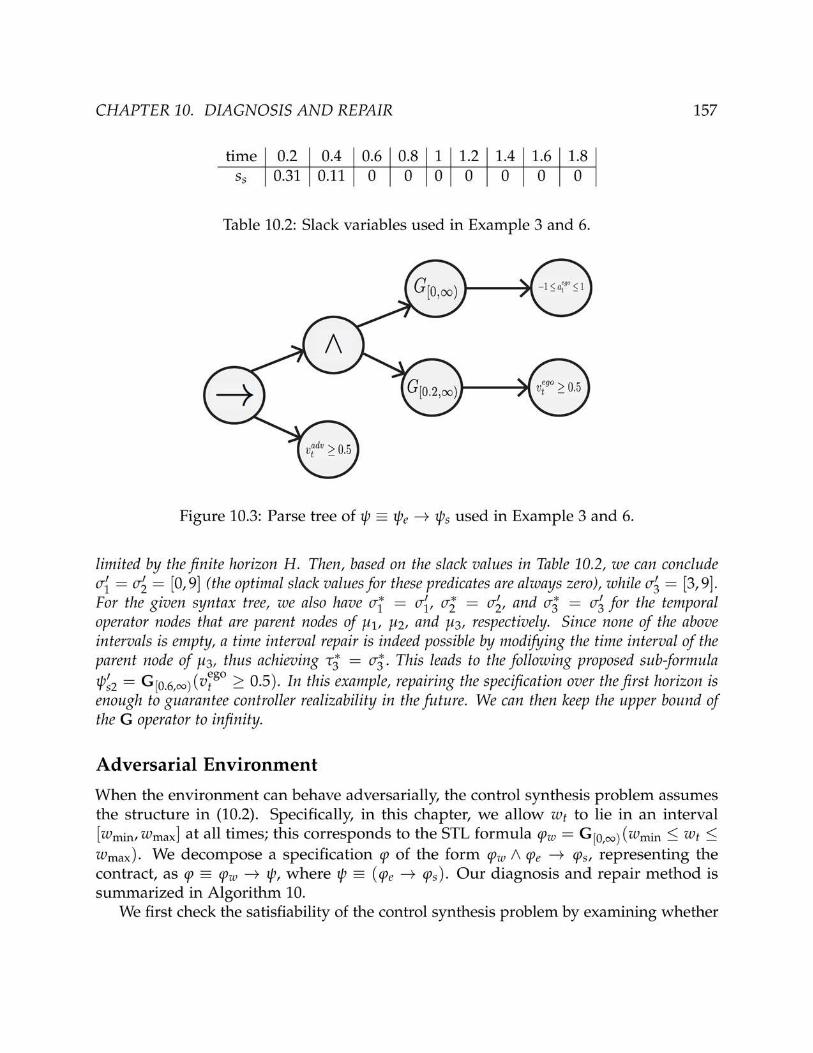

CHAPTER 10. DIAGNOSIS AND REPAIR 158
Algorithm 10 Diagnose Repair Adversarial
1: Input: P2: Output: uH, P ′3: (J, C)← GenMILP(P)4: (uH
0 , wH0 , sat)← CheckSAT(J, C)
5: if sat then6: W∗cand ← SolveCEGIS(uH
0 ,P)7: Wcand ←W∗cand8: whileWcand 6= ∅ do9: Pw ← RepairAdversarial(Wcand,P)
10: Wcand ← SolveCEGIS(uH0 ,Pw)
11: end while12: Wcand ←W∗cand, Pψ ← P13: whileWcand 6= ∅ do14: Pψ ← DiagnoseRepair(Pψ)
15: Wcand ← SolveCEGIS(uH0 ,Pψ)
16: end while17: P ′ ← FindMin(Pw,Pψ)
18: end if
there exists a pair of uH and wH for which problem (10.2) is feasible (CheckSAT routine):
minimizeuH ,wH
J(ξ(x0, uH, wH))
subject to ξ(x0, uH, wH) |= ϕ
wH |= ϕw ∧ ϕe.
(10.16)
If problem (10.16) is unsatisfiable, we can use the techniques introduced in Section 10.4and 10.5 to diagnose and repair the infeasibility. Therefore, in the following, we assumethat (10.16) is satisfiable, hence there exist uH
0 and wH0 that solve (10.16).
To check realizability, we use the following CEGIS loop (SolveCEGIS routine) [148].By first fixing the control trajectory to uH
0 , we find the worst case disturbance trajectorywH
1 that minimizes the robustness value of ϕ by solving the following problem:
minimizewH
ρϕ(ξ(x0, uH, wH), 0)
subject to wH |= ϕe ∧ ϕw
(10.17)
with uH = uH0 . The optimal wH
1 from (10.17) will falsify the specification if the resulting
robustness value is below zero4. If this is the case, we look for a uH1 which solves (10.15)
4A tolerance ρmin can be selected to accommodate approximation errors, i.e., ρϕ(ξ(x0, uH0 , wH
1 ), 0) <ρmin.

CHAPTER 10. DIAGNOSIS AND REPAIR 159
with the additional restriction of wH ∈ Wcand = wH1 . If this step is feasible, we once
again attempt to find a worst-case disturbance sequence wH2 that solves (10.17) with
uH = uH1 : this is the counterexample-guided inductive step. At each iteration i of this
CEGIS loop, the set of candidate disturbance sequences Wcand expands to include wHi .
If the loop terminates at iteration i with a successful uHi (one for which the worst case
disturbance wHi in (10.17) has positive robustness), we conclude that the formula ϕ is
realizable.The CEGIS loop may not terminate if the set Wcand is infinite. We, therefore, run it
for a maximum number of iterations. If SolveCEGIS fails to find a controller sequenceprior to the timeout, then (10.15) is infeasible for the current Wcand, i.e., there is nocontrol input that can satisfy ϕ for all disturbances in Wcand. We conclude that thespecification is not realizable (or, equivalently, the contract is inconsistent). While thisinfeasibility can be repaired by modifying ψ based on the techniques in Section 10.4and Section 10.5, an alternative solution is to repair ϕw by minimally pruning the boundson wt (RepairAdversarial routine).
To do so, given a small tolerance ǫ ∈ R+, we find
wu = maxwH
i ∈Wcand
t∈0,...,H−1
wi,t wl = minwH
i ∈Wcand
t∈0,...,H−1
wi,t (10.18)
and define su = wmax−wu and sl = wl −wmin. We then use su and sl to update the rangefor wt in ϕw to a maximal interval [w′min, w′max] ⊆ [wmin, wmax] and such that at least onewH
i ∈ Wcand is excluded. Specifically, if su ≤ sl, we set [w′min, w′max] = [wmin, wu − ǫ];otherwise we set [w′min, w′max] = [wl + ǫ, wmax]. The smaller the value of ǫ, the larger theresulting interval.
Finally, we use the updated formula ϕ′w to run SolveCEGIS again until a realizablecontrol sequence uH is found. For improved efficiency, the linear search proposed aboveto find the updated bounds w′min and w′max can be replaced by a binary search. Moreover,in Algorithm 10, assuming a predicate repair procedure, FindMin provides the solutionwith minimum slack norm between the ones repairing ψ and ϕw.
Example 7 (Adversarial Race). We consider the specification in Example 4. For the samehorizon as in the previous examples, after solving the satisfiability problem, for the fixed uH
0 , the
CEGIS loop returns aadvt = 2 for all t ∈ 0, . . . , H− 1 as the single element inWcand for which
no controller sequence can be found. We then choose to tighten the environment assumptionsto make the controller realizable, by shrinking the bounds on aadv
t by using Algorithm 10 withǫ = 0.01. After a few iterations, we finally obtain w′min = 0 and w′max = 1.24, and therefore
φ′w = G[0,∞)
(
0 ≤ aadvt ≤ 1.24
)
.
To account for the error introduced by ǫ, given ϕ′ ∈ REPAIRD,T (ϕ), we say that (ϕ′,D, T ) are ǫ-minimal if the magnitudes of the predicate repairs (predicate slacks) ortime-interval repairs differ by at most ǫ from a minimal repair in the sense of Problem

CHAPTER 10. DIAGNOSIS AND REPAIR 160
11. Assuming that SolveCEGIS terminates before reaching the maximum number ofiterations5, the following theorems state the properties of Algorithm 10.
Theorem 14 (Soundness). Given a controller synthesis problem P = ( fd, x0, ϕ, J), suchthat (10.2) is infeasible at time t, let ϕ′ ∈ REPAIRD,T (ϕ) be the repaired formula returnedfrom Algorithm 10 for a given set of predicates D or time interval T . Then, P ′ = ( fd, x0, ϕ′, J)is feasible at time t and (ϕ′, D, T ) is ǫ-minimal.
Proof (Theorem 14). We recall that ϕ ≡ ϕw → ψ. Moreover, Algorithm 10 provides thesolution with minimum slack norm between the ones repairing ψ and φw in the case ofpredicate repair. Then, when ψ = ϕe → ϕs is modified using Algorithm 7, soundness isguaranteed by Theorem 12 and the termination of the CEGIS loop. On the other hand,assume Algorithm 10 modifies the atomic predicates in φw. Then, the RepairArdversarialroutine and (10.18), together with the termination of the CEGIS loop, assure that ϕw isalso repaired in such a way that the controller is realizable, and ǫ-optimal (i.e., the lengthof the bounding box around wt differs from the maximal interval length by at most ǫ),which concludes our proof.
Theorem 15 (Completeness). Assume the controller synthesis problem P = ( fd, x0, ϕ, J) re-sults in (10.2) being infeasible at time t. If there exist a set of predicates D and time-intervals Tsuch that there exists Φ ⊆ REPAIRD,T (ϕ) for which ∀ φ ∈ Φ, P ′ = ( fd, x0, φ, J) is feasible attime t and (φ, D, T ) is ǫ-minimal, then Algorithm 10 returns a repaired formula ϕ′ in Φ.
Proof (Theorem 15). As discussed in the proof of Theorem 14, if Algorithm 10 modifiesψ = ϕe → ϕs using Algorithm 7, completeness is guaranteed by Theorem 13 andthe termination of the CEGIS loop. On the other hand, let us assume there exists aminimum norm repair for the atomic predicates of ϕw, which returns a maximal interval[w′min, w′max] ⊆ [wmin, wmax]. Then, given the termination of the CEGIS loop, by repeatedlyapplying (10.18) and RepairAdversarial, we produce a predicate repair such that thecorresponding interval [w′′min, w′′max] makes the control synthesis realizable and is maximalwithin an error bounded by ǫ (i.e., its length differs by at most ǫ from the one of themaximal interval [w′min, w′max]). Hence, ϕ′ ∈ Φ holds.
10.6 Case Studies
We developed the toolbox DiaRY (Diagnosis and Repair for sYnthesis)6 implementingour algorithms. DiaRY uses Yalmip [114] to formulate the optimization problems and
5Under failing assumptions, Algorithm 10 terminates with UNKNOWN.6https://github.com/shromonag/DiaRY

CHAPTER 10. DIAGNOSIS AND REPAIR 161
Gurobi [73] to solve them. It interfaces to different synthesis tools, e.g., BluSTL7 andCrSPrSTL8. Here, we summarize some of the results of DiaRY for diagnosis and repair.
Autonomous Driving
We consider the problem of synthesizing a controller for an autonomous vehicle in acity driving scenario. We analyze the following two tasks: (i) changing lanes on a busyroad; (ii) performing an unprotected left turn at a signalized intersection. We use thedynamics model introduced in Chapter 2.4. To determine the control strategy, we linearizethe overall system dynamics around the initial state at each run of the MPC, which iscompleted in less than 2 s on a 2.3-GHz Intel Core i7 processor with 16-GB memory. Wefurther impose the following constraints on the ego vehicle (i.e., the vehicle under control):(i) a minimum distance must be established between the ego vehicle and other cars on theroad to avoid collisions; (ii) the ego vehicle must obey the traffic lights; (iii) the ego vehiclemust stay within its road boundaries.
Lane Change
We consider a lane change scenario on a busy road as shown in Figure 10.4a. The egovehicle is in red. Car 1 is at the back of the left lane, Car 2 is in the front of the leftlane, while Car 3 is on the right lane. The states of the vehicles are initialized as follows:xCar 1
0 = [−0.2 − 1.5 π2 0.5]⊤, xCar 2
0 = [−0.2 1.5 π2 0.5]⊤, xCar 3
0 = [0.2 1.5 π2 0]⊤, and
xego0 = [0.2 − 0.7 π
2 0]⊤. The control inputs for ego and Car 3 are initialized at [0 0]⊤;
the ones for Car 1 and Car 2 are set to uCar 10 = [0 1]⊤ and uCar 2
0 = [0 − 0.25]⊤. Theobjective of ego is to safely change lane, while satisfying the following requirements:
ϕstr = G[0,∞)(|u1| ≤ 2) Steering Bounds
ϕacc = G[0,∞)(|u2| ≤ 1) Acceleration Bounds
ϕvel = G[0,∞)(|v| ≤ 1) Velocity Bounds
(10.19)
The solid blue line in Figure 10.4 is the trajectory of ego as obtained from our MPC scheme,while the dotted green line is the future trajectory pre-computed for a given horizon at agiven time. MPC becomes infeasible at time t = 1.2 s when the no-collision requirementis violated, and a possible collision is detected between the ego vehicle and Car 1 beforethe lane change is completed (Fig. 10.4a). Our solver takes 2 s, out of which 1.4 s areneeded to generate all the IISs, consisting of 39 constraints. To make the system feasible,the proposed repair increases both the acceleration bounds and the velocity bounds on
7https://github.com/BluSTL/BluSTL8https://github.com/dsadigh/CrSPrSTL

CHAPTER 10. DIAGNOSIS AND REPAIR 162
(a) (b)
Figure 10.4: Changing lane is infeasible at t = 1.2 s in (a) and is repaired in (b).
the ego vehicle as follows:
ϕnewacc = G[0,∞)(|u2| ≤ 3.5)
ϕnewvel = G[0,∞)(|v| ≤ 1.54).
(10.20)
When replacing the initial requirements ϕacc and ϕvel with the modified ones, the revisedMPC scheme allows the vehicle to travel faster and safely complete a lane changemaneuver, without risks of collision, as shown in Figure 10.4b.
Unprotected Left Turn
In the second scenario, we would like the ego vehicle to perform an unprotected leftturn at a signalized intersection, where the ego vehicle has a green light and is supposedto yield to oncoming traffic, represented by the yellow cars crossing the intersectionin Figure 10.5. The environment vehicles are initialized at the states xCar 1
0 = [−0.2 0.7 −π2 0.5]⊤ and xCar 2
0 = [−0.2 1.5 − π2 0.5]⊤, while the ego vehicle is initialized at x
ego0 =
[0.2 − 0.7 π2 0]⊤. The control input for each vehicle is initialized at [0 0]⊤. Moreover,
we use the same bounds as in (10.19).The MPC scheme becomes infeasible at t = 2.1 s. The solver takes 5 s, out of which
2.2 s are used to generate the IISs, including 56 constraints. As shown in Figure 10.5a, theego vehicle yields in the middle of intersection for the oncoming traffic to pass. However,the traffic signal turns red in the meanwhile, and there is no feasible control input for theego vehicle without breaking the traffic light rules. Since we do not allow modifications tothe traffic light rules, the original specification is repaired again by increasing the bounds

CHAPTER 10. DIAGNOSIS AND REPAIR 163
(a) (b)
Figure 10.5: Left turn becomes infeasible at time t = 2.1 s in (a) and is repaired in (b).
on acceleration and velocity, thus obtaining:
ϕnewacc = G[0,∞)
(
|u2| ≤ 11.903)
ϕnewvel = G[0,∞)
(
|v| ≤ 2.42)
.(10.21)
As shown by the trajectory in Figure 10.5b, under the assumptions and initial condi-tions of our scenario, higher allowed velocity and acceleration make the ego vehicle turnbefore the oncoming cars get close or cross the intersection.
Quadrotor Control
We assume a quadrotor dynamical model similar to the one discussed in Chapter 2.4.Our goal is to synthesize a strategy for the quadrotor to travel from a starting position
[x0, y0, z0] = [0, 0,−0.4] with zero roll, pitch, and yaw angles, i.e., [φ0, θ0, ψ0] = [0, 0, 0], toa destination [xd, yd, zd] = [1, 1,−0.1], still with zero roll, pitch, and yaw. All the otherelements in the state vector and the control input are initialized at zero. We define thefollowing constraints on the quadrotor:
ϕh = G[0,∞)(−1.1 ≤ z ≤ 0) Height of Flight Bounds
ϕroll = G[0,∞)(|u1| ≤ 0.3) Roll Bounds
ϕpitch = G[0,∞)(|u2| ≤ 0.3) Pitch Bounds
ϕthr = G[0,∞)(0 ≤ u4 ≤ 6.5) Thrust Bounds.
(10.22)
Our MPC scheme becomes infeasible at time t = 0.675 s because ϕh and ϕroll are bothviolated. Given the bounds on the control inputs, the trajectory is not guaranteed to lie in


CHAPTER 10. DIAGNOSIS AND REPAIR 165
the desired region. This is visualized in Figure 10.6 (a) and (c), respectively showing atwo-dimensional and three-dimensional projection of the quadrotor trajectory. The solidblue line shows the path computed by the MPC framework and taken by the quadrotor,aiming at traveling from the origin, marked by a black square, to the target, marked bya red square. Because of the bounds on the control inputs, the quadrotor touches theboundary of the allowed region (along the z axis) at t = 0.675 s.
The solver takes less than 0.1 s to generate the IIS, including 32 constraints, out ofwhich 11 constraints are associated with the predicates in ϕh and ϕroll. Our algorithmadds a slack of 1.58 to the upper bound on z in ϕh. We then modify ϕh to:
ϕnewh = G[0,∞)(−1.1 ≤ z ≤ 1.58), (10.23)
thus allowing the quadrotor to violate the upper bound on the vertical position duringthe maneuver. The new specification makes the problem realizable, and the resultingtrajectory is shown in blue in Figure 10.6 (b) and (d). We can view the above slackas the estimated margin from the boundary needed for the quadrotor to complete themaneuver based on the linearized model of the dynamics. As apparent from Figure 10.6b,such a margin is much larger than the space actually used by the quadrotor to completeits maneuver. A better estimate can be achieved by using a finer time interval forlinearizing the dynamics and executing the controller. While the solution above providesthe minimum slack norm for the given linearization, it is still possible to notify DiaRYthat ϕh must be regarded as a hard constraint, e.g., used to mark a rigid obstacle. In thiscase, DiaRY tries to relax the bounds on the control inputs to achieve feasibility.
10.7 Chapter Summary
We presented a set of algorithms for diagnosis and repair of STL specifications in thesetting of controller synthesis for hybrid systems using a model predictive control scheme.Given an unrealizable specification, our algorithms can detect possible reasons for in-feasibility and suggest repairs to make it realizable. We showed the effectiveness of ourapproach on the synthesis of controllers for several applications. As future work, weplan to investigate techniques that better leverage the structure of the STL formulae andextend to a broader range of environment assumptions in the adversarial setting.

166
Chapter 11
Final Words
We envision a world where autonomous systems are interacting with us seamlessly.Robots are integrated into our society, and are cognizant of their interaction with eachother, with the humans, and the environment they live in. They are also capable ofreasoning about their actions, and they plan safe strategies that humans can trust andrely on.
This thesis has been a key step towards the goal of understanding and designinga framework for modeling the interaction between humans and other agents, which iscrucial for correct-by-construction design and analysis of human-robot systems. In thischapter, we would like to conclude this dissertation by reflecting on our approach anddiscussing some of the limitations and future directions.
We have focused on two main control approaches in this work: interaction-aware control,and safe control.
Our work in interaction-aware control requires models of humans and the interactionbetween the human and autonomy as we have discussed in Chapter 3, Chapter 4,and Chapter 5. In Chapter 6, we have addressed the initial steps in increasing trust inhuman models by studying individual variations from learned human models. However,there are still many avenues to explore in designing better and more accurate modelsof humans in safety-critical human-robot systems such as approaches in behavioraleconomics to model human’s bounded rationality [66]. Similarly, we have used activemethods in learning human’s reward functions for both information gathering andcomparison-based learning (Chapter 4, Chapter 5). Such active learning techniquesenable us to only extract informative data and quickly converge to the desired outcome.In the future, we plan to utilize such methods in automatic testing and validation ofhuman-robot systems.
Our work in safe control, addresses correct-by-construction control from temporallogic specifications in reactive, continuous, and probabilistic settings (Chapter 7,Chap-ter 8, and Chapter 9). However, as more learning components are used in control andestimation of robotics systems, our formal techniques need to be modified to addresssafety guarantees in such settings. Chapter 9 is only a first step towards this direction, and

CHAPTER 11. CHAPTER:FINAL WORDS 167
future work in control and verification needs to address the challenges in safe and verifiedAI. We discuss some of these challenges in the next section. Further, in Chapter 10, westudied the problem of diagnosing and repairing infeasible specifications. Similarly, asmore data-driven and learned components appear in our systems, we are required todesign algorithms that are capable of diagnosis and repair with such learned components,which is in the direction of addressing various challenges in explainable and accountableAI.
11.1 Challenges in Safe and Interactive AI
Systems that heavily use AI, henceforth referred to as AI-based systems, have had asignificant impact in society in domains that include healthcare, transportation, socialnetworking, e-commerce, education, etc. This growing societal-scale impact has broughtwith it a set of risks and concerns including errors in AI software, cyber-attacks, andsafety of AI-based systems [153, 42, 10]. As we have seen in this dissertation, the AI-basedsystems have had an incredible impact on the design and control of human-robot systems.We address some of the challenges that need to be addressed in safe and interactive AIfor human-robot systems. Some of the material in this section appeared in [164], and werefer the reader to that paper for further details.
Environment Modeling
In the traditional success stories for formal verification, such as verifying cache coherenceprotocols or device drivers, the interface between the system and its environment iswell defined. Moreover, while the environment itself may not be known, it is usuallyacceptable to model it as a non-deterministic process subject to constraints specified in asuitable logic or automata-based formalism. Typically such an environment model is“over-approximate”, meaning that it may include more environment behaviors than arepossible.
We see systems based on AI or machine learning (ML) as being quite different.Consider an autonomous vehicle operating in rush-hour traffic in an urban environment.It may be impossible even to precisely define the interface between the system andenvironment (i.e., to identify the variables/features of the environment that must bemodeled), let alone to model all possible behaviors of the environment. Even if theinterface is known, non-deterministic or over-approximate modeling is likely to producetoo many spurious bug reports, rendering the verification process useless in practice.
Similarly, for human-robot systems, human agents are a key part of the environmentand/or system. Researchers have attempted modeling humans as non-deterministic orstochastic processes with the goal of verifying the correctness of the overall system [152,157]. Given the variability and uncertainty in human behavior, a data-driven approachbased on machine learning is usually necessary. Such an approach, in turn, is sensitive to

CHAPTER 11. CHAPTER:FINAL WORDS 168
the quality of data. For example, the technique of inverse reinforcement learning [128]can be used for learning the reward function of human agents [2, 188]. However, accuracyof the learned reward function depends on the expressivity of the hand-coded features bythe designer and the amount and variety of the data collected. In order to achieve verifiedAI for such human-in-the-loop systems, we need to address the limitations of the currenthuman modeling techniques and provide guarantees about their prediction accuracy andconvergence. When learned models are used, one must represent any uncertainty inthe learned parameters as a first-class entity in the model, and take that into account inverification and control. The challenge, then, is to come up with a method of environmentmodeling that allows one to provide provable guarantees on the system’s behavior evenwhen there is considerable uncertainty about the environment.
Formal Specification
Formal verification critically relies on having a formal specification – a precise, mathemat-ical statement of what the system is supposed to do. However, the challenge of comingup with a high-quality formal specification is well known, even in application domains inwhich formal verification has found considerable success (see, e.g., [22]).
This challenge is only exacerbated in AI-based systems. Consider a module in anautonomous vehicles that performs object recognition, distinguishing humans from otherobjects. What is the specification for such a module? How might it differ from thespecifications used in traditional applications of formal methods? What should thespecification language be, and what tools can one use to construct a specification?
Thus, we need to find an effective method to specify desired and undesired propertiesof systems that use AI- or ML-based components.
Modeling Systems that Learn
In most traditional applications of formal verification, the system is precisely known: itis a C program, or a circuit described in a hardware description language. The systemmodeling problem is primarily concerned with reducing the size of the system to a moretractable representation by abstracting away irrelevant details.
AI-based systems lead to a very different challenge for system modeling. A majorchallenge is the use of machine learning, where the system evolves as it encounters newdata and new situations. Modeling a deep neural network that has been trained onmillions of data points can be challenging enough even if one “freezes” the trainingprocess: new abstraction techniques will be necessary. Additionally, the verificationprocedure must account for future changes in the learner as new data arrives. Newtechniques must be devised to formally model components based on machine learning.
CHAPTER 11. CHAPTER:FINAL WORDS 169
Generating Training Data
Formal methods has proved effective for the systematic generation of test data in varioussettings including simulation-based verification of circuits (e.g., [93]) and finding securityexploits in commodity software (e.g., [15]). In these cases, even though the end result isnot a proof of correctness of the system, the generated tests raise the level of assurance inthe system’s correctness. Can the testing of AI-based systems leverage formal methods ina similar manner?
We have seen that various machine learning algorithms can fail under small adversarialperturbations [130, 57, 123, 70]. Learning algorithms promise to generalize from data,but such simple perturbations that fool the algorithms create concerns regarding theiruse in safety-critical applications such as autonomous driving. Such small perturbationsmight be even unrecognizable to humans, but drive the algorithm to misclassify theperturbed data. Recent efforts have started to combine ideas from formal methods andmachine learning to address problems such as compositional falsification of machinelearning components [48]. There are still many challenges left to devise techniques basedon formal methods to systematically generate training and testing data for ML-basedcomponents.
Active Test Scenario Generation
Efficiently and actively generating test scenarios is also a key factor in verification ofhuman-robot systems. For example, in the context of autonomous driving, today’sautomated cars measure the reliability of autonomy by the number of miles driven.However, the quality of driven miles is more important than its quantity. Using thepower of formal methods through model checking and counterexample-based techniques,one challenge is to automatically generate representative test scenarios for human-robotsystems in order to detect the interesting corner cases that potentially result in accidents.
Scalability of Verification and Optimization Engines
A constant question asked of formal verification is whether it can scale up to handleindustrial designs. Much progress has been made in this regard, especially in the area ofhardware verification, where formal methods are a standard part of the design flow.
However, in systems that use AI or ML, the scalability challenge is even greater.In addition to the scale of systems as measured by traditional metrics (dimension ofstate space, number of components, etc.), the types of components can be much morecomplex. For instance, in (semi-)autonomous driving, autonomous vehicles and theircontrollers need to be modeled as hybrid systems combining both discrete and continuousdynamics. Moreover, agents in the environment (humans, other vehicles) may needto be modeled as probabilistic processes. Finally, the requirements may involve not only

CHAPTER 11. CHAPTER:FINAL WORDS 170
traditional Boolean specifications on safety and liveness, but also quantitative requirementson system robustness and performance.
On a similar note, many of the performance measures or reward functions discussedin this dissertation are nonlinear and non-convex. Another challenge is to design scalablenonlinear optimization techniques that enable real-time computation for synthesizingsafe and interaction-aware controllers.
Human’s Bounded Rationality
Designing a framework for interaction between humans and autonomy requires illus-trative learned human models. Under the assumption that humans are approximatelyrational, we have used the principle of maximum entropy to learn their reward func-tions [159, 158, 160]. However, in many extreme events (e.g., car accidents), human actionscannot be explained as agents who optimize a rational reward function. Understandingand modeling such extreme cases is an essential component in providing guaranteesabout human-robot systems. We believe exploring ideas from behavioral economicscan facilitate designing systems that are aware of humans’ bounded rationality [66].This potentially further enables inference of probability of loss in such events and pro-vides a systematic design of insurance mechanisms for semiautonomous systems (e.g.,autonomous vehicles driving on roads shared with humans).
Human Variations
Data-driven human models such as human reward functions are usually constructedbased on large datasets that give access to a single model of rationality. However, humansvary in how they handle different situations, and we cannot fit a single model to allhumans. In safety-critical scenarios, we need to be able to quantize and measure howhumans can differ from the fitted model. As a step towards verified human modeling, wehave constructed an efficient (almost linear) algorithm to quantize and learn a distributionover the variations from the fitted model by querying individual humans on activelygenerated scenarios (see Chapter 6). However, more work is required in robustnessanalysis of human models in order to be able to use these results in control. Our workin Chapter 6 finds a sequence of falsifying actions for humans; however, one challenge isto utilize this falsifying sequence in an online manner to close the loop by synthesizingresilient controllers to human variations.
Shared Transportation Networks for Human-Robot Systems
Going beyond single agent systems, another challenging problem is to address human-robot systems at the system level, and explore its fundamental limits. Imagine a trans-portation network with fleets of autonomous and human-driven vehicles. If there are

CHAPTER 11. CHAPTER:FINAL WORDS 171
no human-driven vehicles, a central authority can plan routes for vehicles so as to min-imize the total cost. Moreover, if there are no autonomous vehicles, vehicles follow anequilibrium, which might have a suboptimal total cost. The cost of an equilibrium canbe worse than the optimum by a factor known as the price of anarchy. As systems movetowards semiautonomy, it is important to study scenarios that fall in between the twoextremes. Scenarios in which some vehicles (autonomous) can be routed by a centralauthority and the rest follow an equilibrium (that depends on the choices of the centralauthority). The study of these scenarios requires combining optimization techniques (forthe central authority) with game theoretic ideas (for human-driven vehicles).
11.2 Closing Thoughts
Our work presented in this dissertation is only a step that attempts to bring ideas fromrobotics, control theory, and formal methods to address the problems in the design,control, learning, and verification of human-robot systems. As discussed in this chapter,there are still many existing challenges that need to be addressed for safe and interactiveautonomy. We envision a strong collaboration between learning and control, human-robotinteraction, and formal methods communities to take advantage of both data-driven andmodel-based techniques in an effort to seamlessly integrate safe and reliable human-robotsystems in our society.

172
Bibliography
[1] H. Abbas et al. “Robustness-Guided Temporal Logic Testing and Verificationfor Stochastic Cyber-Physical Systems”. In: Proc. of IEEE International Conferenceon CYBER Technology in Automation, Control, and Intelligent Systems. 2014 (cit. onp. 108).
[2] P. Abbeel and A. Y. Ng. “Apprenticeship learning via inverse reinforcement learn-ing”. In: Proceedings of the twenty-first international conference on Machine learning.ACM. 2004, p. 1 (cit. on p. 168).
[3] P. Abbeel and A. Y. Ng. “Exploration and apprenticeship learning in reinforcementlearning”. In: Proceedings of the 22nd international conference on Machine learning.ACM. 2005, pp. 1–8 (cit. on pp. 3, 17, 29, 31).
[4] N. Ailon and M. Mohri. “Preference-based learning to rank”. In: Machine Learning80.2-3 (2010), pp. 189–211 (cit. on p. 62).
[5] A. K. Akametalu et al. “Reachability-based safe learning with gaussian processes”.In: 2014 IEEE 53rd Annual Conference on Decision and Control, pp. 1424–1431 (cit. onp. 124).
[6] B. Akgun et al. “Keyframe-based learning from demonstration”. In: InternationalJournal of Social Robotics 4.4 (2012), pp. 343–355 (cit. on p. 62).
[7] R. Akrour, M. Schoenauer, and M. Sebag. “April: Active preference learning-based reinforcement learning”. In: Joint European Conference on Machine Learningand Knowledge Discovery in Databases. Springer. 2012, pp. 116–131 (cit. on p. 62).
[8] R. Alur, S. Moarref, and U. Topcu. “Counter-strategy guided refinement of GR(1)temporal logic specifications”. In: Proceedings of the 13th Conference on Formal Meth-ods in Computer-Aided Design (FMCAD’13). 2013, pp. 26–33 (cit. on pp. 106, 108).
[9] R. Alur, S. Moarref, and U. Topcu. “Counter-strategy guided refinement of GR(1)temporal logic specifications”. In: Formal Methods in Computer-Aided Design. 2013(cit. on p. 141).
[10] D. Amodei et al. “Concrete Problems in AI Safety”. In: arXiv preprintarXiv:1606.06565 (2016) (cit. on p. 167).

BIBLIOGRAPHY 173
[11] G. Andrew and J. Gao. “Scalable training of L1-regularized log-linear models”.In: Proceedings of the 24th international conference on Machine learning. ACM. 2007,pp. 33–40 (cit. on pp. 31, 66).
[12] C. Andrieu et al. “An introduction to MCMC for machine learning”. In: Machinelearning 50.1-2 (2003), pp. 5–43 (cit. on p. 125).
[13] A. Aswani et al. “Provably safe and robust learning-based model predictivecontrol”. In: Automatica 49.5 (2013), pp. 1216–1226 (cit. on p. 124).
[14] R. J. Aumann, M. Maschler, and R. E. Stearns. Repeated games with incompleteinformation. MIT press, 1995 (cit. on p. 28).
[15] T. Avgerinos et al. “Automatic exploit generation”. In: Commun. ACM 57.2 (2014),pp. 74–84 (cit. on p. 169).
[16] M. Awais and D. Henrich. “Human-robot collaboration by intention recognition us-ing probabilistic state machines”. In: Robotics in Alpe-Adria-Danube Region (RAAD),2010 IEEE 19th International Workshop on. IEEE. 2010, pp. 75–80 (cit. on p. 43).
[17] C. L. Baker, R. Saxe, and J. B. Tenenbaum. “Action understanding as inverseplanning”. In: Cognition 113.3 (2009), pp. 329–349 (cit. on p. 43).
[18] T. Bandyopadhyay et al. “Intention-aware motion planning”. In: Algorithmic Foun-dations of Robotics X. Springer, 2013, pp. 475–491 (cit. on pp. 5, 43).
[19] F. Bastien et al. Theano: new features and speed improvements. Deep Learning andUnsupervised Feature Learning NIPS 2012 Workshop. 2012 (cit. on p. 32).
[20] C. Basu et al. “Do you want your autonomous car to drive like you?” In: 2017 12thACM/IEEE International Conference on Human-Robot Interaction (HRI). IEEE. 2017(cit. on p. 62).
[21] M. J. Beal. Variational algorithms for approximate Bayesian inference. University ofLondon, 2003 (cit. on pp. 125, 139).
[22] I. Beer et al. “Efficient Detection of Vacuity in ACTL Formulas”. In: Formal Methodsin System Design 18.2 (2001), pp. 141–162 (cit. on p. 168).
[23] A. Bemporad and M. Morari. “Control of systems integrating logic, dynamics,and constraints”. In: Automatica 35.3 (1999), pp. 407–427. doi: 10.1016/S0005-1098(98)00178-2. url: http://dx.doi.org/10.1016/S0005-1098(98)00178-2(cit. on pp. 108, 142).
[24] A. Bemporad and M. Morari. “Robust model predictive control: A survey”. In:Robustness in identification and control. Springer, 1999, pp. 207–226 (cit. on p. 141).
[25] A. Ben-Tal, L. El Ghaoui, and A. Nemirovski. Robust optimization. Princeton Uni-versity Press, 2009 (cit. on p. 129).
[26] J. Bergstra et al. “Theano: a CPU and GPU Math Expression Compiler”. In: Pro-ceedings of the Python for Scientific Computing Conference (SciPy). Oral Presentation.Austin, TX, June 2010 (cit. on p. 32).

BIBLIOGRAPHY 174
[27] D. S. Bernstein et al. “The complexity of decentralized control of Markov decisionprocesses”. In: Mathematics of operations research 27.4 (2002), pp. 819–840 (cit. onp. 28).
[28] A. Biere et al. “Symbolic Model Checking without BDDs”. In: Tools and Algo-rithms for Construction and Analysis of Systems, 5th International Conference, TACAS’99, Held as Part of the European Joint Conferences on the Theory and Practice of Soft-ware, ETAPS’99, Amsterdam, The Netherlands, March 22-28, 1999, Proceedings. 1999,pp. 193–207. doi: 10.1007/3-540-49059-0_14. url: http://dx.doi.org/10.1007/3-540-49059-0_14 (cit. on p. 108).
[29] L. Blackmore, M. Ono, and B. C. Williams. “Chance-constrained optimal pathplanning with obstacles”. In: 2011 IEEE Transactions on Robotics 27.6 (), pp. 1080–1094 (cit. on pp. 124, 129).
[30] R. Bloem et al. “RATSY - A New Requirements Analysis Tool with Synthesis.” In:CAV’10. 2010, pp. 425–429 (cit. on p. 104).
[31] S. Boyd and L. Vandenberghe. Convex optimization. Cambridge university press,2004 (cit. on pp. 129, 130).
[32] D. Braziunas. “Computational approaches to preference elicitation”. In: Departmentof Computer Science, University of Toronto, Tech. Rep (2006) (cit. on p. 62).
[33] K. Brinker, J. Fürnkranz, and E. Hüllermeier. Label ranking by learning pairwisepreferences. Tech. rep. Technical Report TUD-KE-2007-01, Knowledge EngineeringGroup, TU Darmstadt, 2007 (cit. on p. 62).
[34] J. R. Büchi. “Symposium on decision problems: On a decision method in restrictedsecond order arithmetic”. In: Studies in Logic and the Foundations of Mathematics 44(1966), pp. 1–11 (cit. on p. 19).
[35] E. F. Camacho and C. B. Alba. Model predictive control. Springer Science & BusinessMedia, 2013 (cit. on pp. 16, 29).
[36] A. Carvalho et al. “Stochastic Predictive Control of Autonomous Vehicles inUncertain Environments”. In: 12th International Symposium on Advanced VehicleControl. 2014 (cit. on p. 124).
[37] K. Chatterjee, T. A. Henzinger, and B. Jobstmann. “Environment Assumptionsfor Synthesis”. In: Proceedings of the 19th international conference on ConcurrencyTheory. CONCUR ’08. Toronto, Canada: Springer-Verlag, 2008, pp. 147–161. doi:http://dx.doi.org/10.1007/978-3-540-85361-9_14. url: http://dx.doi.org/10.1007/978-3-540-85361-9_14 (cit. on p. 106).
[38] K. Chatterjee et al. “Counterexample-guided Planning”. In: UAI ’05, Proceed-ings of the 21st Conference in Uncertainty in Artificial Intelligence, Edinburgh, Scot-land, July 26-29, 2005. 2005, pp. 104–111. url: http : / / uai . sis . pitt . edu /
displayArticleDetails.jsp?mmnu=1&smnu=2&article_id=1214&proceeding_
id=21 (cit. on p. 108).

BIBLIOGRAPHY 175
[39] J. W. Chinneck and E. W. Dravnieks. “Locating minimal infeasible constraint setsin linear programs”. In: ORSA Journal on Computing 3.2 (1991), pp. 157–168 (cit. onp. 149).
[40] M.-C. Costa, L. Léocart, and F. Roupin. “Minimal multicut and maximal integermultiflow: A survey”. In: European Journal of Operational Research 162.1 (2005),pp. 55–69 (cit. on p. 103).
[41] C. Daniel et al. “Active Reward Learning.” In: Robotics: Science and Systems. 2014(cit. on p. 64).
[42] T. G. Dietterich and E. J. Horvitz. “Rise of concerns about AI: reflections anddirections”. In: Communications of the ACM 58.10 (2015), pp. 38–40 (cit. on p. 167).
[43] X. C. Ding, M. Lazar, and C. Belta. “LTL receding horizon control for finitedeterministic systems”. In: Automatica 50.2 (2014), pp. 399–408. doi: 10.1016/j.automatica.2013.11.030. url: http://dx.doi.org/10.1016/j.automatica.2013.11.030 (cit. on p. 109).
[44] M. Dissanayake et al. “A solution to the simultaneous localization and mapbuilding (SLAM) problem”. In: Robotics and Automation, IEEE Transactions on 17.3(2001), pp. 229–241 (cit. on p. 8).
[45] A. Donzé and O. Maler. “Robust Satisfaction of Temporal Logic over Real-ValuedSignals”. In: Formal Modeling and Analysis of Timed Systems - 8th International Con-ference, FORMATS 2010, Klosterneuburg, Austria, September 8-10, 2010. Proceedings.2010, pp. 92–106. doi: 10.1007/978-3-642-15297-9_9. url: http://dx.doi.org/10.1007/978-3-642-15297-9_9 (cit. on p. 21).
[46] A. D. Dragan. “Robot Planning with Mathematical Models of Human State andAction”. In: arXiv preprint arXiv:1705.04226 (2017) (cit. on p. 28).
[47] A. D. Dragan and S. S. Srinivasa. Formalizing assistive teleoperation. MIT Press, July,2012 (cit. on p. 43).
[48] T. Dreossi, A. Donzé, and S. A. Seshia. “Compositional Falsification of Cyber-Physical Systems with Machine Learning Components”. In: NASA Formal MethodsSymposium. Springer. 2017, pp. 357–372 (cit. on p. 169).
[49] P. M. Esfahani, T. Sutter, and J. Lygeros. “Performance bounds for the scenario ap-proach and an extension to a class of non-convex programs”. In: IEEE Transactionson Automatic Control 60.1 (2015), pp. 46–58 (cit. on p. 113).
[50] F. A. A. (FAA). The Interfaces between Flight Crews and Modern Flight Systems. http://www.faa.gov/avr/afs/interfac.pdf. 1995 (cit. on p. 93).
BIBLIOGRAPHY 176
[51] G. E. Fainekos and G. J. Pappas. “Robust Sampling for MITL Specifications”. In:Formal Modeling and Analysis of Timed Systems, 5th International Conference, FOR-MATS 2007, Salzburg, Austria, October 3-5, 2007, Proceedings. 2007, pp. 147–162.doi: 10.1007/978-3-540-75454-1_12. url: http://dx.doi.org/10.1007/978-3-540-75454-1_12 (cit. on p. 23).
[52] G. E. Fainekos and G. J. Pappas. “Robustness of temporal logic specifications forcontinuous-time signals”. In: Theor. Comput. Sci. 410.42 (2009), pp. 4262–4291. doi:10.1016/j.tcs.2009.06.021. url: http://dx.doi.org/10.1016/j.tcs.2009.06.021 (cit. on p. 21).
[53] G. E. Fainekos et al. “Temporal logic motion planning for dynamic robots”. In:Automatica 45.2 (2009), pp. 343–352. doi: 10.1016/j.automatica.2008.08.008.url: http://dx.doi.org/10.1016/j.automatica.2008.08.008 (cit. on p. 107).
[54] P. Falcone et al. “Integrated braking and steering model predictive control approachin autonomous vehicles”. In: Advances in Automotive Control. Vol. 5. 1. 2007, pp. 273–278 (cit. on p. 8).
[55] P. Falcone et al. “MPC-based yaw and lateral stabilisation via active front steeringand braking”. en. In: Vehicle System Dynamics 46.sup1 (Sept. 2008), pp. 611–628(cit. on p. 8).
[56] P. Falcone et al. “Predictive Active Steering Control for Autonomous VehicleSystems”. In: IEEE Transactions on Control Systems Technology 15.3 (May 2007),pp. 566–580 (cit. on p. 8).
[57] A. Fawzi, O. Fawzi, and P. Frossard. “Analysis of classifiers’ robustness to adver-sarial perturbations”. In: arXiv preprint arXiv:1502.02590 (2015) (cit. on p. 169).
[58] A. Fern et al. “A Decision-Theoretic Model of Assistance.” In: IJCAI. 2007, pp. 1879–1884 (cit. on pp. 5, 43, 46).
[59] T. Ferrère, O. Maler, and D. Nickovic. “Trace Diagnostics Using Temporal Impli-cants”. In: Proc. Int. Symp. Automated Technology for Verification and Analysis. 2015(cit. on p. 141).
[60] J. Fu and U. Topcu. “Computational methods for stochastic control with metricinterval temporal logic specifications”. In: arXiv:1503.07193 (2015) (cit. on p. 124).
[61] J. Fu and U. Topcu. “Integrating active sensing into reactive synthesis with tempo-ral logic constraints under partial observations”. In: arXiv:1410.0083 (2014) (cit. onp. 124).
[62] D. Fudenberg and J. Tirole. “Game theory, 1991”. In: Cambridge, Massachusetts 393(1991) (cit. on p. 29).
[63] J. Fürnkranz et al. “Preference-based reinforcement learning: a formal frameworkand a policy iteration algorithm”. In: Machine learning 89.1-2 (2012), pp. 123–156(cit. on p. 62).

BIBLIOGRAPHY 177
[64] A. Gelman et al. Bayesian data analysis. Vol. 2. Taylor & Francis, 2014 (cit. on p. 125).
[65] S. Ghosh et al. “Diagnosis and repair for synthesis from signal temporal logicspecifications”. In: Proceedings of the 19th International Conference on Hybrid Systems:Computation and Control. ACM. 2016, pp. 31–40 (cit. on pp. 12, 124).
[66] G. Gigerenzer and R. Selten. Bounded rationality: The adaptive toolbox. MIT press,2002 (cit. on pp. 166, 170).
[67] J. H. Gillula and C. J. Tomlin. “Guaranteed safe online learning via reachability:tracking a ground target using a quadrotor”. In: 2012 IEEE International Conferenceon Robotics and Automation, pp. 2723–2730 (cit. on p. 124).
[68] E. A. Gol and M. Lazar. “Temporal logic model predictive control for discrete-time systems”. In: Proceedings of the 16th international conference on Hybrid systems:computation and control, HSCC 2013, April 8-11, 2013, Philadelphia, PA, USA. 2013,pp. 343–352. doi: 10.1145/2461328.2461379. url: http://doi.acm.org/10.1145/2461328.2461379 (cit. on p. 108).
[69] D. Golovin and A. Krause. “Adaptive submodularity: Theory and applicationsin active learning and stochastic optimization”. In: Journal of Artificial IntelligenceResearch 42 (2011), pp. 427–486 (cit. on p. 69).
[70] I. J. Goodfellow, J. Shlens, and C. Szegedy. “Explaining and harnessing adversarialexamples”. In: arXiv preprint arXiv:1412.6572 (2014) (cit. on p. 169).
[71] A. Gray et al. “Robust predictive control for semi-autonomous vehicles with anuncertain driver model”. In: Intelligent Vehicles Symposium (IV), 2013 IEEE. IEEE.2013, pp. 208–213 (cit. on p. 8).
[72] M. Green and D. J. Limebeer. Linear robust control. Courier Corporation, 2012(cit. on p. 124).
[73] Gurobi Optimizer. [Online]: http://www.gurobi.com/ (cit. on pp. 133, 149, 161).
[74] H. Haario, E. Saksman, and J. Tamminen. “An adaptive Metropolis algorithm”. In:Bernoulli (2001), pp. 223–242 (cit. on p. 67).
[75] E. A. Hansen, D. S. Bernstein, and S. Zilberstein. “Dynamic programming forpartially observable stochastic games”. In: AAAI. Vol. 4. 2004, pp. 709–715 (cit. onp. 28).
[76] T. Hedden and J. Zhang. “What do you think I think you think?: Strategic reasoningin matrix games”. In: Cognition 85.1 (2002), pp. 1–36 (cit. on pp. 3, 29).
[77] C. Hermes et al. “Long-term vehicle motion prediction”. In: 2009 IEEE IntelligentVehicles Symposium. 2009, pp. 652–657 (cit. on p. 8).
[78] R. Holladay et al. “Active Comparison Based Learning Incorporating User Uncer-tainty and Noise”. In: () (cit. on p. 62).

BIBLIOGRAPHY 178
[79] H. Huang et al. “Aerodynamics and control of autonomous quadrotor helicoptersin aggressive maneuvering”. In: 2009 IEEE International Conference on Robotics andAutomation. IEEE. 2009, pp. 3277–3282 (cit. on p. 24).
[80] A. Jain et al. “Learning preferences for manipulation tasks from online coactivefeedback”. In: The International Journal of Robotics Research (2015) (cit. on p. 62).
[81] S. Javdani, J. A. Bagnell, and S. Srinivasa. “Shared Autonomy via HindsightOptimization”. In: arXiv preprint arXiv:1503.07619 (2015) (cit. on pp. 5, 43, 46).
[82] S. Javdani et al. “Efficient touch based localization through submodularity”. In:Robotics and Automation (ICRA), 2013 IEEE International Conference on. IEEE. 2013,pp. 1828–1835 (cit. on p. 28).
[83] S. Jha and V. Raman. “Automated synthesis of safe autonomous vehicle controlunder perception uncertainty”. In: NASA Formal Methods Symposium. Springer.2016, pp. 117–132 (cit. on p. 124).
[84] X. Jin et al. “Mining requirements from closed-loop control models”. In: Proceed-ings of the 16th international conference on Hybrid systems: computation and control,HSCC 2013, April 8-11, 2013, Philadelphia, PA, USA. 2013, pp. 43–52. doi: 10.1145/2461328.2461337. url: http://doi.acm.org/10.1145/2461328.2461337 (cit. onp. 108).
[85] M. Jordan. “Learning in graphical models (adaptive computation and machinelearning)”. In: (1998) (cit. on pp. 123, 125).
[86] S. Karaman and E. Frazzoli. “Linear temporal logic vehicle routing with appli-cations to multi-UAV mission planning”. In: International Journal of Robust andNonlinear Control 21.12 (2011), pp. 1372–1395. doi: 10.1002/rnc.1715. url: http://dx.doi.org/10.1002/rnc.1715 (cit. on p. 107).
[87] S. Karaman and E. Frazzoli. “Linear temporal logic vehicle routing with appli-cations to multi-UAV mission planning”. In: International Journal of Robust andNonlinear Control 21.12 (2011), pp. 1372–1395 (cit. on p. 124).
[88] S. Karaman and E. Frazzoli. “Sampling-based motion planning with deterministic¯-calculus specifications”. In: Proceedings of the 48th IEEE Conference on Decisionand Control, CDC 2009, combined withe the 28th Chinese Control Conference, December16-18, 2009, Shanghai, China. 2009, pp. 2222–2229. doi: 10.1109/CDC.2009.5400278.url: http://dx.doi.org/10.1109/CDC.2009.5400278 (cit. on pp. 107, 124).
[89] S. Karaman and E. Frazzoli. “Vehicle Routing Problem with Metric Temporal LogicSpecifications”. In: Proceedings of the 47th IEEE Conference on Decision and Control,CDC 2008, December 9-11, 2008, Cancún, México. 2008, pp. 3953–3958. doi: 10.1109/CDC.2008.4739366. url: http://dx.doi.org/10.1109/CDC.2008.4739366 (cit. onpp. 107, 124).
[90] A. Karbasi, S. Ioannidis, et al. “Comparison-based learning with rank nets”. In:arXiv preprint arXiv:1206.4674 (2012) (cit. on p. 62).

BIBLIOGRAPHY 179
[91] S. Kataoka. “A stochastic programming model”. In: Econometrica: Journal of theEconometric Society (1963), pp. 181–196 (cit. on p. 130).
[92] E. C. Kerrigan and J. M. Maciejowski. “Soft constraints and exact penalty functionsin model predictive control”. In: Control Conference, Cambridge. 2000 (cit. on p. 141).
[93] N. Kitchen and A. Kuehlmann. “Stimulus generation for constrained random simu-lation”. In: Proceedings of the 2007 IEEE/ACM International Conference on Computer-Aided Design (ICCAD). IEEE Press. 2007, pp. 258–265 (cit. on p. 169).
[94] M. Kloetzer and C. Belta. “A Fully Automated Framework for Control of LinearSystems from Temporal Logic Specifications”. In: IEEE Trans. Automat. Contr. 53.1(2008), pp. 287–297. doi: 10.1109/TAC.2007.914952. url: http://dx.doi.org/10.1109/TAC.2007.914952 (cit. on p. 107).
[95] R. Könighofer, G. Hofferek, and R. Bloem. “Debugging formal specifications: apractical approach using model-based diagnosis and counterstrategies”. In: STTT15.5-6 (2013), pp. 563–583 (cit. on p. 141).
[96] M. V. Kothare, V. Balakrishnan, and M. Morari. “Robust constrained model predic-tive control using linear matrix inequalities”. In: Automatica 32.10 (1996), pp. 1361–1379 (cit. on p. 124).
[97] H. Kress-Gazit, G. Fainekos, and G. Pappas. “Temporal-Logic-Based ReactiveMission and Motion Planning”. In: IEEE Transactions on Robotics 25.6 (Dec. 2009),pp. 1370–1381. doi: 10.1109/TRO.2009.2030225 (cit. on pp. 95, 105, 124).
[98] M. Kuderer, S. Gulati, and W. Burgard. “Learning driving styles for autonomousvehicles from demonstration”. In: Proceedings of the IEEE International Conferenceon Robotics & Automation (ICRA), Seattle, USA. Vol. 134. 2015 (cit. on pp. 17, 31).
[99] D. Kulic and E. A. Croft. “Affective state estimation for human–robot interaction”.In: Robotics, IEEE Transactions on 23.5 (2007), pp. 991–1000 (cit. on p. 43).
[100] Y. Kwon and G. Agha. “LTLC: Linear Temporal Logic for Control”. In: HybridSystems: Computation and Control, 11th International Workshop, HSCC 2008, St. Louis,MO, USA, April 22-24, 2008. Proceedings. 2008, pp. 316–329. doi: 10.1007/978-3-540-78929-1_23. url: http://dx.doi.org/10.1007/978-3-540-78929-1_23(cit. on p. 107).
[101] L. T. Kohn and J. M. Corrigan and M. S. Donaldson, editors. To Err is Human:Building a Safer Health System. Tech. rep. National Academy Press. Washington,DC: A report of the Committee on Quality of Health Care in America, Institute ofMedicine, 2000 (cit. on p. 93).
[102] C.-P. Lam, A. Y. Yang, and S. S. Sastry. “An efficient algorithm for discrete-time hidden mode stochastic hybrid systems”. In: Control Conference (ECC), 2015European. IEEE. 2015, pp. 1212–1218 (cit. on pp. 43, 46).

BIBLIOGRAPHY 180
[103] K. Leahy et al. “Distributed information gathering policies under temporal logicconstraints”. In: 2015 IEEE 54th Annual Conference on Decision and Control (CDC),pp. 6803–6808 (cit. on p. 124).
[104] Y. T. Lee, A. Sidford, and S. C.-w. Wong. “A faster cutting plane method andits implications for combinatorial and convex optimization”. In: arXiv preprintarXiv:1508.04874 (2015) (cit. on p. 132).
[105] D. Lenz, T. Kessler, and A. Knoll. “Stochastic model predictive controller withchance constraints for comfortable and safe driving behavior of autonomousvehicles”. In: 2015 IEEE Intelligent Vehicles Symposium, pp. 292–297 (cit. on pp. 124,129).
[106] J. Leonard et al. “A perception-driven autonomous urban vehicle”. In: Journal ofField Robotics 25.10 (2008), pp. 727–774 (cit. on p. 8).
[107] S. Levine and V. Koltun. “Continuous inverse optimal control with locally optimalexamples”. In: arXiv preprint arXiv:1206.4617 (2012) (cit. on pp. 3, 17, 18, 29, 31, 48,64).
[108] J. Levinson et al. “Towards fully autonomous driving: Systems and algorithms”.In: 2011 IEEE Intelligent Vehicles Symposium (IV), pp. 163–168 (cit. on p. 8).
[109] W. Li, L. Dworkin, and S. A. Seshia. “Mining Assumptions for Synthesis”. In:Proceedings of the Ninth ACM/IEEE International Conference on Formal Methods andModels for Codesign (MEMOCODE). July 2011, pp. 43–50 (cit. on pp. 106, 141).
[110] W. Li et al. “Synthesis for Human-in-the-Loop Control Systems”. In: Proceedingsof the 20th International Conference on Tools and Algorithms for the Construction andAnalysis of Systems (TACAS). Apr. 2014, pp. 470–484 (cit. on pp. 6, 12, 94, 141).
[111] M. Liebner et al. “Driver intent inference at urban intersections using the intelli-gent driver model”. In: Intelligent Vehicles Symposium (IV), 2012 IEEE. IEEE. 2012,pp. 1162–1167 (cit. on p. 43).
[112] S. C. Livingston, R. M. Murray, and J. W. Burdick. “Backtracking temporal logicsynthesis for uncertain environments”. In: IEEE International Conference on Roboticsand Automation (ICRA). IEEE. 2012, pp. 5163–5170 (cit. on p. 105).
[113] S. C. Livingston et al. “Patching task-level robot controllers based on a localµ-calculus formula”. In: (2012) (cit. on p. 105).
[114] J. Löfberg. “YALMIP: A Toolbox for Modeling and Optimization in MATLAB”. In:Proceedings of the CACSD Conference. Taipei, Taiwan, 2004. url: http://users.isy.liu.se/johanl/yalmip (cit. on p. 160).
[115] J. Löfberg. “YALMIP: A toolbox for modeling and optimization in MATLAB”. In:2004 IEEE International Symposium on Computer Aided Control Systems Design. IEEE.2004, pp. 284–289 (cit. on p. 133).
BIBLIOGRAPHY 181
[116] M. Lopes, F. Melo, and L. Montesano. “Active learning for reward estimation ininverse reinforcement learning”. In: Joint European Conference on Machine Learningand Knowledge Discovery in Databases. Springer. 2009, pp. 31–46 (cit. on p. 64).
[117] L. Lovász and S. Vempala. “Fast algorithms for logconcave functions: Sampling,rounding, integration and optimization”. In: 2006 47th Annual IEEE Symposium onFoundations of Computer Science (FOCS’06). IEEE. 2006, pp. 57–68 (cit. on p. 67).
[118] B. Luders, M. Kothari, and J. P. How. “Chance constrained RRT for probabilisticrobustness to environmental uncertainty”. In: AIAA guidance, navigation, and controlconference (GNC), Toronto, Canada. 2010 (cit. on p. 8).
[119] O. Maler and D. Nickovic. “Monitoring Temporal Properties of Continuous Sig-nals”. In: Formal Techniques, Modelling and Analysis of Timed and Fault-Tolerant Sys-tems, Joint International Conferences on Formal Modelling and Analysis of Timed Sys-tems, FORMATS 2004 and Formal Techniques in Real-Time and Fault-Tolerant Systems,FTRTFT 2004, Grenoble, France, September 22-24, 2004, Proceedings. 2004, pp. 152–166. doi: 10.1007/978-3-540-30206-3_12. url: http://dx.doi.org/10.1007/978-3-540-30206-3_12 (cit. on p. 108).
[120] T. P. Minka. “A family of algorithms for approximate Bayesian inference”. PhDthesis. Massachusetts Institute of Technology, 2001 (cit. on pp. 125, 139).
[121] I. Mitchell, A. Bayen, and C. J. Tomlin. “A time-dependent Hamilton-Jacobi formu-lation of reachable sets for continuous dynamic games”. In: 2005 IEEE Transactionson Automatic Control 50.7 (), pp. 947–957 (cit. on p. 124).
[122] I. Mitchell and C. J. Tomlin. “Level set methods for computation in hybrid systems”.In: Hybrid Systems: Computation and Control. Springer, 2000, pp. 310–323 (cit. onp. 124).
[123] S.-M. Moosavi-Dezfooli, A. Fawzi, and P. Frossard. “DeepFool: a simple andaccurate method to fool deep neural networks”. In: arXiv preprint arXiv:1511.04599(2015) (cit. on p. 169).
[124] M. Morari et al. Model predictive control. Prentice Hall Englewood Cliffs, NJ, 1993(cit. on p. 15).
[125] R. Motwani and P. Raghavan. Randomized algorithms. Chapman & Hall/CRC, 2010(cit. on p. 115).
[126] R. M. Murray et al. “Online Control Customization via Optimization-Based Con-trol”. In: Software-Enabled Control. John Wiley & Sons, Inc., 2005, pp. 149–174. doi:10.1002/047172288X.ch9. url: http://dx.doi.org/10.1002/047172288X.ch9(cit. on p. 108).
[127] National Highway Traffic Safety Administration. Preliminary Statement of PolicyConcerning Automated Vehicles. May 2013 (cit. on p. 94).

BIBLIOGRAPHY 182
[128] A. Y. Ng and S. J. Russell. “Algorithms for Inverse Reinforcement Learning”. In:Proceedings of the Seventeenth International Conference on Machine Learning (ICML).2000, pp. 663–670 (cit. on p. 168).
[129] A. Y. Ng, S. J. Russell, et al. “Algorithms for inverse reinforcement learning.” In:Proceedings of the 17th international conference on Machine learning. 2000, pp. 663–670(cit. on pp. 3, 17, 29, 31).
[130] A. Nguyen, J. Yosinski, and J. Clune. “Deep neural networks are easily fooled:High confidence predictions for unrecognizable images”. In: 2015 IEEE Conferenceon Computer Vision and Pattern Recognition (CVPR). IEEE. 2015, pp. 427–436 (cit. onp. 169).
[131] T.-H. D. Nguyen et al. “Capir: Collaborative action planning with intention recog-nition”. In: arXiv preprint arXiv:1206.5928 (2012) (cit. on p. 43).
[132] S. Nikolaidis et al. “Formalizing Human-Robot Mutual Adaptation via a BoundedMemory Based Model”. In: Human-Robot Interaction. Mar. 2016 (cit. on p. 46).
[133] P. Nuzzo et al. “A Contract-Based Methodology for Aircraft Electric Power SystemDesign”. In: IEEE Access 2 (2014), pp. 1–25. doi: 10.1109/ACCESS.2013.2295764.url: http://dx.doi.org/10.1109/ACCESS.2013.2295764 (cit. on p. 107).
[134] P. Nuzzo et al. “CalCS: SMT Solving for Non-linear Convex Constraints”. In: IEEEInt. Conf. Formal Methods in Computer-Aided Design. 2010 (cit. on p. 141).
[135] P. Nuzzo et al. “A Contract-Based Methodology for Aircraft Electric Power SystemDesign”. In: IEEE Access 2 (2014), pp. 1–25. doi: 10.1109/ACCESS.2013.2295764(cit. on pp. 140, 142).
[136] P. Nuzzo et al. “A Platform-Based Design Methodology with Contracts and RelatedTools for the Design of Cyber-Physical Systems”. In: Proc. IEEE 103.11 (Nov. 2015)(cit. on pp. 140, 142).
[137] S. Patil et al. “Scaling up gaussian belief space planning through covariance-freetrajectory optimization and automatic differentiation”. In: Algorithmic Foundationsof Robotics XI. Springer, 2015, pp. 515–533 (cit. on p. 28).
[138] N. Piterman and A. Pnueli. “Synthesis of reactive(1) designs”. In: In Proc. Verifica-tion, Model Checking, and Abstract Interpretation (VMCAI’06. Springer, 2006, pp. 364–380 (cit. on p. 105).
[139] N. Piterman, A. Pnueli, and Y. Sa′ar. “Synthesis of reactive (1) designs”. In: Verifi-cation, Model Checking, and Abstract Interpretation, 2006. Springer. 2006, pp. 364–380(cit. on pp. 6, 124).
[140] E. Plaku and S. Karaman. “Motion planning with temporal-logic specifications:Progress and challenges”. In: AI Communications Preprint (), pp. 1–12 (cit. onp. 124).

BIBLIOGRAPHY 183
[141] A. Pnueli and R. Rosner. “On the synthesis of a reactive module”. In: Proceedings ofthe 16th ACM SIGPLAN-SIGACT symposium on Principles of programming languages.POPL ’89. Austin, Texas, United States: ACM, 1989, pp. 179–190. doi: http :
//doi.acm.org/10.1145/75277.75293. url: http://doi.acm.org/10.1145/75277.75293 (cit. on pp. 20, 105).
[142] A. Pnueli. “The Temporal Logic of Programs”. In: 18th Annual Symposium onFoundations of Computer Science (FOCS). 1977, pp. 46–57 (cit. on p. 19).
[143] S. Prentice and N. Roy. “The belief roadmap: Efficient planning in belief spaceby factoring the covariance”. In: The International Journal of Robotics Research (2009)(cit. on p. 28).
[144] A. Puggelli et al. “Polynomial-Time Verification of PCTL Properties of MDPswith Convex Uncertainties”. In: Proceedings of the 25th International Conference onComputer-Aided Verification (CAV). July 2013 (cit. on p. 124).
[145] V. Raman and H. Kress-Gazit. “Explaining Impossible High-Level Robot Behav-iors”. In: IEEE Trans. Robotics 29 (2013) (cit. on p. 141).
[146] V. Raman et al. “Model predictive control with signal temporal logic specifications”.In: 2014 IEEE 53rd Annual Conference on Decision and Control, pp. 81–87 (cit. on pp. 7,11, 107).
[147] V. Raman et al. “Model predictive control with signal temporal logic specifications”.In: 53rd IEEE Conference on Decision and Control, CDC 2014, Los Angeles, CA, USA,December 15-17, 2014. 2014, pp. 81–87. doi: 10.1109/CDC.2014.7039363. url:http://dx.doi.org/10.1109/CDC.2014.7039363 (cit. on pp. 107–112, 117, 141–143).
[148] V. Raman et al. “Reactive Synthesis from Signal Temporal Logic Specifications”.In: 18th International Conference on Hybrid Systems: Computation and Control. 2015(cit. on pp. 124, 141–143, 158).
[149] V. Raman et al. “Reactive synthesis from signal temporal logic specifications”. In:Proceedings of the 18th International Conference on Hybrid Systems: Computation andControl. ACM. 2015, pp. 239–248 (cit. on pp. 7, 8, 11).
[150] M. Richardson and P. Domingos. “Markov logic networks”. In: Machine learning62.1-2 (2006), pp. 107–136 (cit. on p. 124).
[151] C. Rothkopf and C. Dimitrakakis. “Preference elicitation and inverse reinforcementlearning”. In: Machine Learning and Knowledge Discovery in Databases (2011), pp. 34–48 (cit. on p. 63).
[152] J. Rushby. “Using Model Checking to Detect Automation Surprises”. In: ReliabilityEngineering and System Safety 75.2 (2002), pp. 167–177 (cit. on p. 167).
[153] S. Russell et al. “Letter to the Editor: Research Priorities for Robust and BeneficialArtificial Intelligence: An Open Letter”. In: AI Magazine 36.4 (2015) (cit. on p. 167).

BIBLIOGRAPHY 184
[154] D. Sadigh and A. Kapoor. “Safe control under uncertainty with probabilistic signaltemporal logic”. In: Proceedings of Robotics: Science and Systems, AnnArbor, Michigan(2016) (cit. on pp. 7, 8, 11).
[155] D. Sadigh, S. S. Sastry, and S. A. Seshia. “Falsification for Human-Robot Systems”.In: Advances in Neural Information Processing Systems (NIPS) (under review). 2017(cit. on pp. 6, 11).
[156] D. Sadigh et al. “Active Preference-Based Learning of Reward Functions”. In:Proceedings of the Robotics: Science and Systems Conference (RSS). 2017 (cit. on pp. 6,10, 11).
[157] D. Sadigh et al. “Data-driven probabilistic modeling and verification of humandriver behavior”. In: Formal Verification and Modeling in Human-Machine Systems(2014) (cit. on pp. 124, 167).
[158] D. Sadigh et al. “Information gathering actions over human internal state”. In:IEEE/RSJ International Conference on Intelligent Robots and Systems (IROS). IEEE.2016, pp. 66–73 (cit. on pp. 5, 10, 11, 170).
[159] D. Sadigh et al. “Planning for autonomous cars that leverages effects on humanactions”. In: Proceedings of the Robotics: Science and Systems Conference (RSS). 2016(cit. on pp. 5, 9–11, 44, 64, 170).
[160] D. Sadigh et al. “Planning for Cars that Coordinate with People: Leveraging Effectson Human Actions for Planning and Active Information Gathering over HumanInternal State”. In: Autonomous Robots (AURO) (under review). 2016 (cit. on pp. 5,9–11, 28, 170).
[161] S. Safra. “On the Complexity of ω-automata”. In: Proceedings of the 29th AnnualSymposium on Foundations of Computer Science. SFCS ’88. 1988, pp. 319–327 (cit. onp. 20).
[162] V. Schuppan. “Towards a Notion of Unsatisfiable Cores for LTL”. In: Fundamentalsof Software Engineering. 2009 (cit. on p. 141).
[163] P. O. Scokaert and J. B. Rawlings. “Feasibility issues in linear model predictivecontrol”. In: AIChE Journal 45.8 (1999), pp. 1649–1659 (cit. on p. 141).
[164] S. A. Seshia, D. Sadigh, and S. S. Sastry. “Towards verified artificial intelligence”.In: arXiv preprint arXiv:1606.08514 (2016) (cit. on p. 167).
[165] M. Shimosaka, T. Kaneko, and K. Nishi. “Modeling risk anticipation and defensivedriving on residential roads with inverse reinforcement learning”. In: 2014 IEEE17th International Conference on Intelligent Transportation Systems (ITSC). IEEE. 2014,pp. 1694–1700 (cit. on pp. 17, 31).

BIBLIOGRAPHY 185
[166] A. Solar-Lezama et al. “Combinatorial sketching for finite programs”. In: Pro-ceedings of the 12th International Conference on Architectural Support for ProgrammingLanguages and Operating Systems, ASPLOS 2006, San Jose, CA, USA, October 21-25,2006. 2006, pp. 404–415. doi: 10.1145/1168857.1168907. url: http://doi.acm.org/10.1145/1168857.1168907 (cit. on pp. 7, 107).
[167] H. Sugiyama, T. Meguro, and Y. Minami. “Preference-learning based InverseReinforcement Learning for Dialog Control.” In: INTERSPEECH. 2012, pp. 222–225 (cit. on p. 62).
[168] M. Svorenová et al. “Temporal logic control for stochastic linear systems usingabstraction refinement of probabilistic games”. In: 18th International Conference onHybrid Systems: Computation and Control. ACM. 2015, pp. 259–268 (cit. on p. 124).
[169] T. J. Triggs, W. G. Harris, et al. “Reaction time of drivers to road stimuli”. In: (1982)(cit. on p. 106).
[170] C. Urmson et al. “Autonomous driving in urban environments: Boss and the urbanchallenge”. In: Journal of Field Robotics 25.8 (2008), pp. 425–466 (cit. on p. 8).
[171] C. Van de Panne and W. Popp. “Minimum-cost cattle feed under probabilisticprotein constraints”. In: Management Science 9.3 (1963), pp. 405–430 (cit. on p. 130).
[172] T. Van Kasteren et al. “Accurate activity recognition in a home setting”. In: Proceed-ings of the 10th international conference on Ubiquitous computing. ACM. 2008, pp. 1–9(cit. on p. 43).
[173] H. P. Vanchinathan et al. “Explore-exploit in top-n recommender systems viagaussian processes”. In: Proceedings of the 8th ACM Conference on Recommendersystems. ACM. 2014, pp. 225–232 (cit. on p. 47).
[174] R. Vasudevan et al. “Safe semi-autonomous control with enhanced driver model-ing”. In: American Control Conference (ACC), 2012. IEEE. 2012, pp. 2896–2903 (cit. onp. 8).
[175] M. P. Vitus and C. J. Tomlin. “A probabilistic approach to planning and control inautonomous urban driving”. In: 2013 IEEE 52nd Annual Conference on Decision andControl (CDC), pp. 2459–2464 (cit. on pp. 8, 129).
[176] M. P. Vitus. “Stochastic Control Via Chance Constrained Optimization and itsApplication to Unmanned Aerial Vehicles”. PhD thesis. Stanford University, 2012(cit. on p. 124).
[177] A. Wächter and L. T. Biegler. “On the implementation of an interior-point filterline-search algorithm for large-scale nonlinear programming”. In: Mathematicalprogramming 106.1 (2006), pp. 25–57 (cit. on p. 89).
[178] Y. Wang, L. Xie, and C. E. de Souza. “Robust control of a class of uncertainnonlinear systems”. In: Systems & Control Letters 19.2 (1992), pp. 139–149 (cit. onp. 124).

BIBLIOGRAPHY 186
[179] C. K. Williams and C. E. Rasmussen. “Gaussian processes for machine learning”.In: the MIT Press 2.3 (2006), p. 4 (cit. on p. 126).
[180] A. Wilson, A. Fern, and P. Tadepalli. “A bayesian approach for policy learningfrom trajectory preference queries”. In: Advances in neural information processingsystems. 2012, pp. 1133–1141 (cit. on p. 62).
[181] C. Wirth, J. Fürnkranz, and G. Neumann. “Model-Free Preference-Based Reinforce-ment Learning”. In: Thirtieth AAAI Conference on Artificial Intelligence. 2016 (cit. onp. 63).
[182] E. M. Wolff, U. Topcu, and R. M. Murray. “Optimization-based trajectory gener-ation with linear temporal logic specifications”. In: 2014 IEEE International Con-ference on Robotics and Automation, ICRA 2014, Hong Kong, China, May 31 - June7, 2014. 2014, pp. 5319–5325. doi: 10 . 1109 / ICRA . 2014 . 6907641. url: http :
//dx.doi.org/10.1109/ICRA.2014.6907641 (cit. on p. 107).
[183] T. Wongpiromsarn, U. Topcu, and R. Murray. “Receding Horizon Temporal LogicPlanning”. In: IEEE Transactions on Automatic Control 57.11 (2012), pp. 2817–2830(cit. on pp. 96, 105).
[184] T. Wongpiromsarn, U. Topcu, and R. Murray. “Receding Horizon Temporal LogicPlanning”. In: IEEE Transactions on Automatic Control 57.11 (2012), pp. 2817–2830.doi: 10.1109/TAC.2012.2195811 (cit. on p. 124).
[185] T. Wongpiromsarn, U. Topcu, and R. Murray. “Receding horizon temporal logicplanning for dynamical systems”. In: Decision and Control, 2009 held jointly with the2009 28th Chinese Control Conference. CDC/CCC 2009. Proceedings of the 48th IEEEConference on. Dec. 2009, pp. 5997–6004 (cit. on p. 95).
[186] T. Wongpiromsarn, U. Topcu, and R. M. Murray. “Receding Horizon TemporalLogic Planning”. In: IEEE Trans. Automat. Contr. 57.11 (2012), pp. 2817–2830. doi:10.1109/TAC.2012.2195811. url: http://dx.doi.org/10.1109/TAC.2012.2195811 (cit. on pp. 107–109).
[187] B. D. Ziebart. “Modeling purposeful adaptive behavior with the principle ofmaximum causal entropy”. In: (2010) (cit. on p. 17).
[188] B. D. Ziebart et al. “Maximum Entropy Inverse Reinforcement Learning.” In: AAAI.2008, pp. 1433–1438 (cit. on pp. 3, 17, 29, 31, 46, 64, 168).
[189] B. D. Ziebart et al. “Planning-based prediction for pedestrians”. In: 2009 IEEE/RSJInternational Conference on Intelligent Robots and Systems. IEEE. 2009, pp. 3931–3936(cit. on p. 43).


![Verifiable Autonomy - University of Liverpool - …cgi.csc.liv.ac.uk/~maryam/slides/AVWorkshop15-Fisher.pdf[ typically modal, temporal, probabilistic logics ] Formal Verification](https://img.pdfslide.us/doc/110x75/5cf7160f88c993d5258d0b4f/verifiable-autonomy-university-of-liverpool-cgicsclivacukmaryamslidesavworkshop15-.jpg)