SAE Light Controller – Automatic vehicle location using

FACULDADE DE ENGENHARIA DA UNIVERSIDADE DO PORTO

SAE Light Controller – Automaticvehicle location using mobile devices

Cristiano Dias de Seabra

Master in Informatics and Computing Engineering

Supervisor: Maria Teresa Galvão Dias

July 23, 2017

c© Name of the Author, 2008

SAE Light Controller – Automatic vehicle location usingmobile devices

Cristiano Dias de Seabra

Master in Informatics and Computing Engineering

July 23, 2017

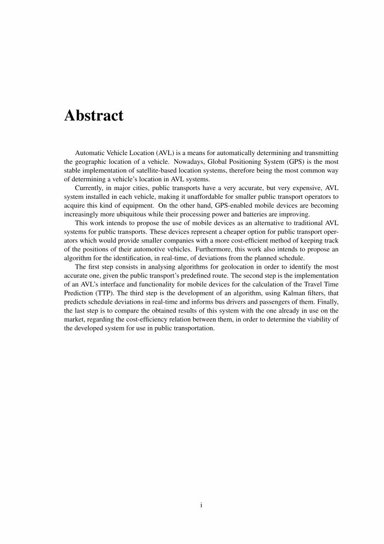
Abstract

Automatic Vehicle Location (AVL) is a means for automatically determining and transmittingthe geographic location of a vehicle. Nowadays, Global Positioning System (GPS) is the moststable implementation of satellite-based location systems, therefore being the most common wayof determining a vehicle’s location in AVL systems.

Currently, in major cities, public transports have a very accurate, but very expensive, AVLsystem installed in each vehicle, making it unaffordable for smaller public transport operators toacquire this kind of equipment. On the other hand, GPS-enabled mobile devices are becomingincreasingly more ubiquitous while their processing power and batteries are improving.

This work intends to propose the use of mobile devices as an alternative to traditional AVLsystems for public transports. These devices represent a cheaper option for public transport oper-ators which would provide smaller companies with a more cost-efficient method of keeping trackof the positions of their automotive vehicles. Furthermore, this work also intends to propose analgorithm for the identification, in real-time, of deviations from the planned schedule.

The first step consists in analysing algorithms for geolocation in order to identify the mostaccurate one, given the public transport’s predefined route. The second step is the implementationof an AVL’s interface and functionality for mobile devices for the calculation of the Travel TimePrediction (TTP). The third step is the development of an algorithm, using Kalman filters, thatpredicts schedule deviations in real-time and informs bus drivers and passengers of them. Finally,the last step is to compare the obtained results of this system with the one already in use on themarket, regarding the cost-efficiency relation between them, in order to determine the viability ofthe developed system for use in public transportation.

i

ii

Resumo

Localização Automática de Veículos (AVL) é um meio para determinar e transmitir a local-ização geográfica de um veículo automaticamente. Hoje em dia, o Sistema de PosicionamentoGlobal (GPS) é a implementação mais estável de sistemas de localização baseados em satélites,sendo, consequentemente, a forma mais comum de determinação de localização de um veículo emsistemas AVL.

Atualmente, nas grandes cidades, os transportes públicos têm um sistema AVL muito preciso,mas muito caro, instalado em cada veículo, tornando-o inviável para os pequenos operadores detransportes públicos para adquirir este tipo de equipamento. Por outro lado, os dispositivos móveiscom GPS estão a tornar-se cada vez mais presentes, enquanto o seu poder de processamento e asbaterias estão a melhorar.

Este trabalho pretende propor o uso de dispositivos móveis como uma alternativa aos sistemastradicionais AVL para transportes públicos. Estes dispositivos representam uma opção mais baratapara os operadores de transportes públicos, o que proporciona às pequenas empresas um métodomais eficiente, em termos de custo, de manter o controlo das posições dos seus veículos. Alémdisso, este trabalho também pretende propor um algoritmo para a identificação, em tempo real, dedesvios do cronograma planeado.

O primeiro passo consiste em analisar algoritmos para geolocalização, a fim de identificar omais preciso, dado um percurso predefinido do transporte público. O segundo passo é a imple-mentação de uma interface e funcionalidades de um AVL orientado a dispositivos móveis parao cálculo da Previsão do Tempo de Viagem (TTP). O terceiro passo é o desenvolvimento de umalgoritmo, usando filtros de Kalman, que prevê desvios no cumprimento do horário em tempo reale informa os motoristas de autocarros e passageiros destes desvios. Finalmente, a última etapa écomparar os resultados obtidos no presente sistema com o já em uso no mercado, no que respeita arelação custo-eficiência entre eles, a fim de determinar a viabilidade do sistema desenvolvido parao uso em transportes públicos.

iii

iv

Acknowledgements

First of all, I would like to thank my supervisor, Maria Teresa Galvão Dias, for the opportunitygranted to carry out this dissertation and the Sociedade de Transportes Coletivos do Porto (STCP)for all the data provided about bus routes and all the collaboration by the STCP bus drivers Iinteracted with when I was collecting the results for this dissertation.

To André Filipe Roque Silva, the one that never refused my requests for help and answeredmy doubts. I just wish I had your talent with words just to be able to meet your expectations.

To my parents and friends that kept motivating me to achieve my goals and to that unique onethat was able to give me the last push, the last strength, with a simple game, a simple challenge,but a lot of trust and expectations, I give you my sincere appreciation because this is all becauseof you.

Lastly, to the most important person, the brother life gave me, the one and only capable ofspending days and nights of invaluable help and effort, to you, Victor Filipe Carneiro Cerqueira, Igive you not only my greatest and truly word of appreciation but I give you my word that, whenyour time comes, I’ll be there wasting my life like you wasted yours. Because by wasting my lifein this way, I’ll be doing exactly the opposite: I’ll be able to finally be closer to reward everythingyou did for me. It’s not a matter of being rigorous with debts, it’s just a huge wish to be there foryou like you were for me. And if, by any chance, you don’t need any help, I’ll just be there to takeyou a coffee and put some jazz to help you to focus. You can always count on me.

Cristiano Seabra

v

vi

“I see now that the circumstances of one’s birth are irrelevant.It is what you do with the gift of life that determines who you are.”

Takeshi Shudo

vii

viii

Contents

1 Introduction 11.1 Context . . . . . . . . . . . . . . . . . . . . . . . . . . . . . . . . . . . . . . . 11.2 Motivation and Goals . . . . . . . . . . . . . . . . . . . . . . . . . . . . . . . . 11.3 Structure of this document . . . . . . . . . . . . . . . . . . . . . . . . . . . . . 2

2 Literature Review 32.1 Introduction . . . . . . . . . . . . . . . . . . . . . . . . . . . . . . . . . . . . . 32.2 Intelligent transportation systems (ITS) . . . . . . . . . . . . . . . . . . . . . . 3

2.2.1 Global Positioning System (GPS) . . . . . . . . . . . . . . . . . . . . . 42.2.2 Automatic Vehicle Location (AVL) . . . . . . . . . . . . . . . . . . . . 6

2.3 Travel Time Prediction (TTP) . . . . . . . . . . . . . . . . . . . . . . . . . . . . 92.3.1 Kalman filter . . . . . . . . . . . . . . . . . . . . . . . . . . . . . . . . 11

2.4 Relevant Projects and Research . . . . . . . . . . . . . . . . . . . . . . . . . . . 112.5 Conclusions . . . . . . . . . . . . . . . . . . . . . . . . . . . . . . . . . . . . . 12

3 SAE Light Controller 133.1 Introduction . . . . . . . . . . . . . . . . . . . . . . . . . . . . . . . . . . . . . 133.2 Architecture . . . . . . . . . . . . . . . . . . . . . . . . . . . . . . . . . . . . . 133.3 Data collection methodology . . . . . . . . . . . . . . . . . . . . . . . . . . . . 143.4 Major challenges and risks . . . . . . . . . . . . . . . . . . . . . . . . . . . . . 153.5 Conclusions . . . . . . . . . . . . . . . . . . . . . . . . . . . . . . . . . . . . . 16

4 Implementation 174.1 Kalman filters . . . . . . . . . . . . . . . . . . . . . . . . . . . . . . . . . . . . 19

4.1.1 Constructor . . . . . . . . . . . . . . . . . . . . . . . . . . . . . . . . . 214.1.2 Apply Kalman filter . . . . . . . . . . . . . . . . . . . . . . . . . . . . 22

4.2 Conclusion . . . . . . . . . . . . . . . . . . . . . . . . . . . . . . . . . . . . . 23

5 Test results and analysis 255.1 Collected results . . . . . . . . . . . . . . . . . . . . . . . . . . . . . . . . . . . 255.2 Results’ analysis . . . . . . . . . . . . . . . . . . . . . . . . . . . . . . . . . . 26

6 Conclusion and Future Work 33

References 35

ix

CONTENTS

x

List of Figures

2.1 GPS triangulation process . . . . . . . . . . . . . . . . . . . . . . . . . . . . . . 52.2 Brief explanation of location tracking . . . . . . . . . . . . . . . . . . . . . . . 6

3.1 Planned architecture for SAE Light Controller . . . . . . . . . . . . . . . . . . . 14

4.1 SAE Light Controller Main Activity screen . . . . . . . . . . . . . . . . . . . . 184.2 SAE Light Controller Google Maps activity screen . . . . . . . . . . . . . . . . 194.3 SAE Light Controller Google Maps position and last stored position difference . 20

5.1 Route 301 positions recorded for two different bus trips . . . . . . . . . . . . . . 265.2 Route 401 positions recorded for two different bus trips, with different directions 275.3 Estimation errors for the first trip of route 301 . . . . . . . . . . . . . . . . . . . 285.4 Comparison of arrival times for the first trip of route 301 . . . . . . . . . . . . . 285.5 Estimation errors for the second trip of route 301 . . . . . . . . . . . . . . . . . 295.6 Comparison of arrival times for the second trip of route 301 . . . . . . . . . . . . 295.7 Estimation errors of route 401 . . . . . . . . . . . . . . . . . . . . . . . . . . . 305.8 Comparison of arrival times of route 401 . . . . . . . . . . . . . . . . . . . . . . 305.9 Prediction errors of carried out bus trips . . . . . . . . . . . . . . . . . . . . . . 31

xi

LIST OF FIGURES

xii

List of Tables

xiii

LIST OF TABLES

xiv

Abbreviations

APC Automatic Passenger CountingAVL Automatic Vehicle LocationCDMA Code Division Multiple AccessFEUP Faculdade de Engenharia da Universidade do PortoGPS Global Positioning SystemGSM Global System for Mobile CommunicationsGSMPS Global System for Mobile Communications Positioning SystemITS Intelligent Transport SystemsRFID Radio Frequency IdentificationSTCP Sociedade de Transportes Coletivos do PortoTT Travel TimeTTP Travel Time PredictionUDP User Datagram ProtocolWPS Wi-Fi Positioning System

xv

Chapter 1

Introduction

1.1 Context

Intelligent Transport Systems (ITS) help drivers in carrying out their task. These bring advan-

tages, depending on their configuration, as the level of safety, comfort and ease of driving, always

ensuring that the final decision remains with the driver.

Global Positioning System (GPS) is a space-based navigation system, based on satellites, that

is widely used nowadays. These systems have a long history of use by maritime and aeronautical

transport, however recent GPS applications on land had several improvements, such system control

capabilities [MBP+04].

Automatic Vehicle Location (AVL) is a means for automatically determining and transmitting

the geographic location of a vehicle. The use of GPS-based AVL systems brought to the transit

industry and public transport companies an efficient way in performance and associated costs,

largely due to the fact that GPS systems are becoming cheaper and compact, in order to control

operations of their vehicles [PRM+10]. These ITS provide users with reliable and up-to-date

information such as time and location, i.e., how long the vehicle will take to reach the desired

destination, or the location where the vehicle is at any given time. This capability is important

because it attracts more users to attend these public transport and help to better plan their transit

and multimodal trip itineraries and allows them to make better decisions before and during the use

of public transports.

1.2 Motivation and Goals

The cost of AVL devices presents a significant investment, which mainly affects the develop-

ment of small and medium-sized public transportation companies.

Therefore, this work will focus on the development of an application capable of performing

the functionality of an AVL system based on GPS to calculate Travel Time Prediction (TTP),

capable of running on an Android mobile device, since such a measure would provide a low-cost

alternative to existing AVL devices. At the same time, these features will be analysed for the

1

Introduction

cost-benefit relation, as it is important to maintain a level of reliability and accuracy, considered

adequate, to the operational requirements of the public transport networks in the current context.

It will also be analysed the fulfilment of the time schedule in order to inform the driver and the

users of the vehicle’s relative position within the preset timetable.

1.3 Structure of this document

Besides this introductory chapter, this document contains 3 more chapters. In chapter 2 we

review the existing literature on the topic and present some related works. After that, in chapter 3,

we present the idea and potential of SAE Light Controller, as well the methodology planned and

major challenges. In chapter 4 we present how we implemented our solution, as well as the chosen

design and the necessary requirements for its operation. In chapter 5 we present and explain the

obtained results and discuss these to verify the successfulness of our solution in the context of our

problem. Lastly, in chapter 6 we conclude this dissertation about AVL systems and introduce some

future work to possibly obtain more accurate results in the calculation of TTP and some features

for the deployment of SAE Light Controller on the market.

2

Chapter 2

Literature Review

2.1 Introduction

This chapter aims to map out some work previously performed in the area of Intelligent Trans-

portation Systems (ITS), the use of Automatic Vehicle Location (AVL) systems and use of algo-

rithms for increased data accuracy.

At the time of writing, there are several works done by researchers in these areas and that

allows us to have a solid basis for the preparation of this work. This solid foundation provides us

the best way to solve the problem and therefore drawing important conclusions that are present in

the last section of this chapter.

2.2 Intelligent transportation systems (ITS)

Transportation flows are more and more monitored and controlled with systems of diverse

technologies. However, it proves difficult to visualize the data generated by travelling. Therefore,

it may be difficult to visualize how others might be interpreting, sharing and responding to these

data, and how individual or automated reactions to these data will modify mobilities or experiences

[Mon07]. For this reason, ITS have been deployed around the world, mostly in major cities.

Intelligent Transportation Systems (ITS) are advanced applications comprised by a hetero-

geneous network of technologies for highways and roads. These applications aim to provide

innovative services relating to different modes of transport and traffic management, without intel-

ligence as such. Because of this, ITS make safer, more coordinated and "smarter" use of transport

networks.

The main advantage of using ITS with transport networks is the translation of transportation

flows into data that can be used, if possible in real-time, through predictive modelling [Mon07].

Also, ITS allows to obtain very useful data for purposes of efficiency, security and commercial

marketing. Some examples are:

• In public transportation, GPS can be used to track the exact location of trains and buses;

3

Literature Review

• Smart cards embedded with radio frequency identification (RFID) allow for automated elec-

tronic payment for the use of highways and bridges;

• License-plated recognition systems are deployed to minimize traffic congestion and assess-

ing fines;

• Systems for in-car utilisation, such as black boxes, GPS units, or vehicle-to-vehicle com-

munication technologies, allow an increased inspection by insurance companies, marketers,

rental car agencies, law enforcement and others.

Although GPS localization and Automatic Passenger Counting (APC) are the most popular in-

formation to be obtained by automated data collection systems from on-board sensors, Moreira-

Matias et al [MMMMdSG15] presents other potentially valuable data items in his work:

• Stop and start moment: by recording when the vehicle starts and stops, information regard-

ing dwell time (the amount of time the vehicle is in a given state) and holding (the amount

of time spent at a stop) can be obtained.

• Event codes: these range from automated mechanical alarms or flags to manually entered

alarms.

• Control messages: through the establishment of a communication channel from the control

centre to the operator, messages reporting the corrective actions necessary to restore service

normality after it has deviated can be sent.

• Farebox transactions: by recording information about ticket validation (especially its type),

statistics about the passengers served by a given route can be calculated. This is helpful in

many planning and control tasks, including maintenance scheduling, route designing and

timetabling, corrective control actions and route designing. Due to this, these types of data

items are already deployed in many AVL systems worldwide.

2.2.1 Global Positioning System (GPS)

Global Positioning System (GPS) is a satellite positioning system, composed of a network of

27 or more satellites that orbit the Earth, that provides information about position, accurate timing

and velocity [TYK05], regardless of atmospheric conditions, time of day or location, as long as

the receiver finds at least three GPS satellites in his/her field of view. By making use of four or

more satellites, the accuracy of the measurements can be increased.

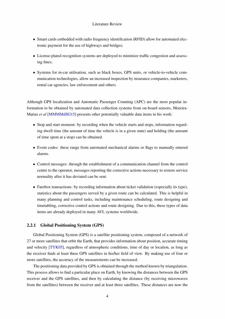
The positioning data provided by GPS is obtained through the method known by triangulation.

This process allows to find a particular place on Earth, by knowing the distances between the GPS

receiver and the GPS satellites, and then by calculating the distance (by receiving microwaves

from the satellites) between the receiver and at least three satellites. These distances are now the

4

Literature Review

radii on three separate spheres and the location that is to be calculated is derived from the point at

which the three spheres intersect [TYK05], as shown in Figure 2.11.

Figure 2.1: GPS triangulation process

Nowadays, due to its reliability and availability, GPS is considered the most efficient vehicle

locating method, and is the most widely implemented one [PRM+10]. Even in more remote areas,

the advances made regarding the sensitivity of GPS receivers allows them to work reliably. This

contrasts to other locating methods, such as Radio Frequency Identification (RFID), which pose

significant set-up costs related to the deployment and maintenance of the complete network of

sensors and power supplies that providing a monitoring service based on them would require.

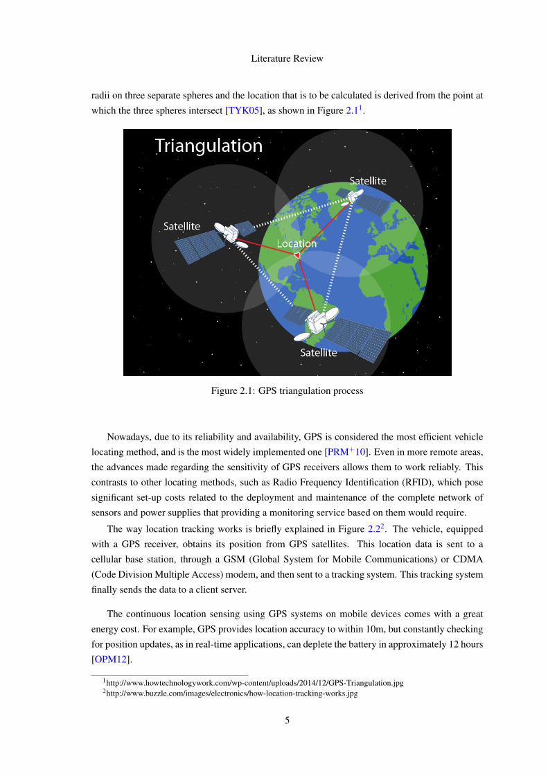
The way location tracking works is briefly explained in Figure 2.22. The vehicle, equipped

with a GPS receiver, obtains its position from GPS satellites. This location data is sent to a

cellular base station, through a GSM (Global System for Mobile Communications) or CDMA

(Code Division Multiple Access) modem, and then sent to a tracking system. This tracking system

finally sends the data to a client server.

The continuous location sensing using GPS systems on mobile devices comes with a great

energy cost. For example, GPS provides location accuracy to within 10m, but constantly checking

for position updates, as in real-time applications, can deplete the battery in approximately 12 hours

[OPM12].

1http://www.howtechnologywork.com/wp-content/uploads/2014/12/GPS-Triangulation.jpg2http://www.buzzle.com/images/electronics/how-location-tracking-works.jpg

5

Literature Review

Figure 2.2: Brief explanation of location tracking

However, smartphones are equipped with real-time sensing and user activity recognition by

using, for example, very common sensors such as accelerometers, and other alternatives for loca-

tion sensing technologies such as Wi-Fi Positioning System (WPS) and Global System for Mobile

Communications Positioning System (GSMPS). Nevertheless, the biggest problem of using WPS

and GSMPS for improving the energy-efficiency of GPS is the increased average localization error.

The location accuracy, in urban areas, for WPS and GSMPS are approximately 20-30m and 70-

200m respectively [OPM12], which may prove to be very difficult to use in real-time applications

that need to have accurate results to achieve their goals.

2.2.2 Automatic Vehicle Location (AVL)

Automatic Vehicle Location (AVL) is a means for automatically obtaining and transmitting

the geolocation of a vehicle to an appropriate tracking system in order to provide an overview of

its travel pattern.

Automatic vehicle locating is commonly used for managing fleets of vehicles, be they service

vehicles, emergency vehicles, precious construction equipment, or public transport vehicles (buses

and trains). It is also used to track mobile assets, such as non wheeled construction equipment,

non motorized trailers, and mobile power generators.

With the increase in traffic congestion and, therefore, passenger demands, many public trans-

port operators seek to improve their operations by investing in this technology, which holds sub-

stantial promise for improving service planning, timetable scheduling and performance analysis

practices [FHMS03].

Today’s bus AVL systems include the core location tracking capabilities and other additional

functionalities, with some obtained through other sensors and devices in the bus, such as [Par08]:

• Text messaging data communications between operators and dispatch;

6

Literature Review

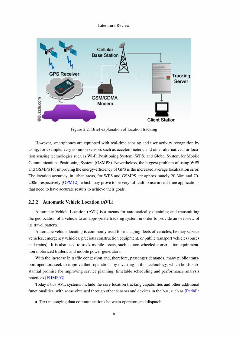
Figure 2.3: Display in a London’s bus

• Manager of headsign and farebox;

• Onboard next stop announcements that are automatically triggered as the vehicle approaches

the stop, by voice and/or displays (such as Figure 2.33);

• Onboard automatic passenger counting (APC) equipment to record the number of passen-

gers boarding;

• Show some vehicle’s monitor status messages;

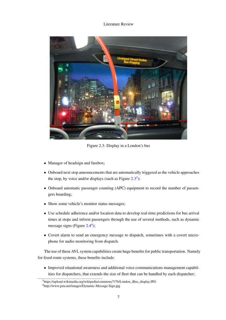
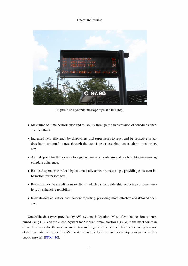
• Use schedule adherence and/or location data to develop real-time predictions for bus arrival

times at stops and inform passengers through the use of several methods, such as dynamic

message signs (Figure 2.44);

• Covert alarm to send an emergency message to dispatch, sometimes with a covert micro-

phone for audio monitoring from dispatch.

The use of these AVL system capabilities create huge benefits for public transportation. Namely

for fixed-route systems, these benefits include:

• Improved situational awareness and additional voice communications management capabil-

ities for dispatchers, that extends the size of fleet that can be handled by each dispatcher;3https://upload.wikimedia.org/wikipedia/commons/7/76/London_iBus_display.JPG4http://www.psta.net/images/Dynamic-Message-Sign.jpg

7

Literature Review

Figure 2.4: Dynamic message sign at a bus stop

• Maximize on-time performance and reliability through the transmission of schedule adher-

ence feedback;

• Increased help efficiency by dispatchers and supervisors to react and be proactive in ad-

dressing operational issues, through the use of text messaging, covert alarm monitoring,

etc;

• A single point for the operator to login and manage headsigns and farebox data, maximizing

schedule adherence;

• Reduced operator workload by automatically announce next stops, providing consistent in-

formation for passengers;

• Real-time next bus predictions to clients, which can help ridership, reducing customer anx-

iety, by enhancing reliability;

• Reliable data collection and incident reporting, providing more effective and detailed anal-

ysis.

One of the data types provided by AVL systems is location. Most often, the location is deter-

mined using GPS and the Global System for Mobile Communications (GSM) is the most common

channel to be used as the mechanism for transmitting the information. This occurs mainly because

of the low data rate needed by AVL systems and the low cost and near-ubiquitous nature of this

public network [PRM+10].

8

Literature Review

AVL output consists of an array of points in time and two dimensional space, representing a set

of coordinates at a given timestamp. This form of location data is well suited for vehicle location

visualization on a map or for determining whether a certain vehicle is following its assigned route.

Furthermore, the coordinates in this array can be transformed into a single value representing

the distance between the current position and the next stop in the vehicle’s route. This transfor-

mation leads to a shift from a three dimensional problem (latitude, longitude and time) to a two

dimensional problem (time and one spatial dimension), which is easier to compute.

2.3 Travel Time Prediction (TTP)

Moreira-Matias et al define Travel Time Predictions (TTP) as one of the most common prob-

lems in transportation [MMMMdSG15].

As stated by Lin et al, being able to receive, from traveller information systems, information

on bus arrival time at bus stops could reduce the anxiety of passengers waiting for the bus [LZ99].

Message signs or applications displaying this information are being used right now in major cities

around the globe, helping to improve the reliability and effectiveness of traveller information ser-

vices and commuters’ satisfaction with the service offered. AVL, frequently presented as a source

of a vehicle’s position information, produces data suitable for obtaining arrival time predictions

[PRM+10].

TTP can be used in several other contexts besides fleet management, such as logistics, indi-

vidual navigation or mass transit, planning, monitoring, and control. Although some approaches

seem quite simple, there are various methodologies that could be applied to TTP problems from

different research areas. Moreira-Matias divides these approaches into four different categories

[MMMMdSG15]:

• Machine Learning and Regression Methods: these methods make use of a mathematical

function based on a set of independent variables to infer the arrival time (the dependent

variable). Regression models have been the state of the art on this kind of approach for

the last two decades. These methods are mainly used to estimate and plan the timetable

schedule of a public transport and not used for real-time analysis.

• State-Based and Time Series Models: these methods only take into account the most recent

data samples, and thus do not depend as much on the amount of data, nor do they require

a large training period, as they mainly represent online learning algorithms. This ability to

learn and update in real-time makes them able to react well to unexpected events that may

affect the expected traffic flow, such as heavy rains, traffic jams, sports matches, and car ac-

cidents. While the time series models assume that the Travel Time (TT) is a linear/nonlinear

combination of its historical values, the state-based approaches usually assume that the fu-

ture state of the dependent variables only relies on the most recent states. The most popular

state-based model is the Kalman filter. The main advantage of this model when compared

9

Literature Review

with Markovian approaches is its ability to filter noise in the data, which is extremely rele-

vant in online learning tasks for short-term prediction problems.

• Flow Conservation Equations and Traffic Dynamics Models: these methods focus on formu-

lating the Travel Time (TT) between two points as a sum of the TT between smaller stretches

of the route being analysed (i.e., roads). This is done by applying relations between traffic

variables obtained from the traffic flow theory.

• On Evaluating TTP Models: these methods consist of simple averages and other types of

time-varying Poisson processes whose average Travel Time (TT) is defined by its historical

values depending on the day type and/or on the period of the day. Due to the simplicity of

these models, they are unable to represent complex relationships between the TT and other

variables present in urban public transport networks, and are therefore usually considered to

be a poor approach to TTP.

As stated in Moreira-Matias [MMMMdSG15], AVL systems and their large-sale introduction

in public transportation around the world created new opportunities to operational controllers and

made it possible to create highly sophisticated control centres to monitor all the vehicles in real-

time. However, this requires a large amount of human resources. By exploring the historical data

from AVL systems, researchers started to build automatic control strategies, which can maintain

the buses on schedule, while reducing the number of human resources needed in the process.

Therefore, some corrective actions have been employed as real-time control strategies:

• Bus holding: It consists of forcing the driver to increase, or decrease, the dwell time on a

bus stop along the route;

• Speed modification: This strategy consists of forcing the driver to reduce the maximum

cruise speed on its course, comparative to what’s usual on that specific route;

• Stop-skipping: When it is required to make a path change to reduce the original length of

the route, the driver must skip some route stops;

• Short-turning: This technique forces the driver to skip the remaining bus stops, usually at

its terminus, in order to fill a large gap in another route, sometimes forcing the passengers

to transfer to another transportation.

Bus holding strategies are the most classic way of keeping the bus on-schedule. However,

this strategies, as well as speed modification, are made by increasing the TT of the passengers in

the vehicle. Moreover, stop-skipping and short-turning strategies corrects the time schedule by

keeping the passengers waiting on the stops that were skipped [MMMMdSG15].

10

Literature Review

2.3.1 Kalman filter

As mentioned earlier, Kalman filters have emerged over time as a very reliable implementation

solution and are widely used by many researchers for the task of calculating the TTP for state-

based models, namely those intended for real-time use [MMMMdSG15].

The Kalman filter is a linear recursive predictive update algorithm invented in 1960 by Rudolf

Emil Kalman, that is used to estimate the parameters of a process model [Kal60].

From an engineering standpoint, it is normal to try to create linear mathematical models of

real systems. So, when these implicate non-linearity, it is logical to attempt to linearise the system

to an operating point. A linear system is easier to handle with existing mathematical tools and the

theory which supports these systems is much more complete and practical than the one supporting

nonlinear ones. Nonetheless, some systems are impossible to linearise, though there are variants

of the Kalman filter that specifically deal with nonlinear systems [May82].

As Predic et al stated, the Kalman filter’s ability to combine the effects of noise on both the

process and the measurements and the computationally manageable nature of its algorithms made

it very popular, namely in the areas of autonomous and assisted navigation [PRM+10].

It is important to note that as this filter was developed for treating linear systems, it can only

be an optimal state estimator if the system is linear and the noise of the process and the measures

are white and Gaussian [May82].

Past data used as input to the Kalman filter is collected from the previous bus runs, even on

the same day, and the accuracy of this input can increase by having past days’ data [PRM+10].

For the GPS’ implementations on mobile devices, the use of Kalman filters appears to vary

depending on the hardware used and the system’s implementation. There are, however, ways to

identify if a particular device implements these filters by analysing the system’s log output 5.

2.4 Relevant Projects and Research

Systems dealing with prediction problems in public transportation exist either as scientific

projects or as commercial solutions that have been implemented in many cities [PRM+10].

MYBUS (2001) is the result of a scientific project developed for ITS at the University of

Washington. A Kalman filter is used to stream location and velocity data for each bus and then

mapped to match the geometry of the route on which the bus is operating. This geometry is divided

into several smaller segments, in order to estimate the time the bus will take to arrive at the station.

This way, it is practicable to assume that the vehicle will be travelling at a constant speed on

each segment. In the end, the final estimated time is the sum of the calculated times per segment.

However, speed can change very easily because of the city’s traffic conditions unpredictability.

Therefore, predictions based solely on speed can be very unstable [PRM+10]. This is why Predic

et al state the usefulness of AVL systems based on GPS for obtaining the vehicle’s location and

5http://gis.stackexchange.com/questions/87182/what-class-types-of-smartphone-chipsets-support-gps-a-gps-glonass-and-have-ext

11

Literature Review

then estimate the time the bus will take to arrive the station, in a more dynamic way, using Kalman

filters.

Also, it is stated that Shalaby and Farhan (2004) compared their proposed method to other pre-

viously developed models and the use of Kalman filters exhibited better predictive performance in

the simulated environments, with dynamic changes due to different characteristics of bus opera-

tion. In addition to its performance, since the model separates the bus dwell time prediction from

the bus running time prediction, it has the advantage of capturing the effects of control strategies

[PRM+10]. This research deals with unpredictabilities in bus operations such as traffic accidents

and varying number of passengers boarding and leaving the bus at certain stops.

2.5 Conclusions

The literature proves the huge benefits of using AVL systems in public transportation. Their

accuracy and effectiveness improves the reliability and user experience, decreasing passenger’s

anxiety and increasing ridership. It’s a great tool for drivers, because it provides them useful

information, but even more for the companies that use this data for planning schedule updates,

new routes or service plans adapted to new circumstances.

Besides all the ITS functions implemented in public transportation, AVL’s basic function of

automatically locating a vehicle’s position, through the use of GPS, is extremely accurate due to

the fact that the GPS receiver used in AVL systems has Kalman filters implemented on. Therefore,

the use of Kalman filters in vehicle location is really important to reduce noise and maximize

accuracy in data gathering for the TTP and vehicle positioning on map. This focus on accuracy

and all the other functions that an AVL gathers, is what makes this kind of device excel and become

such a valuable tool for operators to acquire.

It is also stated in the literature that it is possible, through the use of state-based models and

Kalman filters, that the development of real-time applications of vehicle tracking and TTP calcu-

lation for time scheduling is possible. It is also stated that mobile devices do not pose a major

challenge to implement these applications on.

12

Chapter 3

SAE Light Controller

3.1 Introduction

Knowing about the utilisation of AVL systems in public transportation, as mentioned in the

previous chapter, we propose the development of SAE Light Controller.

SAE Light Controller is an application for mobile devices, namely those with the Android

operating system, in order to be a light and capable application to perform the functions of an

AVL system currently used in public transportation, in order to make it possible to acquire a mobile

device with the application, rather than purchasing expensive AVL systems, for the calculation of

the TTP.

This solution will automatically detect the vehicle’s location, velocity and travelled distance,

in real-time, and, by knowing the elapsed time, apply a Kalman filter to get the estimated arrival

time. This way, the drivers, using SAE Light Controller, will be able to control the time schedule,

just from looking at the mobile device, and know if the bus is ahead or behind schedule. This

process is automatic and the drivers only have to input the route’s number, direction and start time

and, after a button click, see their position on the map and the estimated arrival time.

The ultimate goal of this dissertation is to compare the performance of SAE Light Controller

with AVL systems currently used nowadays, to check if the cost reduction is sufficiently capable

to compete with these AVL systems.

3.2 Architecture

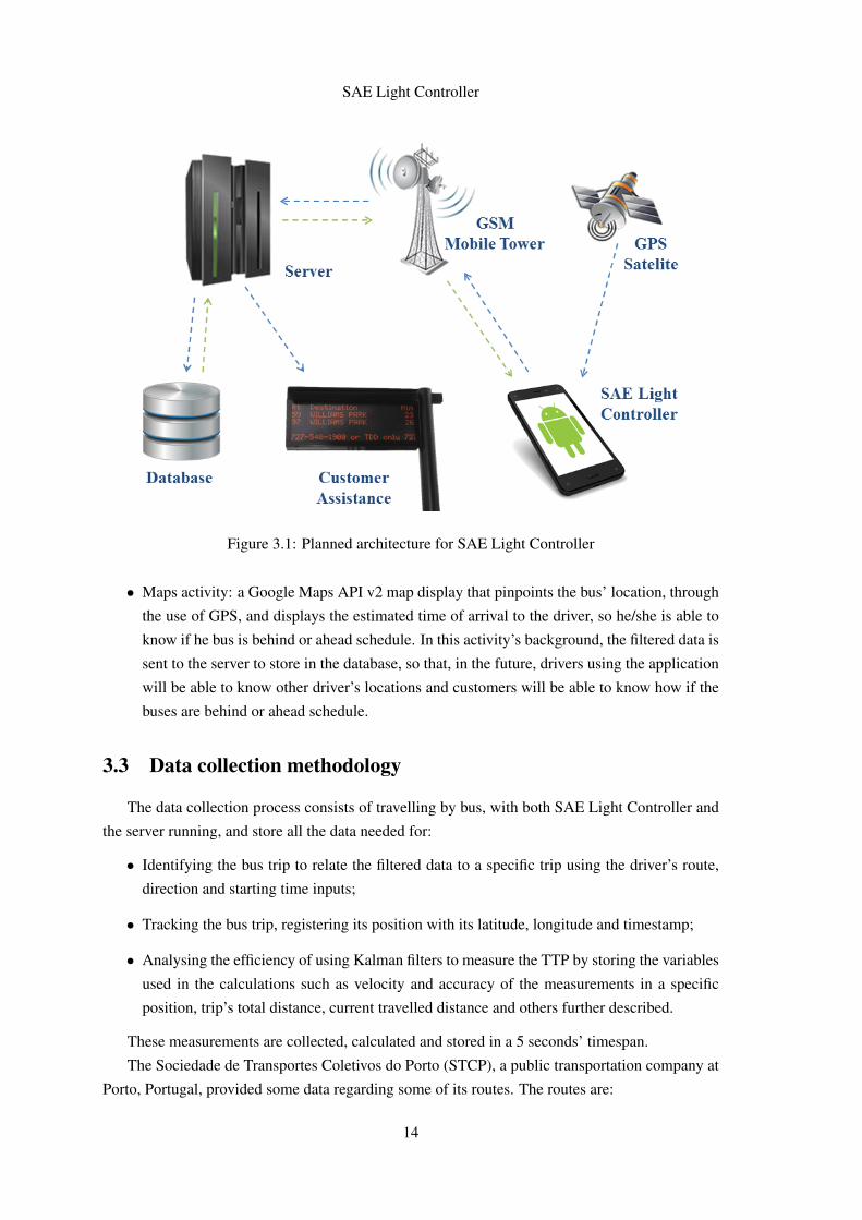
The implementation’s structure of the application is illustrated in Figure 3.1.

SAE Light Controller is composed of two different activities:

• Main activity: a simple screen, with only three input requirements for the driver to identify

the desired line trip. This data is sent to the server that will query the database, where the

route’s details are stored, and get the necessary data needed to apply the Kalman filters.

After this, the data is consequently sent to the Maps Activity.

13


Figure 3.1: Planned architecture for SAE Light Controller

• Maps activity: a Google Maps API v2 map display that pinpoints the bus’ location, through

the use of GPS, and displays the estimated time of arrival to the driver, so he/she is able to

know if he bus is behind or ahead schedule. In this activity’s background, the filtered data is

sent to the server to store in the database, so that, in the future, drivers using the application

will be able to know other driver’s locations and customers will be able to know how if the

buses are behind or ahead schedule.

3.3 Data collection methodology

The data collection process consists of travelling by bus, with both SAE Light Controller and

the server running, and store all the data needed for:

• Identifying the bus trip to relate the filtered data to a specific trip using the driver’s route,

direction and starting time inputs;

• Tracking the bus trip, registering its position with its latitude, longitude and timestamp;

• Analysing the efficiency of using Kalman filters to measure the TTP by storing the variables

used in the calculations such as velocity and accuracy of the measurements in a specific

position, trip’s total distance, current travelled distance and others further described.

These measurements are collected, calculated and stored in a 5 seconds’ timespan.

The Sociedade de Transportes Coletivos do Porto (STCP), a public transportation company at

Porto, Portugal, provided some data regarding some of its routes. The routes are:

14


• 301: A single direction circular bus trip around the city. As the provided route with the

biggest total distance, this one was tested 2 times. The scheduled start and end times of the

first bus trip were 10:00 a.m. and 11:14 a.m. respectively. The second bus trip started at

5:05 p.m and ended at 6:23 p.m..

• 401: A bidirectional bus trip between Bolhão and S. Roque. The direction "Volta", with

start in S. Roque, had to be discarded due to some road maintenance that diverted from the

original bus route, therefore not allowing the use of the data provided for that route. The

direction with starting point at Bolhão was tested 1 time.

Due to lack of time, only a total of 3 tests were made.

3.4 Major challenges and risks

The development and testing phases of SAE Light Controller may present some challenges

and risks and some of them could be already identified.

The identified challenges are:

• The main challenge of this dissertation is to provide a better cost-efficient alternative to AVL

systems. Therefore, it’s important to keep a competitive level of location, time and velocity

accuracy, compared to an existing AVL, to calculate a good estimate of arrival time and

make it viable to decrease the cost of the equipment.

• The battery level of the mobile device must not deplete while the public transport is working

actively. Because of the high GPS usage, the battery depletes fast, therefore the use of a

lighter charger is mandatory and enough to solve this problem.

• The type of data and how it is structured on the companies’ databases may prove to be

a challenge for the application to process. This poses a major challenge because if, for

example, the company has more detailed information about distances between stops the

algorithm can be highly improved.

• The testing phase needs some real-time field work, making the analyses much easier if some

cooperation is established with the companies, making it possible to execute more bus’ runs

and collect more data.

The identified risks are as follows:

• A continuous connection with GPS and Wi-Fi must be available because it’s crucial for

transmitting and receiving data and therefore obtain good results.

• The databases with public transportation lines and timetables may differ between compa-

nies, making the current implementation incapable of working thanks to the specific queries

to the database.

15


• The driver of the public transport should make the right inputs. Otherwise, it may lead the

application to work with wrong lines and/or time schedules because it doesn’t identify the

right route, it chooses another route or it simply isn’t capable to connect to server.

3.5 Conclusions

SAE Light Controller focuses on the consequences of using an AVL in the detection of a

vehicle’s location, analysis of compliance with the timetable and the processing and visualisation

of these data, to improve the experience of drivers and users of public transports, trying to maintain

a competitive data accuracy in calculating the travel time prediction.

In this chapter we detailed some features of SAE Light Controller as well as some of the risks

and challenges that had to face and some that the future may pose to the current implementation.

However, some of these challenges have simple solutions as we stated. For instance, the bat-

tery level of a smartphone depletes in approximately 12 hours of continuous requests for location

updates [OPM12] and this time can be increased with the use of a battery charger connected to the

bus itself. Also, the accuracy level of location and time prediction is possible to be acquired if the

company provides complete and descriptive data, mainly related to distances and estimated time

between bus’ stops.

Some of the risks appointed in previous sections may also prove little to nothing. GPS connec-

tion may be quite difficult in the countryside but in urban areas it is very effective. Also, nowadays

a huge portion of public transportation are equipped with Wi-Fi connection, for the application to

transmit data to the server. Finally, the planned interface for SAE Light Controller will be as

simple as possible, to minimize possible input errors from the driver; these inputs will be really

important to specify which route the bus will traverse, so the trip can be correctly identified for the

algorithm to work as it is expected.

16

Chapter 4

Implementation

SAE Light Controller is a mobile application for Android devices, with Android 4.4 (KitKat)

minimum version required, with a client-server architecture. The communication protocol be-

tween the client, developed in Java for Android, and the server, developed in Java, is UDP (User

Datagram Protocol). This protocol was chosen because it’s simple, fast and the possibility to lose

some data does not present a problem because the readings and calculations are made with a 5

seconds’ timespan and for the TTP calculation, after receiving the data from the server, the appli-

cation does not require Internet connectivity. Internet connectivity is only needed to identify the

route, get some related data from the database, track the bus’ positions through time and close the

running thread when the trip ends.

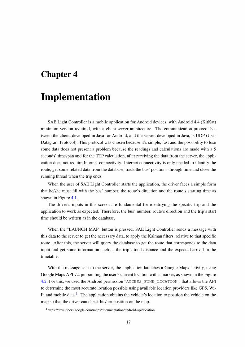
When the user of SAE Light Controller starts the application, the driver faces a simple form

that he/she must fill with the bus’ number, the route’s direction and the route’s starting time as

shown in Figure 4.1.

The driver’s inputs in this screen are fundamental for identifying the specific trip and the

application to work as expected. Therefore, the bus’ number, route’s direction and the trip’s start

time should be written as in the database.

When the "LAUNCH MAP" button is pressed, SAE Light Controller sends a message with

this data to the server to get the necessary data, to apply the Kalman filters, relative to that specific

route. After this, the server will query the database to get the route that corresponds to the data

input and get some information such as the trip’s total distance and the expected arrival in the

timetable.

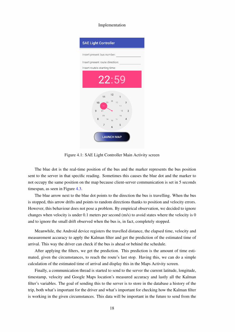
With the message sent to the server, the application launches a Google Maps activity, using

Google Maps API v2, pinpointing the user’s current location with a marker, as shown in the Figure

4.2. For this, we used the Android permission ”ACCESS_FINE_LOCATION", that allows the API

to determine the most accurate location possible using available location providers like GPS, Wi-

Fi and mobile data 1. The application obtains the vehicle’s location to position the vehicle on the

map so that the driver can check his/her position on the map.

1https://developers.google.com/maps/documentation/android-api/location

17

Implementation

Figure 4.1: SAE Light Controller Main Activity screen

The blue dot is the real-time position of the bus and the marker represents the bus position

sent to the server in that specific reading. Sometimes this causes the blue dot and the marker to

not occupy the same position on the map because client-server communication is set in 5 seconds

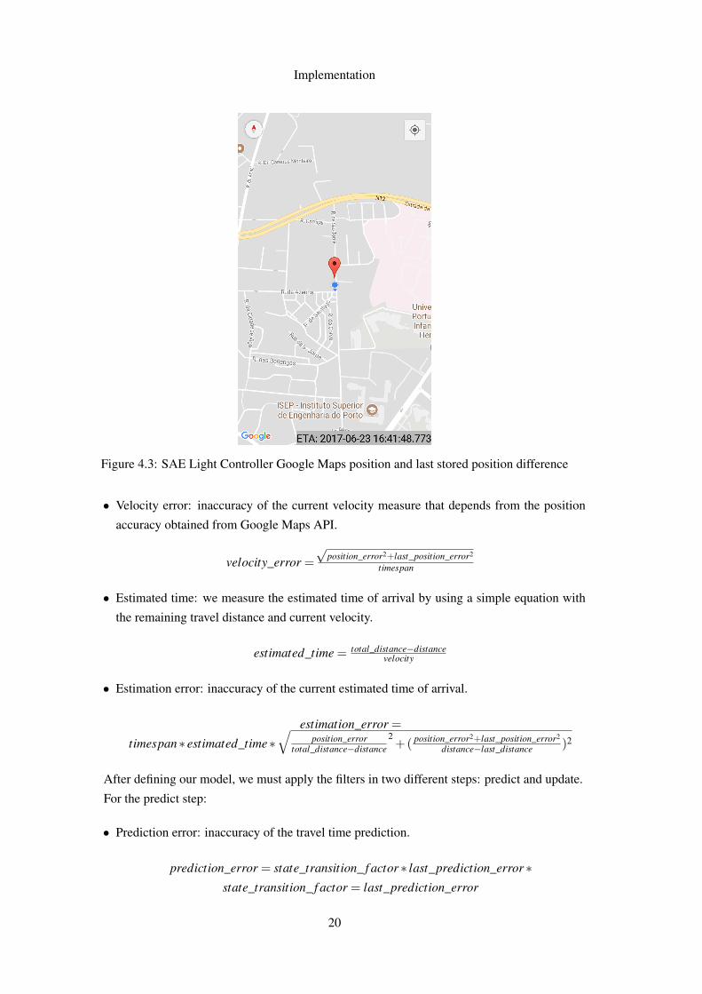
timespan, as seen in Figure 4.3.

The blue arrow next to the blue dot points to the direction the bus is travelling. When the bus

is stopped, this arrow drifts and points to random directions thanks to position and velocity errors.

However, this behaviour does not pose a problem. By empirical observation, we decided to ignore

changes when velocity is under 0.1 meters per second (m/s) to avoid states where the velocity is 0

and to ignore the small drift observed when the bus is, in fact, completely stopped.

Meanwhile, the Android device registers the travelled distance, the elapsed time, velocity and

measurement accuracy to apply the Kalman filter and get the prediction of the estimated time of

arrival. This way the driver can check if the bus is ahead or behind the schedule.

After applying the filters, we get the prediction. This prediction is the amount of time esti-

mated, given the circumstances, to reach the route’s last stop. Having this, we can do a simple

calculation of the estimated time of arrival and display this in the Maps Activity screen.

Finally, a communication thread is started to send to the server the current latitude, longitude,

timestamp, velocity and Google Maps location’s measured accuracy and lastly all the Kalman

filter’s variables. The goal of sending this to the server is to store in the database a history of the

trip, both what’s important for the driver and what’s important for checking how the Kalman filter

is working in the given circumstances. This data will be important in the future to send from the

18

Implementation

Figure 4.2: SAE Light Controller Google Maps activity screen

server to public transportation customers by some online platform, application, dynamic message

signs at bus’ stops and so on and to be able to analyse the collected results for this dissertation.

4.1 Kalman filters

As mentioned in the literature review, the Kalman filter is a linear recursive predictive update

algorithm and a very reliable implementation solution for calculating the TTP, namely for real-

time use. Our algorithm is composed by a constructor, to initialize some variables, and an apply

method, to calculate the estimated time prediction.

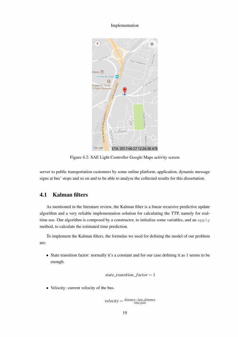
To implement the Kalman filters, the formulas we used for defining the model of our problem

are:

• State transition factor: normally it’s a constant and for our case defining it as 1 seems to be

enough.

state_transition_ f actor = 1

• Velocity: current velocity of the bus.

velocity = distance−last_distancetimespan

19

Implementation

Figure 4.3: SAE Light Controller Google Maps position and last stored position difference

• Velocity error: inaccuracy of the current velocity measure that depends from the position

accuracy obtained from Google Maps API.

velocity_error =√

position_error2+last_position_error2

timespan

• Estimated time: we measure the estimated time of arrival by using a simple equation with

the remaining travel distance and current velocity.

estimated_time = total_distance−distancevelocity

• Estimation error: inaccuracy of the current estimated time of arrival.

estimation_error =

timespan∗ estimated_time∗√

position_errortotal_distance−distance

2+( position_error2+last_position_error2

distance−last_distance )2

After defining our model, we must apply the filters in two different steps: predict and update.

For the predict step:

• Prediction error: inaccuracy of the travel time prediction.

prediction_error = state_transition_ f actor ∗ last_prediction_error ∗state_transition_ f actor = last_prediction_error

20

Implementation

• Prediction: travel time prediction; note that the control signal of our model is the elapsed

timespan and its factor is -1, therefore the TTP is expected to decrease over time.

prediction = state_transition_ f actor ∗ last_prediction+ control_signal_ f actor ∗control_signal = last_prediction− timespan

And for the update step:

• Gain: tradeoff between estimation and prediction.

gain = predictionprediction+estimation_error

• Updated prediction: applying the gain, the travel time prediction is updated.

updated_prediction = prediction+gain∗ (estimated_time− prediction)

• Prediction error: updates the inaccuracy of the travel time prediction.

prediction_error = (1−gain)∗ prediction_error

Having this knowledge present, it is possible to implement a Kalman filter class for calcu-

lating the TTP of a bus’ trip. The implemented algorithm follows strictly what is described on

constructor and apply further subsections of this chapter.

4.1.1 Constructor

The Kalman filter class constructor is called in Maps Activity on the onCreate method. The

constructor’s parameters are:

• Total distance: Trip’s total distance, measured in meters, through the use of Google Maps.

When the driver specifies he desired route, we know the its total distance in meters.

• Prediction error: This value, between 0 and 1, should not be 0 otherwise it will remain 0

forever. This value is updated every 5 seconds’ timespan, tending to a fixed value, and it is

related to the device. Every time the bus’ trip ends, the last value is stored in the device.

• Estimated time: Difference between the end and starting times, in milliseconds, of the spec-

ified bus trip.

The constructor initializes the Kalman filter’s object with these described values. It also ini-

tializes the current travelled distance as 0 meters and the updated prediction variable with the

estimated time, because, in the first iteration of the algorithm, the TTP is the scheduled in the bus’

timetable. All these values are necessary, as described in this chapter, to run the Kalman filter

algorithm.

21

Implementation

4.1.2 Apply Kalman filter

The Kalman filter class applymethod is called in Maps Activity on the onLocationChanged

method. This method is the one to really initialize he Kalman filter algorithm. The method’s pa-

rameters are:

• Timespan: difference between the current timestamp and the last measured location’s times-

tamp, that is, the elapsed time between 2 consecutive readings.

• Distance: Length between current location and last measured location.

• Velocity: Current bus’ travelling speed, in meters per second.

• Position error: Current Google Maps API v2 location’s measured accuracy, in meters.

The apply method sums to the current travelled distance with the received distance parame-

ter. Then, this method firstly calls calculateError, secondly predict and finally update,

consequently returning the TTP. All these methods will set the variables for each other, so that

the apply method, before returning, has the TTP, for that iteration, calculated and ready to be

displayed on the map for the driver to consult.

4.1.2.1 Calculate Error

The Kalman filter algorithm method calculateError is called on the apply method. This

method’s parameters are the same as the apply method, besides distance. This new distance

parameter is the current travelled distance, updated in the beginning of the apply method.

Firstly, it calculates the velocity error, as described earlier in this chapter, and, after this, if the

bus’ current velocity is under 0.1 meters per second, then the function ends, otherwise it updates

the Kalman filter object’s estimation error for the current state. The estimation error is calculated

as described earlier in this chapter, using timespan, estimated time, position error, last iteration’s

position error, current travelled distance and last iteration’s travelled distance.

4.1.2.2 Predict

The Kalman filter class predict method is called on the apply method. This method’s

parameters are timespan and velocity like the apply method.

Firstly, this function updates the mobile device’s prediction error, as described earlier in this

chapter, and, if velocity is below 0.1 meters per second, then the function ends, otherwise it calcu-

lates the prediction, also as described earlier.

4.1.2.3 Update

The Kalman filter class update method is called on the apply method. This method’s pa-

rameter is velocity like the apply method.

22

Implementation

If the bus current velocity is below 0.1 meters per second, it defines the Kalman filter’s gain as

0, otherwise the function calculates the gain and the estimated time for arrival. Then, the function

updates the prediction or, in other words, the TTP, using the calculated gain and estimated time,

and finally updates the prediction error value. Note that the calculation of gain, estimated time,

travel time prediction and prediction error are earlier described in this chapter.

4.2 Conclusion

The main challenge of this implementation was to define our model, so the problem can be

linearised for us to be able to apply a Kalman filter in each state to calculate the TTP. After we

defined our model, we are ready to apply the Kalman filter by calling predict and update. On

the predict step we simply update the values of the prediction and its error and, on the update step,

we use these values to calculate the gain. The gain is what measures if, in this step, the estimated

prediction is relevant. Then, we update the prediction error having the gain in mind: if the gain

tends to 0, the prediction error tends to be unchanged.

The prediction error is stored locally on the device because it is influenced by the device’s GPS

accuracy. By saving this value, knowing that, in the Kalman filter algorithm, the prediction error

tends to stabilize, the application is able to start calculating the TTP accurately from the route’s

start and do not have to wait for it to stabilize every bus’ trip.

It is also important to note that, if the bus is stopped the velocity will be equal or approximately

0, thanks to the velocity error, calculated using the position error. If this happens, that is, when

the velocity is under 0.1 meters per second, the prediction keeps unchanged and the gain is 0,

therefore the estimated prediction prevails, ignoring some position drift.

23

Implementation

24

Chapter 5

Test results and analysis

For the implementation and testing phases, the public transportation company STCP (So-

ciedade de Transportes Coletivos do Porto) provided some data about 3 different bus routes: 301,

401 and 806. Route 301 is a bus with a circular trajectory around the city and both 401 and 806

routes are buses with 2 different direction trajectories. Unfortunately, because the provided data

did not include weekend routes, we did not have the time needed to test route 806 or to collect

more data from the other routes.

With this provided data and at the time of testing, we did real-time field testing for only routes

301 and 401. One of the directions of route 401 was modified thanks to some street construction

works, therefore it is impossible to analyse the results for that specific trip in the temporarily

modified direction and, for data consistency, we collected data for 2 runs of route 301.

The Android device we used for collecting data was a Xiaomi Redmi 3s that we used for our

bus runs.

5.1 Collected results

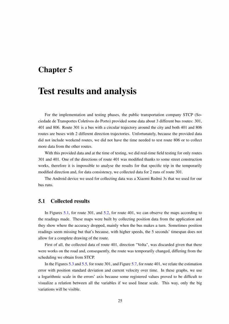
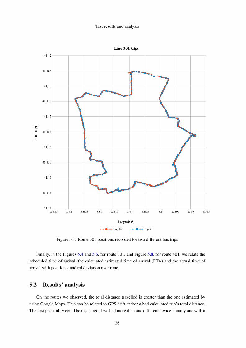
In Figures 5.1, for route 301, and 5.2, for route 401, we can observe the maps according to

the readings made. These maps were built by collecting position data from the application and

they show where the accuracy dropped, mainly when the bus makes a turn. Sometimes position

readings seem missing but that’s because, with higher speeds, the 5 seconds’ timespan does not

allow for a complete drawing of the route.

First of all, the collected data of route 401, direction "Volta", was discarded given that there

were works on the road and, consequently, the route was temporarily changed, differing from the

scheduling we obtain from STCP.

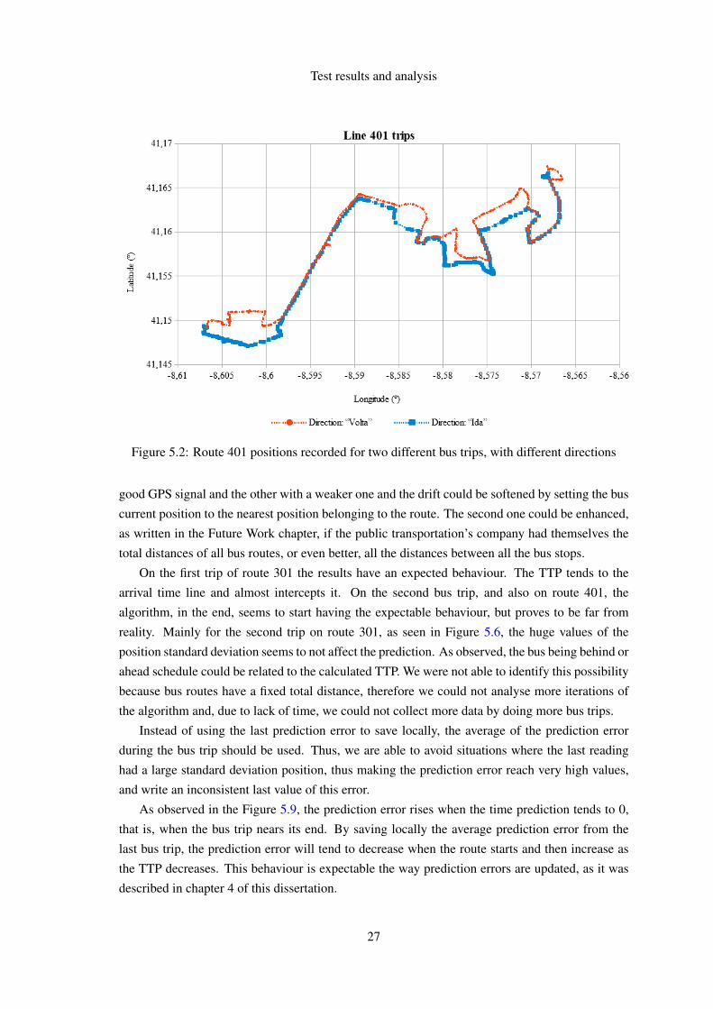
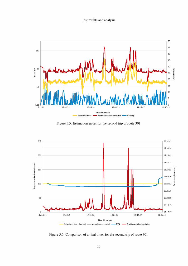
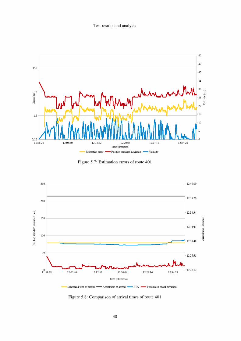
In the Figures 5.3 and 5.5, for route 301, and Figure 5.7, for route 401, we relate the estimation

error with position standard deviation and current velocity over time. In these graphs, we use

a logarithmic scale in the errors’ axis because some registered values proved to be difficult to

visualize a relation between all the variables if we used linear scale. This way, only the big

variations will be visible.

25


Figure 5.1: Route 301 positions recorded for two different bus trips

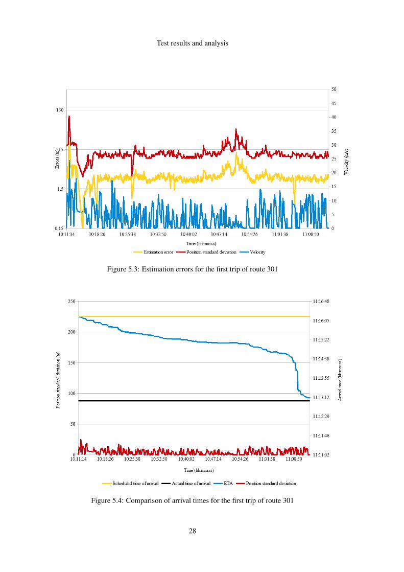
Finally, in the Figures 5.4 and 5.6, for route 301, and Figure 5.8, for route 401, we relate the

scheduled time of arrival, the calculated estimated time of arrival (ETA) and the actual time of

arrival with position standard deviation over time.

5.2 Results’ analysis

On the routes we observed, the total distance travelled is greater than the one estimated by

using Google Maps. This can be related to GPS drift and/or a bad calculated trip’s total distance.

The first possibility could be measured if we had more than one different device, mainly one with a

26


Figure 5.2: Route 401 positions recorded for two different bus trips, with different directions

good GPS signal and the other with a weaker one and the drift could be softened by setting the bus

current position to the nearest position belonging to the route. The second one could be enhanced,

as written in the Future Work chapter, if the public transportation’s company had themselves the

total distances of all bus routes, or even better, all the distances between all the bus stops.

On the first trip of route 301 the results have an expected behaviour. The TTP tends to the

arrival time line and almost intercepts it. On the second bus trip, and also on route 401, the

algorithm, in the end, seems to start having the expectable behaviour, but proves to be far from

reality. Mainly for the second trip on route 301, as seen in Figure 5.6, the huge values of the

position standard deviation seems to not affect the prediction. As observed, the bus being behind or

ahead schedule could be related to the calculated TTP. We were not able to identify this possibility

because bus routes have a fixed total distance, therefore we could not analyse more iterations of

the algorithm and, due to lack of time, we could not collect more data by doing more bus trips.

Instead of using the last prediction error to save locally, the average of the prediction error

during the bus trip should be used. Thus, we are able to avoid situations where the last reading

had a large standard deviation position, thus making the prediction error reach very high values,

and write an inconsistent last value of this error.

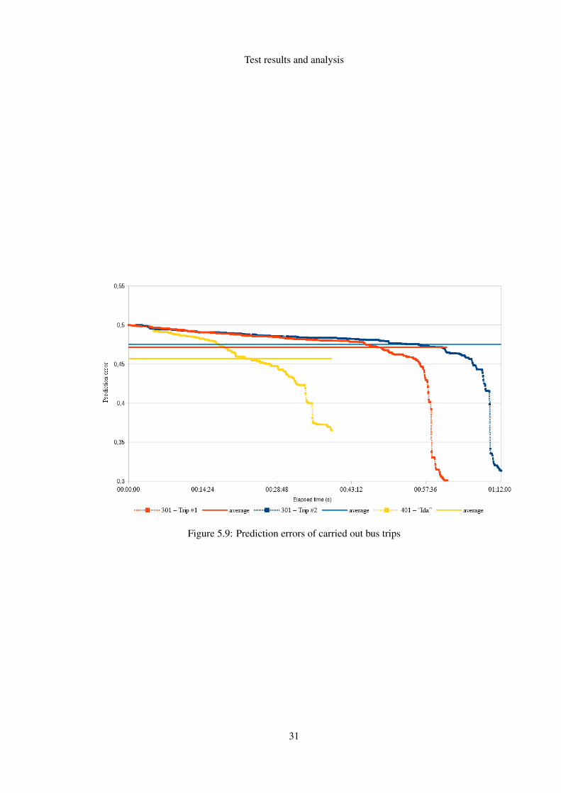
As observed in the Figure 5.9, the prediction error rises when the time prediction tends to 0,

that is, when the bus trip nears its end. By saving locally the average prediction error from the

last bus trip, the prediction error will tend to decrease when the route starts and then increase as

the TTP decreases. This behaviour is expectable the way prediction errors are updated, as it was

described in chapter 4 of this dissertation.

27


Figure 5.3: Estimation errors for the first trip of route 301

Figure 5.4: Comparison of arrival times for the first trip of route 301

28


Figure 5.5: Estimation errors for the second trip of route 301

Figure 5.6: Comparison of arrival times for the second trip of route 301

29


Figure 5.7: Estimation errors of route 401

Figure 5.8: Comparison of arrival times of route 401

30


Figure 5.9: Prediction errors of carried out bus trips

31


32

Chapter 6

Conclusion and Future Work

Conclusion

Nowadays the AVL systems used on the market are too expensive so that small and medium

companies can easily acquire these equipments. These systems have several functionalities that

are useful to the bus driver, whether they are tracking, farebox, travel time prediction or others.

While some features are relatively easy to implement, the most challenging in terms of com-

plexity is the TTP calculation. According to the literature review, we could observe that the use of

Kalman filters is highly recommended and currently used in the calculation of TTP in real time.

Through the data recorded, the SAE Light Controller proved that an Android device is able to

calculate the TTP, in real time, using the algorithm developed through the use of Kalman filters.

Although some results fail to confirm this success, we will present some possible future work so

that the accuracy of the algorithm increases to something competitive with the actual AVL systems

used on the market.

SAE Light Controller also proved to be able to overcome the two biggest challenges that it

had besides the calculation of the TTP: the Internet connection and the use of the battery. The

application only requires Internet connection to launch Maps Activity with the necessary informa-

tion to the algorithm, to record in the database all the readings made for the tracking of position,

time, start and end of route. Regarding the use of the battery of the device, it has an expected

consumption, and is perfectly controllable through the use of a cigarette lighter charger.

In conclusion, an Android device can be used as a way to compete with current AVL systems,

thus reducing the cost of acquiring the equipment in a very considerable amount, and there are

still other possible variables to be added, such as future work, to increase the accuracy of the TTP

calculation or the addition of more functionalities, in order to completely emulate a current AVL

system.

33

Conclusion and Future Work

Future Work

SAE Light Controller is capable of competing with current AVL systems on the market in

calculating the travel time prediction, one of the most challenging aspects of these systems. How-

ever, it would be interesting to minimize positioning errors by assuming that the bus is always in

the nearest point of the route’s polyline and, therefore, minimize the current travelled distance,

ending in a better travel time prediction calculated with the algorithm. To achieve this, the public

transportation’s company must be able to define a polyline for each route comprised of a set of

location points.

For an even better calculation of the TTP, instead of only working with the start and ending

times for defining the trip’s estimated time, define a trip as a set of smaller trips with start and

ending times between each stop. Therefore, the application will be able to calculate the TTP

between each and every stop in the bus route. This way, the time prediction of bus’ arrival is even

more accurate.

Google Maps has also a traffic control API and, with this, once the driver starts the bus trip,

he/she would have a prediction already taking into account possible traffic delays between bus

stops. This way, the calculated prediction would not only be influenced by real-time conditions,

but also start taking account the route’s traffic conditions.

The use of more different sensors, such as the accelerometer of the device among other pos-

sible, increases the complexity of the algorithm and, consequently, increases the precision of the

data, minimizing the accumulated error.

In the testing phase, it may be interesting to try out different data reading frequencies. In this

way it is possible to verify if the increase or reduction of this frequency causes more precise results

and what is its impact in the time of processing and use of the battery.

Finally, by storing the bus’ location in the database, SAE Light Controller is able to achieve

many interesting features, currently associated with fully developed AVL systems, such as:

• Bus tracking: By sending the stored coordinates to every application, the bus’ driver will

be able to plan if he wants to stop and increase the delay in an already behind the schedule

trip or let the customers on the bus’ stop to wait for the next bus. The companies will also

be able to track the bus to be able to better plan its schedule efficiency, better respond to an

emergency, etc.

• Customer assistance: Let the customers know, in real-time, the current time needed for the

bus to arrive, through the use of several methods, such as dynamic message signs;

• Manager of headsign and farebox;

• Onboard automatic passenger counting: let the companies to record the number of passen-

gers boarding.

34

References

[FHMS03] Peter Gregory Furth, Brendon J Hemily, T Muller, and James G Strathman.Uses of archived AVL-APC data to improve transit performance and manage-ment: Review and potential. Transportation Research Board Washington, DC,USA, 2003.

[Kal60] Rudolph Emil Kalman. A new approach to linear filtering and prediction prob-lems. Journal of Fluids Engineering, 82(1):35–45, 1960.

[LZ99] Wei-Hua Lin and Jian Zeng. Experimental study of real-time bus arrival timeprediction with gps data. Transportation Research Record: Journal of theTransportation Research Board, (1666):101–109, 1999.

[May82] Peter S Maybeck. Stochastic models, estimation, and control, volume 3. Aca-demic press, 1982.

[MBP+04] George Mintsis, Socrates Basbas, Panos Papaioannou, Christos Taxiltaris, andIN Tziavos. Applications of gps technology in the land transportation system.European journal of operational Research, 152(2):399–409, 2004.

[MMMMdSG15] Luis Moreira-Matias, Joao Mendes-Moreira, Jorge Freire de Sousa, and JoaoGama. Improving mass transit operations by using avl-based systems: A sur-vey. IEEE Transactions on Intelligent Transportation Systems, 2015.

[Mon07] Torin Monahan. “war rooms” of the street: Surveillance practices in transporta-tion control centers. The Communication Review, 10(4):367–389, 2007.

[OPM12] Thomas Olutoyin Oshin, Stefan Poslad, and Andy Ma. Improving the energy-efficiency of gps based location sensing smartphone applications. In Trust,Security and Privacy in Computing and Communications (TrustCom), 2012IEEE 11th International Conference on, pages 1698–1705. IEEE, 2012.

[Par08] Doug J Parker. AVL systems for bus transit: Update. Number 73. TransportationResearch Board, 2008.

[PRM+10] Bratislav Predic, Dejan Rancic, Aleksandar Milosavljevic, et al. Impacts of ap-plying automated vehicle location systems to public bus transport management.Journal of Research and Practice in Information Technology, 42(2):79, 2010.

[TYK05] Adam Theiss, David C Yen, and Cheng-Yuan Ku. Global positioning systems:an analysis of applications, current development and future implementations.Computer Standards & Interfaces, 27(2):89–100, 2005.

35

Documents

SAE Light Controller – Automatic vehicle location using