SADDLE POINT OF ATTACHMENT

IN HORSESHOE VORTEX SYSTEM

_______________________________________

A Thesis presented to the Faculty of the Graduate School

at the University of Missouri-Columbia

_______________________________________________________

In Partial Fulfillment

of the Requirements for the Degree

Master of Science

_____________________________________________________

by

CHENXING ZHANG

Dr. Chung-Lung Chen, Thesis Supervisor

JULY 2015

  

The undersigned, appointed by the dean of the Graduate School, have examined the thesis entitled

SADDLE POINT OF ATTACHMENT IN HORSESHOE

VORTEX SYSTEM

Presented by Chenxing Zhang,

A candidate for the degree of Master of Science

And hereby certify that, in their opinion, it is worthy of acceptance.

Professor Chung-Lung Chen

Professor Gary Solbrekken

Professor Carmen Chicone

ii  

ACKNOWLEDGEMENTS

I would like to express the deepest appreciation to my advisor, Dr. CHEN. He

continually supports me and has shown dedication and keen interest in me at every stage

of my research. His inspirations, timely suggestions given with kindness, enthusiasm and

dynamism have enabled me to complete my thesis. His idea always is refresh and

enlighten me, which helps me to think more and dig more.

I owe a deep sense of gratitude to Sean and Simon for their continuing guidance, and

friendly suggestions during the project work. I am sincerely grateful to them for sharing

their truthful and illuminating views on a number of issues related to the project. They are

the experts for solving problems.

I’m grateful to my friends Chen Bo, Jingwen, Tiancheng who helped me a lot during

the whole project.

Finally, I would like to thank my parents. They help to financially support to me

during the entire project, and they encourage me not to give it up, and let me keep on

working with the project.

 

 

 

iii  

 

TABLE OF CONTENTS

ACKNOWLEDGEMENTS ............................................................................................................ II 

TABLE OF CONTENTS .............................................................................................................. III 

LIST OF ILLUSTRATIONS ......................................................................................................... V 

NOMENCLATURE .................................................................................................................... VII 

ABSTRACT ................................................................................................................................... X 

CHAPTER 1 INTRODUCTION ................................................................................................. 1 

1.1  Background ...................................................................................................................... 1 

1.2  Previous work ................................................................................................................... 2 

1.2.1  Horseshoe vortex ...................................................................................................... 2 

1.2.2  Saddle point of attachment ........................................................................................ 2 

1.2.3  Jet in crossflow ......................................................................................................... 6 

1.3  Present work ..................................................................................................................... 9 

CHAPTER 2  MATHEMETICAL ANALYSIS ........................................................................ 10 

2.1 Critical point in the flow patterns .................................................................................... 10 

2.2 Solving Equation ............................................................................................................. 11 

CHAPTER 3  NUMERICAL MODELING ............................................................................... 15 

3.1  Geometry and boundary conditions ............................................................................... 15 

3.1.1  Laminar juncture flow ............................................................................................. 15 

3.1.2  Jet in crossflow ....................................................................................................... 17 

iv  

3.2  Simulation approach ....................................................................................................... 19 

3.3 Grid independent study ................................................................................................... 20 

CHAPTER 4  RESULTS AND DISCUSSION ......................................................................... 23 

4.1  Validation with juncture flow ........................................................................................ 23 

4.2  Jet in crossflow with different velocity ratios ................................................................ 25 

4.2.1  Results for d=20D ................................................................................................... 25 

4.2.2  Results for d=1.6D .................................................................................................. 30 

4.3 Topology rules .................................................................................................................. 31 

4.4 Effect of boundary layer thickness .................................................................................. 31 

4.5 Effects of oscillation ........................................................................................................ 33 

CHAPTER 5  CONCLUSION ................................................................................................... 37 

REFERENCES ............................................................................................................................. 38 

 

 

v  

LIST OF ILLUSTRATIONS

Figure 1. Saddle point of separation in front of cylinder (Ref. [11],[19]) ....................................... 3 

Figure 2. Saddle point of attachment in simulation (Ref. [22, 23]) ................................................. 4 

Figure 3. Laser light sheet visualization (Ref. [24]) ........................................................................ 4 

Figure 4. Impact of aspect ratio with boundary layer thickness (Ref. [27]) .................................... 5 

Figure 5. Jet in crossflow ................................................................................................................. 6 

Figure 6. Sketch of jet interactions from symmetry plane (Ref. [35]) ............................................. 7 

Figure 7. Jet in crossflow side-view in the plate of symmetry (Ref. [34])....................................... 8 

Figure 8. X, U and Vorticity in xyz direction (Ref. [43]) .............................................................. 11 

Figure 9. a) Saddle point ( / ) b) Degenerate form ( / ) c) Node ( / )13 

Figure 10. Flow upstream of a cylinder standing on a flat plate .................................................... 15 

Figure 11. Blasius Solution ............................................................................................................ 16 

Figure 12. Velocity profile at the flow inlet ................................................................................... 16 

Figure 13. Numerical model of the jet in crossflow (From side and top views) ............................ 17 

Figure 14. Velocity profile for R=2.5, 2, 1.5 ................................................................................. 19 

Figure 15. Mesh details for different grid ...................................................................................... 21 

Figure 16. Comparison results from Grids A, B and C .................................................................. 22 

Figure 17. Juncture flow from a) Symmetry plane side view. b) From top view. ......................... 24 

Figure 18. For R=2.5 jet in crossflow ............................................................................................ 26 

Figure 19. 3D view for jet in crossflow ......................................................................................... 27 

Figure 20. Streamlines at the symmetry plane for R=2 ................................................................. 28 

Figure 21. Top view with limiting streamlines for R=2 ................................................................ 28 

Figure 22. Streamlines at the symmetry plane ............................................................................... 29 

Figure 23. Streamlines at the symmetry plane d=1.6D with a) R=1.5 and b) R=2.5 ..................... 30 

vi  

Figure 24. Effect of various distance on horseshoe vortex (a) d=1D (saddle point of separation) (b)

d=1.6D (degenerate form) (c) d=20D (saddle point of attachment) ...................................... 32 

Figure 25. Velocity varying with time (T= 0.68τ and T= 2.72τ) ................................................... 34 

Figure 26. Instaneous streamlines under T= 0.68τ (t=0.05T and t=0.5T); .................................... 35 

Figure 27. Instaneous streamlines with T= 2.72τ (t=0.05T and t=0.5T); ...................................... 35 

Figure 28. The location of the singular point(x/D) and distance between the singular point and the

upstream edge of the jet ( ) varying with period time (T= 0.68τ and T= 2.72τ) ................. 36 

   

vii  

NOMENCLATURE

Velocity in x direction (m/s)

v Velocity in y direction (m/s)

w Velocity in z direction (m/s)

U Velocity vector (m/s)

H Cylinder height (m)

D Diameter of cylinder or jet (m)

Dynamic viscosity (Ns/ )

Density (kg/ )

p Pressure (kg / )

Kinematic viscosity (m/s2)

Kinematic pressure ( / )

d Distance between inlet and center of jet (m)

Distance between the singular point and the upstream edge of the cylinder (m)

Distance between the singular point and the upstream edge of the jet (m)

Average velocity of jet (m/s)

Velocity of crossflow (m/s)

Amplitudeofthejetflow(m/s)

TPeriodofthevelocityfunction s

Velocityofthejetflowsteadystate(m/s)

t Time (s)

τ Characteristic time length (D/ )

viii  

Jacobian Matrix

Vorticity vector

Velocity Ratio / )

Velocity ratio of steady state ( / )

′ Velocity ratio of amplitude ( ′ / )

Reynolds number ( / )

Reynolds number of jet ( / )

x/D Location of singular point

λ Eigenvalue of equations

m Eigenvector slope

Angle of separation or attachment

V Shear layer vortex

S Saddle point

N Node

S’ Half saddle point

N’ Half node

Boundary layer thickness (m)

Boundary layer thickness at the upstream edge of the jet (m)

ζ Vorticity in x direction ( )

η Vorticity in y direction ( )

ξ Vorticity in z direction ( )

Abbreviations

AFRL Air Force Research Laboratory

ix  

PIV Particle Image Velocimetry

SIMPLE Semi-Implicit Method for Pressure-Linked Equations

x  

SADDLE POINT OF ATTACHMENT IN HORSESHOE VORTEX SYSTEM

Chenxing Zhang

Dr. Chung-Lung Chen, Thesis Advisor

ABSTRACT

Laminar juncture flow has been well studied experimentally and numerically in recent

years. New topology upstream in terms of saddle point of attachment has been investigated by

both approaches. In this work, the obstacle standing on the flat plate was replaced with a jet flow.

Numerical simulation and theoretical analysis were performed to investigate the upstream

topology. The numerical results were validated with the mathematical theory and topology rules.

The upstream critical point satisfies the condition of occurrence for saddle point of attachment in

the horseshoe vortex system. In addition to the classical topology led by the saddle point of

separation, the new topology led by saddle point of attachment was found for the first time in a

crossflow with jet. The transition of the critical point from separation to attachment is

determined by the ratio of the velocity of the jet to the velocity of the crossflow, the boundary

layer thickness of the flat plate, and the oscillation of the jet. When the boundary layer thickness

at the upstream edge of the jet is close to one diameter, the flow topology is led by a saddle point

of attachment. Variation of the velocity ratio has no effect on the topology, but changes the

location of the saddle point. When the boundary layer thickness is about 0.2 diameter, decreasing

the velocity ratio will change the flow topology from the attachment form to the degenerate form.

The transition of the critical point from separation to attachment was also observed when the

boundary layer thickness increased while the velocity ratio remained constant. Furthermore, it

was observed that, under a high frequency oscillation of a jet, the characteristics of the critical

point could change between separation and attachment.

1  

Chapter 1 INTRODUCTION

1.1 Background

           Flow past an obstacle sitting on a flat plate is a fundamental fluid dynamics

problem. This basic juncture flow represents a class of realistic flows encountered in our

daily lives such as flow pass buildings, cooling towers, chimney, river bridge pillar flow

and the secondary flow in turbines, wing-fuselage junctures, wing-pylon junctures, and

multibody junctures of launching space shuttle. It is commonly conceived that when a

boundary layer encounters a bluff body protuberance, the flow separates and rolls up to

form a horseshoe vortex or a system of horseshoe vortices. This three dimensional

horseshoe vortex flow influence total pressure losses. Therefore, to understand the near

field flow with attachment or separation can become very important. In the formation of

the horseshoe vortex, high-pressure stagnation point forms on the windward side of the

obstacle, and this creates an adverse pressure gradient for the flow approaching the

obstacle. The adverse pressure gradient causes the boundary layer of the flow across the

ground to detach and roll up into a vortex. The horseshoe vortex system usually exists not

only in the juncture flow but also in jet crossflow interaction. The singular points always

occur with the vortex system. Therefore, the characteristics of these singular points near

the wall will be investigated both in juncture flow and jet in a crossflow.

2  

1.2 Previous work

1.2.1 Horseshoe vortex

For a laminar juncture flow, the horseshoe vortex system upstream cylinder has

been found both in simulations [1-3] and experimental studies [4-6]. The existence of

horseshoe vortex in juncture flow was proven by Schwind[4] and Baker[7] earlier, and

smoke flow visualization was used to complete the measurements. Furthermore the

formation of horseshoe vortex in a three-dimensional computational way has been

investigated by Eckerle[8]. The relationship between the Reynolds number and the

number of horseshoe vortex was discovered by Thompson[9]. In addition to steady

system, unsteady horseshoe vortex systems has been done using numerical method by

Visbal[10]. Different Re in range of 500-5400 have been individually tested to find the

separation and attachment line. In Agui[11]’s investigation, results from measurements

and flow visualization have confirmed that the horseshoe vortex showed a low shear

region associated with separation. Sabatino and Smith[12, 13] both gave an investigation

for the connection between turbulent boundary layer and unsteady horseshoe vortex

system. They also performed several experiments to show that the symmetry plane is

characterized by a stable-focus streamline topology.

1.2.2 Saddle point of attachment

During the numerical simulation, the theory of topology is frequently used to gain

physical meaningful insight into this kind of flow. Because of its complex nature in a

three-dimensional situation, researchers usually use streamlines at the symmetry plane

3  

and limiting streamlines (oil flow pattern) at wall surface to help understand the

phenomena in the analysis of the numerical results. These streamline patterns are featured

by topological singular points of which the streamline slope is indeterminate. The critical

points can be classified as saddle points, nodes, foci or spiral points [14-18]. Moreover

normal to the wall, the flow repels away from a critical point referred to as ‘separation’.

On the other hand, if the flow moves toward a critical point, we call it ‘attachment’.

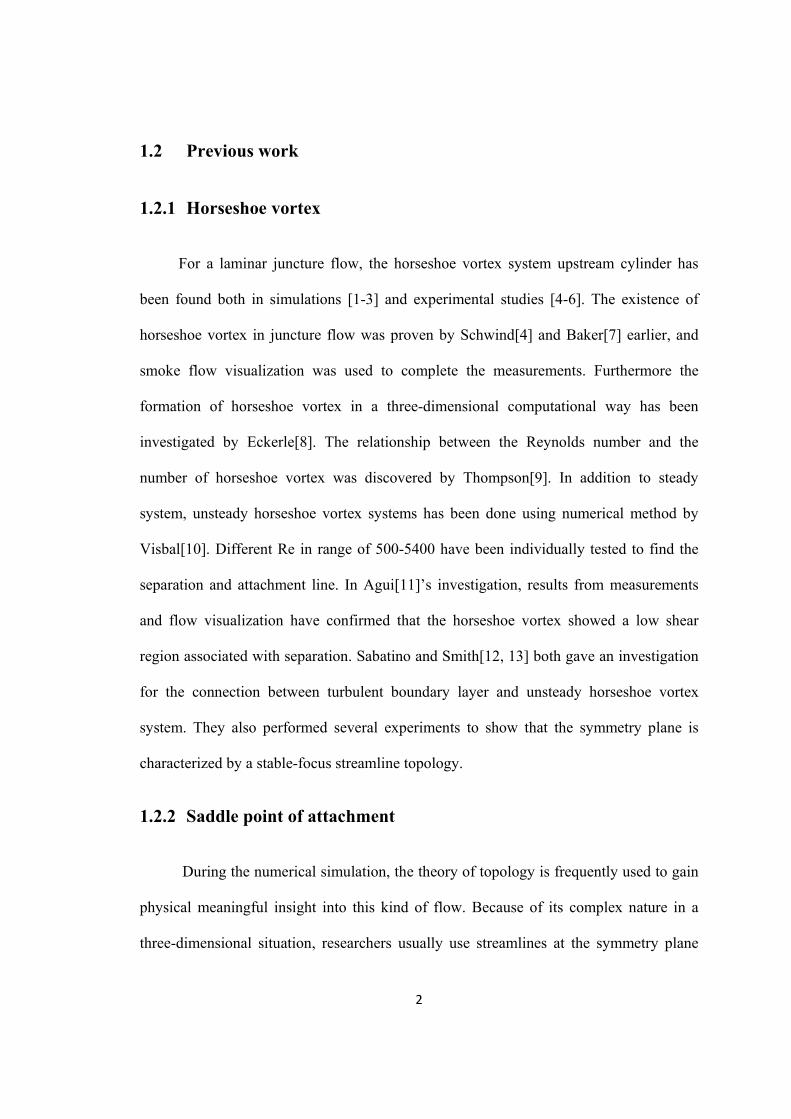
For the laminar juncture flow, a saddle point of separation existing in the upstream

cylinder has been postulated by several research groups [10, 11, 13] shown in Fig.1.

Figure 1. Saddle point of separation in front of cylinder (Ref. [11],[19])

Since then, it has been continually treated as a saddle of separation until Visbal[20],

Hung and Chen[21, 22] demonstrated a new topology. This new flow topology shares the

same top view with the traditional one. From the top view, the singular point is a full

saddle point, while from the side view, it is a half node to which the flow moves.

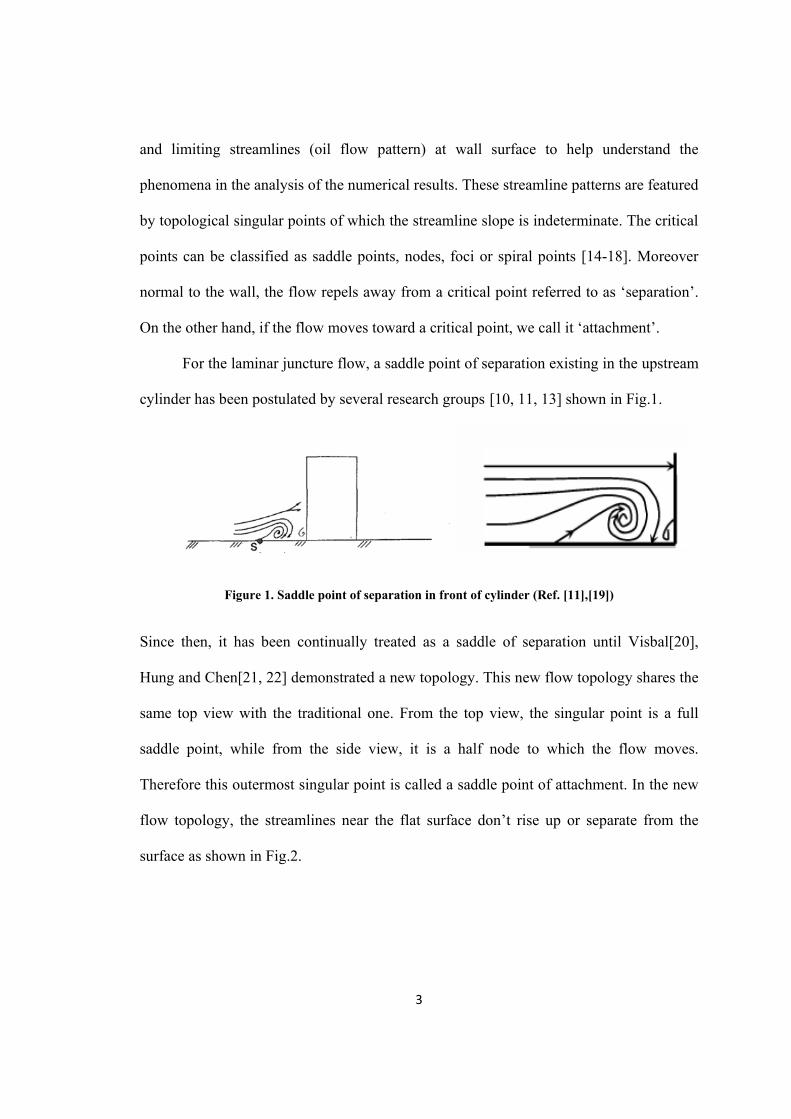
Therefore this outermost singular point is called a saddle point of attachment. In the new

flow topology, the streamlines near the flat surface don’t rise up or separate from the

surface as shown in Fig.2.

4  

 

Figure 2. Saddle point of attachment in simulation (Ref. [22, 23])

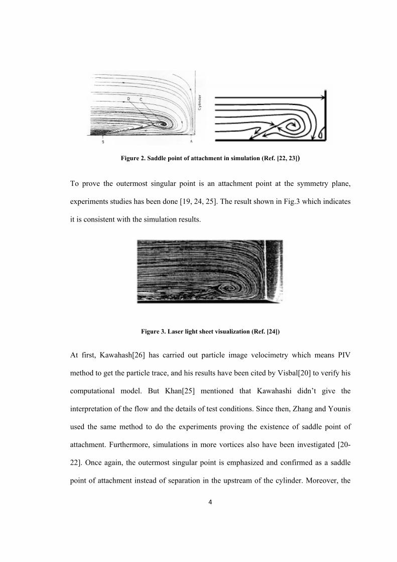
To prove the outermost singular point is an attachment point at the symmetry plane,

experiments studies has been done [19, 24, 25]. The result shown in Fig.3 which indicates

it is consistent with the simulation results.

Figure 3. Laser light sheet visualization (Ref. [24])

At first, Kawahash[26] has carried out particle image velocimetry which means PIV

method to get the particle trace, and his results have been cited by Visbal[20] to verify his

computational model. But Khan[25] mentioned that Kawahashi didn’t give the

interpretation of the flow and the details of test conditions. Since then, Zhang and Younis

used the same method to do the experiments proving the existence of saddle point of

attachment. Furthermore, simulations in more vortices also have been investigated [20-

22]. Once again, the outermost singular point is emphasized and confirmed as a saddle

point of attachment instead of separation in the upstream of the cylinder. Moreover, the

5  

Mach number related to the juncture flow in various Reynolds numbers is investigated by

Chen[21].

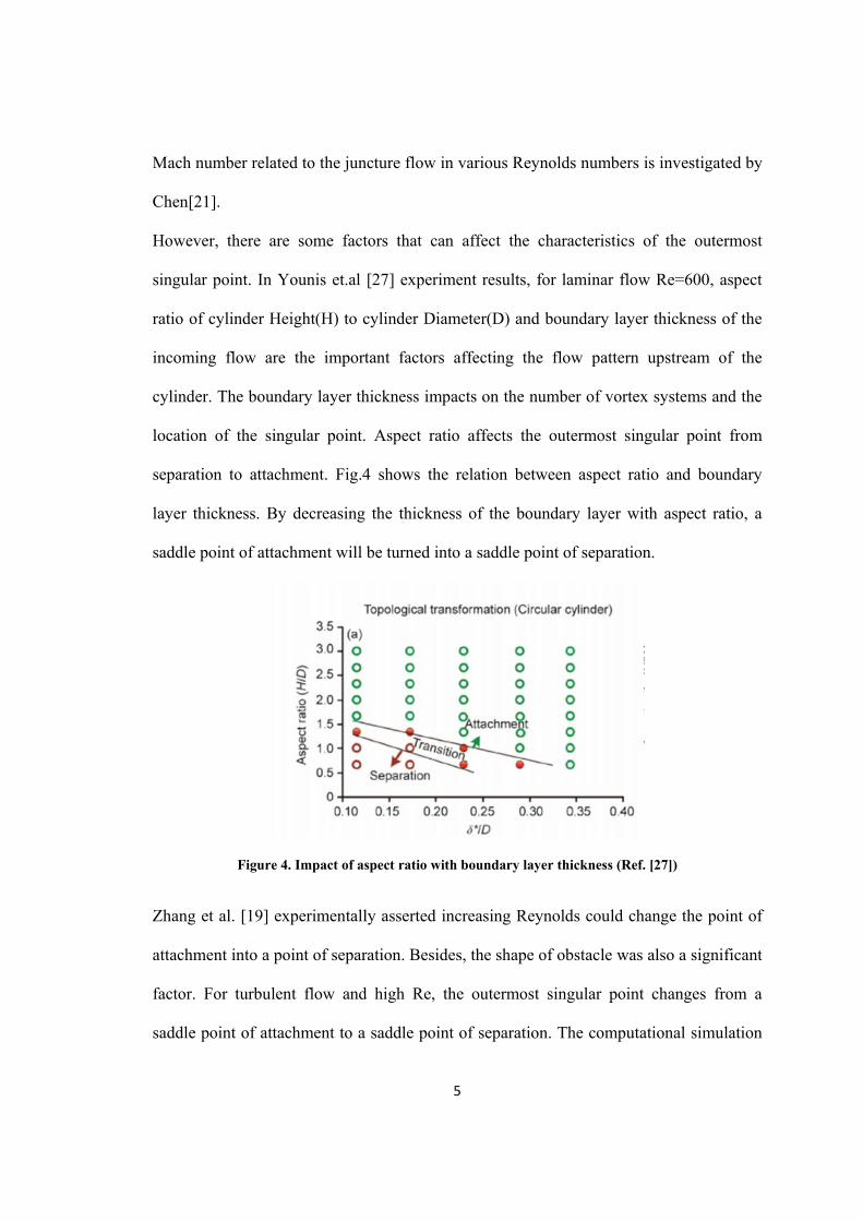
However, there are some factors that can affect the characteristics of the outermost

singular point. In Younis et.al [27] experiment results, for laminar flow Re=600, aspect

ratio of cylinder Height(H) to cylinder Diameter(D) and boundary layer thickness of the

incoming flow are the important factors affecting the flow pattern upstream of the

cylinder. The boundary layer thickness impacts on the number of vortex systems and the

location of the singular point. Aspect ratio affects the outermost singular point from

separation to attachment. Fig.4 shows the relation between aspect ratio and boundary

layer thickness. By decreasing the thickness of the boundary layer with aspect ratio, a

saddle point of attachment will be turned into a saddle point of separation.

Figure 4. Impact of aspect ratio with boundary layer thickness (Ref. [27])

Zhang et al. [19] experimentally asserted increasing Reynolds could change the point of

attachment into a point of separation. Besides, the shape of obstacle was also a significant

factor. For turbulent flow and high Re, the outermost singular point changes from a

saddle point of attachment to a saddle point of separation. The computational simulation

6  

of turbulent flow has been studied by Hung and Chen [21, 22] for checking the property

of the outermost singular point. Their results were agreed with the experimental studies

(Sedney&Kitchens) which showed the character of the upstream the outermost singular

point is a saddle point of separation in a turbulent flow. Thus, the saddle point of

attachment only existed with low-Re laminar, but not high-Re turbulent horseshoe vortex

system; this theory has been mentioned by Chen[28]. The existence of saddle point of

separation in the turbulent model also has been investigated by Khan[25]. In his research,

the outermost singular point is always a saddle point of separation when the Reynolds

number is from 1900-6500.

1.2.3 Jet in crossflow

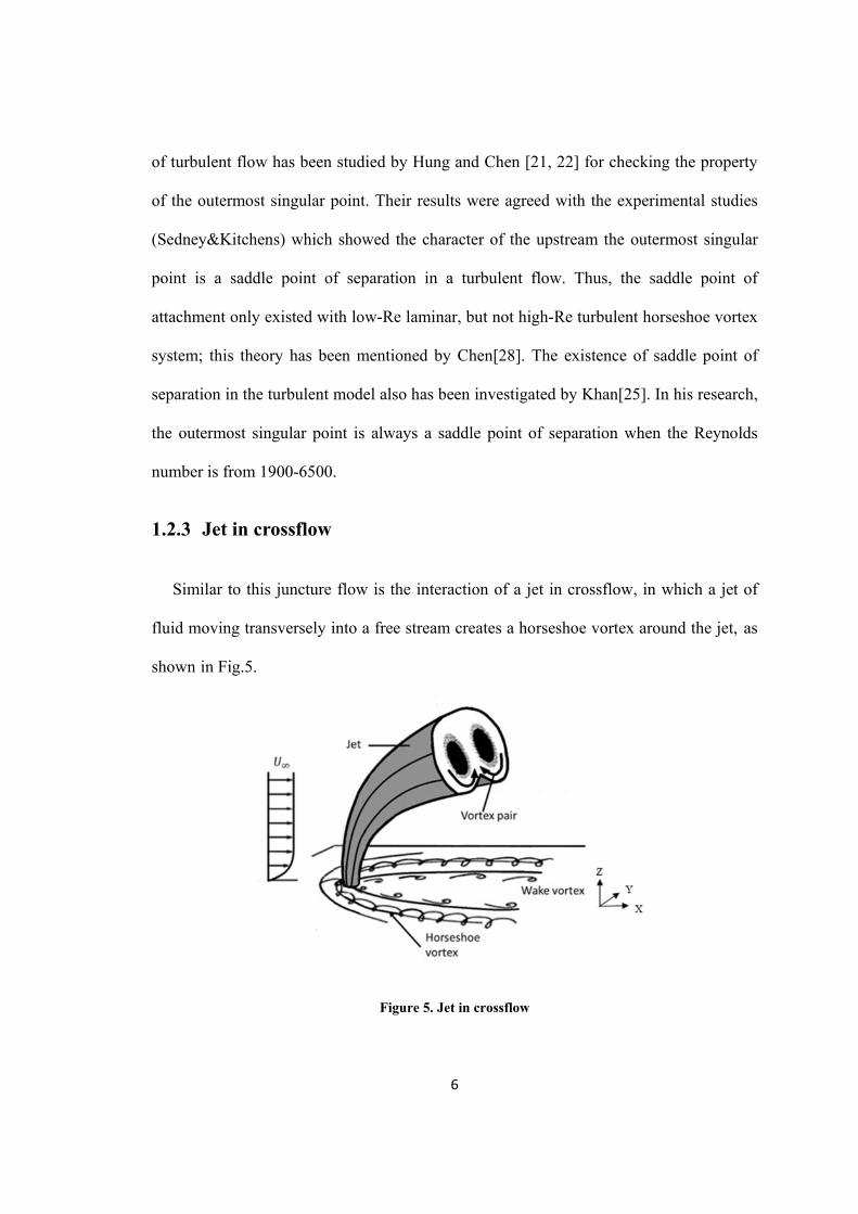
Similar to this juncture flow is the interaction of a jet in crossflow, in which a jet of

fluid moving transversely into a free stream creates a horseshoe vortex around the jet, as

shown in Fig.5.

Figure 5. Jet in crossflow

7  

Discharge of effluent into rivers and oceans, mixing section of gas turbine engines, film

cooling, injection and flow control are a few of the important applications of this flow.

Usually jet fluid blows out of a round pipe and mixes with the crossflow fluid travelling

in x direction [29-31]. An experiment about low velocity ratio around a circular jet in

crossflow has been done by Cambonie[32], using volumetric velocimetry measurements

to discuss the velocity fields. Some other researches [33, 34] also noticed that there is a

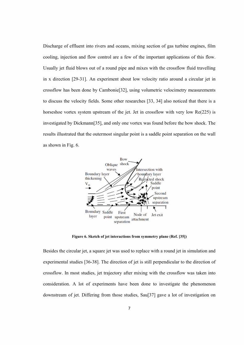
horseshoe vortex system upstream of the jet. Jet in crossflow with very low Re(225) is

investigated by Dickmann[35], and only one vortex was found before the bow shock. The

results illustrated that the outermost singular point is a saddle point separation on the wall

as shown in Fig. 6.

Figure 6. Sketch of jet interactions from symmetry plane (Ref. [35])

Besides the circular jet, a square jet was used to replace with a round jet in simulation and

experimental studies [36-38]. The direction of jet is still perpendicular to the direction of

crossflow. In most studies, jet trajectory after mixing with the crossflow was taken into

consideration. A lot of experiments have been done to investigate the phenomenon

downstream of jet. Differing from those studies, Sau[37] gave a lot of investigation on

8  

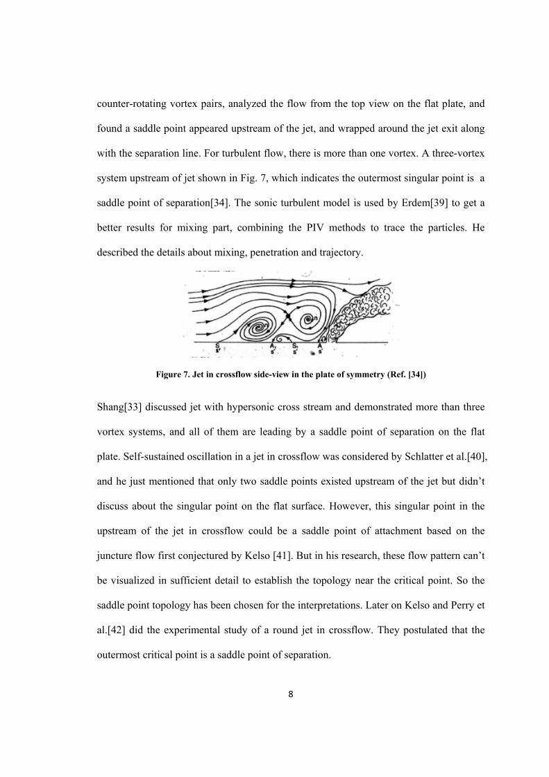
counter-rotating vortex pairs, analyzed the flow from the top view on the flat plate, and

found a saddle point appeared upstream of the jet, and wrapped around the jet exit along

with the separation line. For turbulent flow, there is more than one vortex. A three-vortex

system upstream of jet shown in Fig. 7, which indicates the outermost singular point is a

saddle point of separation[34]. The sonic turbulent model is used by Erdem[39] to get a

better results for mixing part, combining the PIV methods to trace the particles. He

described the details about mixing, penetration and trajectory.

Figure 7. Jet in crossflow side-view in the plate of symmetry (Ref. [34])

Shang[33] discussed jet with hypersonic cross stream and demonstrated more than three

vortex systems, and all of them are leading by a saddle point of separation on the flat

plate. Self-sustained oscillation in a jet in crossflow was considered by Schlatter et al.[40],

and he just mentioned that only two saddle points existed upstream of the jet but didn’t

discuss about the singular point on the flat surface. However, this singular point in the

upstream of the jet in crossflow could be a saddle point of attachment based on the

juncture flow first conjectured by Kelso [41]. But in his research, these flow pattern can’t

be visualized in sufficient detail to establish the topology near the critical point. So the

saddle point topology has been chosen for the interpretations. Later on Kelso and Perry et

al.[42] did the experimental study of a round jet in crossflow. They postulated that the

outermost critical point is a saddle point of separation.

9  

1.3 Present work

In this work, numerical simulation was carried out to investigate the upstream flow

topology both in the juncture flow and jet in crossflow. Combining with mathematical

analysis, the existence of the saddle point of attachment in a horseshoe vortex system was

demonstrated under certain conditions. The upstream topologies and the location of the

saddle point were studied at various velocity profiles of the jet. In addition, the effects of

boundary layer thickness and the unsteady jet were investigated to examine the

characteristics of the outermost singular point.

10  

Chapter 2 MATHEMETICAL ANALYSIS

2.1 Critical point in the flow patterns

The characteristics of critical point are related to different variable parameters like

velocity, vorticity and pressure. Analysis of the critical point is generally used to

understand flow patterns. When considering the flow of a viscous fluid over a surface, it

is assumed that the velocity components are Taylor series expandable about the critical

point in three-dimensional system, then it can be written in Eq. 1

∅ 1

where ∅ is a scalar function of real physical space X. F is a 3 x 3 Jacobian matrix of

the dynamic system at the critical point. U is the velocity vector. Put the equation in a

phase space form, then

’ 2

Which means

3

For viscous flow, the non-slip condition requires that U=0 at the wall surface z=0. So

velocity U is represented in x, y and z directions shown Eq.4

4

11  

2.2 Solving Equation

For incompressible flow, the continuity equation is

0 5

Substituting Eq.4 into Eq.5,

2 0 6

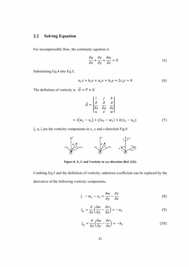
The definition of vorticity is

7

ξ, η, ζ are the vorticity components in x, y and z direction Fig.8

Figure 8. X, U and Vorticity in xyz direction (Ref. [43])

Combing Eq.5 and the definition of vorticity, unknown coefficient can be replaced by the

derivative of the following vorticity components.

ξ = 8

ξ 9

ξ 10

12  

η 11

η 12

η 13

ζ 14

Due to the definition of vorticity, and can’t be zero. For different value x, y and z,

Eq.6 must keep zero, therefore and have to be zero. Then,

12

12

η ξ 15

Combine the Navier Stokes equation with Eq.4, the relations with pressure (p) and and

can be obtained.

∙ 2 0 16

∙ 2 0 17

Both sides divided by

∙ 2 0 18

2 19

2 20

where P is kinematic pressure and is kinematic viscousity. Finally, the Jacobian Matrix

F is

13  

η η2

-ξ -ξ2

0 012

ξ η

Then Eq.4 is

/2

/2

12

21

Consider the case of a flow with a plane of symmetry in the xz plane, so that

0. Therefore at the plane y=0, Eq. 21 can be written as

∙ 2

012

22

so the eigenvalues of the matrix A in the Eq. 22 are

12

, 23

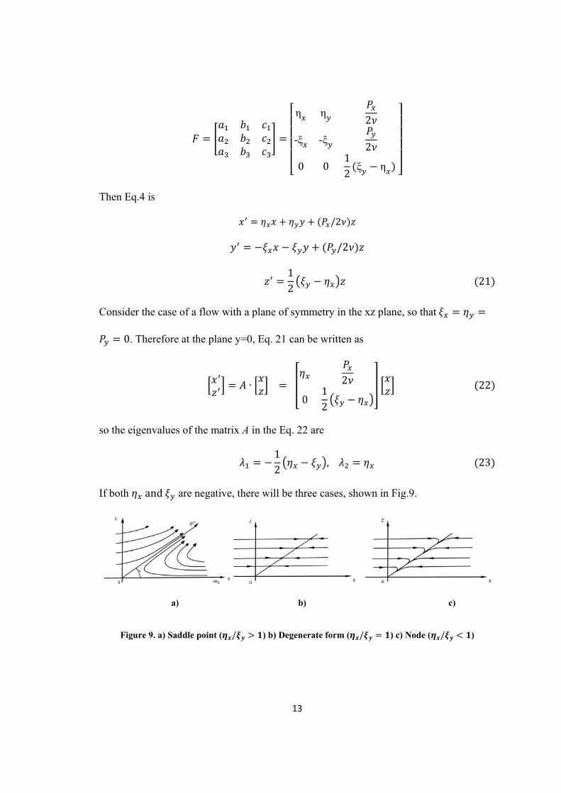
If both and are negative, there will be three cases, shown in Fig.9.

a) b) c)

Figure 9. a) Saddle point ( / ) b) Degenerate form ( / ) c) Node ( / )

14  

When (a) / 1, there is one positive and one negative eigenvalue, so the singular

point will be a saddle point. When (b) / 1, there is a zero eigenvalue, so the

singular point will be a degenerate form. When (c) / 1, there are two negative real

eigenvalues, so the singular point will be a stable node.

From the results, it is clear that vorticity components and pressure are the significant

factors determining the formation of the node and the saddle point. The eigenvector

slopes (m) of the matrix A are

2 12

32 η 24

0

This implies that flow separates or attaches from/to the wall with an angle .

3η 25

15  

Chapter 3 NUMERICAL MODELING

In this chapter, geometry and boundary conditions are described for the juncture flow and

jet in crossflow. Then numerical approach is briefly introduced followed by grid

independent study.

3.1 Geometry and boundary conditions

3.1.1 Laminar juncture flow

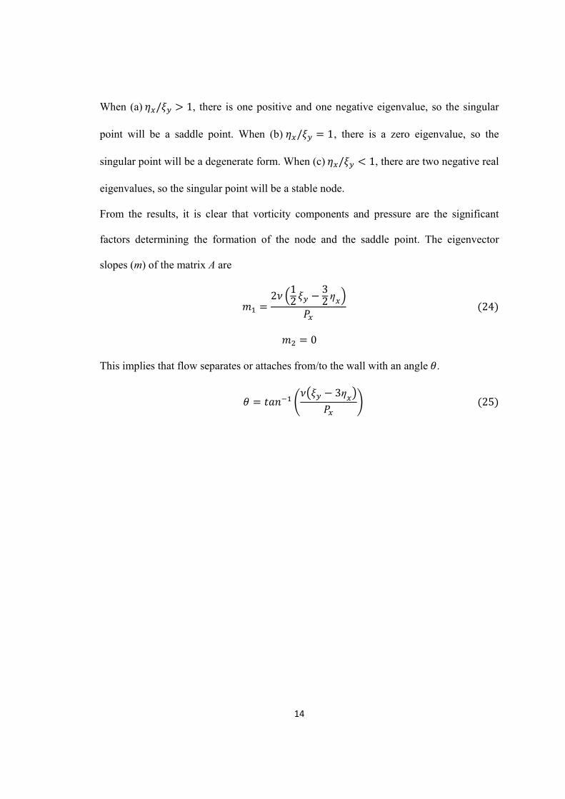
In order to ensure appropriate grid distribution and the accuracy of modeling,

laminar juncture flow has been done before the simulation for jet in crossflow. The

boundary condition for the incoming crossflow and the computational domain are the

same as those et al. [21, 22] shown in Fig.10.

Figure 10. Flow upstream of a cylinder standing on a flat plate (Ref. [22])

Computational domain is 50D×4D×5D. D is the diameter of the cylinder, which is

derived from the crossflow Re=500 and Mach number is 0.2. The origin of coordinates is

at the center of the cylinder. An incoming boundary layer of 0.1D is at initial

16  

location which is 20D away from the center of the cylinder. At y= 4D plane and the

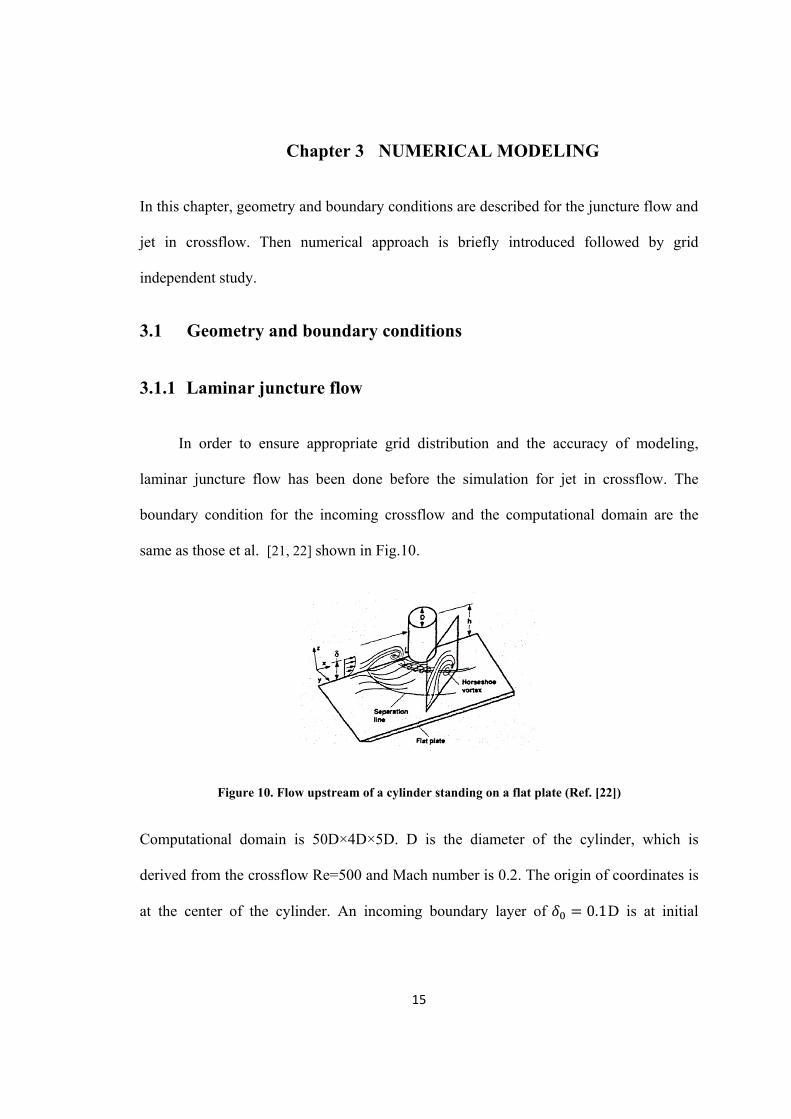
crossflow inlet plane, the boundary layer thickness will grow as

5.0 5.0 26

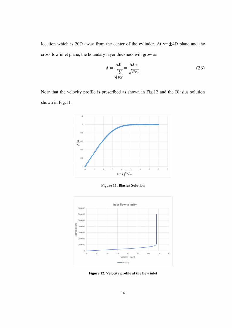
Note that the velocity profile is prescribed as shown in Fig.12 and the Blasius solution

shown in Fig.11.

Figure 11. Blasius Solution

 

Figure 12. Velocity profile at the flow inlet

17  

Symmetry conditions are applied at the top surface (z=5D plane) of computational

domain and also applied to the y=0 plane. Thus, only a half cylinder is included in the

computational domain. A no-slip wall condition is applied on the flat surface (z=0) and

cylinder wall surface. The results of juncture flow will be discussed in Chapter 4.1. 

3.1.2 Jet in crossflow

For validating the numerical model with a juncture flow, the boundary condition

for the incoming crossflow and the computational domain are the same as juncture flow.

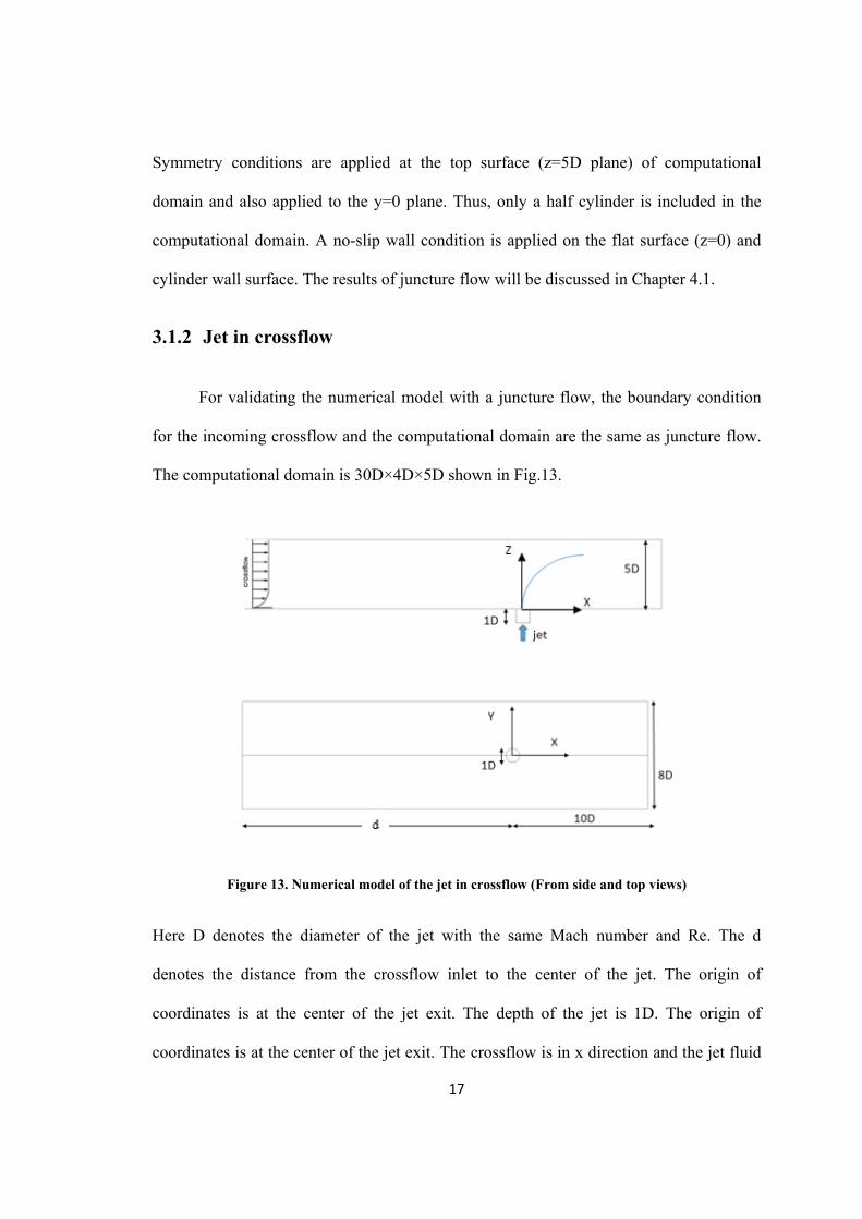
The computational domain is 30D×4D×5D shown in Fig.13.

 

Figure 13. Numerical model of the jet in crossflow (From side and top views)

Here D denotes the diameter of the jet with the same Mach number and Re. The d

denotes the distance from the crossflow inlet to the center of the jet. The origin of

coordinates is at the center of the jet exit. The depth of the jet is 1D. The origin of

coordinates is at the center of the jet exit. The crossflow is in x direction and the jet fluid

18  

is along with z direction. An incoming boundary layer of 0.1 . At y= 4D plane

and crossflow inlet plane, the boundary layer thickness will grow based on the Eq.26. As

a result, the boundary layer thickness at the upstream edge of the jet ( ) is 1.001D when

d=20D, which is the same setup as ref [20, 21, 24, 25]. To study the effects of the

boundary layer thickness, d is variable in the corresponding discussion. Symmetry and

no-slip wall conditions are applied to the same plane as those in the juncture flow.

Velocity ratio R is the average velocity of the jet over the velocity of the

crossflow. To keep the existence of a horseshoe vortex, velocity ratio can’t be too

small[32, 44]. Three different velocity ratios (R =2.5, 2 and 1.5) are discussed about the

effects on the outermost singular point. For R = 2.5, 2 and 1.5, are 1250, 1000 and

750 respectively based on the following equation,  

27

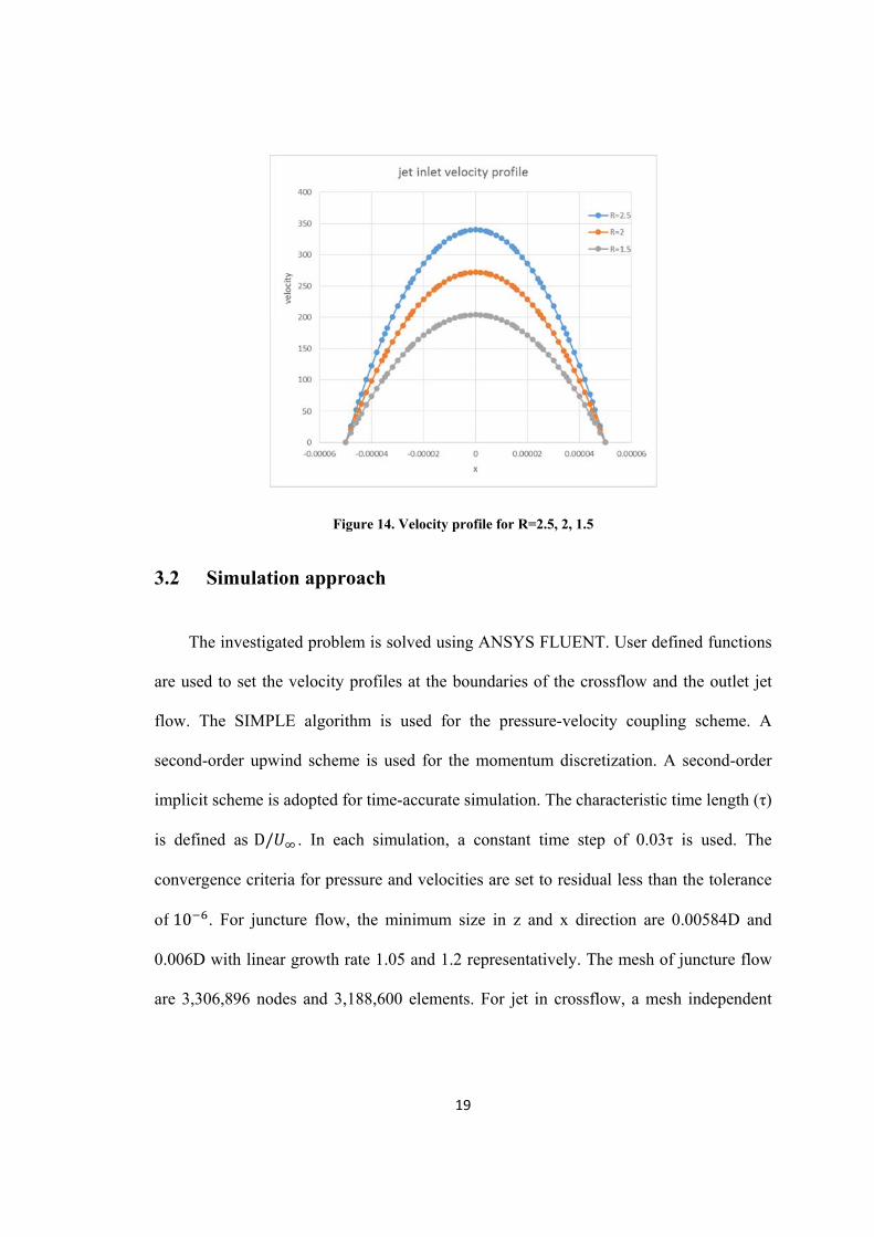
Inlet velocity profile of the jet is assumed to be a fully developed laminar flow written in

Eq.28 (Fig.14)

2 1

2

28

19  

Figure 14. Velocity profile for R=2.5, 2, 1.5

3.2 Simulation approach

The investigated problem is solved using ANSYS FLUENT. User defined functions

are used to set the velocity profiles at the boundaries of the crossflow and the outlet jet

flow. The SIMPLE algorithm is used for the pressure-velocity coupling scheme. A

second-order upwind scheme is used for the momentum discretization. A second-order

implicit scheme is adopted for time-accurate simulation. The characteristic time length (τ)

is defined as D/ . In each simulation, a constant time step of 0.03τ is used. The

convergence criteria for pressure and velocities are set to residual less than the tolerance

of10 . For juncture flow, the minimum size in z and x direction are 0.00584D and

0.006D with linear growth rate 1.05 and 1.2 representatively. The mesh of juncture flow

are 3,306,896 nodes and 3,188,600 elements. For jet in crossflow, a mesh independent

20  

study has been made and shown in Chapter 3.3. In this work, the fine mesh with number

of elements 1,900,300 is used.

3.3 Grid independent study

The accuracy of the flow field information passing from one cell to another is

directly affected by grid distribution. In this study, a coarser grid and a fine grid were

exercised to ensure grid distribution did not affect the computational results. In order to

check the grid sensitivity, three different grids have been. They separately represent the

coarsest mesh A, the coarser mesh B, the fine mesh C. The minimum element length size

along x direction is 0.001D; the linear growth rates are 1.017, 1.012 and 1.0008. The

minimum element sizes along z direction are 0.00932D, 0.00654D and 0.00471D

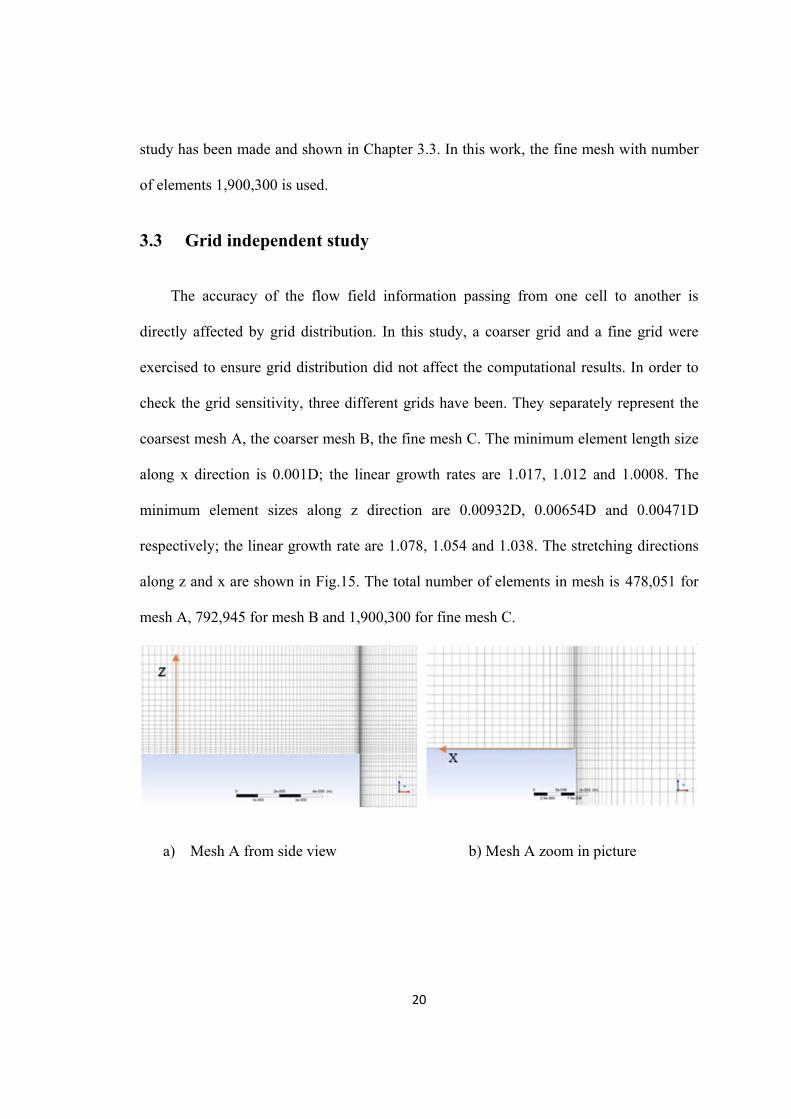
respectively; the linear growth rate are 1.078, 1.054 and 1.038. The stretching directions

along z and x are shown in Fig.15. The total number of elements in mesh is  478,051 for

mesh A, 792,945 for mesh B and 1,900,300 for fine mesh C.

a) Mesh A from side view b) Mesh A zoom in picture

21  

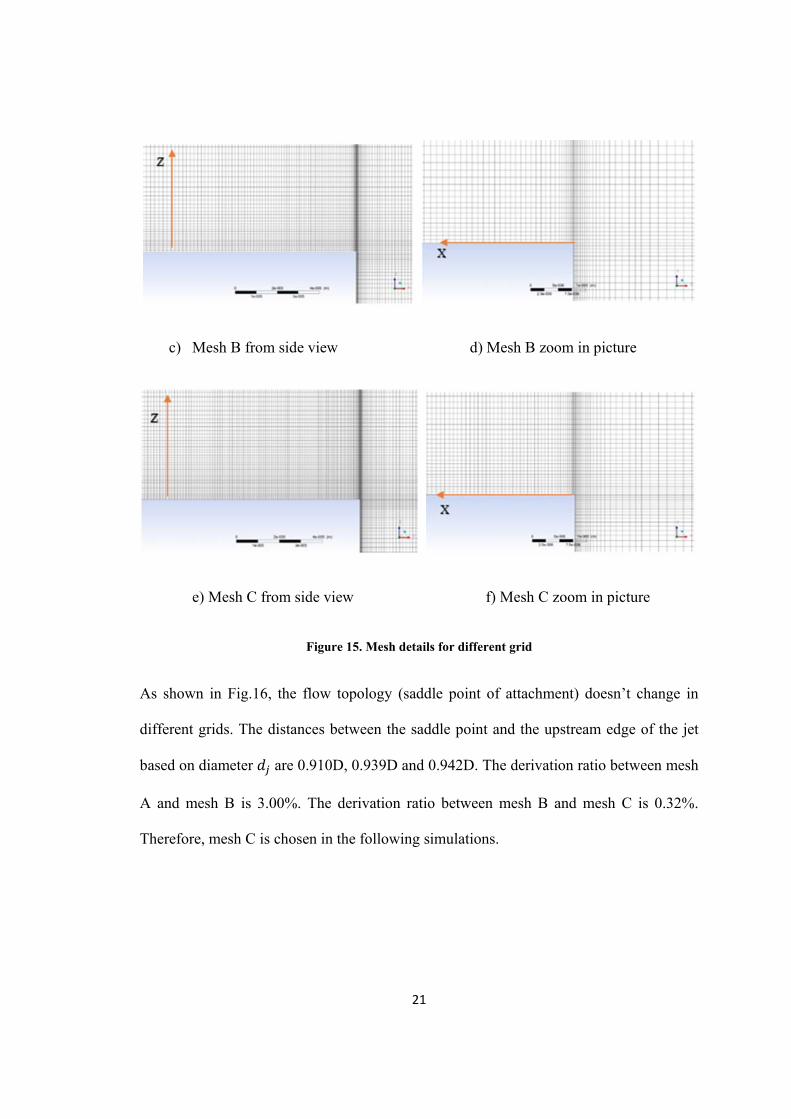
c) Mesh B from side view d) Mesh B zoom in picture

e) Mesh C from side view f) Mesh C zoom in picture

Figure 15. Mesh details for different grid

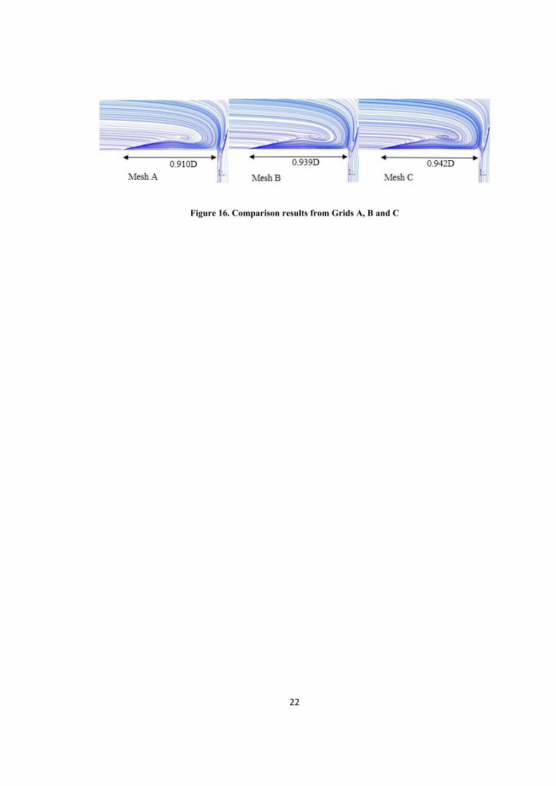
As shown in Fig.16, the flow topology (saddle point of attachment) doesn’t change in

different grids. The distances between the saddle point and the upstream edge of the jet

based on diameter are 0.910D, 0.939D and 0.942D. The derivation ratio between mesh

A and mesh B is 3.00%. The derivation ratio between mesh B and mesh C is 0.32%.

Therefore, mesh C is chosen in the following simulations.

22  

Figure 16. Comparison results from Grids A, B and C

23  

Chapter 4 RESULTS AND DISCUSSION

In this chapter, the new flow topology is found for the crossflow with jet and verified by

mathematical analysis and topology rules after validating the numerical results with

juncture flow [21]. The effects of the velocity ratio, the crossflow boundary layer

thickness and the oscillation of the jet on the upstream topologies and the locations of

singular point are discussed.

4.1 Validation with juncture flow

There have been several work focused on an investigation of outermost singular

point in juncture flow [19, 21-23]. To validate the accuracy of numerical simulation and

ensure appropriate mesh distribution, laminar juncture flow is simulated before exploring

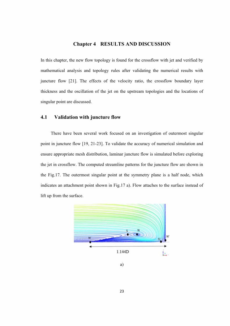
the jet in crossflow. The computed streamline patterns for the juncture flow are shown in

the Fig.17. The outermost singular point at the symmetry plane is a half node, which

indicates an attachment point shown in Fig.17 a). Flow attaches to the surface instead of

lift up from the surface.

a)

24  

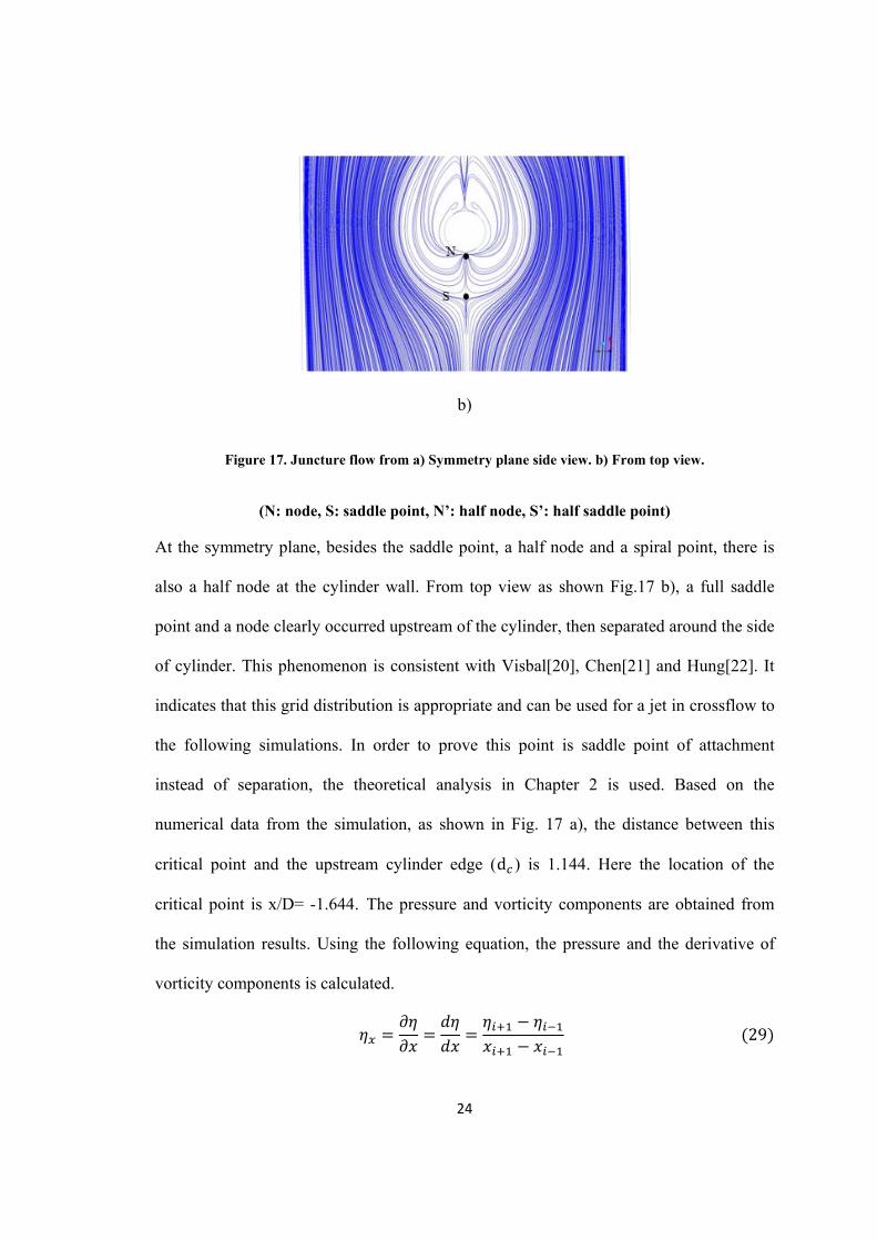
b)

Figure 17. Juncture flow from a) Symmetry plane side view. b) From top view.

(N: node, S: saddle point, N’: half node, S’: half saddle point)

At the symmetry plane, besides the saddle point, a half node and a spiral point, there is

also a half node at the cylinder wall. From top view as shown Fig.17 b), a full saddle

point and a node clearly occurred upstream of the cylinder, then separated around the side

of cylinder. This phenomenon is consistent with Visbal[20], Chen[21] and Hung[22]. It

indicates that this grid distribution is appropriate and can be used for a jet in crossflow to

the following simulations. In order to prove this point is saddle point of attachment

instead of separation, the theoretical analysis in Chapter 2 is used. Based on the

numerical data from the simulation, as shown in Fig. 17 a), the distance between this

critical point and the upstream cylinder edge (d ) is 1.144. Here the location of the

critical point is x/D= -1.644. The pressure and vorticity components are obtained from

the simulation results. Using the following equation, the pressure and the derivative of

vorticity components is calculated.

29

25  

ξξ ξ ξ ξ

30

PP P P

31

The cell unit is 0.0001D. Therefore,

212

32 η 0.091 32

The angle of attachment is 6.68 degree. The angle is about 10.45 degree in the

numerical results which is consistent with the theoretical analysis. Based on the results of

calculation, the derivative of vorticity components ratio is

0.617 1 33

According to the discussion in chapter 2, if the ratio is less than 1, this singular point at

y=0 plane has to be a node. It is confirmed that the outermost singular point is a saddle

point of attachment.

4.2 Jet in crossflow with different velocity ratios

To study the effects of velocity ratios at different boundary layer thicknesses, d is given

20D and 1.6D, the velocity ratio is 1.5, 2 and 2.5.

4.2.1 Results for d=20D

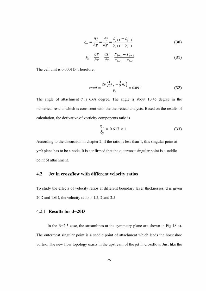
In the R=2.5 case, the streamlines at the symmetry plane are shown in Fig.18 a).

The outermost singular point is a saddle point of attachment which leads the horseshoe

vortex. The new flow topology exists in the upstream of the jet in crossflow. Just like the

26  

juncture flow, the main boundary layer of the incoming flow aggregates and forms a

spiral point(N), then goes around the jet. However, the lower portion of the boundary

layer flow goes toward the saddle point(S) and eventually turns to the half node at the flat

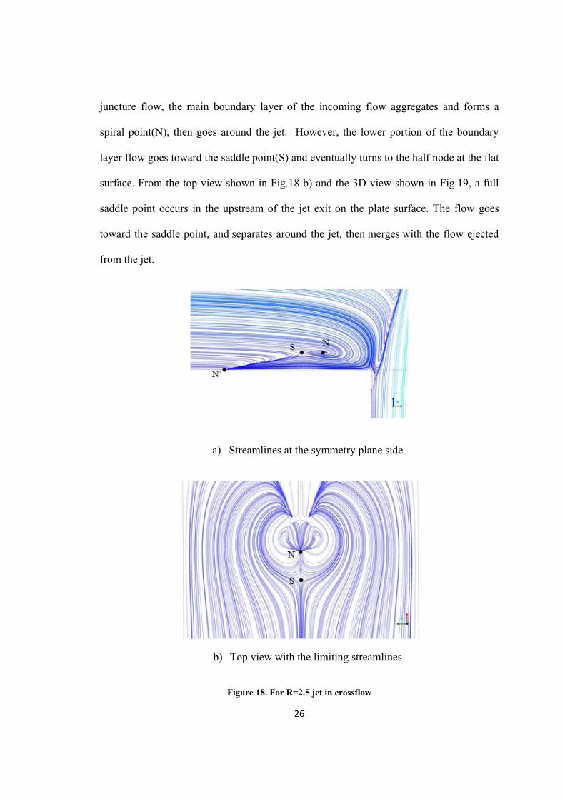
surface. From the top view shown in Fig.18 b) and the 3D view shown in Fig.19, a full

saddle point occurs in the upstream of the jet exit on the plate surface. The flow goes

toward the saddle point, and separates around the jet, then merges with the flow ejected

from the jet.

a) Streamlines at the symmetry plane side

b) Top view with the limiting streamlines

Figure 18. For R=2.5 jet in crossflow

27  

Figure 19. 3D view for jet in crossflow

The location of the attachment point x/D is -1.442. Based on the mathematical theory and

data from numerical results,

212

32 η 0.159 34

The angle of attachment is 9.01 degree. From the numerical simulation results, the

angle is about 11.60 degree. Hence, the theoretical analysis and numerical results are in

good agreement. Furthermore, the derivative of vorticity components ratio is

0.712 1, 35

so the existence of node at the symmetry plane is proved.

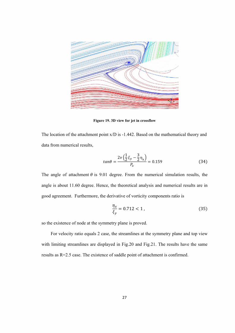
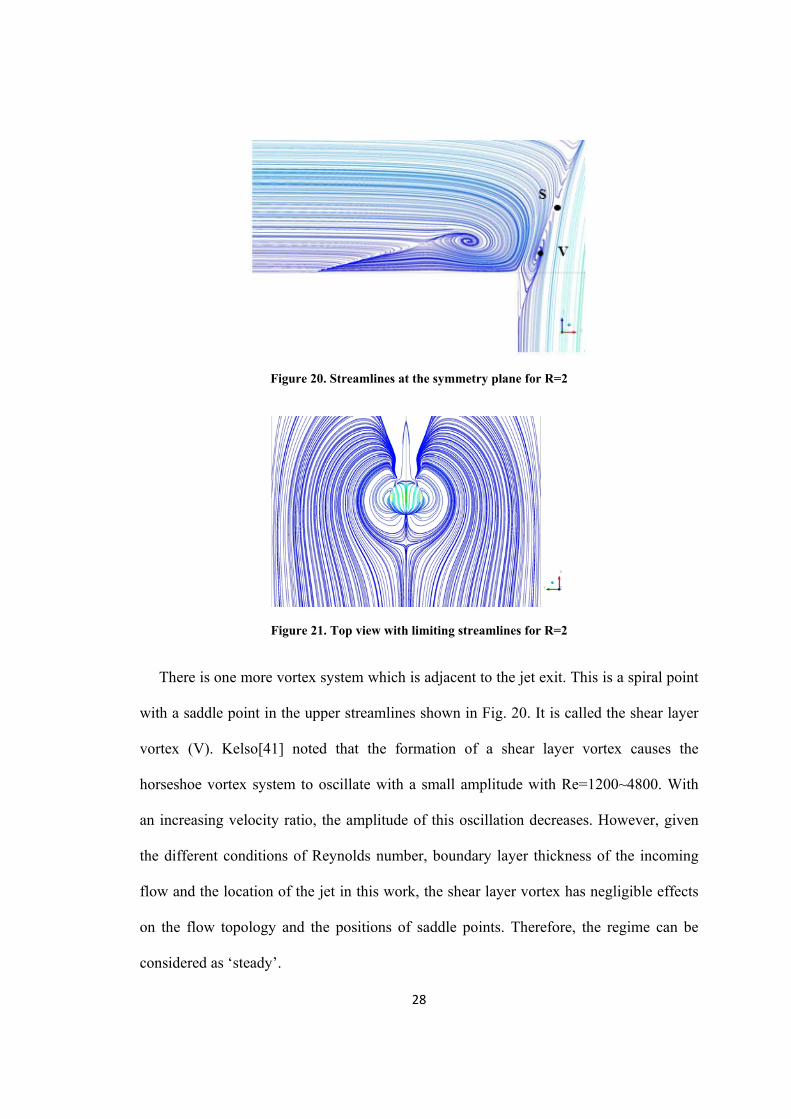
For velocity ratio equals 2 case, the streamlines at the symmetry plane and top view

with limiting streamlines are displayed in Fig.20 and Fig.21. The results have the same

results as R=2.5 case. The existence of saddle point of attachment is confirmed.

28  

Figure 20. Streamlines at the symmetry plane for R=2

Figure 21. Top view with limiting streamlines for R=2

There is one more vortex system which is adjacent to the jet exit. This is a spiral point

with a saddle point in the upper streamlines shown in Fig. 20. It is called the shear layer

vortex (V). Kelso[41] noted that the formation of a shear layer vortex causes the

horseshoe vortex system to oscillate with a small amplitude with Re=1200~4800. With

an increasing velocity ratio, the amplitude of this oscillation decreases. However, given

the different conditions of Reynolds number, boundary layer thickness of the incoming

flow and the location of the jet in this work, the shear layer vortex has negligible effects

on the flow topology and the positions of saddle points. Therefore, the regime can be

considered as ‘steady’.

29  

Beside the Reynolds number decreases to 1000 due to the lower ratio, the location of the

outermost singular point is changed. Comparing to R=2.5, in this case the location of this

half node moves forward to the jet exit. Based on the simulation results, it occurs at x/D=

-1.428, then

0.176, 0.770 1 36

The angles of attachment is 10.02. From the numerical simulation results, the angles is

12.52 degree, which matches the analytical solution well. The derivative of vorticity ratio

is less than one, which illustrates the singular points is the saddle point of attachment.

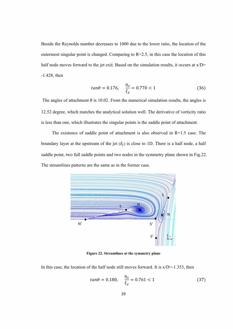
The existence of saddle point of attachment is also observed in R=1.5 case. The

boundary layer at the upstream of the jet ( ) is close to 1D. There is a half node, a half

saddle point, two full saddle points and two nodes in the symmetry plane shown in Fig.22.

The streamlines patterns are the same as in the former case.

Figure 22. Streamlines at the symmetry plane

In this case, the location of the half node still moves forward. It is x/D=-1.353, then

0.180, 0.761 1 37

30  

The angles of attachment is 10.23. From the numerical simulation results, the angles is

13.12 degree which is in agreement with mathematical analysis. Compared with former

cases, although the vorticity ratio increases with decreasing the velocity ratio, the critical

points are still the attachment points. Location of the outermost singular point keeps

moving toward the jet and the topology angle increases slightly while R is reduced.

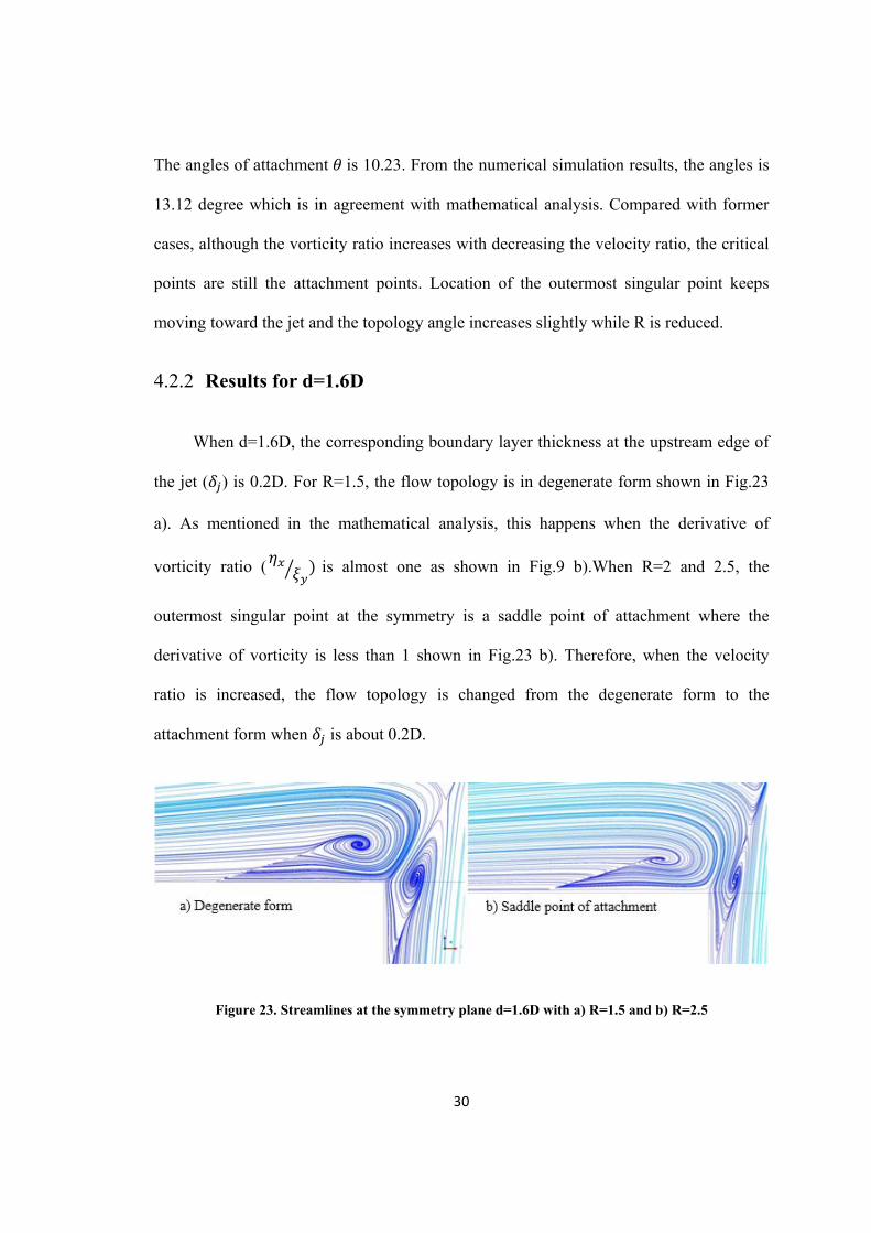
4.2.2 Results for d=1.6D

When d=1.6D, the corresponding boundary layer thickness at the upstream edge of

the jet ( ) is 0.2D. For R=1.5, the flow topology is in degenerate form shown in Fig.23

a). As mentioned in the mathematical analysis, this happens when the derivative of

vorticity ratio ( is almost one as shown in Fig.9 b).When R=2 and 2.5, the

outermost singular point at the symmetry is a saddle point of attachment where the

derivative of vorticity is less than 1 shown in Fig.23 b). Therefore, when the velocity

ratio is increased, the flow topology is changed from the degenerate form to the

attachment form when is about 0.2D.

Figure 23. Streamlines at the symmetry plane d=1.6D with a) R=1.5 and b) R=2.5

31  

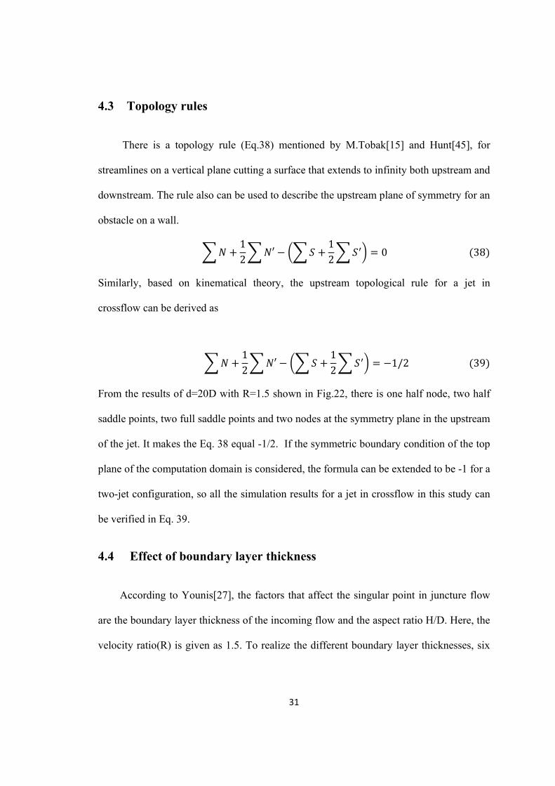
4.3 Topology rules

There is a topology rule (Eq.38) mentioned by M.Tobak[15] and Hunt[45], for

streamlines on a vertical plane cutting a surface that extends to infinity both upstream and

downstream. The rule also can be used to describe the upstream plane of symmetry for an

obstacle on a wall.

12

′12

0 38

Similarly, based on kinematical theory, the upstream topological rule for a jet in

crossflow can be derived as

12

′12

1/2 39

From the results of d=20D with R=1.5 shown in Fig.22, there is one half node, two half

saddle points, two full saddle points and two nodes at the symmetry plane in the upstream

of the jet. It makes the Eq. 38 equal -1/2. If the symmetric boundary condition of the top

plane of the computation domain is considered, the formula can be extended to be -1 for a

two-jet configuration, so all the simulation results for a jet in crossflow in this study can

be verified in Eq. 39.

4.4 Effect of boundary layer thickness

According to Younis[27], the factors that affect the singular point in juncture flow

are the boundary layer thickness of the incoming flow and the aspect ratio H/D. Here, the

velocity ratio(R) is given as 1.5. To realize the different boundary layer thicknesses, six

32  

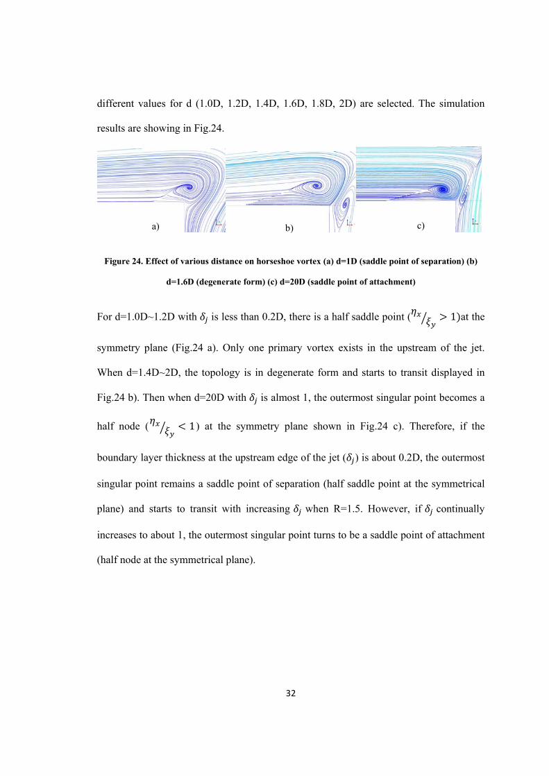
different values for d (1.0D, 1.2D, 1.4D, 1.6D, 1.8D, 2D) are selected. The simulation

results are showing in Fig.24.

Figure 24. Effect of various distance on horseshoe vortex (a) d=1D (saddle point of separation) (b)

d=1.6D (degenerate form) (c) d=20D (saddle point of attachment)

For d=1.0D~1.2D with is less than 0.2D, there is a half saddle point ( 1 at the

symmetry plane (Fig.24 a). Only one primary vortex exists in the upstream of the jet.

When d=1.4D~2D, the topology is in degenerate form and starts to transit displayed in

Fig.24 b). Then when d=20D with is almost 1, the outermost singular point becomes a

half node ( 1) at the symmetry plane shown in Fig.24 c). Therefore, if the

boundary layer thickness at the upstream edge of the jet ( ) is about 0.2D, the outermost

singular point remains a saddle point of separation (half saddle point at the symmetrical

plane) and starts to transit with increasing when R=1.5. However, if continually

increases to about 1, the outermost singular point turns to be a saddle point of attachment

(half node at the symmetrical plane).

a) b) c)

33  

4.5 Effects of oscillation

In previous cases, negligible effects on the upstream flow topology due to the shear

layer vortex are found at a constant velocity ratio. In this section, an oscillating

perturbation is applied on the jet with a certain frequency as shown in Eq. 40.

sin 2ωt , ω2

40

If Eq.40 turns to be a non-dimensional equation, it can be written as

sin ωt 41

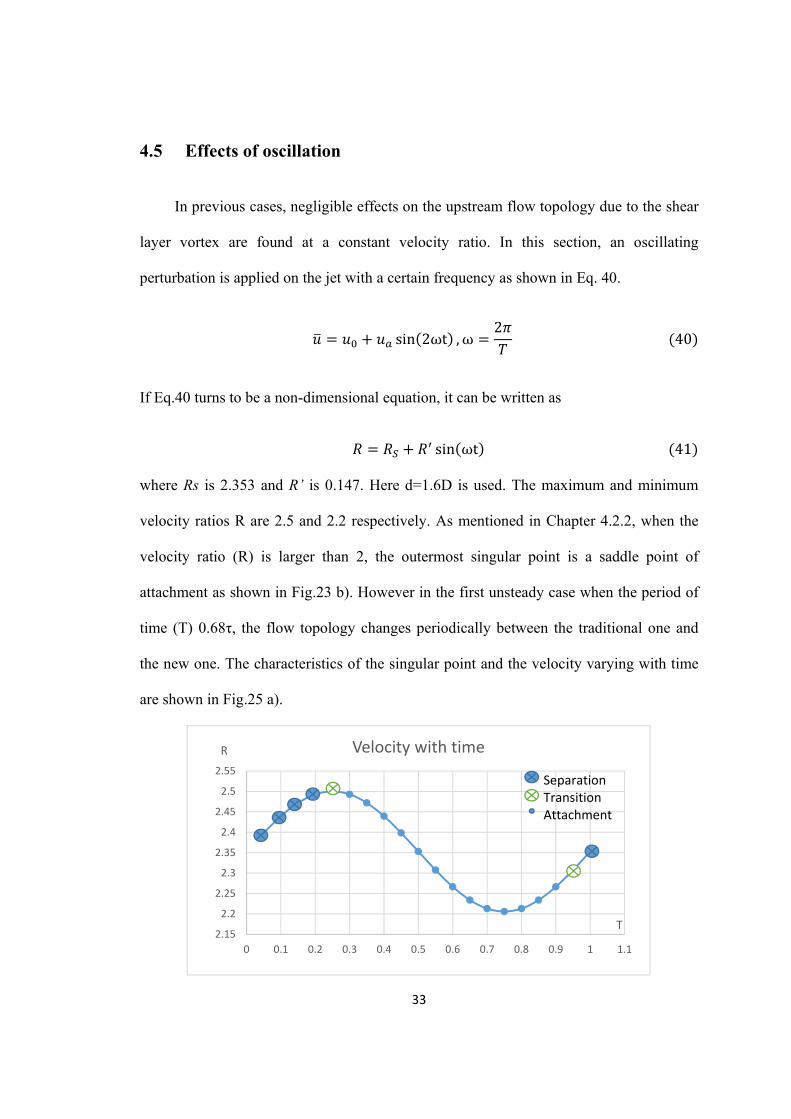
where Rs is 2.353 and R’ is 0.147. Here d=1.6D is used. The maximum and minimum

velocity ratios R are 2.5 and 2.2 respectively. As mentioned in Chapter 4.2.2, when the

velocity ratio (R) is larger than 2, the outermost singular point is a saddle point of

attachment as shown in Fig.23 b). However in the first unsteady case when the period of

time (T) 0.68τ, the flow topology changes periodically between the traditional one and

the new one. The characteristics of the singular point and the velocity varying with time

are shown in Fig.25 a).

2.15

2.2

2.25

2.3

2.35

2.4

2.45

2.5

2.55

0 0.1 0.2 0.3 0.4 0.5 0.6 0.7 0.8 0.9 1 1.1

R

T

Velocity with time

SeparationTransitionAttachment

34  

a) T= 0.68τ

 

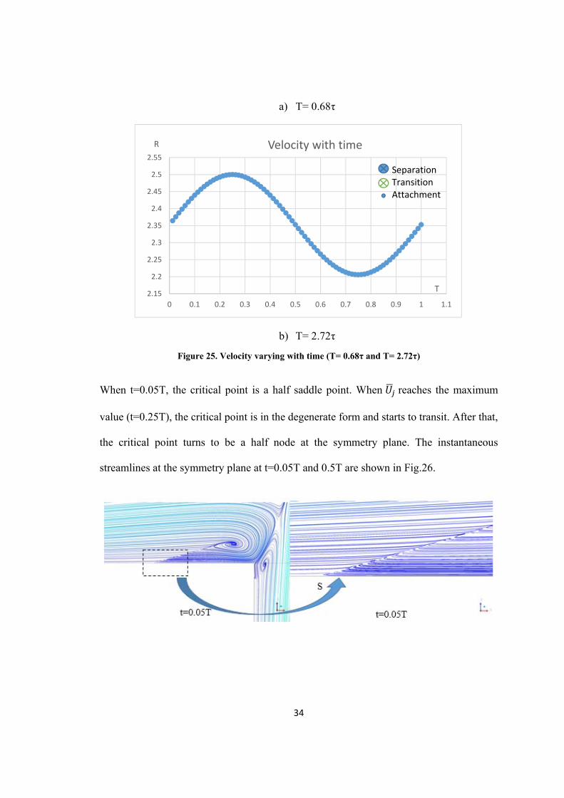
b) T= 2.72τ

Figure 25. Velocity varying with time (T= 0.68τ and T= 2.72τ)

When t=0.05T, the critical point is a half saddle point. When reaches the maximum

value (t=0.25T), the critical point is in the degenerate form and starts to transit. After that,

the critical point turns to be a half node at the symmetry plane. The instantaneous

streamlines at the symmetry plane at t=0.05T and 0.5T are shown in Fig.26.

 

2.15

2.2

2.25

2.3

2.35

2.4

2.45

2.5

2.55

0 0.1 0.2 0.3 0.4 0.5 0.6 0.7 0.8 0.9 1 1.1

R

T

Velocity with time

SeparationTransitionAttachment

35  

 

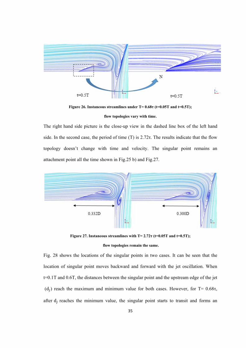
Figure 26. Instaneous streamlines under T= 0.68τ (t=0.05T and t=0.5T);

flow topologies vary with time.

The right hand side picture is the close-up view in the dashed line box of the left hand

side. In the second case, the period of time (T) is 2.72τ. The results indicate that the flow

topology doesn’t change with time and velocity. The singular point remains an

attachment point all the time shown in Fig.25 b) and Fig.27.

 

Figure 27. Instaneous streamlines with T= 2.72τ (t=0.05T and t=0.5T);

flow topologies remain the same.

Fig. 28 shows the locations of the singular points in two cases. It can be seen that the

location of singular point moves backward and forward with the jet oscillation. When

t=0.1T and 0.6T, the distances between the singular point and the upstream edge of the jet

(d ) reach the maximum and minimum value for both cases. However, for T= 0.68τ,

after d reaches the minimum value, the singular point starts to transit and forms an

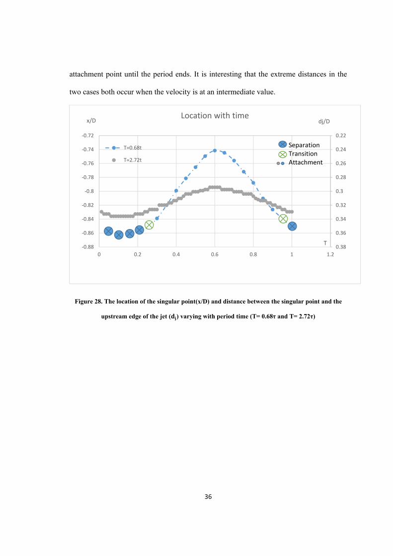
36  

attachment point until the period ends. It is interesting that the extreme distances in the

two cases both occur when the velocity is at an intermediate value.

 

Figure 28. The location of the singular point(x/D) and distance between the singular point and the

upstream edge of the jet ( ) varying with period time (T= 0.68τ and T= 2.72τ)

 

0.22

0.24

0.26

0.28

0.3

0.32

0.34

0.36

0.38‐0.88

‐0.86

‐0.84

‐0.82

‐0.8

‐0.78

‐0.76

‐0.74

‐0.72

0 0.2 0.4 0.6 0.8 1 1.2

dj/Dx/D

T

Location with time

T=0.68t

T=2.72t

SeparationTransitionAttachment

37  

Chapter 5 CONCLUSION

Numerical simulations and theoretical analysis of saddle point of attachment both in

the upstream of the cylinder and a jet in crossflow were studied in this thesis. The

existence of the new flow topology in the numerical results was verified by the

mathematical analysis and topology rules. It was found that the outermost singular point

in a jet-crossflow interaction can be a saddle point of attachment. By studying the effects

of the velocity ratio, crossflow boundary layer thickness and the oscillation of the jet flow,

several conclusions were drawn:

(1) If the boundary layer thickness at the upstream edge of the jet is about 1D, the flow

topology stays in the attachment form. With an increasing velocity ratio, the flow

topology is not affected, but the singular point moves away from the jet exit.

However, if the boundary layer thickness at the upstream edge of the jet is about 0.2D,

when the velocity ratio is decreasing, the critical point on the wall surface can change

from the attachment form to the degenerate form.

(2) When the boundary layer thickness is increased while the velocity ratio remains small

in value, the singular point changes from a saddle point of separation to a saddle point

of attachment.

(3) Given an oscillation with a certain frequency, the jet flow can change the singular

point from separation to attachment, but it’s more likely to happen at a higher

oscillating frequency. When a lower frequency is applied, the upstream flow topology

doesn’t change but the location of the saddle point moves forward and backward

periodically.

38  

References

[1] W.R. Briley and H. MoDonald, Computation of three-dimensional horseshoe vortex flow using the Navier-Stokes equations. The 7th International Conference on Numerical Methods in Fluids Dynamics, 1980.

[2] K.Y.M. Lai and A.H. Makomaski, Three-dimensional flow pattern upstream of a surface-mounted rectangular obstruction. Journal of Fluids Engineering, 1989. 111(4): p. 449-456.

[3] A.S.W. Thomas, The unsteady characteristics of laminar juncture flow. Physics of Fluids, 1987. 30(2): p. 283-285.

[4] R.G. Schwind, The three dimensional boundary layer near strut. Gas turbine Laboratory, 1962.

[5] B. Dargahi, The turbulent flow field around a circular cylinder Experiments in Fluids, 1989. 8(1-2): p. 1-12.

[6] C.V. Seal, et al., Quantitative characteristics of a laminar, unsteady necklace vortex system at a rectangular block-flat plate juncture. Journal of Fluid Mechanics, 1995(286): p. 117-135.

[7] C.J. Baker, The laminar horseshoe vortex. Journal of Fluid Mechanics, 1979. 95(2): p. 347-367.

[8] W.A. Eckerle and L.S. Langston, Horseshoe vortex formation around a cylinder. Journal of Turbomachinery, 1987. 109(2): p. 278-285.

[9] M.C. Thompson, K. Hourigan, and C. Scientific, Prediction of the vortex junction flow upstream of a surface mounted obstacle. 11th Australasian Fluid Mechanics Conference, 1992.

[10] M.R. Visbal, Numerical investigation of laminar juncture flows. AIAA, 1989. 89(1873).

[11] J.H. Agui and J. Andreopoulos, Experimental investigation of a three-dimensional boundary layer flow in the vicinity of an upright wall mounted cylinder. Journal of Fluids Engineering, 1992. 114(4): p. 566.

39  

[12] T.J. Praisner and C.R. Smith, The dynamics of the horseshoe Vortex and Assiociated endwall heat transfer- Part II: Time-mean results. Journal of Turbomachinery, 2005. 128(4): p. 775-762.

[13] D.R. Sabatino and C.R. Smith, Boundary layer influence on the unsteady horseshoe vortex flow and surface heat transfer. Journal of Turbomachinery, 2009. 131(1): p. 011015.

[14] D.J. Peake and M. Tobak, Three-dimensional interactions and vortical flows with emphasis on high speeds. Vol. 252. 1980, France: North Atlantic Treaty Organization. 219.

[15] M. Tobak and D.J. Peake, Topology of three-dimensional separated flows. Annual review of fluid mechanics, 1982. 14: p. 61-85.

[16] A.E. Perry and M.S. Chong, A description of eddying motions and flow patterns using critical-point concepts. Annual review of fluid mechanics, 1987. 19: p. 125-155.

[17] J.L. Helman and L. Hesselink, Visualizing vector field topology in fluid flows. IEEE Computer Graphics and Applications, 1991. 8(3): p. 36-46.

[18] M.S. Chong, A.E. Perry, and B.J. Cantwell, A general classification of three-dimensional flow fields. Physics of Fluids, 1990. 2(5): p. 765.

[19] H. Zhang, B. Hu, and M.Y. Younis, Investigation on existence and evolution of attachment saddle point structure of 3-D separation in juncture flow, in Applied Sciences and Technology 2011, IEEE: Islamabad. p. 247-253.

[20] M.R. Visbal, Structure of laminar juncture flows. AIAA, 1991. 29(8): p. 1273-1282.

[21] C.-L. Chen and C.-M. Hung, Numerical study of juncture flows. AIAA, 1992. 30(7): p. 1800-1807.

[22] C.-M. Hung, C.-H. Sung, and C.-L. Chen, Computation of saddle point of attachment AIAA, 1992. 30(6): p. 8.

[23] H. Zhang, et al., Investigation of attachment saddle point structure of 3-D steady separation in laminar juncture flow using PIV. Journal of Visualization, 2012. 15(3): p. 241-252.

40  

[24] M.D. Coon and M. Tobak, Experimental study of saddle point of attachment in laminar juncture flow. AIAA, 1995. 33(12).

[25] M.J. Khan and A. Ahmed, Topological model of flow regimes in the plane of symmetry of a surface-mounted obstacle. Physics of Fluids, 2005. 17(4): p. 045101.

[26] M. Kawahashi and K. Hosoi, Beam-sweep laser speckle velocimetry. Experiments in Fluids, 1989. 8(1-2): p. 109-111.

[27] M.Y. Younis, et al., Topological evolution of laminar juncture flows under different critical parameters. Science China Technological Sciences, 2014. 57(7): p. 1342-1351.

[28] H.-C. Chen, Calculations of submarine flow by multiblock Reynolds-averaged Navier-Stokes method. Engineering Turbulence Modelling and Experiments 2, 1993: p. 711-720.

[29] S. Bagheri, et al., Global stability of a jet in cross-flow. Journal of Fluid Mechanics, 2009(624): p. 33-44.

[30] Ziefle, Jörg, and L. Kleiser, Large-eddy simulation of a round jet in crossflow. AIAA 2009: p. 1158-1172.

[31] K. Mahesh, The interaction of jets with crossflow. Annual Review of Fluid Mechanics, 2013. 45: p. 397-407.

[32] T. Cambonie and J.-L. Aider, Transition scenario of the round jet in crossflow topology at low velocity ratios. Physics of Fluids, 2014. 26: p. 084101.

[33] J.S. Shang, et al., Interaction of jet in hypersonic cross stream. AIAA, 1989. 27(3): p. 323-329.

[34] A. Krothapalli, L. Lourenco, and J. Buchlin, Separated flow upstream of a jet in a crossflow. AIAA, 1990. 28(3): p. 414.

[35] D.A. Dickmann and F.K. Lu, Shock/boundary layer interaction effects on transverse jets in crossflow over a flat plate. Journal of Spacecraft and Rockets, 2009. 46.

41  

[36] A. Sau, et al., Structural development of vortical flows around a square jet in cross-flow. The Royal Society, 2004. 460(2051): p. 3339-3368.

[37] A. Sau, et al., Three-dimensional simulation of square jets in cross-flow. The American Physical Society, 2004. 69(20): p. 066302.

[38] X.D. Wang, et al., Numerical simulations of imperfect bifurcation of jet in crossflow. Engineering Applications of Computational Fluid Mechanics, 2012. 6(4): p. 595-607.

[39] E. Erdem, K. Kontis, and S. Saravanan, Penetration characteristics of air, carbon dioxide and helium transverse sonic jets in mach 5 cross flow. Sensors, 2014. 14(12): p. 23462-23489.

[40] P. Schlatter, S. Bagheri, and D.S. Henningson, Self-sustained global oscillations in a jet in crossflow. Theoretical and Computational Fluid Dynamics, 2010. 25(1-4): p. 129-146.

[41] R.M. Kelso and A.J. Smits, Horseshoe vortex systems resulting from the interaction between a laminar boundary layer and a transverse jet. Physics of Fluids, 1995. 7(1): p. 153-158.

[42] R.M. Kelso, T.T. Lim, and A.E. Perry, An experimental study of round jets in cross-flow. Journal of Fluid Mechanics, 1996. 306(1): p. 111-144.

[43] A.E. Perry and B.D. Fairlie, Critical points in flow patterns. Vol. 18. 1975: Advances in Geophysics. 299-315.

[44] E. Recker, et al., Experimental study of a round jet in cross-flow at low momentum ratio. Application of Laser Techniques to Fluid Mechanics, 2010. 05-08.

[45] J.C.R. Hunt, et al., Kinematical studies of the flows around free or surface-mounted obstacles; applying topology to flow visualization. Journal of Fluid Mechanics, 1978. 86(1): p. 179-200.