Embed Size (px)
Citation preview
National Aeronautics and Space Administration
Thibault Flinois, Michael Bottom, Stefan Martin, Daniel Scharf, Megan Davis, Stuart Shaklan
Jet Propulsion Laboratory, California Institute of Technology
April 4th, 2019
© 2019 California Institute of Technology. Government sponsorship acknowledged. (CL#19-1857)
S5: Starshade technology to TRL5
Milestone 4 : Lateral formation sensing & control

ExoPlanet Exploration Program
Introduction and overview
ExoPlanet Exploration Program
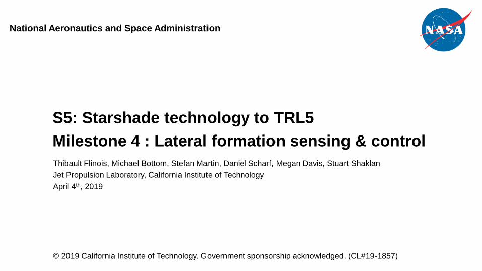
Starshades: stop the starlight from
getting into your telescope
3
Create an “artificial eclipse” using a ~30 meter flower-shaped occulter
…flying 20-80,000 km in front of your telescope
discovermagazine.com
ExoPlanet Exploration Program
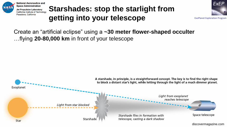
Starshades operations concept
4
1. Starshades slews to target star
2. Starshade and telescope align themselves with the target star
3. Telescope detects planets around the target star
4. GOTO: 1) until you run out of fuel
Savransky et al. 2015
ExoPlanet Exploration Program
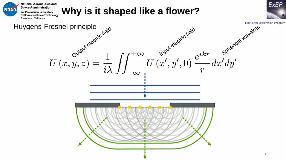
Huygens-Fresnel principle
Why is it shaped like a flower?
5
ExoPlanet Exploration Program
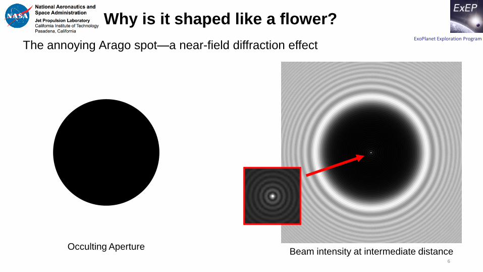
The annoying Arago spot—a near-field diffraction effect
Why is it shaped like a flower?
6
Beam intensity at intermediate distanceOcculting Aperture
ExoPlanet Exploration Program
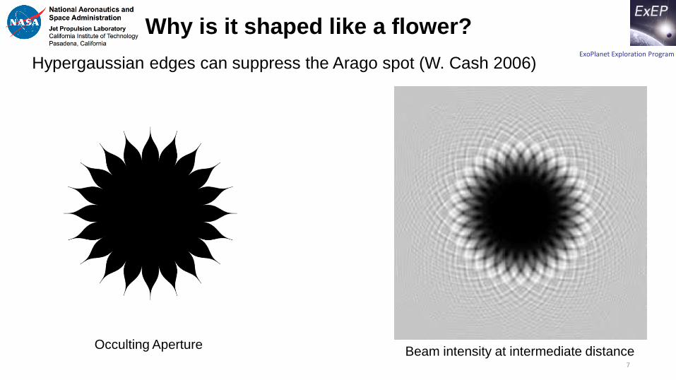
Hypergaussian edges can suppress the Arago spot (W. Cash 2006)
Why is it shaped like a flower?
7
Beam intensity at intermediate distanceOcculting Aperture
ExoPlanet Exploration Program
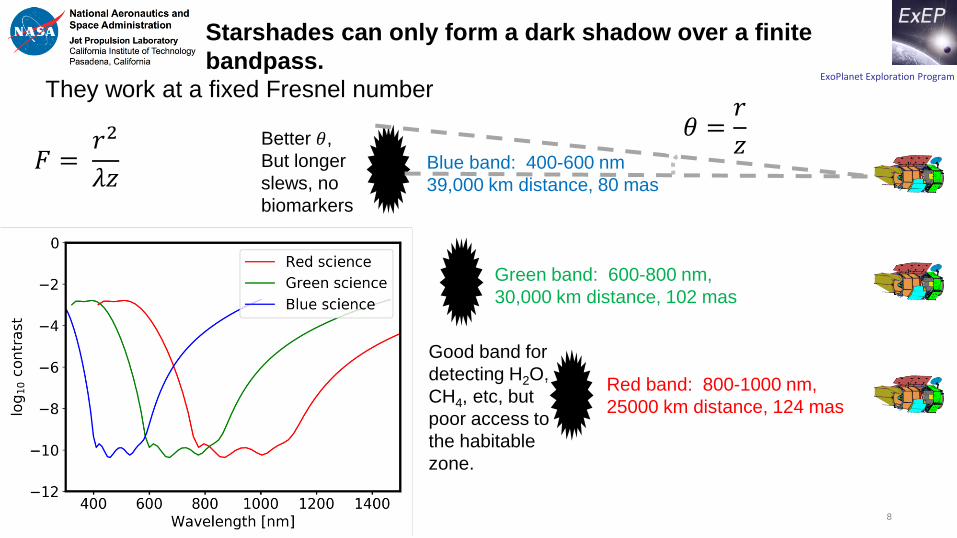
Good band for
detecting H2O,
CH4, etc, but
poor access to
the habitable
zone.
They work at a fixed Fresnel number
Starshades can only form a dark shadow over a finite
bandpass.
8
Better 𝜃,
But longer
slews, no
biomarkers
Blue band: 400-600 nm
39,000 km distance, 80 mas
Green band: 600-800 nm,
30,000 km distance, 102 mas
Red band: 800-1000 nm,
25000 km distance, 124 mas
𝜃 =𝑟
𝑧𝐹 =
𝑟2
𝜆𝑧
ExoPlanet Exploration Program
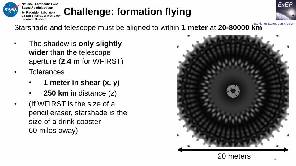
• The shadow is only slightly
wider than the telescope
aperture (2.4 m for WFIRST)
• Tolerances
• 1 meter in shear (x, y)
• 250 km in distance (z)
• (If WFIRST is the size of a
pencil eraser, starshade is the
size of a drink coaster
60 miles away)
Starshade and telescope must be aligned to within 1 meter at 20-80000 km
Challenge: formation flying
920 meters
ExoPlanet Exploration Program
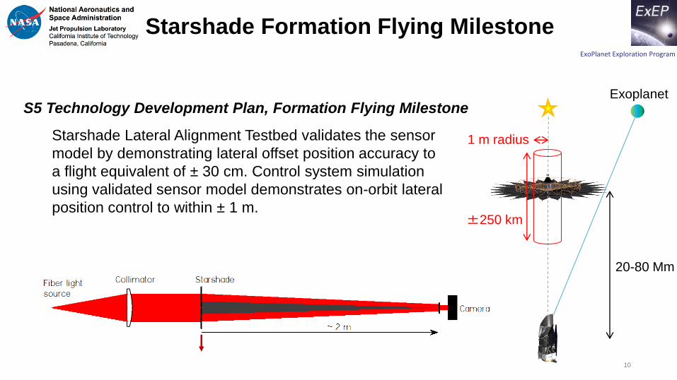
1 m radius
±250 km
Exoplanet
20-80 Mm
10
S5 Technology Development Plan, Formation Flying Milestone
Starshade Formation Flying Milestone
Starshade Lateral Alignment Testbed validates the sensor
model by demonstrating lateral offset position accuracy to
a flight equivalent of ± 30 cm. Control system simulation
using validated sensor model demonstrates on-orbit lateral
position control to within ± 1 m.
ExoPlanet Exploration Program
• Starshade Lateral Alignment Testbed validates the sensor model by
demonstrating lateral offset position accuracy to a flight equivalent of ± 30
cm– Sensor performance is demonstrated using numerical simulations and analytic model
– SLATE testbed validates the sensor model and demonstrates sensor function
• Control system simulation using validated sensor model demonstrates on-
orbit lateral position control to within ± 1 m– A high-fidelity simulation of the space environment including the testbed-validated lateral sensor
model is developed and validated
– Robust control performance is demonstrated in Monte Carlo simulations
S5 Milestone and approach to TRL5
11
ExoPlanet Exploration Program
Sensing
• Showed that the sensor performance predicted by validated simulations meets
requirement with large margin
– To reveal the sensor error, had to increase the stellar magnitudes by more than 2 and 4, thus
the sensor was given a signal between 12x and 75x fainter than expected
• Validated the end-to-end sensing approach with results from the testbed
– Testbed matched conservative (faint) SNR from flight simulations
Control
• Developed a high-fidelity simulation environment including testbed-validated lateral
sensor model
• Demonstrated control of the starshade with the required accuracy over a realistic
observation timescale
– To demonstrate robust control, the sensor error was inflated far above the expected value to
the flight equivalent of ± 30 cm called for in the milestone statement
Milestone: Results Brief
12
ExoPlanet Exploration Program
Lateral sensing
ExoPlanet Exploration Program
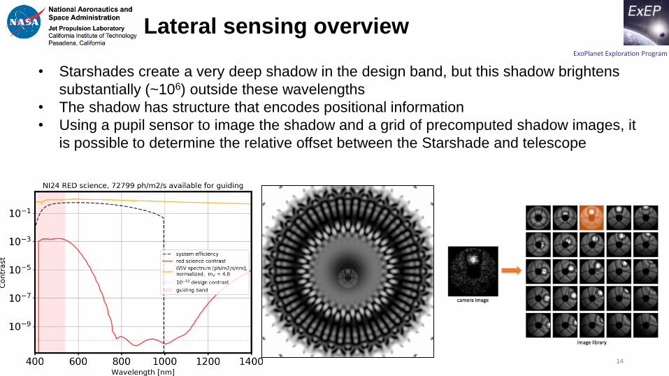
Lateral sensing overview
14
• Starshades create a very deep shadow in the design band, but this shadow brightens
substantially (~106) outside these wavelengths
• The shadow has structure that encodes positional information
• Using a pupil sensor to image the shadow and a grid of precomputed shadow images, it
is possible to determine the relative offset between the Starshade and telescope
ExoPlanet Exploration Program
15
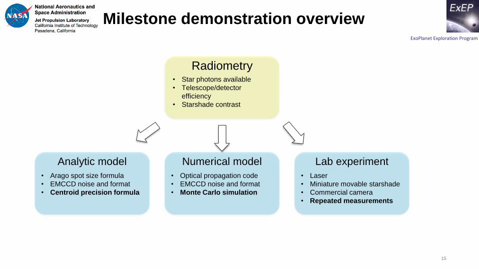
Radiometry• Star photons available
• Telescope/detector
efficiency
• Starshade contrast
Analytic model
• Arago spot size formula
• EMCCD noise and format
• Centroid precision formula
Numerical model
• Optical propagation code
• EMCCD noise and format
• Monte Carlo simulation
Lab experiment
• Laser
• Miniature movable starshade
• Commercial camera
• Repeated measurements
Milestone demonstration overview
ExoPlanet Exploration Program
• A key question is how much light is detected by the pupil camera, the CGI
low-order wavefront sensor (LOWFS)
• This depends on:
– The stellar photon flux
– The starshade contrast
– The internal optical efficiency of the telescope
– The detector efficiency
• This subsection will review how these numbers are determined
Main points
Radiometry
16
ExoPlanet Exploration Program
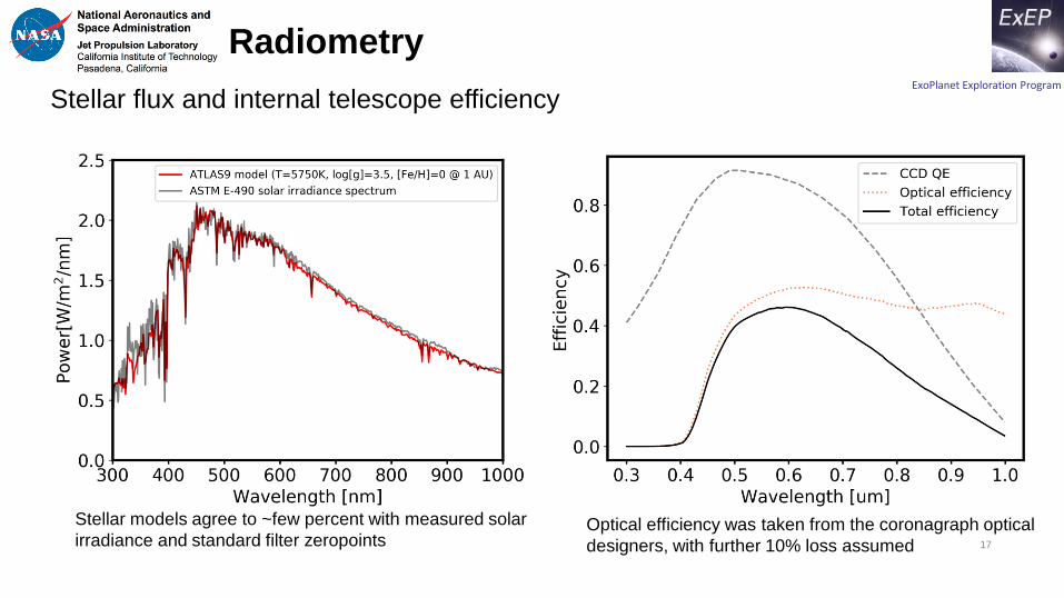
Stellar flux and internal telescope efficiency
Radiometry
17
Stellar models agree to ~few percent with measured solar
irradiance and standard filter zeropointsOptical efficiency was taken from the coronagraph optical
designers, with further 10% loss assumed
ExoPlanet Exploration Program
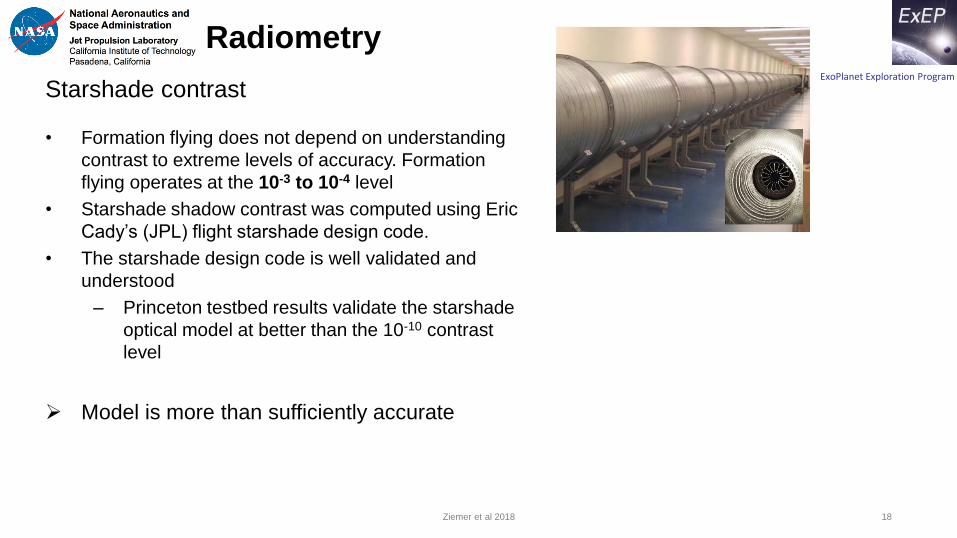
Starshade contrast
Radiometry
Ziemer et al 2018 18
• Formation flying does not depend on understanding
contrast to extreme levels of accuracy. Formation
flying operates at the 10-3 to 10-4 level
• Starshade shadow contrast was computed using Eric
Cady’s (JPL) flight starshade design code.
• The starshade design code is well validated and
understood
– Princeton testbed results validate the starshade
optical model at better than the 10-10 contrast
level
Model is more than sufficiently accurate
ExoPlanet Exploration Program
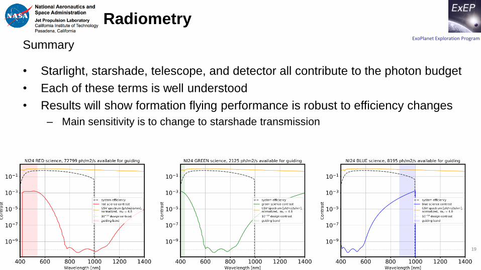
Summary
Radiometry
19
• Starlight, starshade, telescope, and detector all contribute to the photon budget
• Each of these terms is well understood
• Results will show formation flying performance is robust to efficiency changes
– Main sensitivity is to change to starshade transmission
ExoPlanet Exploration Program
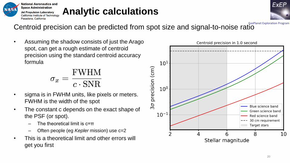
• Assuming the shadow consists of just the Arago
spot, can get a rough estimate of centroid
precision using the standard centroid accuracy
formula
• sigma is in FWHM units, like pixels or meters.
FWHM is the width of the spot
• The constant c depends on the exact shape of
the PSF (or spot).
– The theoretical limit is c=π
– Often people (eg Kepler mission) use c=2
• This is a theoretical limit and other errors will
get you first
Analytic calculations
20
Centroid precision can be predicted from spot size and signal-to-noise ratio
ExoPlanet Exploration Program
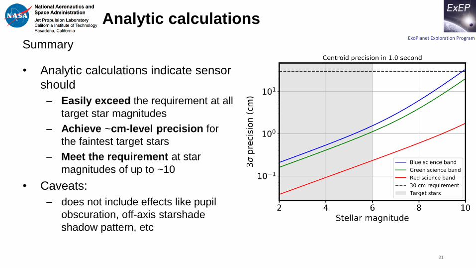
• Analytic calculations indicate sensor
should
– Easily exceed the requirement at all
target star magnitudes
– Achieve ~cm-level precision for
the faintest target stars
– Meet the requirement at star
magnitudes of up to ~10
• Caveats:
– does not include effects like pupil
obscuration, off-axis starshade
shadow pattern, etc
Summary
Analytic calculations
21
ExoPlanet Exploration Program
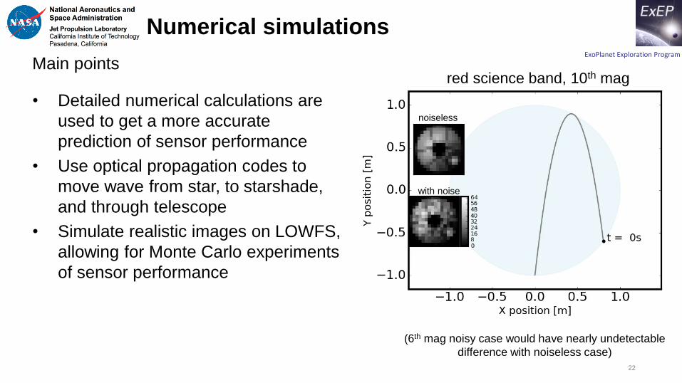
• Detailed numerical calculations are
used to get a more accurate
prediction of sensor performance
• Use optical propagation codes to
move wave from star, to starshade,
and through telescope
• Simulate realistic images on LOWFS,
allowing for Monte Carlo experiments
of sensor performance
Main points
Numerical simulations
22
red science band, 10th mag
(6th mag noisy case would have nearly undetectable
difference with noiseless case)
noiseless
with noise
ExoPlanet Exploration Program
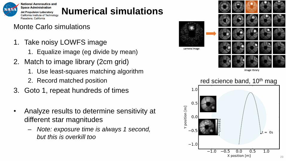
1. Take noisy LOWFS image
1. Equalize image (eg divide by mean)
2. Match to image library (2cm grid)
1. Use least-squares matching algorithm
2. Record matched position
3. Goto 1, repeat hundreds of times
• Analyze results to determine sensitivity at
different star magnitudes
– Note: exposure time is always 1 second,
but this is overkill too
Monte Carlo simulations
Numerical simulations
23
red science band, 10th mag
ExoPlanet Exploration Program
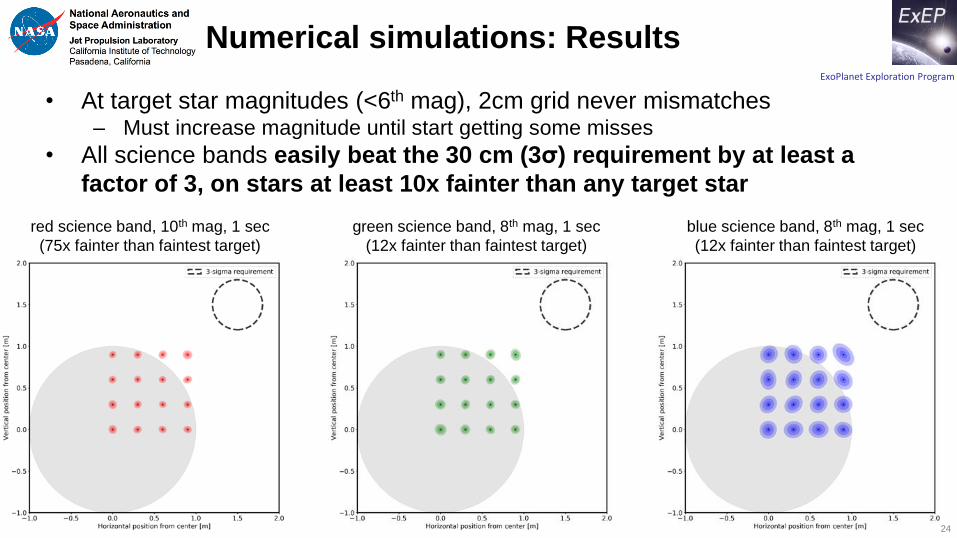
• At target star magnitudes (<6th mag), 2cm grid never mismatches– Must increase magnitude until start getting some misses
• All science bands easily beat the 30 cm (3σ) requirement by at least a
factor of 3, on stars at least 10x fainter than any target star
Numerical simulations: Results
24
red science band, 10th mag, 1 sec
(75x fainter than faintest target)
green science band, 8th mag, 1 sec
(12x fainter than faintest target)
blue science band, 8th mag, 1 sec
(12x fainter than faintest target)
ExoPlanet Exploration Program
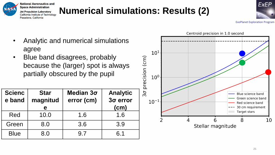
• Analytic and numerical simulations
agree
• Blue band disagrees, probably
because the (larger) spot is always
partially obscured by the pupil
Numerical simulations: Results (2)
25
Scienc
e band
Star
magnitud
e
Median 3σ
error (cm)
Analytic
3σ error
(cm)
Red 10.0 1.6 1.6
Green 8.0 3.6 3.9
Blue 8.0 9.7 6.1
ExoPlanet Exploration Program
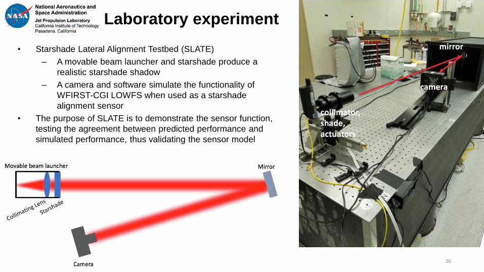
Laboratory experiment
• Starshade Lateral Alignment Testbed (SLATE)
– A movable beam launcher and starshade produce a
realistic starshade shadow
– A camera and software simulate the functionality of
WFIRST-CGI LOWFS when used as a starshade
alignment sensor
• The purpose of SLATE is to demonstrate the sensor function,
testing the agreement between predicted performance and
simulated performance, thus validating the sensor model
26
ExoPlanet Exploration Program
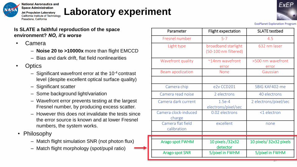
Laboratory experiment
Is SLATE a faithful reproduction of the space
environment? NO, it’s worse
• Camera
– Noise 20 to >10000x more than flight EMCCD
– Bias and dark drift, flat field nonlinearities
• Optics
– Significant wavefront error at the 10-4 contrast
level (despite excellent optical surface quality)
– Significant scatter
– Some background light/variation
– Wavefront error prevents testing at the largest
Fresnel number, by producing excess scatter.
– However this does not invalidate the tests since
the error source is known and at lower Fresnel
numbers, the system works.
• Philosophy
– Match flight simulation SNR (not photon flux)
– Match flight morphology (spot/pupil ratio)
Parameter Flight expectation SLATE testbed
Fresnel number 5-7 4.5
Light type broadband starlight (50-100 nm filtered)
632 nm laser
Wavefront quality ~14nm wavefronterror
>500 nm wavefronterror
Beam apodization None Gaussian
Camera chip e2v CCD201 SBIG KAF402-me
Camera read noise 2 electrons 40 electrons
Camera dark current 1.5e-4 electrons/pixel/sec
2 electrons/pixel/sec
Camera clock-induced charge
0.02 electrons <1 electron
Camera flat field calibration
excellent none
Arago spot FWHM 10 pixels /32x32 detector
10 pixels/ 32x32 pixels
Arago spot SNR 5/pixel in FWHM 5/pixel in FWHM
27
ExoPlanet Exploration Program
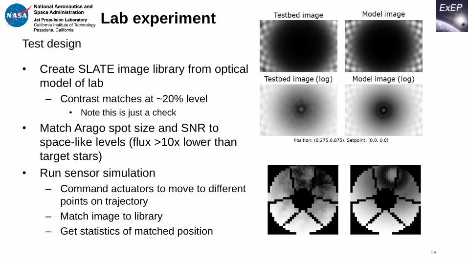
Lab experiment
• Create SLATE image library from optical
model of lab
– Contrast matches at ~20% level
• Note this is just a check
• Match Arago spot size and SNR to
space-like levels (flux >10x lower than
target stars)
• Run sensor simulation
– Command actuators to move to different
points on trajectory
– Match image to library
– Get statistics of matched position
Test design
28
ExoPlanet Exploration Program
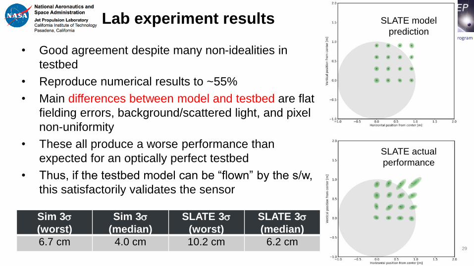
Lab experiment results
• Good agreement despite many non-idealities in
testbed
• Reproduce numerical results to ~55%
• Main differences between model and testbed are flat
fielding errors, background/scattered light, and pixel
non-uniformity
• These all produce a worse performance than
expected for an optically perfect testbed
• Thus, if the testbed model can be “flown” by the s/w,
this satisfactorily validates the sensor
Sim 3
(worst)
Sim 3
(median)
SLATE 3
(worst)
SLATE 3
(median)
6.7 cm 4.0 cm 10.2 cm 6.2 cm
SLATE model
prediction
SLATE actual
performance
29
ExoPlanet Exploration Program
Conclusions
30
1. Flight simulations predict sensor performance well above what is needed, for all
science bands, using stars ~12-75x fainter than the faintest target star
2. Laboratory experiments demonstrate good agreement with simulations of
sensor performance
ExoPlanet Exploration Program
Formation flying simulations
ExoPlanet Exploration Program
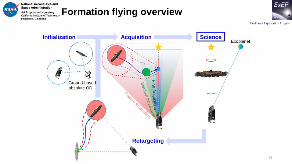
Formation flying overview
32
Acquisition Science
Retargeting
Initialization
Ground-based
absolute OD
Exoplanet
ExoPlanet Exploration Program
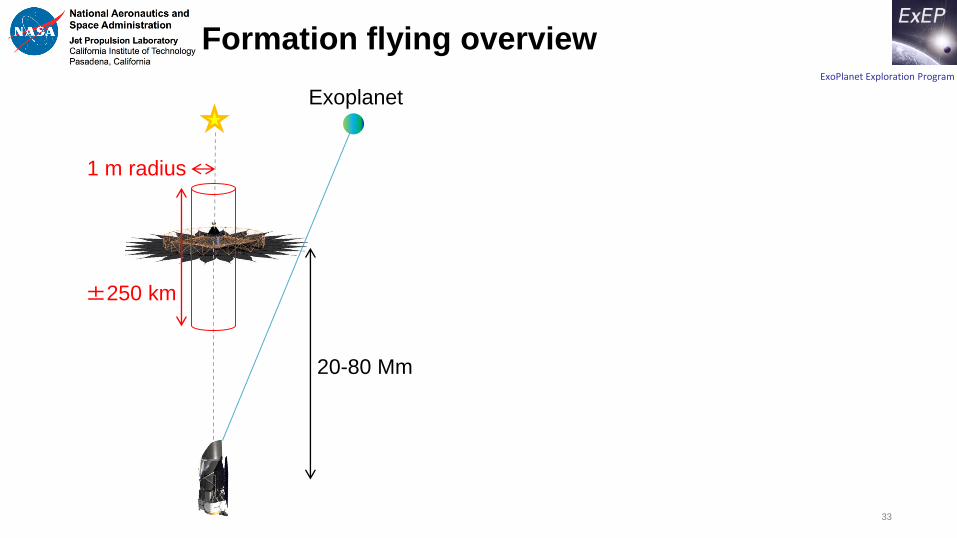
Formation flying overview
33
1 m radius
±250 km
Exoplanet
20-80 Mm
ExoPlanet Exploration Program
-1.5 -1 -0.5 0 0.5 1 1.5
y (m)
-1.5
-1
-0.5
0
0.5
1
1.5
z (
m)
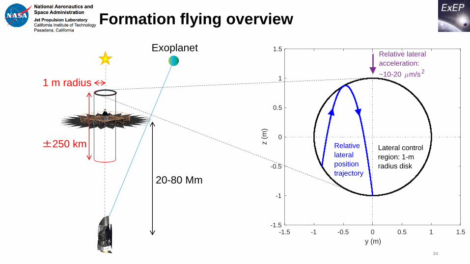
Relative
lateral
position
trajectory
Lateral control
region: 1-m
radius disk
Relative lateral
acceleration:
~10-20 m/s2
Formation flying overview
34
1 m radius
±250 km
Exoplanet
20-80 Mm
ExoPlanet Exploration Program
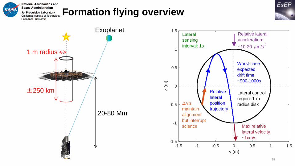
Formation flying overview
35
1 m radius
±250 km
Exoplanet
20-80 Mm
-1.5 -1 -0.5 0 0.5 1 1.5
y (m)
-1.5
-1
-0.5
0
0.5
1
1.5
z (
m)
Relative
lateral
position
trajectory
Max relative
lateral velocity
~1cm/s
v's
maintain
alignment
but interrupt
science
Relative lateral
acceleration:
~10-20 m/s2
Lateral
sensing
interval: 1s
Worst-case
expected
drift time
~900-1000s
Lateral control
region: 1-m
radius disk
ExoPlanet Exploration Program
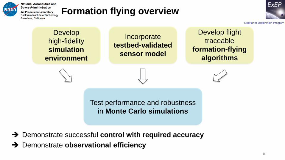
Demonstrate successful control with required accuracy
Demonstrate observational efficiency
Formation flying overview
36
Test performance and robustness
in Monte Carlo simulations
Develop
high-fidelity
simulation
environment
Incorporate
testbed-validated
sensor model
Develop flight
traceable
formation-flying
algorithms
ExoPlanet Exploration Program
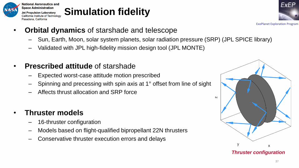
• Orbital dynamics of starshade and telescope– Sun, Earth, Moon, solar system planets, solar radiation pressure (SRP) (JPL SPICE library)
– Validated with JPL high-fidelity mission design tool (JPL MONTE)
• Prescribed attitude of starshade– Expected worst-case attitude motion prescribed
– Spinning and precessing with spin axis at 1° offset from line of sight
– Affects thrust allocation and SRP force
• Thruster models– 16-thruster configuration
– Models based on flight-qualified bipropellant 22N thrusters
– Conservative thruster execution errors and delays
Simulation fidelity
37
Thruster configuration
ExoPlanet Exploration Program
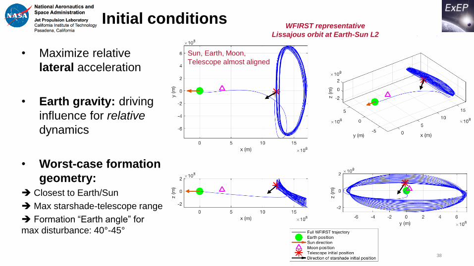
Sun, Earth, Moon,
Telescope almost aligned• Maximize relative
lateral acceleration
• Earth gravity: driving
influence for relative
dynamics
• Worst-case formation
geometry: Closest to Earth/Sun
Max starshade-telescope range
Formation “Earth angle” for
max disturbance: 40°-45°
Initial conditions
38
WFIRST representative
Lissajous orbit at Earth-Sun L2
ExoPlanet Exploration Program
-2 -1.5 -1 -0.5 0 0.5 1 1.5 2
y (m)
-2
-1.5
-1
-0.5
0
0.5
1
1.5
2
z (
m)
Control region boundary Outer threshold Inner threshold Shear positions 3 ellipses 3 requirement
-2 -1.5 -1 -0.5 0 0.5 1 1.5 2
y (m)
-2
-1.5
-1
-0.5
0
0.5
1
1.5
2
z (
m)
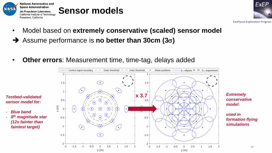
• Model based on extremely conservative (scaled) sensor model
Assume performance is no better than 30cm (3)
• Other errors: Measurement time, time-tag, delays added
Sensor models
39
Testbed-validated
sensor model for:
- Blue band
- 8th magnitude star
(12x fainter than
faintest target)
Extremely
conservative
model:
used in
formation flying
simulations
x 3.7
ExoPlanet Exploration Program
-1.5 -1 -0.5 0 0.5 1 1.5
y (m)
-1.5
-1
-0.5
0
0.5
1
1.5
z (
m)
Constant
acceleration
Final
positionInitial
position
Optimal
trajectory:
aligned with
acceleration
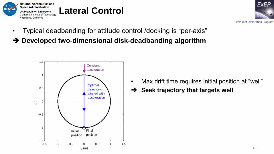
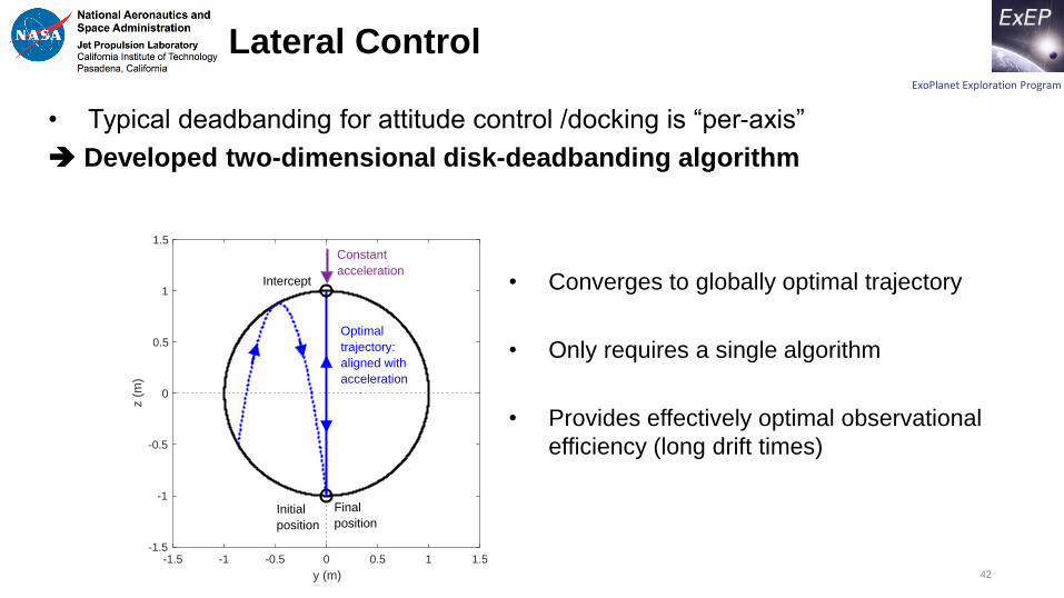
• Typical deadbanding for attitude control /docking is “per-axis”
Developed two-dimensional disk-deadbanding algorithm
Lateral Control
40
• Max drift time requires initial position at “well”
Seek trajectory that targets well
ExoPlanet Exploration Program
-1.5 -1 -0.5 0 0.5 1 1.5
y (m)
-1.5
-1
-0.5
0
0.5
1
1.5
z (
m)
Constant
acceleration
Initial
position
Intercept
Matched
slope at
intercept
Final
position
at "well"
Lateral
position
trajectory
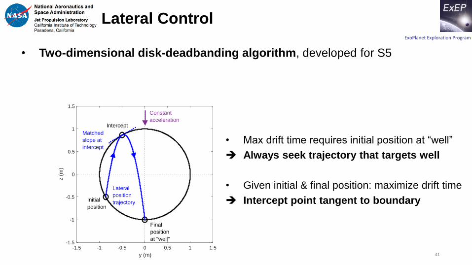
• Two-dimensional disk-deadbanding algorithm, developed for S5
Lateral Control
41
• Max drift time requires initial position at “well”
Always seek trajectory that targets well
• Given initial & final position: maximize drift time
Intercept point tangent to boundary
ExoPlanet Exploration Program
• Typical deadbanding for attitude control /docking is “per-axis”
Developed two-dimensional disk-deadbanding algorithm
Lateral Control
42
-1.5 -1 -0.5 0 0.5 1 1.5
y (m)
-1.5
-1
-0.5
0
0.5
1
1.5
z (
m)
Constant
acceleration
Final
positionInitial
position
Intercept
Optimal
trajectory:
aligned with
acceleration
• Converges to globally optimal trajectory
• Only requires a single algorithm
• Provides effectively optimal observational
efficiency (long drift times)
ExoPlanet Exploration Program
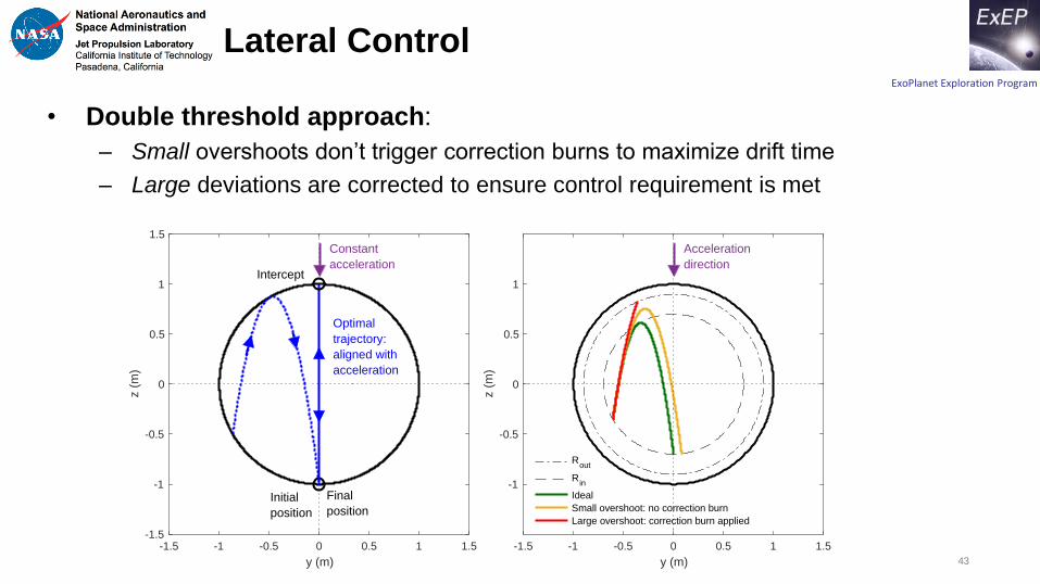
• Double threshold approach:
– Small overshoots don’t trigger correction burns to maximize drift time
– Large deviations are corrected to ensure control requirement is met
Lateral Control
43
-1.5 -1 -0.5 0 0.5 1 1.5
y (m)
-1.5
-1
-0.5
0
0.5
1
1.5
z (
m)
-1.5 -1 -0.5 0 0.5 1 1.5
y (m)
-1
-0.5
0
0.5
1
z (
m)
Rout
Rin
Ideal
Small overshoot: no correction burn
Large overshoot: correction burn applied
Constant
acceleration
Acceleration
direction
Final
positionInitial
position
Intercept
Optimal
trajectory:
aligned with
acceleration
ExoPlanet Exploration Program
• Estimation
– Filter state is 3DOF relative position, velocity, acceleration
– Constant acceleration model, justified at deadbanding timescales
• Longitudinal control
– Not required in most cases due to loose control requirement (±250km)
– Implemented “rate damping” if required: slows drift towards boundary edge
• Thrust Allocation
– Internally developed 6DOF thrust allocation algorithm used
– Developed at JPL, flight-proven e.g. used on Mars Science Laboratory
Remaining GNC algorithms
44
ExoPlanet Exploration Program
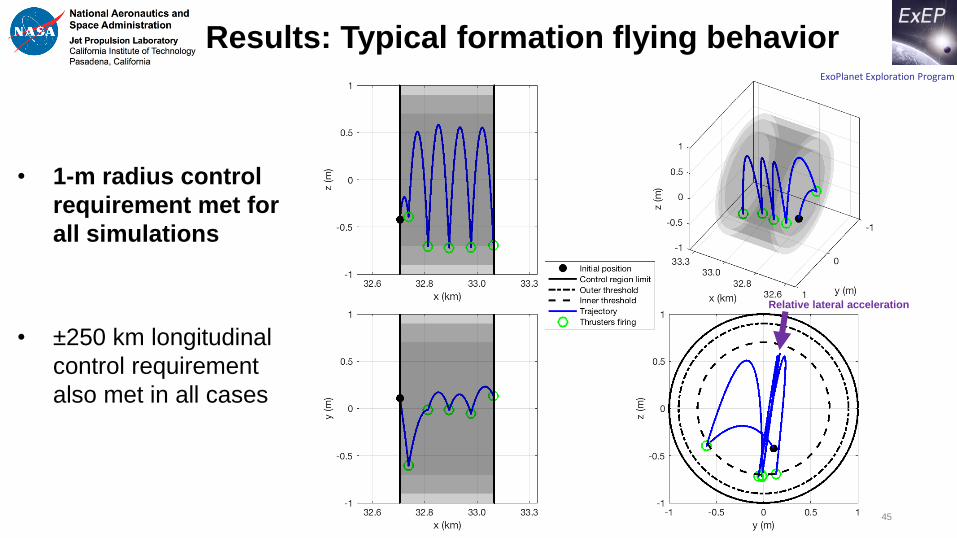
Results: Typical formation flying behavior
45
Relative lateral acceleration
• 1-m radius control
requirement met for
all simulations
• ±250 km longitudinal
control requirement
also met in all cases
ExoPlanet Exploration Program
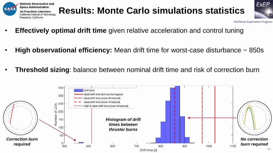
• Effectively optimal drift time given relative acceleration and control tuning
• High observational efficiency: Mean drift time for worst-case disturbance ~ 850s
• Threshold sizing: balance between nominal drift time and risk of correction burn
Results: Monte Carlo simulations statistics
46
Histogram of drift
times between
thruster burns
Correction burn
required
No correction
burn required
ExoPlanet Exploration Program
• Repeated Monte Carlo simulations with HabEx-like conditions:– Longer range (76.6Mm) ~2x larger relative lateral acceleration
– Larger dry mass (~6-7 tons)
– Worst-case HabEx initial formation geometry
Approach robust to environment
• Repeated Monte Carlo simulations 0.5Hz sensor measurement rate
Approach not driven by sensor measurements
• Identified driving disturbance: mass uncertainty– Only affects observational efficiency, not ability to meet milestone
Readily addressed with calibration
Further simulations: robustness analysis
47
ExoPlanet Exploration Program
• Showed lateral sensing approach enables formation flying for starshades
• Developed control approach that allows meeting requirements with
effectively optimal observational efficiency
• Confirmed robustness of flight-traceable GNC algorithms, even with
conservative assumptions
Formation flying simulations summary
48
ExoPlanet Exploration Program
Starshade Lateral Alignment Testbed validates the sensor model by demonstrating
lateral offset position accuracy to a flight equivalent of ± 30 cm.
Developed a lateral sensing approach based on least squares image fitting
Showed that analytical and numerical models predict excellent performance: 3x better than
requirement on 10x fainter stars
Verified and validated formation sensing technique in SLATE hardware testbed
Control system simulation using validated sensor model demonstrates on-orbit
lateral position control to within ± 1 m
Created a high-fidelity model of the flight environment including a realistic sensor model with very
conservative parameters
Developed a control approach utilizing the sensor that meets formation flying requirements with
effectively optimal observational efficiency
Confirmed robustness of flight-traceable GNC algorithms, even with conservative assumptions
Formation Flying Milestone: Conclusion

ExoPlanet Exploration Program
Questions?