Embed Size (px)
Citation preview
S3012 - Simplifying Portable Killer Apps with OpenACC and CUDA-5 Concisely and Efficiently
Rob Farber Chief Scientist, BlackDog Endeavors, LLC
Author, “CUDA Application Design and Development” Research consultant: ICHEC, Fortune 100 companies, and others
Scientist: .
Dr. Dobb’s Journal CUDA & OpenACC tutorials
• OpenCL “The Code Project” tutorials
• Columnist Scientific Computing, and other venues
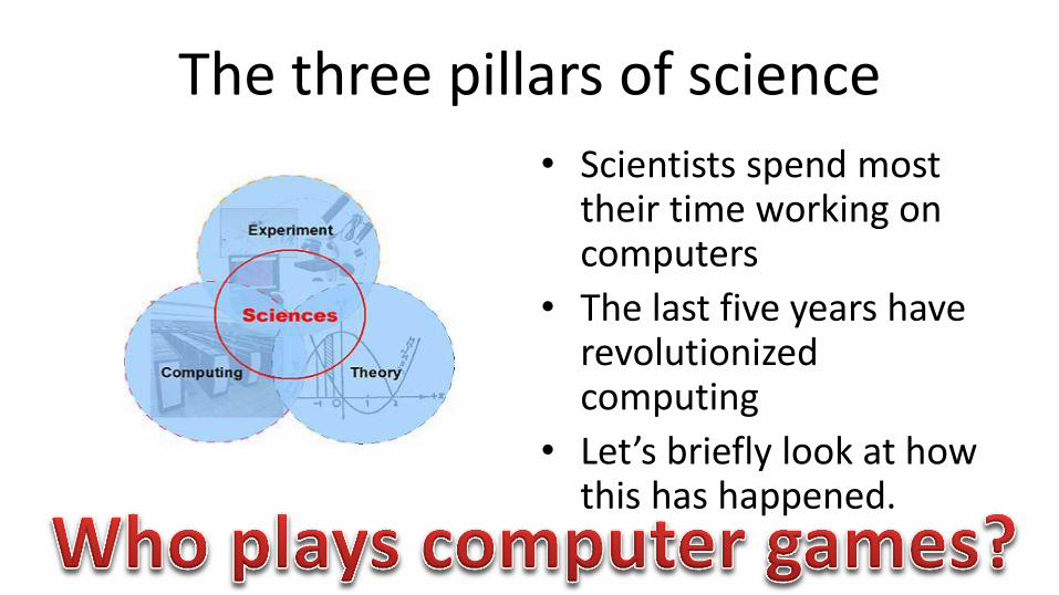
The three pillars of science
• Scientists spend most their time working on computers
• The last five years have revolutionized computing
• Let’s briefly look at how this has happened.
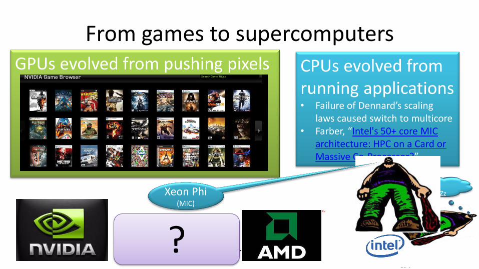
From games to supercomputers GPUs evolved from pushing pixels CPUs evolved from
running applications • Failure of Dennard’s scaling
laws caused switch to multicore • Farber, “Intel's 50+ core MIC
architecture: HPC on a Card or Massive Co-Processor?”
ZZZ
CUDA OpenCL
OpenCL
100 million+ GPUs
<mumble>
Larrabee zZz
1/3 Billion+ GPUs
Xeon Phi (MIC)
?
4
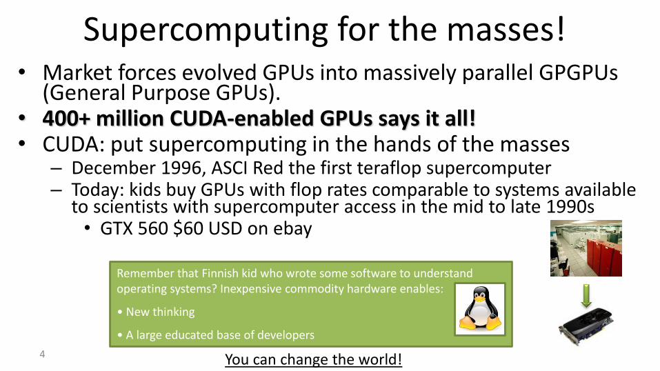
Supercomputing for the masses! • Market forces evolved GPUs into massively parallel GPGPUs
(General Purpose GPUs). • 400+ million CUDA-enabled GPUs says it all! • CUDA: put supercomputing in the hands of the masses
– December 1996, ASCI Red the first teraflop supercomputer – Today: kids buy GPUs with flop rates comparable to systems available
to scientists with supercomputer access in the mid to late 1990s • GTX 560 $60 USD on ebay
Remember that Finnish kid who wrote some software to understand operating systems? Inexpensive commodity hardware enables:
• New thinking
• A large educated base of developers
You can change the world!
5
GPUs enable killer apps! • Orders of magnitude faster apps/Low power apps:
– 10x can make computational workflows more interactive (even
poorly performing GPU apps are useful). – 100x is disruptive and has the potential to fundamentally affect
scientific research by removing time-to-discovery barriers. – 1000x and greater achieved through the use of the NVIDIA SFU
(Special Function Units) or multiple GPUs … Whooo Hoooo!
Two big ideas: 1. SIMD 2. A strong scaling execution model
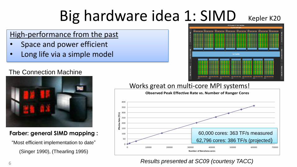
Big hardware idea 1: SIMD High-performance from the past • Space and power efficient • Long life via a simple model
Observed Peak Effective Rate vs. Number of Ranger Cores
0
50
100
150
200
250
300
350
400
0 10000 20000 30000 40000 50000 60000 70000
Number of Barcelona cores
Effe
ctiv
e Ra
te (T
F/s)
6 Results presented at SC09 (courtesy TACC)
Farber: general SIMD mapping :
“Most efficient implementation to date”
(Singer 1990), (Thearling 1995)
The Connection Machine
60,000 cores: 363 TF/s measured
62,796 cores: 386 TF/s (projected)
Works great on multi-core MPI systems!
Kepler K20
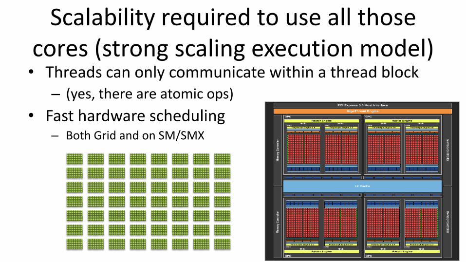
• Threads can only communicate within a thread block – (yes, there are atomic ops)
• Fast hardware scheduling – Both Grid and on SM/SMX
Scalability required to use all those cores (strong scaling execution model)
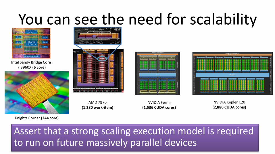
You can see the need for scalability
Assert that a strong scaling execution model is required to run on future massively parallel devices
Intel Sandy Bridge Core I7 3960X (6 core)
NVIDIA Fermi (1,536 CUDA cores)
AMD 7970 (1,280 work-item)
NVIDIA Kepler K20 (2,880 CUDA cores)
Knights Corner (244 core)
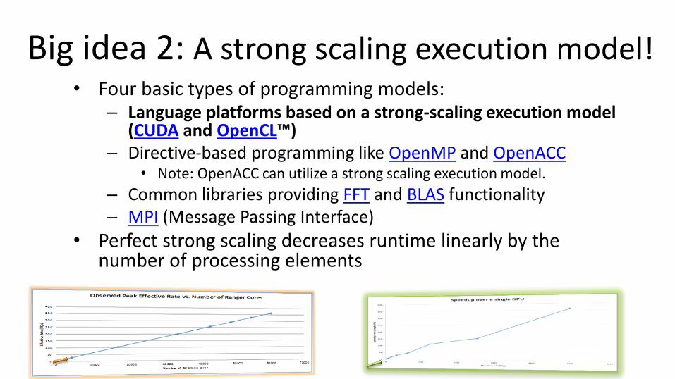
Big idea 2: A strong scaling execution model! • Four basic types of programming models:
– Language platforms based on a strong-scaling execution model (CUDA and OpenCL™)
– Directive-based programming like OpenMP and OpenACC • Note: OpenACC can utilize a strong scaling execution model.
– Common libraries providing FFT and BLAS functionality – MPI (Message Passing Interface)
• Perfect strong scaling decreases runtime linearly by the number of processing elements
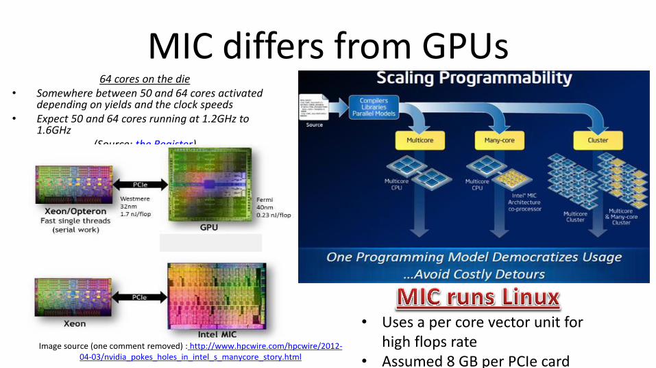
MIC differs from GPUs 64 cores on the die
• Somewhere between 50 and 64 cores activated depending on yields and the clock speeds
• Expect 50 and 64 cores running at 1.2GHz to 1.6GHz
(Source: the Register)
• Uses a per core vector unit for high flops rate
• Assumed 8 GB per PCIe card Image source (one comment removed) : http://www.hpcwire.com/hpcwire/2012-
04-03/nvidia_pokes_holes_in_intel_s_manycore_story.html
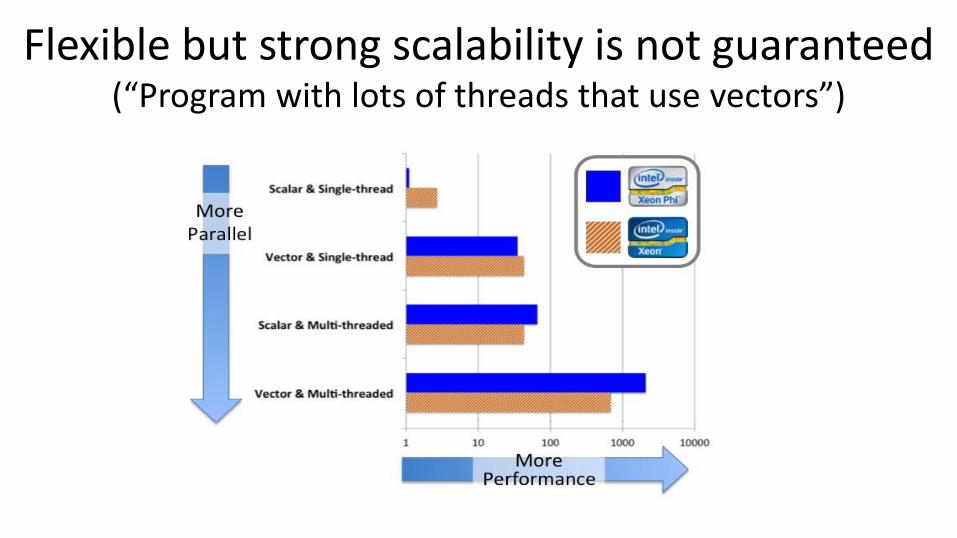
Flexible but strong scalability is not guaranteed (“Program with lots of threads that use vectors”)
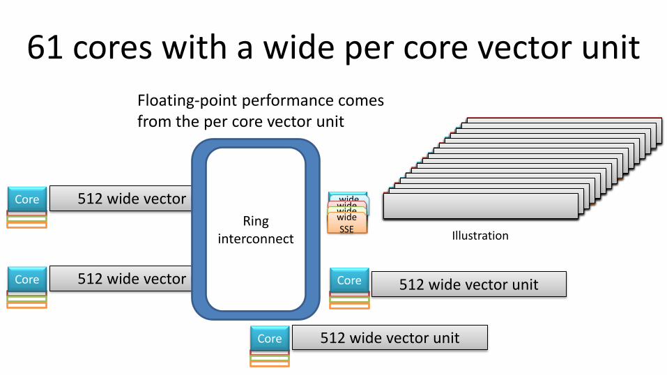
61 cores with a wide per core vector unit
Floating-point performance comes from the per core vector unit
Core wide SSE
wide SSE
wide SSE
wide SSE
Core
Core
512 wide vector unit
512 wide vector unit
Core 512 wide vector unit
Core 512 wide vector unit
Ring interconnect Illustration
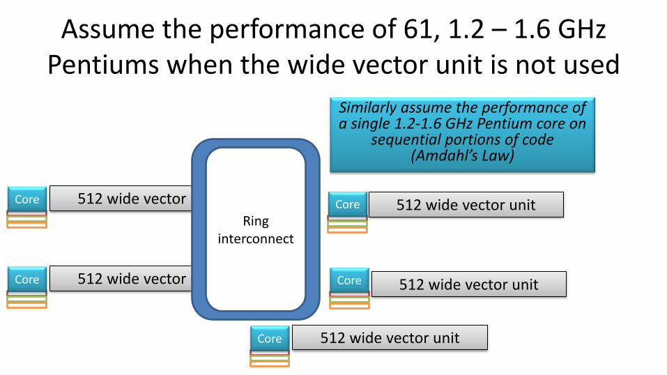
Assume the performance of 61, 1.2 – 1.6 GHz Pentiums when the wide vector unit is not used
Core
Core
Core
512 wide vector unit
512 wide vector unit
Core 512 wide vector unit
Core 512 wide vector unit
Ring interconnect
512 wide vector unit
Similarly assume the performance of a single 1.2-1.6 GHz Pentium core on
sequential portions of code (Amdahl’s Law)
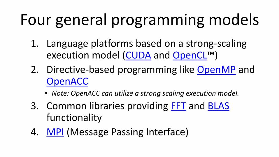
Four general programming models
1. Language platforms based on a strong-scaling execution model (CUDA and OpenCL™)
2. Directive-based programming like OpenMP and OpenACC • Note: OpenACC can utilize a strong scaling execution model.
3. Common libraries providing FFT and BLAS functionality
4. MPI (Message Passing Interface)
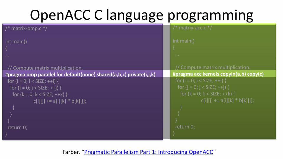
OpenACC C language programming
Farber, “Pragmatic Parallelism Part 1: Introducing OpenACC”
/* matrix-acc.c */ int main() { … // Compute matrix multiplication. #pragma acc kernels copyin(a,b) copy(c) for (i = 0; i < SIZE; ++i) { for (j = 0; j < SIZE; ++j) { for (k = 0; k < SIZE; ++k) { c[i][j] += a[i][k] * b[k][j]; } } } return 0; }
/* matrix-omp.c */ int main() { … // Compute matrix multiplication. #pragma omp parallel for default(none) shared(a,b,c) private(i,j,k) for (i = 0; i < SIZE; ++i) { for (j = 0; j < SIZE; ++j) { for (k = 0; k < SIZE; ++k) { c[i][j] += a[i][k] * b[k][j]; } } } return 0; }
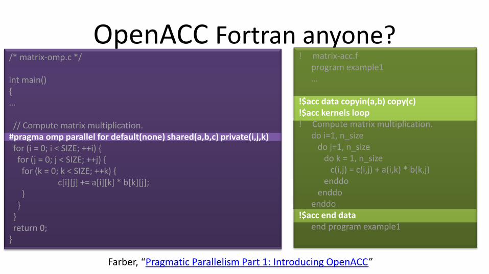
OpenACC Fortran anyone?
Farber, “Pragmatic Parallelism Part 1: Introducing OpenACC”
! matrix-acc.f program example1 … !$acc data copyin(a,b) copy(c) !$acc kernels loop ! Compute matrix multiplication. do i=1, n_size do j=1, n_size do k = 1, n_size c(i,j) = c(i,j) + a(i,k) * b(k,j) enddo enddo enddo !$acc end data end program example1
/* matrix-omp.c */ int main() { … // Compute matrix multiplication. #pragma omp parallel for default(none) shared(a,b,c) private(i,j,k) for (i = 0; i < SIZE; ++i) { for (j = 0; j < SIZE; ++j) { for (k = 0; k < SIZE; ++k) { c[i][j] += a[i][k] * b[k][j]; } } } return 0; }
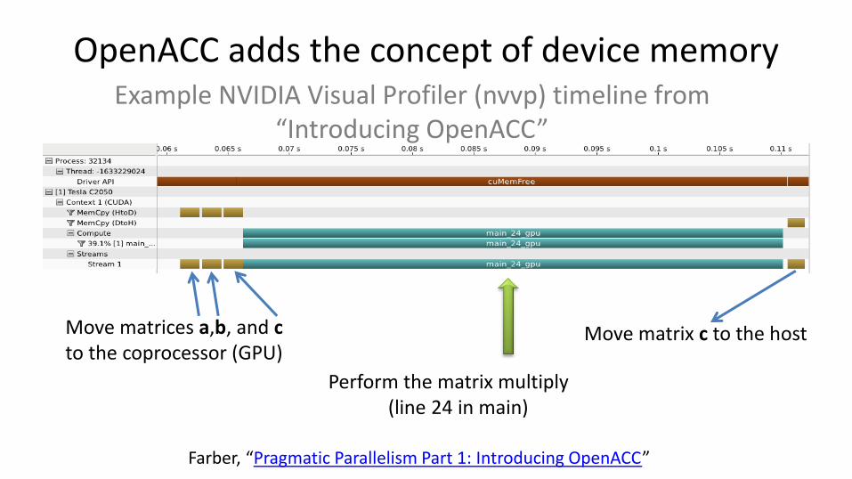
OpenACC adds the concept of device memory
Move matrices a,b, and c to the coprocessor (GPU)
Move matrix c to the host
Perform the matrix multiply (line 24 in main)
Example NVIDIA Visual Profiler (nvvp) timeline from “Introducing OpenACC”
Farber, “Pragmatic Parallelism Part 1: Introducing OpenACC”
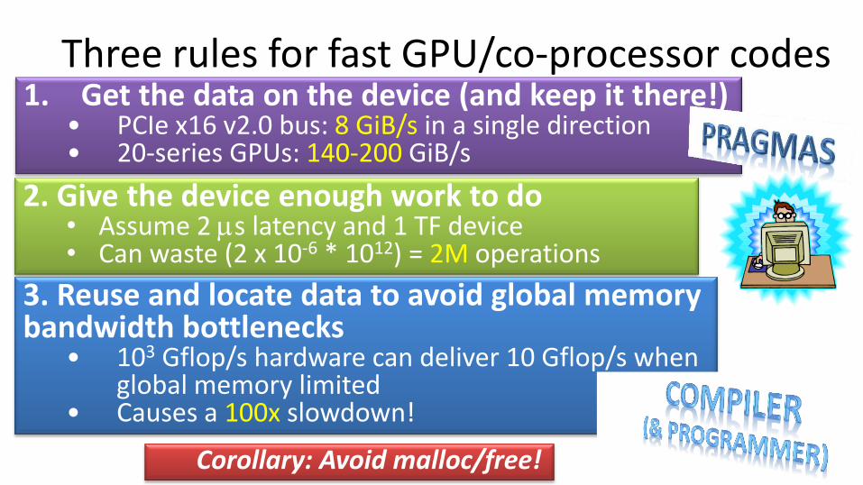
Three rules for fast GPU/co-processor codes 1. Get the data on the device (and keep it there!)
• PCIe x16 v2.0 bus: 8 GiB/s in a single direction • 20-series GPUs: 140-200 GiB/s
2. Give the device enough work to do • Assume 2 ms latency and 1 TF device • Can waste (2 x 10-6 * 1012) = 2M operations
3. Reuse and locate data to avoid global memory bandwidth bottlenecks
• 103 Gflop/s hardware can deliver 10 Gflop/s when global memory limited
• Causes a 100x slowdown!
Corollary: Avoid malloc/free!
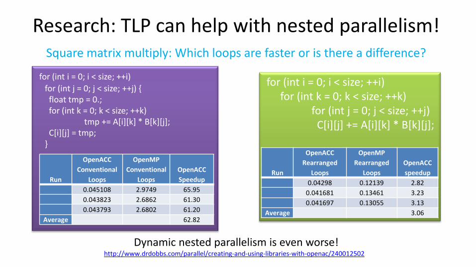
Research: TLP can help with nested parallelism!
for (int i = 0; i < size; ++i) for (int k = 0; k < size; ++k) for (int j = 0; j < size; ++j) C[i][j] += A[i][k] * B[k][j];
for (int i = 0; i < size; ++i)
for (int j = 0; j < size; ++j) { float tmp = 0.; for (int k = 0; k < size; ++k) tmp += A[i][k] * B[k][j]; C[i][j] = tmp; }
Run
OpenACC
Rearranged
Loops
OpenMP
Rearranged
Loops
OpenACC
speedup
0.04298 0.12139 2.82
0.041681 0.13461 3.23
0.041697 0.13055 3.13
Average 3.06
Run
OpenACC
Conventional
Loops
OpenMP
Conventional
Loops
OpenACC
Speedup
0.045108 2.9749 65.95
0.043823 2.6862 61.30
0.043793 2.6802 61.20
Average 62.82
Square matrix multiply: Which loops are faster or is there a difference?
Dynamic nested parallelism is even worse! http://www.drdobbs.com/parallel/creating-and-using-libraries-with-openac/240012502
DATA
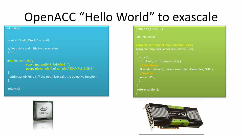
OpenACC “Hello World” to exascale double objFunc( ... ) { double err=0.; #pragma acc parallel loop reduction(+:err) #pragma omp parallel for reduction(+ : err) { err = 0.; for(int i=0; i < nExamples; i++) { // transform float d=myFunc(i, param, example, nExamples, NULL); //reduce err += d*d; } } return sqrt(err); }
int main() { cout << "Hello World" << endl; // load data and initialize parameters init(); #pragma acc data \ copyin(param[0:N_PARAM-1]) \ pcopyin(example[0:nExamples*EXAMPLE_SIZE-1]) { optimize( objFunc ); // the optimizer calls the objective function } return 0; }
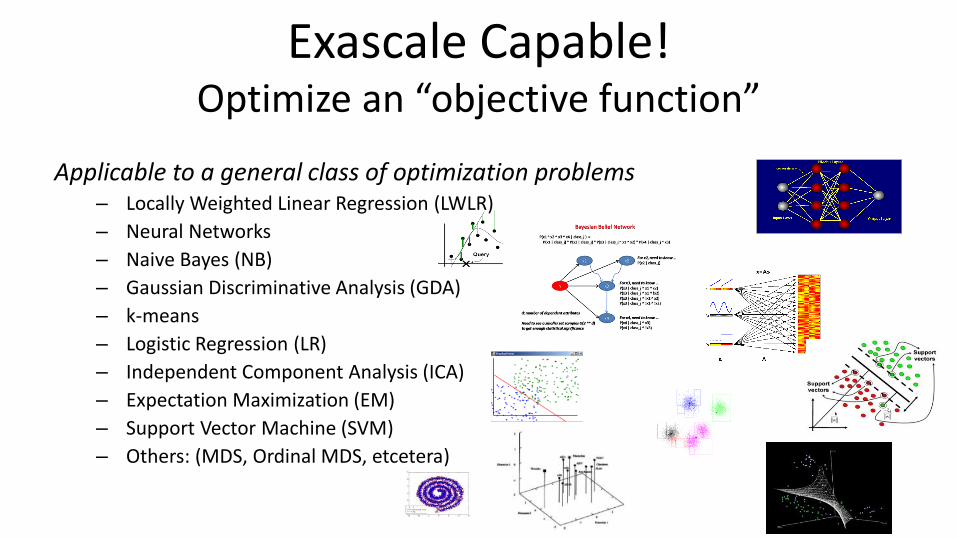
Applicable to a general class of optimization problems – Locally Weighted Linear Regression (LWLR)
– Neural Networks
– Naive Bayes (NB)
– Gaussian Discriminative Analysis (GDA)
– k-means
– Logistic Regression (LR)
– Independent Component Analysis (ICA)
– Expectation Maximization (EM)
– Support Vector Machine (SVM)
– Others: (MDS, Ordinal MDS, etcetera)
Exascale Capable! Optimize an “objective function”
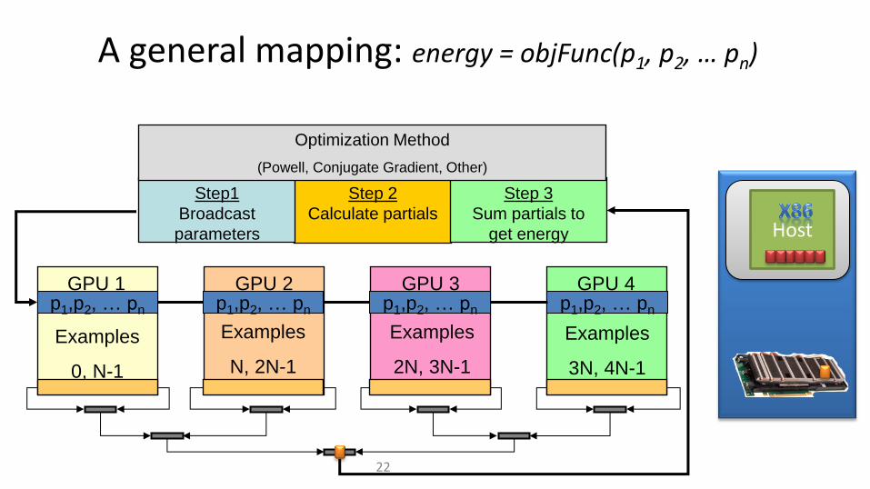
A general mapping: energy = objFunc(p1, p2, … pn)
22
Examples
0, N-1
Examples
N, 2N-1
Examples
2N, 3N-1
Examples
3N, 4N-1
Step 2
Calculate partials
Step 3
Sum partials to
get energy
Step1
Broadcast
parameters
Optimization Method
(Powell, Conjugate Gradient, Other)
GPU 1 GPU 2 GPU 3 p1,p2, … pn p1,p2, … pn p1,p2, … pn p1,p2, … pn
GPU 4
Host
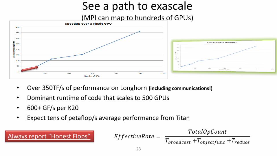
See a path to exascale (MPI can map to hundreds of GPUs)
23
• Over 350TF/s of performance on Longhorn (including communications!)
• Dominant runtime of code that scales to 500 GPUs
• 600+ GF/s per K20
• Expect tens of petaflop/s average performance from Titan
𝐸𝑓𝑓𝑒𝑐𝑡𝑖𝑣𝑒𝑅𝑎𝑡𝑒 = 𝑇𝑜𝑡𝑎𝑙𝑂𝑝𝐶𝑜𝑢𝑛𝑡
𝑇𝑏𝑟𝑜𝑎𝑑𝑐𝑎𝑠𝑡 +𝑇𝑜𝑏𝑗𝑒𝑐𝑡𝑓𝑢𝑛𝑐 +𝑇𝑟𝑒𝑑𝑢𝑐𝑒 Always report “Honest Flops”
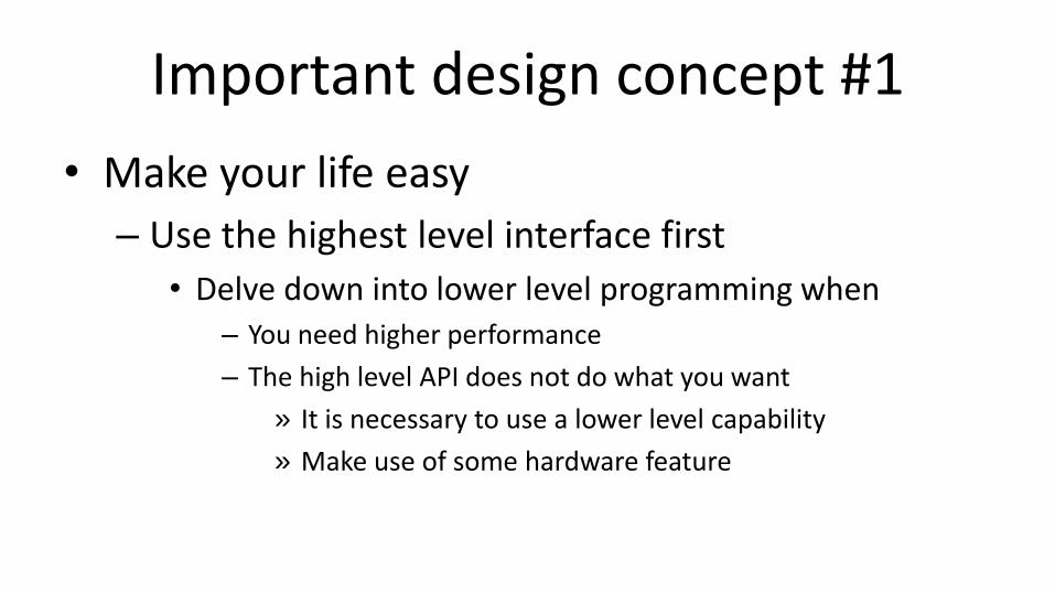
Important design concept #1
• Make your life easy
– Use the highest level interface first
• Delve down into lower level programming when – You need higher performance
– The high level API does not do what you want
» It is necessary to use a lower level capability
» Make use of some hardware feature
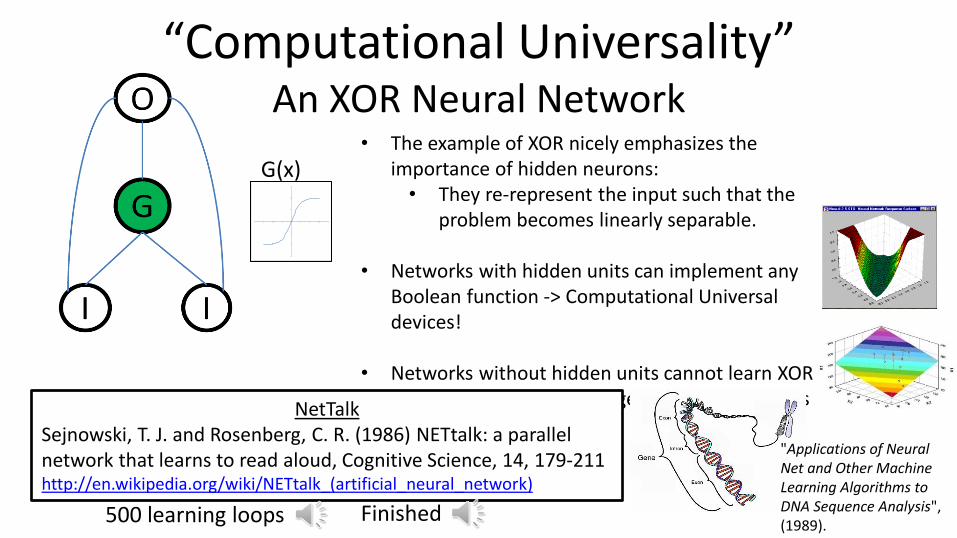
“Computational Universality” An XOR Neural Network
• The example of XOR nicely emphasizes the importance of hidden neurons:
• They re-represent the input such that the problem becomes linearly separable.
• Networks with hidden units can implement any Boolean function -> Computational Universal devices!
• Networks without hidden units cannot learn XOR • Cannot represent large classes of problems
G(x)
NetTalk Sejnowski, T. J. and Rosenberg, C. R. (1986) NETtalk: a parallel network that learns to read aloud, Cognitive Science, 14, 179-211 http://en.wikipedia.org/wiki/NETtalk_(artificial_neural_network)
500 learning loops Finished
"Applications of Neural Net and Other Machine Learning Algorithms to DNA Sequence Analysis", (1989).
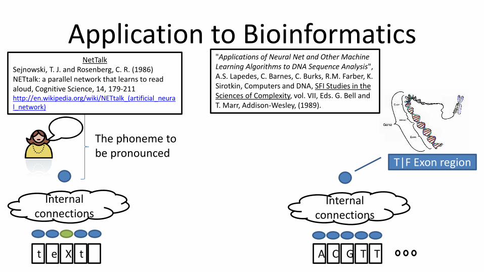
Application to Bioinformatics
Internal connections
The phoneme to be pronounced
NetTalk Sejnowski, T. J. and Rosenberg, C. R. (1986) NETtalk: a parallel network that learns to read aloud, Cognitive Science, 14, 179-211 http://en.wikipedia.org/wiki/NETtalk_(artificial_neural_network)
Internal connections
t t e X A T C G T
"Applications of Neural Net and Other Machine Learning Algorithms to DNA Sequence Analysis", A.S. Lapedes, C. Barnes, C. Burks, R.M. Farber, K. Sirotkin, Computers and DNA, SFI Studies in the Sciences of Complexity, vol. VII, Eds. G. Bell and T. Marr, Addison-Wesley, (1989).
T|F Exon region
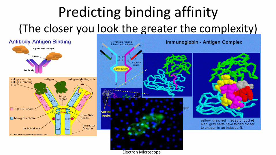
Predicting binding affinity (The closer you look the greater the complexity)
Electron Microscope
The question for computational biology
• How do we know you are not playing expensive computer games with our money?
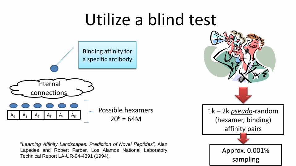
Utilize a blind test
Internal connections
A0
Binding affinity for a specific antibody
A1 A2 A3 A4 A5
Possible hexamers 206 = 64M
1k – 2k pseudo-random (hexamer, binding)
affinity pairs
Approx. 0.001% sampling
“Learning Affinity Landscapes: Prediction of Novel Peptides”, Alan
Lapedes and Robert Farber, Los Alamos National Laboratory
Technical Report LA-UR-94-4391 (1994).
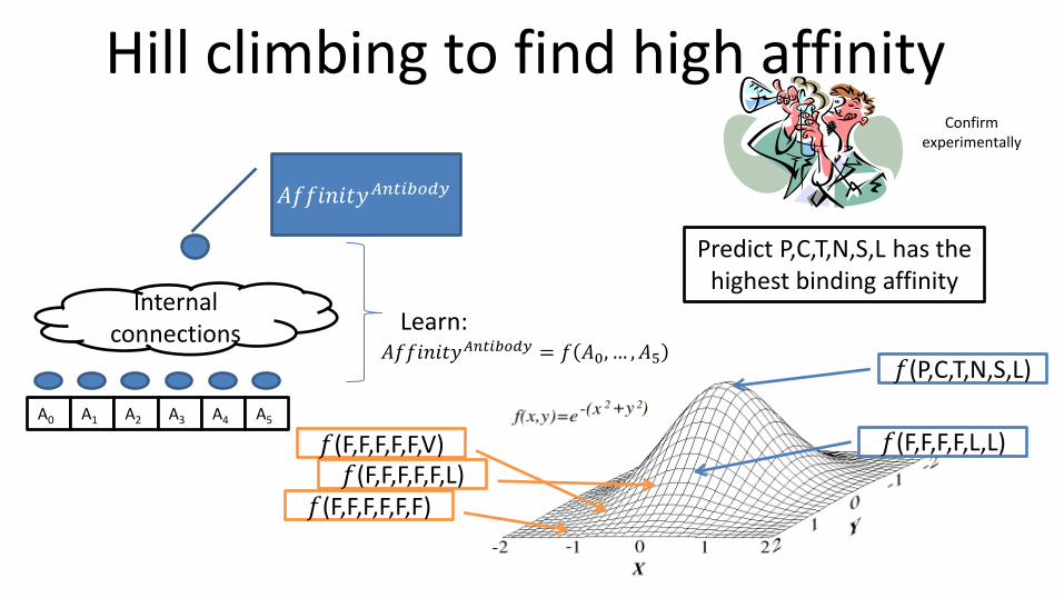
Hill climbing to find high affinity
Internal connections
A0
𝐴𝑓𝑓𝑖𝑛𝑖𝑡𝑦𝐴𝑛𝑡𝑖𝑏𝑜𝑑𝑦
A1 A2 A3 A4 A5
Learn: 𝐴𝑓𝑓𝑖𝑛𝑖𝑡𝑦𝐴𝑛𝑡𝑖𝑏𝑜𝑑𝑦 = 𝑓 𝐴0, … , 𝐴5
𝑓(F,F,F,F,F,F) 𝑓(F,F,F,F,F,L)
𝑓(F,F,F,F,F,V) 𝑓(F,F,F,F,L,L)
𝑓(P,C,T,N,S,L)
Predict P,C,T,N,S,L has the highest binding affinity
Confirm experimentally
Two important points
• The computer appears to correctly predict experimental data
• Demonstrated that complex binding affinity relationships can be learned from a small set of samples – Necessary because it is only possible to sample a very
small subset of the binding affinity landscape for drug candidates
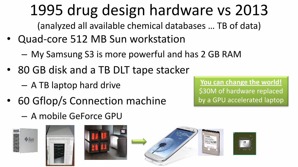
1995 drug design hardware vs 2013 (analyzed all available chemical databases … TB of data)
• Quad-core 512 MB Sun workstation
– My Samsung S3 is more powerful and has 2 GB RAM
• 80 GB disk and a TB DLT tape stacker
– A TB laptop hard drive
• 60 Gflop/s Connection machine
– A mobile GeForce GPU
You can change the world! $30M of hardware replaced by a GPU accelerated laptop
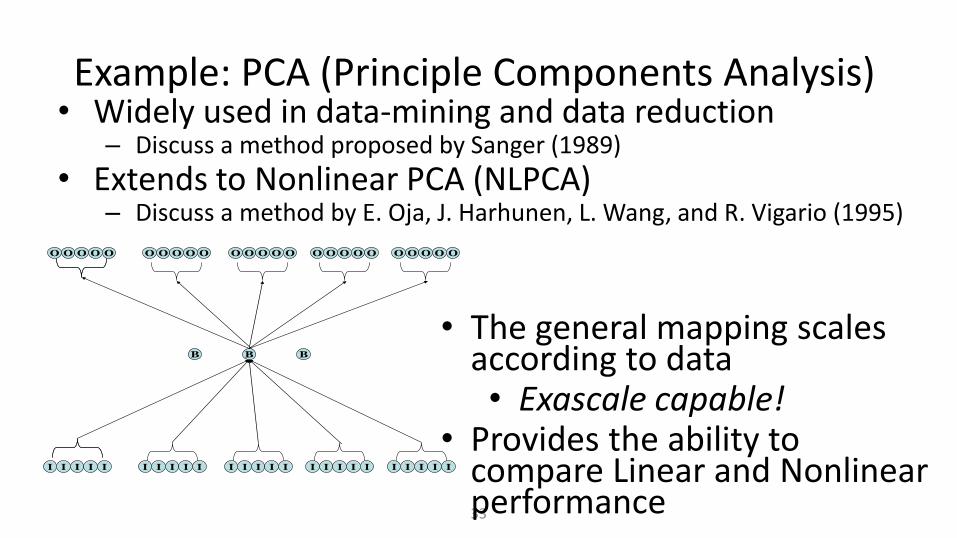
Example: PCA (Principle Components Analysis) • Widely used in data-mining and data reduction
– Discuss a method proposed by Sanger (1989)
• Extends to Nonlinear PCA (NLPCA) – Discuss a method by E. Oja, J. Harhunen, L. Wang, and R. Vigario (1995)
33
B B B
O O O OO O O O OO O O O OO O O O OOO O O OO
I I I II I I I II I I I II I I I III I I II
• The general mapping scales according to data • Exascale capable!
• Provides the ability to compare Linear and Nonlinear performance
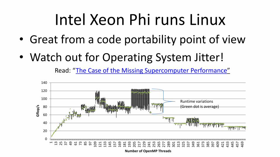
Intel Xeon Phi runs Linux • Great from a code portability point of view
• Watch out for Operating System Jitter! Read: “The Case of the Missing Supercomputer Performance”
0
20
40
60
80
100
120
140
1
13
25
37
49
61
73
85
97
10
9
12
1
13
3
14
5
15
7
16
9
18
1
19
3
20
5
21
7
22
9
24
1
25
3
26
5
27
7
28
9
30
1
31
3
32
5
33
7
34
9
36
1
37
3
38
5
39
7
40
9
42
1
43
3
44
5
45
7
46
9
Gfl
op
/s
Number of OpenMP Threads
Runtime variations (Green dot is average)
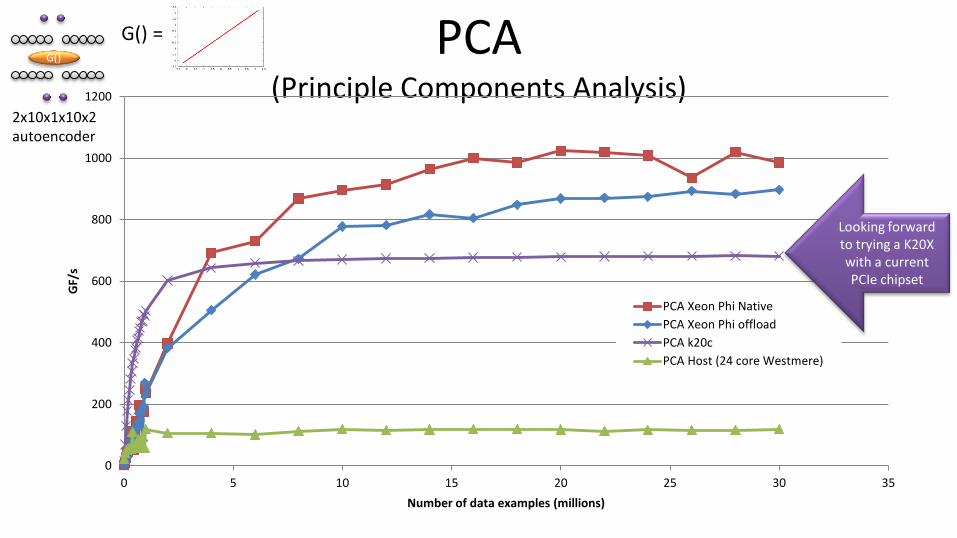
PCA (Principle Components Analysis)
0
200
400
600
800
1000
1200
0 5 10 15 20 25 30 35
GF/
s
Number of data examples (millions)
PCA Xeon Phi Native
PCA Xeon Phi offload
PCA k20c
PCA Host (24 core Westmere)
G()
2x10x1x10x2 autoencoder
G() =
Looking forward to trying a K20X with a current PCIe chipset
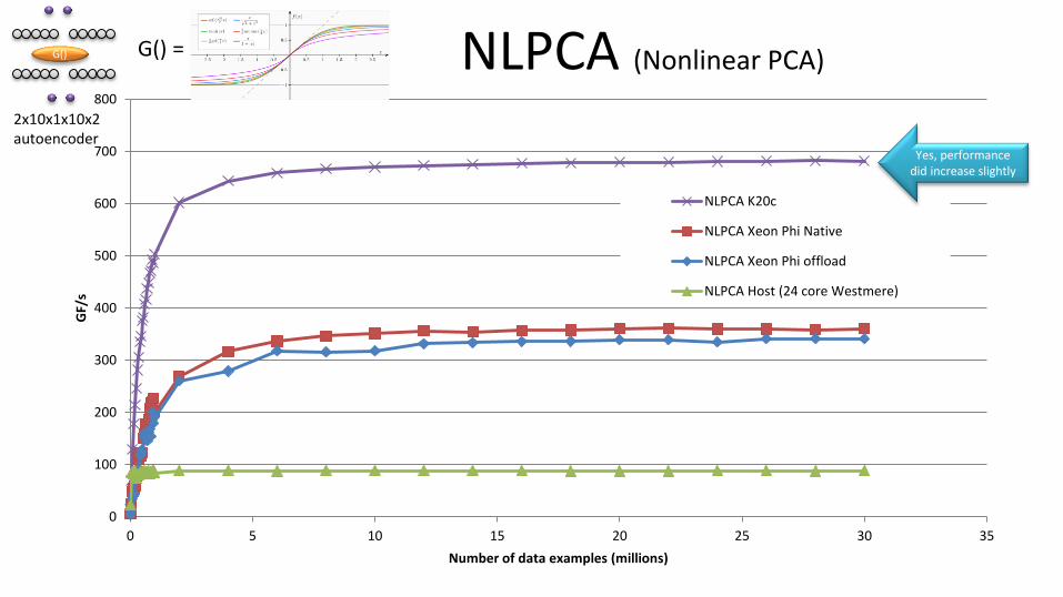
NLPCA (Nonlinear PCA)
0
100
200
300
400
500
600
700
800
0 5 10 15 20 25 30 35
GF/
s
Number of data examples (millions)
NLPCA K20c
NLPCA Xeon Phi Native
NLPCA Xeon Phi offload
NLPCA Host (24 core Westmere)
G() = G()
2x10x1x10x2 autoencoder
Yes, performance did increase slightly
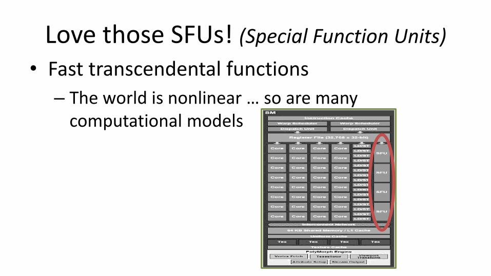
Love those SFUs! (Special Function Units)
• Fast transcendental functions
– The world is nonlinear … so are many computational models
TF/s devices open the door to new topics
• Works great for manufacturing optimization – Best product for lowest cost of materials – Works great for color matching
• Multiterm objective functions – Best design for the lowest (cost, weight, {your metric here}, …) – A teraflop/s per device can run many optimizations to map the
decision space.
• Machine learning with memory or variable inputs – Recurrent neural networks, IIR filters, …. – Have to iterate the network during training
You can change the world!
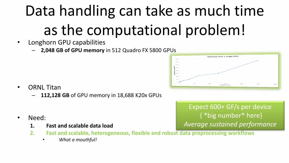
Data handling can take as much time as the computational problem!
• Longhorn GPU capabilities – 2,048 GB of GPU memory in 512 Quadro FX 5800 GPUs
• ORNL Titan – 112,128 GB of GPU memory in 18,688 K20x GPUs
• Need: 1. Fast and scalable data load 2. Fast and scalable, heterogeneous, flexible and robust data preprocessing workflows
• What a mouthful!
Expect 600+ GF/s per device { *big number* here}
Average sustained performance
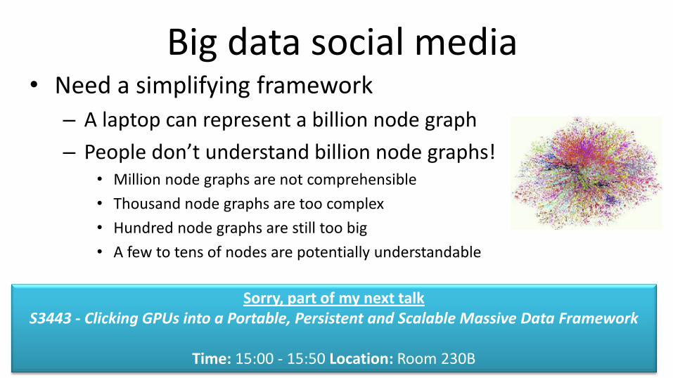
Big data social media • Need a simplifying framework
– A laptop can represent a billion node graph
– People don’t understand billion node graphs! • Million node graphs are not comprehensible
• Thousand node graphs are too complex
• Hundred node graphs are still too big
• A few to tens of nodes are potentially understandable
Validate against 3rd party experts and machine metrics • Understand this is a lens looking into a social reality • Cannot forget that the computer only represents reality!
Sorry, part of my next talk S3443 - Clicking GPUs into a Portable, Persistent and Scalable Massive Data Framework
Time: 15:00 - 15:50 Location: Room 230B
Important design concept #2
• Try to maintain just one source tree – OpenACC/OpenMP pragmas are interesting
(disclaimer/shameless commerce:
I’m writing an OpenACC book)
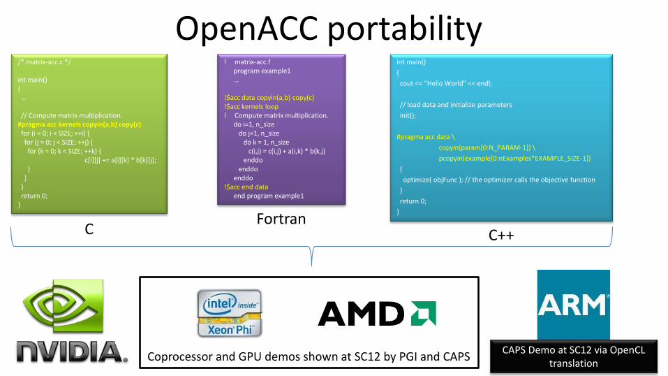
OpenACC portability /* matrix-acc.c */ int main() { … // Compute matrix multiplication. #pragma acc kernels copyin(a,b) copy(c) for (i = 0; i < SIZE; ++i) { for (j = 0; j < SIZE; ++j) { for (k = 0; k < SIZE; ++k) { c[i][j] += a[i][k] * b[k][j]; } } } return 0; }
! matrix-acc.f program example1 … !$acc data copyin(a,b) copy(c) !$acc kernels loop ! Compute matrix multiplication. do i=1, n_size do j=1, n_size do k = 1, n_size c(i,j) = c(i,j) + a(i,k) * b(k,j) enddo enddo enddo !$acc end data end program example1
int main()
{
cout << "Hello World" << endl;
// load data and initialize parameters
init();
#pragma acc data \
copyin(param[0:N_PARAM-1]) \
pcopyin(example[0:nExamples*EXAMPLE_SIZE-1])
{
optimize( objFunc ); // the optimizer calls the objective function
}
return 0;
}
C Fortran
C++
Coprocessor and GPU demos shown at SC12 by PGI and CAPS CAPS Demo at SC12 via OpenCL
translation
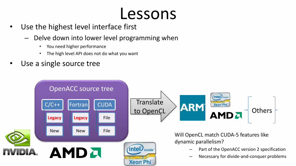
Lessons • Use the highest level interface first
– Delve down into lower level programming when • You need higher performance
• The high level API does not do what you want
• Use a single source tree
OpenACC source tree
C/C++
Legacy
New
Fortran
Legacy
New
CUDA
File
File
Translate to OpenCL
Will OpenCL match CUDA-5 features like dynamic parallelism?
– Part of the OpenACC version 2 specification
– Necessary for divide-and-conquer problems
Others
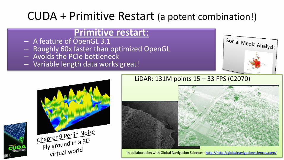
CUDA + Primitive Restart (a potent combination!)
Primitive restart: – A feature of OpenGL 3.1 – Roughly 60x faster than optimized OpenGL – Avoids the PCIe bottleneck – Variable length data works great!
44
LiDAR: 131M points 15 – 33 FPS (C2070)
In collaboration with Global Navigation Sciences (http://http://globalnavigationsciences.com/
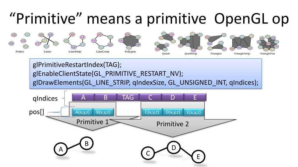
“Primitive” means a primitive OpenGL op
glPrimitiveRestartIndex(TAG); glEnableClientState(GL_PRIMITIVE_RESTART_NV); glDrawElements(GL_LINE_STRIP, qIndexSize, GL_UNSIGNED_INT, qIndices);
A B TAG C D E qIndices
Primitive 1
A(x,y,z) B(x,y,z)
A B
Primitive 2
C(x,y,z) D(x,y,z) E(x,y,z)
C D
E
pos[]
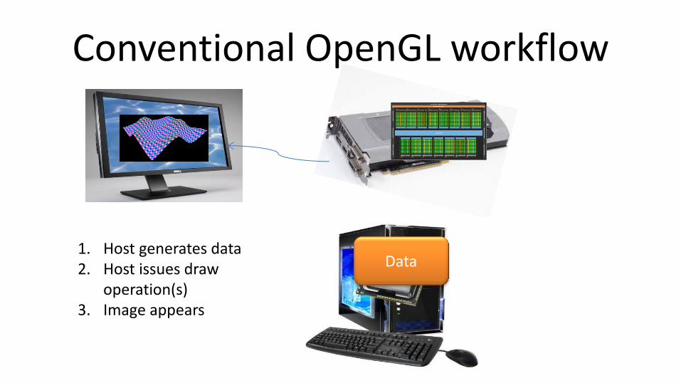
Conventional OpenGL workflow
Data 1. Host generates data 2. Host issues draw
operation(s) 3. Image appears
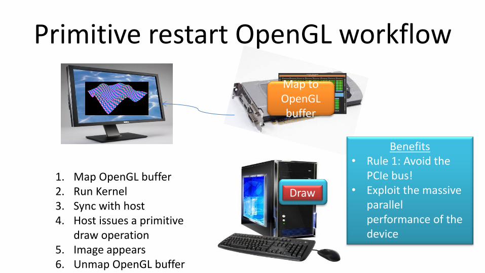
Primitive restart OpenGL workflow
Map to OpenGL buffer
1. Map OpenGL buffer 2. Run Kernel 3. Sync with host 4. Host issues a primitive
draw operation 5. Image appears 6. Unmap OpenGL buffer
Kernel Draw
Benefits • Rule 1: Avoid the
PCIe bus! • Exploit the massive
parallel performance of the device
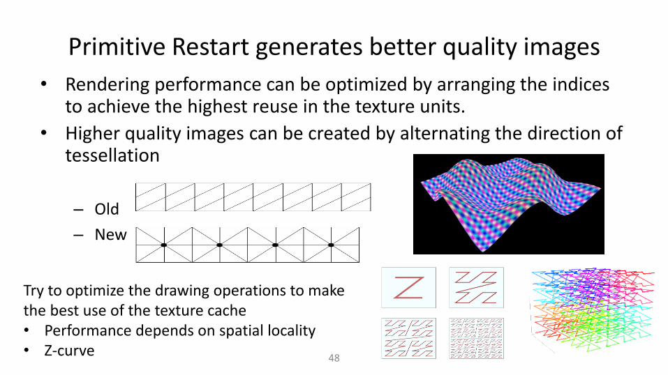
Primitive Restart generates better quality images
• Rendering performance can be optimized by arranging the indices to achieve the highest reuse in the texture units.
• Higher quality images can be created by alternating the direction of tessellation
– Old
– New
48
Try to optimize the drawing operations to make the best use of the texture cache • Performance depends on spatial locality • Z-curve
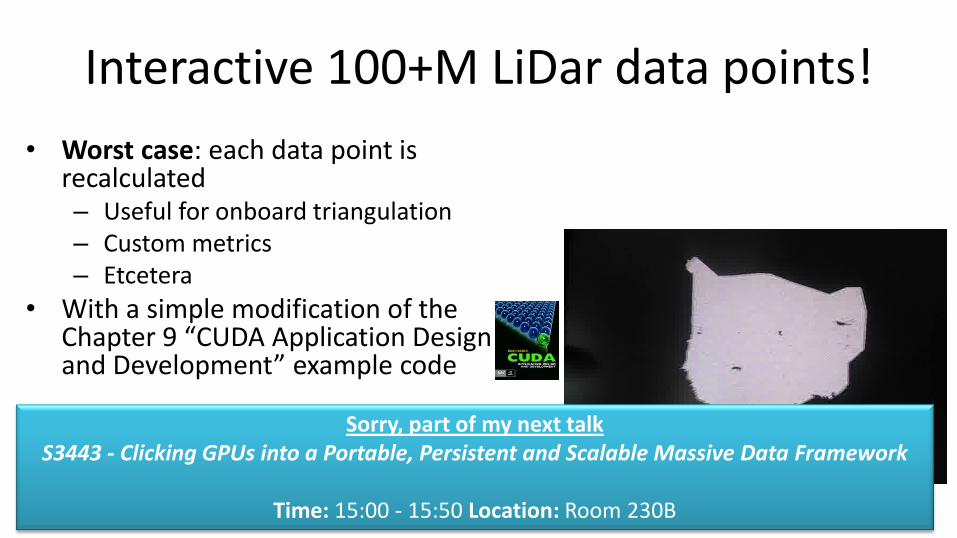
Interactive 100+M LiDar data points!
• Worst case: each data point is recalculated – Useful for onboard triangulation – Custom metrics – Etcetera
• With a simple modification of the Chapter 9 “CUDA Application Design and Development” example code
Sorry, part of my next talk S3443 - Clicking GPUs into a Portable, Persistent and Scalable Massive Data Framework
Time: 15:00 - 15:50 Location: Room 230B

Sedláček, M. (2004). Evaluation of RGB and HSV Models in Human Faces Detection. Central European Seminar on Computer Graphics, Budmerice. CompSysTech’2004 , (pp. 125-131).
The entire segmentation method __global__ void kernelSkin(float4* pos, uchar4 *colorPos, unsigned int width, unsigned int height, int lowPureG, int highPureG, int lowPureR, int highPureR) { unsigned int x = blockIdx.x*blockDim.x + threadIdx.x; unsigned int y = blockIdx.y*blockDim.y + threadIdx.y; int r = colorPos[y*width+x].x; int g = colorPos[y*width+x].y; int b = colorPos[y*width+x].z; int pureR = 255*( ((float)r)/(r+g+b)); int pureG = 255*( ((float)g)/(r+g+b)); if( !( (pureG > lowPureG) && (pureG < highPureG) && (pureR > lowPureR) && (pureR < highPureR) ) ) colorPos[y*width+x] = make_uchar4(0,0,0,0); }
For the demo, think Kinect and 3D morphing for augmented reality (identify flesh colored blobs for hands)
Artifacts caused by picking a colorspace rectangle rather than an ellipse
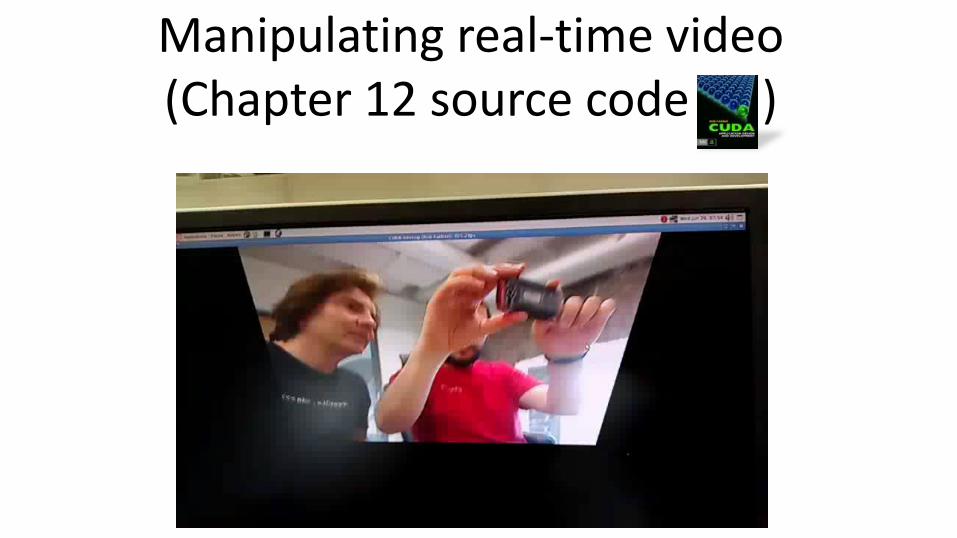
Manipulating real-time video (Chapter 12 source code )
Thank you! Rob Farber
Chief Scientist, BlackDog Endeavors, LLC Author, “CUDA Application Design and Development”
Research consultant: ICHEC, Fortune 100 companies, and others Scientist: .
Dr. Dobb’s Journal CUDA & OpenACC tutorials
• OpenCL “The Code Project” tutorials
• Columnist Scientific Computing, and other venues