S2N2: A FPGA Accelerator for Streaming Spiking NeuralNetworks

Alireza Khodamoradialirezak@eng.ucsd.edu

University of California, San Diego

Kristof Denolfkristof@xilinx.com

Xilinx

Ryan Kastnerkastner@eng.ucsd.edu

University of California, San Diego

ABSTRACTSpiking Neural Networks (SNNs) are the next generation of Artifi-cial Neural Networks (ANNs) that utilize an event-based represen-tation to perform more efficient computation. Most SNN implemen-tations have a systolic array-based architecture and, by assuminghigh sparsity in spikes, significantly reduce computing in theirdesigns. This work shows this assumption does not hold for ap-plications with signals of large temporal dimension. We develop astreaming SNN (S2N2) architecture that can support fixed-per-layeraxonal and synaptic delays for its network. Our architecture is builtupon FINN and thus efficiently utilizes FPGA resources. We showhow radio frequency processing matches our S2N2 computationalmodel. By not performing tick-batching, a stream of RF samples canefficiently be processed by S2N2, improving the memory utilizationby more than three orders of magnitude.

CCS CONCEPTS• Hardware → Hardware accelerators; High-speed input / out-put; Reconfigurable logic applications; Emerging architectures.

KEYWORDSSpiking Neural Networks, Streaming, FINN, RF

ACM Reference Format:Alireza Khodamoradi, Kristof Denolf, and Ryan Kastner. 2021. S2N2: AFPGA Accelerator for Streaming Spiking Neural Networks. In Proceedingsof the 2021 ACM/SIGDA International Symposium on Field ProgrammableGate Arrays (FPGA ’21), February 28-March 2, 2021, Virtual Event, USA. ACM,New York, NY, USA, 12 pages. https://doi.org/10.1145/3431920.3439283

1 INTRODUCTIONArtificial Neural Networks have shown remarkable success in large-scale image and video recognition [39, 41], speech recognition[5, 13], radio signal classification [33], and many other applicationdomains [15, 20]. Spiking Neural Networks (SNNs) use an event-based model that better mimics biological neurons [12, 25] with thegoal of providing high prediction accuracy while using minimalenergy [42]. Recent advancements in SNN architecture design andtraining methods show promise in matching the accuracy of non-spiking ANNs [2, 3, 10, 40] and the potential to out-perform a

Permission to make digital or hard copies of all or part of this work for personal orclassroom use is granted without fee provided that copies are not made or distributedfor profit or commercial advantage and that copies bear this notice and the full citationon the first page. Copyrights for components of this work owned by others than ACMmust be honored. Abstracting with credit is permitted. To copy otherwise, or republish,to post on servers or to redistribute to lists, requires prior specific permission and/or afee. Request permissions from permissions@acm.org.FPGA ’21, February 28-March 2, 2021, Virtual Event, USA© 2021 Association for Computing Machinery.ACM ISBN 978-1-4503-8218-2/21/02. . . $15.00https://doi.org/10.1145/3431920.3439283

similar-sized non-spiking ANN [8]. However, much work remainsuntil we fully uncover the potentials of SNNs [42].

A conventional neuron model assumes every input requirescalculation and performs 𝑁 operations, e.g., multiplying and ac-cumulating 𝑁 input values with 𝑁 weights (and an optional bias -see Equation 1). A typical convolutional layer in a modern feedfor-ward neural network includes many neurons with an equal numberof inputs (fan-in). This architecture creates patterns suitable formassively parallel implementations. Frameworks such as FINN [4],fpgaConvNet [48], and Eyeriss [6] provide efficient implementa-tions of this architecture on FPGAs.

Conversely, event-based neural networks reduce wasted com-putation by only processing received events. For example whenan event-based neuron with fan-in=𝑁 receives𝑀 < 𝑁 events, cal-culating the input only requires 𝑀 operations (Equation 2). Thisassumes a certain amount of sparsity and requires dynamic han-dling of events. This sparsity creates a run-time dependency basedon the input data and induces unpredictable and potentially irreg-ular memory accesses. Therefore exploiting parallelism in SNN ismore challenging than CNNs, DNNs, and other more traditionalneural networks.

Previous works such as IBM TrueNorth [2], Intel Loihi [9], SpiN-Naker [35], and BlueHive [28] have shown that processing SNNevents can be efficiently implemented in custom hardware for bothtraining and inference. Neurogrid [3] uses a mixed analog-digital ap-proach for simulating large-scale spiking models and Minitaur [31]and SpinalFlow [30] describe inference accelerators for SNNs. Eventprocessing is either done by encoding and storing events in a bufferto be processed in a systolic fashion (tick-batching) [2, 9, 30, 31] ora spike-routing mechanism is used to prevent deadlocks [3, 28, 35].

In this work, we introduce a streaming accelerator for spikingneural networks, S2N2. Our design efficiently supports both ax-onal and synaptic delays for feedforward networks with interlayerconnections. We show that because of the spikes’ binary nature, abinary tensor can be used for addressing the input events of a layer.We describe the condition when addressing events with a binarytensor, and no tick-batching (streaming) can provide a better mem-ory utilization compared to encoding events and tick-batching. Weshow that this condition depends on the input’s sparsity (more de-tail in Section 3.3) and holds, for example, applications, in particularfor Radio Frequency (RF) applications.

We use the FINN framework [47] as our baseline and extend itwith new functions for supporting our event-based processing ofSNNs. Our proposed changes can maintain the high throughput ofFINN and provide an efficient streaming implementation for SNNsby benefiting from FINN’s optimized utilization footprint.

We also propose novel example applications for SNNs in theRF domain that can benefit from S2N2’s streaming architecture.

Session 3: Machine Learning and Supporting Algorithms FPGA ’21, February 28–March 2, 2021, Virtual Event, USA

194

By looking at RF samples as events in In-phase and Quadrature(I/Q) plane, RF samples can be turned into highly sparse events asinput to a SNN. RF inputs available in RF datasets [32, 34] have alarge temporal dimension, and a SNN designed for classifying theseinputs can efficiently be implemented in S2N2.

In addition, our design is tested by using some of the publishedapplications for SNNs in the image classification domain [18, 40].In order to adopt these previously published spiking networks toS2N2, we propose new architectural changes in these networksand show that modified networks can maintain their accuracy afterre-training with new hyperparameters.

Our contributions can be summarized as following:• We introduce a new streaming architecture, S2N2, for accel-erating SNNs on FPGA platforms.

• We describe how to reduce the memory utilization for inputswith a large temporal dimension.

• We propose novel applications for SNNs in the RF domainthat can benefit from our streaming architecture.

• We release our code as open-sourced to enhance accessibilityand aid in future comparisons of our work 1.

The remainder of the paper is organized as follows. In Section 2,we introduce SNNs in more depth and review the previous work onSNN FPGA implementations. S2N2 is described in detail in Section 3and we demonstrate its advantages and implementation results forRF applications in Section 4. Additionally, Section 5 applies the S2N2architecture to previously published SNNs for image classifications.We conclude our work in section 6.

2 SPIKING NEURAL NETWORKSpiking neural networks are the third generation of ANNs devel-oped to process information more similar to biological neural net-works [25, 42]. In these networks, neurons propagate informationby using spikes. The information is coded into the rate and time-of-arrival of the spikes.

Figure 1 shows an example comparison between a frame-basedinput and an event-based input with rate-coded spikes. In general,input to each layer in a non-spiking neural network is a tensorof values (a multi-channel matrix). In contrast, in a SNN, inputsto each layer are events that have temporal and spatial positions.The temporal dimension of the input in SNNs consists of several"ticks". A tick is the minimum unit of time in a SNN that a neuronevaluates its input, updates its potential, and, depending on itsmodel parameters, may generate a spike in its output.

For a more clear comparison, we look at the operations requiredfor evaluating inputs in non-spiking and spiking neurons. Input toa non-spiking neuron is calculated as follows:

𝐼 =

𝑁∑𝑖=0

𝑤𝑖𝑥𝑖 (1)

Here, 𝑥𝑖 are the input values and𝑤𝑖 are their associated weightsand bias is not shown.

While input to a spiking neuron at tick=𝑡 is calculated as follow-ing:

1github.com/arkhodamoradi/s2n2

𝐼𝑡 =∑𝑖∈𝑆𝑡

𝑤𝑖 (2)

Here, 𝑆𝑡 is the set of inputs to the neuron that have a spike attick=𝑡 , and𝑤𝑖 are the weights associated with those inputs.

Figure 1: A frame-based input (on the left) is a matrix ofnumbers. An event-based input (on the right) includes trainsof spikes. In this example, the number of trains is equal tothe number of pixels in the frame. The duration of the spiketrains is equal to the number of ticks. At each tick, up to onespike can exist in each train.

With sparsity in input spikes, Equation 2 requires fewer andsimpler accumulation operations compared to the fixed number ofMAC operations required in Equation 1. However, Equation 1 ismore suitable for applying techniques such as loop-unrolling forexploiting parallelism. In addition, Equation 2 requires memory tostore 𝑆 to keep track of input spikes. Later in this work, we providesolutions to efficiently implement Equation 2 on custom hardware.

In a conventional ANN, an activation function of a neuron de-fines the output of that neuron given an input. In SNNs, neuron’soutput and evaluation of neuron potential are governed by neuron’smodel.

Neuron models used in SNNs are biologically plausible modelsthat are computationally more powerful units compared to activa-tion functions used in non-spiking networks [12]. These modelsare capable of extracting the temporal information embedded intheir input and perform more complex tasks [25].

Although more complex mathematical models such as Izhike-vich [16] and Hodgkin–Huxley [14] can accurately model a biolog-ical neuron’s behavior, current training methods for SNNs are notgeared to train these complex models [42]. For now, simpler modelssuch as Integrate and Fire (IF) and Leaky Integrate and Fire (LIF)are more prevalent in current SNN applications. In this work, weuse a LIF model with one internal parameter.

2.1 LIF ModelLeaky Integrate and Fire (LIF) model is a neuron model widely usedin SNN applications [18, 21, 36, 40, 50]. LIF model memorizes itspast inputs by adding every input to its membrane potential anduses a leak (decay) parameter to forget them. This leak parameter isreflecting the diffusion of ions that occurs through the membranewhen some equilibrium is not reached in the cell:

Session 3: Machine Learning and Supporting Algorithms FPGA ’21, February 28–March 2, 2021, Virtual Event, USA

195

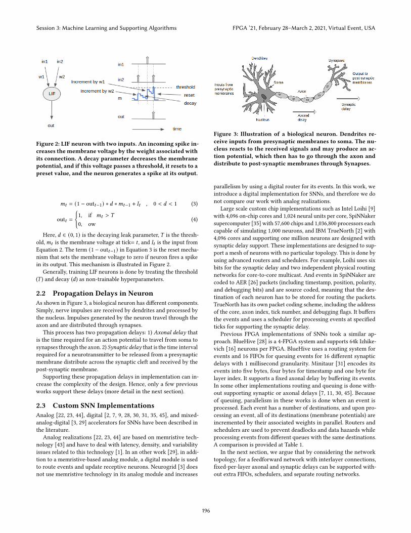
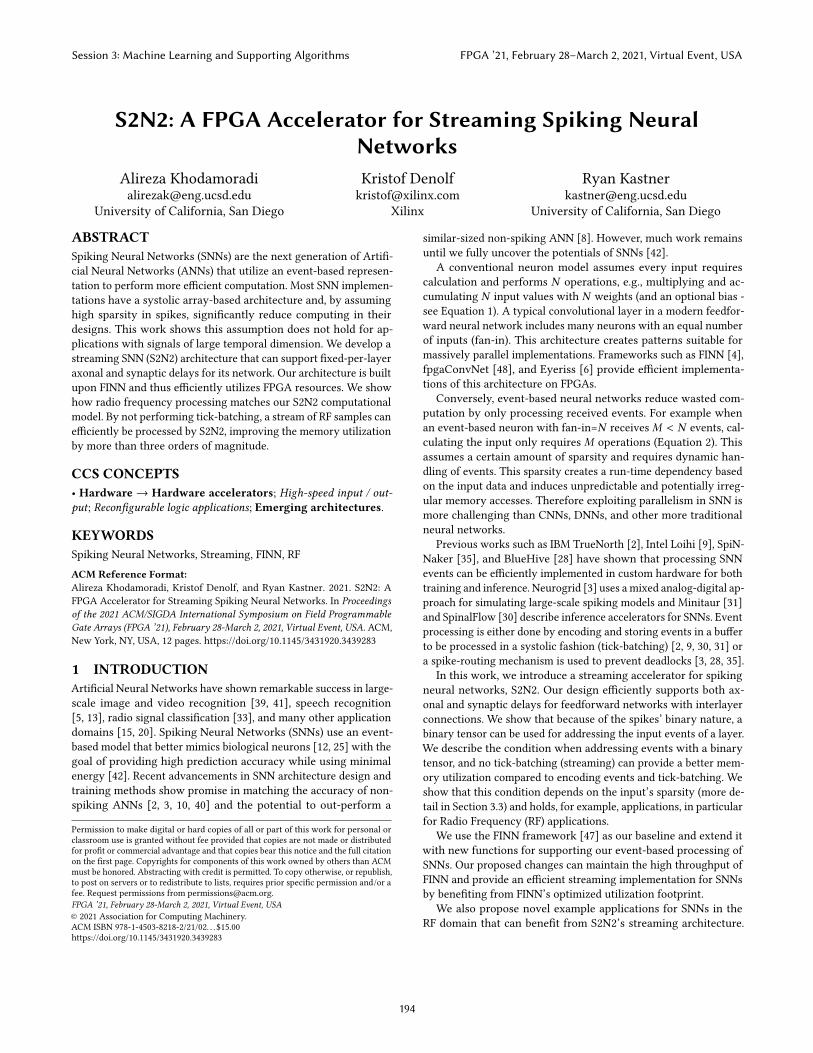
Figure 2: LIF neuron with two inputs. An incoming spike in-creases themembrane voltage by the weight associated withits connection. A decay parameter decreases the membranepotential, and if this voltage passes a threshold, it resets to apreset value, and the neuron generates a spike at its output.

𝑚𝑡 = (1 − out𝑡−1) ∗ 𝑑 ∗𝑚𝑡−1 + 𝐼𝑡 , 0 < 𝑑 < 1 (3)

out𝑡 =

{1, if 𝑚𝑡 > 𝑇

0, ow(4)

Here, 𝑑 ∈ (0, 1) is the decaying leak parameter, 𝑇 is the thresh-old,𝑚𝑡 is the membrane voltage at tick= 𝑡 , and 𝐼𝑡 is the input fromEquation 2. The term (1 − out𝑡−1) in Equation 3 is the reset mecha-nism that sets the membrane voltage to zero if neuron fires a spikein its output. This mechanism is illustrated in Figure 2.

Generally, training LIF neurons is done by treating the threshold(𝑇 ) and decay (𝑑) as non-trainable hyperparameters.

2.2 Propagation Delays in NeuronAs shown in Figure 3, a biological neuron has different components.Simply, nerve impulses are received by dendrites and processed bythe nucleus. Impulses generated by the neuron travel through theaxon and are distributed through synapses.

This process has two propagation delays: 1) Axonal delay thatis the time required for an action potential to travel from soma tosynapses through the axon. 2) Synaptic delay that is the time intervalrequired for a neurotransmitter to be released from a presynapticmembrane distribute across the synaptic cleft and received by thepost-synaptic membrane.

Supporting these propagation delays in implementation can in-crease the complexity of the design. Hence, only a few previousworks support these delays (more detail in the next section).

2.3 Custom SNN ImplementationsAnalog [22, 23, 44], digital [2, 7, 9, 28, 30, 31, 35, 45], and mixed-analog-digital [3, 29] accelerators for SNNs have been described inthe literature.

Analog realizations [22, 23, 44] are based on memristive tech-nology [43] and have to deal with latency, density, and variabilityissues related to this technology [1]. In an other work [29], in addi-tion to a memristive-based analog module, a digital module is usedto route events and update receptive neurons. Neurogrid [3] doesnot use memristive technology in its analog module and increases

Figure 3: Illustration of a biological neuron. Dendrites re-ceive inputs from presynaptic membranes to soma. The nu-cleus reacts to the received signals and may produce an ac-tion potential, which then has to go through the axon anddistribute to post-synaptic membranes through Synapses.

parallelism by using a digital router for its events. In this work, weintroduce a digital implementation for SNNs, and therefore we donot compare our work with analog realizations.

Large scale custom chip implementations such as Intel Loihi [9]with 4,096 on-chip cores and 1,024 neural units per core, SpiNNakersupercomputer [35] with 57,600 chips and 1,036,800 processors eachcapable of simulating 1,000 neurons, and IBM TrueNorth [2] with4,096 cores and supporting one million neurons are designed withsynaptic delay support. These implementations are designed to sup-port a mesh of neurons with no particular topology. This is done byusing advanced routers and schedulers. For example, Loihi uses sixbits for the synaptic delay and two independent physical routingnetworks for core-to-core multicast. And events in SpiNNaker arecoded to AER [26] packets (including timestamp, position, polarity,and debugging bits) and are source coded, meaning that the des-tination of each neuron has to be stored for routing the packets.TrueNorth has its own packet coding scheme, including the addressof the core, axon index, tick number, and debugging flags. It buffersthe events and uses a scheduler for processing events at specifiedticks for supporting the synaptic delay.

Previous FPGA implementations of SNNs took a similar ap-proach. BlueHive [28] is a 4-FPGA system and supports 64k Izhike-vich [16] neurons per FPGA. BlueHive uses a routing system forevents and 16 FIFOs for queuing events for 16 different synapticdelays with 1 millisecond granularity. Minitaur [31] encodes itsevents into five bytes, four bytes for timestamp and one byte forlayer index. It supports a fixed axonal delay by buffering its events.In some other implementations routing and queuing is done with-out supporting synaptic or axonal delays [7, 11, 30, 45]. Becauseof queuing, parallelism in these works is done when an event isprocessed. Each event has a number of destinations, and upon pro-cessing an event, all of its destinations (membrane potentials) areincremented by their associated weights in parallel. Routers andschedulers are used to prevent deadlocks and data hazards whileprocessing events from different queues with the same destinations.A comparison is provided at Table 1.

In the next section, we argue that by considering the networktopology, for a feedforward network with interlayer connections,fixed-per-layer axonal and synaptic delays can be supported with-out extra FIFOs, schedulers, and separate routing networks.

Session 3: Machine Learning and Supporting Algorithms FPGA ’21, February 28–March 2, 2021, Virtual Event, USA

196

Table 1: A comparison between S2N2 and previous works.

Architecture Technology Purpose Supported Topology Supported Propagation Delay Required Complexity for supporting delay

Loihi [9] custom chip training and simulation general mesh synaptic two separate physical routers

SpiNNaker [35] custom chip simulation general mesh synaptic AER packets+router

TrueNorth [2] custom chip simulation general mesh synaptic per-chip scheduler

BlueHive [28] FPGA simulation general mesh synaptic 16 FIFOs with 1ms granularity

Minitaur [31] FPGA accelerator general mesh fixed axonal tick-batching and sorting

SpinalFlow [30] FPGA accelerator feedforward none tick-batching (without supporting delays)

[45] FPGA accelerator small and dense none N/A

[7] FPGA accelerator feedforward none tick-batching (without supporting delays)

[11] FPGA accelerator feedforward none tick-batching (without supporting delays)

[17] FPGA accelerator feedforward none tick-batching (without supporting delays)

S2N2 FPGA accelerator feedforward synaptic+axonal streaming

3 STREAMING SPIKING NEURALNETWORKS (S2N2)

To explain the streaming architecture of S2N2, we first look into thecoding scheme used for storing events in input buffers. And explainthe condition when a binary tensor can utilize less memory. Wethen explain how feedforward SNNs with interlayer connectionscan support fixed-per-layer synaptic and axonal delays withoutrequiring schedulers and separate routing systems.

3.1 Input Buffer - Memory UtilizationAs shown in Figure 1, a spiking input has a temporal duration witha total number of ticks (time units). In tick-batching, all the eventsfor the entire duration of input are buffered and processed in asystolic implementation [30].

Let’s look at the input events in a layer of a feedforward network.Assuming 𝑆 being the total number of inputs to the layer, and𝑇 thetotal duration of the input, to encode events, we need log2 𝑆 bitsfor addressing the position and log2𝑇 bits for addressing the ticknumber of each event. Assuming sparsity in the incoming events,the layer can receive up to 𝑝 ∗𝑆𝑇 events when 𝑝 = 1−sparsity_ratioand 𝑝 ∈ (0, 1). Therefore we need a buffer of size:

buffer size in bits = 𝑝𝑆𝑇 log2 𝑆𝑇 (5)

On the other hand, we can use a binary tensor to address theinput events, ones for when there is an event, and zeros otherwise.In this case, we need 𝑆𝑇 -bits to store addresses in a binary tensor.Buffering encoded events requires less memory compared to abinary tensor if:

𝑝 log2 𝑆𝑇 < 1 (6)

This can be a tight condition on input’s sparsity. E.g., for a layerwith an input tensor of size 64 × 16 × 16 with a total duration of 16ticks, only for 𝑝 < 1

18 = 5.5% or 94.5% sparsity for input, bufferingencoded events uses less memory compared to a binary tensor ofsize 218 bits. In this example, as soon as the input’s sparsity dropsbelow 94.5%, Equation 6 is not satisfied, and the binary tensor

requires less memory. In Sections 4 and 5, we show that Equation 6can not be satisfied for our applications.

3.2 Fixed-Per-Layer Propagation Delays

Figure 4: Top: A simple 3-layer networkwith fixed-per-layeraxonal and synaptic delays. Inputs to each layer are binaryvectors, and "1"s are for spikes. Input to a neuron is thesum of all inputs, and all weights are equal to one. Bottom:the flow of the input through the network. E.g., network in-put at tick=1 (color-coded) is received by both neurons inthe first layer. With no axonal delay, they each produce onespike at their outputs at the same tick. The second layer re-ceives this input (same color code) with a synaptic delay (3ticks). At tick=4, both inputs to each neuron in the secondlayer have spikes. Hence their inputs are equal to 2.

As mentioned before, synaptic delays are realized in a limitednumber of previous work. Custom chips [2, 9, 35] queue their events

Session 3: Machine Learning and Supporting Algorithms FPGA ’21, February 28–March 2, 2021, Virtual Event, USA

197

and use complex routing and scheduling systems to process eventsat the correct tick with an appropriate delay. In FPGA implemen-tations, multiple FIFOs are used to support synaptic delays withlarge granularity (1 millisecond) [28]. These implementations sup-port different topologies of spiking networks. And [31] supportsfeedforward networks with fixed axonal delays by buffering andsorting its encoded events.

Feedforward SNNs with interlayer connections have a specifictopology that can be exploited for supporting fixed-per-layer synap-tic and axonal delays with a reduced implementation cost. As shownin [49], temporal coding is still possible with fixed propagation de-lays. Figure 4 shows a simple 3-layer network with fixed-per-layeraxonal and synaptic delays, meaning that all neurons in one layerhave the same axonal delay and the same synaptic delay. For thesake of simplicity, neurons in this network spike if they receive aninput larger than zero, and all weights are equal to one. Input toeach neuron is the sum of all inputs.

The bottom part of Figure 4 shows how spikes spread through thenetwork under axonal and synaptic delay conditions. Input to eachlayer is a binary vector, and spikes are represented by "1"s. Weightsare equal to one, and input to a neuron is the sum of weights forconnections with a spike. E.g. at tick=4, both inputs to neuron 10have spikes and in(10) = 2. Previous works with propagation delaysupport [2, 9, 28, 31, 35] support this with different complexities(see Table 1).

Figure 5: With fixed-per-layer propagation delays in the ex-ample network shown in Figure 4, we can process inputs andoutputs of all layers assuming no delay and push all the de-lays to the end. Then an accumulated delay (shown in purpleand blue) can be added to the network output.

However, because of the network topology, we can process allthe layers, assuming no propagation delay, and push all the delaysto the end. Then a total delay equal to all accumulated delays canbe applied to the network’s output as shown in Figure 5.

This practice can be applied to any structured feedforward net-work with only interlayer connections. In this case, we can supportboth synaptic and axonal delays without schedulers, extra FIFOs,and sorting mechanisms used in previous works.

3.3 ArchitectureThe streaming architecture of S2N2 is designed based on the FINNframework [47]. In the following, we first describe FINN’s approachto implementing non-spiking and conventional neural networks.We then describe our design to support the LIF model in FINN.

FINN framework: The original FINN paper [47] introduced aframework for building fast and flexible FPGA accelerators using a

flexible heterogeneous streaming architecture. Exploiting a set ofoptimizations, FINN enables efficient mapping of binarized neuralnetworks to hardware and supports fully connected, convolutional,and pooling layers. The second version of FINN described in [4],provides support for non-binary networks.

In the FINN architecture, a Sliding Window Unit (SWU) preparesthe input by applying interleaving and implementing the image-to-column (im2col) algorithm. The output stream of a SWU feedsa Matrix Vector Threshold Unit (MVTU), which is the computa-tional core for FINN’s accelerator designs. This core is used in theimplementations of both fully connected and convolution layers.

As shown in Figure 6, a MVTU has several Processing Elements(PE) that can generate output channels in parallel. Each PE has anumber of SIMD lanes. If 𝑃FINN be the number of PEs and 𝑆FINN bethe number of SIMD lanes, A 𝑃FINN-high, 𝑆FINN-wide tile matrixis processed at a time, inputs are mapped to different SIMD lanesand outputs are calculated in parallel by PEs. To accommodate thisprocess, weights are also loaded from memory in tiles, and each PEtakes a sub-tile of the weights to process its output.

All PE units have access to the input buffer inside the MVTU.The width of this buffer in bits is equal to the number of SIMD lanesmultiplied by the activation bit width. For simplicity, only one rowof this buffer is shown in Figure 6. The total number of rows in thisbuffer is equal to the ratio of (kernel width × kernel height × #inputchannels)/#SIMD lanes. Which makes the input buffer size equal to(kernel width × kernel height × #input channels) for 1-bit activation.

Figure 6: FINN [47] architecture. SWU interleaves the in-put by applying the image-to-column algorithm and feedsMVTU. Each PE inside MVTU processes one output channeland has a number of SIMD lanes that read from input chan-nels and multiply the input by kernel weights in parallel.

Session 3: Machine Learning and Supporting Algorithms FPGA ’21, February 28–March 2, 2021, Virtual Event, USA

198

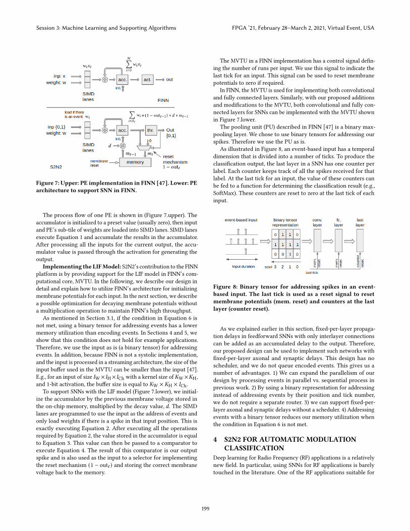
Figure 7: Upper: PE implementation in FINN [47]. Lower: PEarchitecture to support SNN in FINN.

The process flow of one PE is shown in (Figure 7.upper). Theaccumulator is initialized to a preset value (usually zero), then inputand PE’s sub-tile of weights are loaded into SIMD lanes. SIMD lanesexecute Equation 1 and accumulate the results in the accumulator.After processing all the inputs for the current output, the accu-mulator value is passed through the activation for generating theoutput.

Implementing the LIFModel: S2N2’s contribution to the FINNplatform is by providing support for the LIF model in FINN’s com-putational core, MVTU. In the following, we describe our design indetail and explain how to utilize FINN’s architecture for initializingmembrane potentials for each input. In the next section, we describea possible optimization for decaying membrane potentials withouta multiplication operation to maintain FINN’s high throughput.

As mentioned in Section 3.1, if the condition in Equation 6 isnot met, using a binary tensor for addressing events has a lowermemory utilization than encoding events. In Sections 4 and 5, weshow that this condition does not hold for example applications.Therefore, we use the input as is (a binary tensor) for addressingevents. In addition, because FINN is not a systolic implementation,and the input is processed in a streaming architecture, the size of theinput buffer used in the MVTU can be smaller than the input [47].E.g., for an input of size 𝐼W× 𝐼H× 𝐼Ch with a kernel size of 𝐾W×𝐾H,and 1-bit activation, the buffer size is equal to 𝐾W × 𝐾H × 𝐼Ch.

To support SNNs with the LIF model (Figure 7.lower), we initial-ize the accumulator by the previous membrane voltage stored inthe on-chip memory, multiplied by the decay value, 𝑑 . The SIMDlanes are programmed to use the input as the address of events andonly load weights if there is a spike in that input position. This isexactly executing Equation 2. After executing all the operationsrequired by Equation 2, the value stored in the accumulator is equalto Equation 3. This value can then be passed to a comparator toexecute Equation 4. The result of this comparator is our outputspike and is also used as the input to a selector for implementingthe reset mechanism (1 − out𝑡 ) and storing the correct membranevoltage back to the memory.

The MVTU in a FINN implementation has a control signal defin-ing the number of runs per input. We use this signal to indicate thelast tick for an input. This signal can be used to reset membranepotentials to zero if required.

In FINN, the MVTU is used for implementing both convolutionaland fully connected layers. Similarly, with our proposed additionsand modifications to the MVTU, both convolutional and fully con-nected layers for SNNs can be implemented with the MVTU shownin Figure 7.lower.

The pooling unit (PU) described in FINN [47] is a binary max-pooling layer. We chose to use binary tensors for addressing ourspikes. Therefore we use the PU as is.

As illustrated in Figure 8, an event-based input has a temporaldimension that is divided into a number of ticks. To produce theclassification output, the last layer in a SNN has one counter perlabel. Each counter keeps track of all the spikes received for thatlabel. At the last tick for an input, the value of these counters canbe fed to a function for determining the classification result (e.g.,SoftMax). These counters are reset to zero at the last tick of eachinput.

Figure 8: Binary tensor for addressing spikes in an event-based input. The last tick is used as a reset signal to resetmembrane potentials (mem. reset) and counters at the lastlayer (counter reset).

As we explained earlier in this section, fixed-per-layer propaga-tion delays in feedforward SNNs with only interlayer connectionscan be added as an accumulated delay to the output. Therefore,our proposed design can be used to implement such networks withfixed-per-layer axonal and synaptic delays. This design has noscheduler, and we do not queue encoded events. This gives us anumber of advantages. 1) We can expand the parallelism of ourdesign by processing events in parallel vs. sequential process inprevious work. 2) By using a binary representation for addressinginstead of addressing events by their position and tick number,we do not require a separate router. 3) we can support fixed-per-layer axonal and synaptic delays without a scheduler. 4) Addressingevents with a binary tensor reduces our memory utilization whenthe condition in Equation 6 is not met.

4 S2N2 FOR AUTOMATIC MODULATIONCLASSIFICATION

Deep learning for Radio Frequency (RF) applications is a relativelynew field. In particular, using SNNs for RF applications is barelytouched in the literature. One of the RF applications suitable for

Session 3: Machine Learning and Supporting Algorithms FPGA ’21, February 28–March 2, 2021, Virtual Event, USA

199

ANNs is Automatic Modulation Classification (AMC). This impor-tant method can be used in radio fault detection, opportunisticmesh networking, dynamic spectrum access, and numerous regu-latory and defense applications. Previous works have shown thatANNs can effectively perform modulation classification with highaccuracy [24, 27, 32, 34].

This section introduces two new network architectures for AMCthat are based on S2N2. The novelty of these architectures is thatthe input is fed to the network as a stream of events in the In-phase/Quadrature (I/Q) plane. To our knowledge, these are the onlyneural networks that consume a stream of RF samples as an event-based input. In the following, we describe the datasets used fortraining and explain our networks’ architecture.

Datasets: We use two RF datasets to train our networks. Ra-dioML.2016 [32] is a collection of 11 different modulations (8PSK,AM-DSB, AM-SSB, BPSK, CPFSK, GFSK, PAM4, QAM16, QAM64,QPSK, and WBFM). Each class has samples recorded at 20 differentSignal to Noise Ratio (SNR) levels (from -20dB to 18dB in incrementsof 2dB). Each pair {modulation, SNR} has 728 training examples, andEach training example is a time-series of 128 In-phase Quadrature(I/Q) sample pairs.

RadioML.2018 [34] is a collection of 24 different modulations(OOK, 4ASK, 8ASK, BPSK, QPSK, 8PSK, 16PSK, 32PSK, 16APSK,32APSK, 64APSK, 128APSK, 16QAM, 32QAM, 64QAM, 128QAM,256QAM, AM-SSBWC, AM-SSB-SC, AM-DSB-WC, AM-DSB-SC,FM, GMSK, andOQPSK). Eachmodulation class has samples recordedat 26 different SNR levels (from -20dB to 30dB in increments of 2dB).Each pair {modulation, SNR} has 4096 training examples and Eachtraining example is a time-series of 1024 I/Q sample pairs. Bothdatasets are publicly available 2.

Two time-series examples from RadioML.2018 are shown in Fig-ure 9.left. These examples are 1024 I/Q sample pairs. In all of theprevious work, inputs are tensors with same shape as these exam-ples. E.g., for RadioML.2016, inputs are 2 × 128 float tensors, and inRadioML.2018, inputs are 2 × 1024 float tensors.

S2N2 is not a systolic implementation. Meaning, we can feed thenetwork with a stream of events. Therefore, in our networks, weuse the constellation of signals (shown in Figure 9.middle), and ateach tick, we feed the network with one sample (Figure 9.right).Therefore our input is a stream of binary tensors.

To our knowledge feeding RF samples as events to a neuralnetwork has never been done before. The only work on using SNNsfor AMC is a preliminary investigation done by NASA [19] thatimplements a two-layer SNN in MATLAB for classifying threenoise-free modulations (BPSK, QPSK, and 8PSK). In NASA’s work,inputs are 8-bit images of constellations.

Feeding a neural network with RF samples as events come withtwo benefits. 1) Althoughwe and all the previousworks use recordeddata, in a real-world setup, our network can consume RF samplesone-by-one in a stream. Other works have to buffer samples (e.g.,128 or 1024 samples) before taking them as input. 2) We can aggres-sively quantize the I/Q plane; therefore the input size (in bits) canget smaller. The following explains the I/Q plane quantization.

Examples in RadioML.2016 and RadioML.2018 are 128 and 1024pairs of float numbers, respectively. We construct the I/Q plane by

2https://www.deepsig.ai/datasets

Figure 9: Examples of AM-DSB class from RadioML dataset[34]. On the left, two examples of AM-DSB I/Q samples areshown at 30dB and 2dB SNR at top and bottom, respectively.The middle illustrates the constellations of the same exam-ples. On the right, input to the network at time (tick)=𝑡 isshown. Input to our networks are samples as events in I/Qplane.

Figure 10: Applying quantization to the I/Q plane. Originalexamples from RadioML.2018 [34] dataset are 1024 pairs offloat numbers (left). In-phase and Quadrature values can bequantized for a smaller input tensor (first three columnsfrom the right). At each tick, we feed one slice of the quan-tized constellation tensor to the network. The figure showsthat the constellation shape is recognizable while I/Q planeis aggressively quantized.

quantizing the pair using a uniform quantizer. This will reduce ourinput size. Figure 10 illustrates three examples from RadioML.2018:OOK, 64QAM, and 32PSK classes at 30db, 16dB, and 2dB SNR, re-spectively. To the right of these examples, their constellations withquantized in-phase and quadrature values are shown. As it is shown,the shapes of the constellations are recognizable even at the lowestbit resolution. We used the 4-bit quantized constellations to trainour networks.

Session 3: Machine Learning and Supporting Algorithms FPGA ’21, February 28–March 2, 2021, Virtual Event, USA

200

Network Architecture for RadioML.2016This network is a four layer architecture similar to the networkdescribed in [32] with different number of kernels and LIF modelfor activation (Figure 11).

Figure 11: S2N2_rf1 architecture.

Inputs to each layer are binary tensors. We used 90% of thedataset for training and 10% for validation. For training, we used themethod described in [37] as our baseline and changed the loss func-tion to smooth L1 loss, and adjusted the hyperparameters. Through-out this paper, we refer to this network as S2N2_rf1.

Table 2: Comparing validation accuracy andnetwork size forS2N2_rf1.

Network Input Conv.1 Conv.2 Dense 1 Dense 2 Accuracy

[32] 128x2 64x1x3 16x2x3 128 11 87.4%32-bit

S2N2_rf1 16x16 16x5x5 8x5x5 128 11 91.7%binary

We achieved 91.7% Top-1 and 100% Top-5 validation accuracy us-ing all SNR levels in our training. A comparison between S2N2_rf1’ssize and accuracy with the previous work on RadioML.2016 is pro-vided in Table 2.

Figure 12 illustrates the spike ratio in the input of each layer forS2N2_rf1. The first convolution layer (Conv.1) receives one eventat each tick; this means that the spike ratio for this layer with aninput of size 16 × 16 is 1

16×16 = 0.0039.

Table 3: Required memory for buffering input at each layerof S2N2_rf1 is compared with tick-batching (Equation 5).

Layer #Ticks Input Size Maximum Buffer Size Buffer Size ImprovementSpike Ratio Tick-Batching S2N2_rf1

Conv.1 128 16×16 0.39% 1,917 bits 25 bits ×77Conv.2 128 16×16×16 7% 697,304 bits 400 bits ×1,744Dense 1 128 8×12×12 8% 212,337 bits 128 bits ×1,658Dense 2 128 128 12% 27,526 bits 11 bits ×2,502

As mentioned in Sections 2.3 and 3.1, previous works have usedtick-batching and buffered encoded events. This means that for atotal number of ticks=128, and input size of 16 × 16 at spike rationof 0.39%, according to Equation 5, tick-batching requires 1,917 bitsto queue the input events. Because S2N2 is based on the streaming

Figure 12: The ratio of spiking neurons in input to each layerof S2N2_rf1. Ratios are collected during classifying one in-put (128 ticks) with trained weights.

architecture of FINN [47], and only a portion of the input is bufferedfor processing. The size of this buffer used in MVTU is equal tokernel size × #input channels=25 bits for Conv.1 layer. In Table 3,we provide the same comparison for all the layers of this network.These results show that, on average, memory utilization for inputbuffers in S2N2_rf1 is improved by over three orders of magnitude.

Network Architecture for RadioML.2018As mentioned in our introduction, training methods for spikingneural networks are not as mature as other ANNs. In particular,current training methods are evaluated on smaller networks, andsimple datasets [11] and perform poorly when used for trainingvery deep architectures [18, 40] and evaluated on more complexdatasets [38]. Therefore we could not train a deep spiking networksimilar to the non-spiking networks used in previous works (VGG10and Resnet33) [34, 46]. Instead, we chose a smaller network withonly eight layers. We refer to this network as S2N2_rf2.

Figure 13: S2N2_rf2 architecture.

S2N2_rf2 architecture is shown in Figure 13. We used the sametraining script like the one we used for training S2N2_rf1 as thebaseline.We then adjusted the script for the dataset and its increasednumber of labels.

This network can achieve 68.5% Top-1 and 95% Top-5 validationaccuracy on 24 classes in RadioML.2018 dataset. Table 4 comparesour accuracy with two related non-spiking networks.

Although that S2N2_rf2 does not have a high accuracy comparedto deeper and non-spiking networks, it is included in this work toprovide a comparison between S2N2 architecture and tick-batching

Session 3: Machine Learning and Supporting Algorithms FPGA ’21, February 28–March 2, 2021, Virtual Event, USA

201

with regards to memory utilization. In particular, when larger RFinputs are used.

Table 4: Comparing validation accuracy andnetwork size forS2N2_rf2.

Network Input #Layers Accuracy

ResNet [34] 1024x2 (32-bit) 33 95.5%

VGG [34] 1024x2 (32-bit) 10 88.0%

S2N2_rf2 16x16 (binary) 6 68.5%

Figure 14 shows spike rations at the input of each layer ofS2N2_rf2. These ratios are similar to the ratios in S2N2_rf1 (Figure12). We expect that with future improvements in training methodsfor deeper SNNs, similar spike ratios with no significant reductionswill hold for a spiking network with a higher accuracy.

We use these ratios to show the efficiency of S2N2 for reducingthe input buffer size at each layer. Even if our assumption does nothold, and in the future networks with lower spike ratios provide ahigher accuracy, S2N2 is still more efficient at the minimum possiblespike ratio; only one spike at layer’s input (first row in Tables 3 and5).

Figure 14: The ratio of spiking neurons in input to each layerof S2N2_rf2. Ratios are collected during classifying one in-put (1024 ticks) with trained weights.

Table 5 illustrates a comparison between input buffer sizes re-quired for S2N2 and tick-batching. Equation 5 is used to calculatethe buffer size for tick-batching. It is clear that for inputs with largetemporal dimension, using a streaming architecture significantlyreduces the memory utilization.

Synthesis ResultsWe used Vivado-HLS™tool for evaluating S2N2_rf1 and S2N2_rf2network architectures. To increase the throughput and reduce ourDSP utilization, we used fixed-points for our parameters and trainedboth networks with a decay factor equal to 0.875 (𝑑 in Equation 3).This way, 𝑑 ×𝑚𝑡−1 in Figure 7 can be replaced by (𝑚𝑡−1 −𝑚𝑡−1 >>

3).

Table 5: Required memory for buffering input at each layerof S2N2_rf2 is compared with tick-batching (Equation 5).

Layer #Ticks Input Size Maximum Buffer Size Buffer Size ImprovementSpike Ratio Tick-Batching S2N2_rf2

Conv.1 1024 16×16 0.39% 18,403 bits 25 bits ×737Conv.2 1024 16×16×64 0.5% 2,013,266 bits 1,600 bits ×1,258Conv.3 1024 12×12×64 6% 13,589,545 bits 576 bits ×23,592Conv.4 1024 10×10×128 12% 37,748,736 bits 1,152 bits ×32,768Dense 1 1024 10×10×128 14% 44,040,192 bits 1,024 bits ×43,008Dense 2 1024 1024 5% 1,048,576 bits 24 bits ×43,690

We could fit S2N2_rf1 (smaller network) on a ZYNQ chip similarto the one used in the PYNQ development board. Because of thelarge size of S2N2_rf2, we selected the ZCU111 development boardin our synthesis. This board is also used for implementing a non-spiking network for the same dataset [46].

Table 6: Synthesis results for S2N2_rf1 and S2N2_rf2 net-work architectures.

Network Board BRAM_18K DSP48E FF LUT Tick Resolution

S2N2_rf1 PYNQ 29% 5% 11% 52% 45 ns

S2N2_rf2 ZCU111 98% <1% 4% 24% 30 ns

Our results are shown in Table 6. The high BRAM utilization isdue to the required memory for storing membrane potentials. Tickresolution indicates how fast RF samples can be consumed by thenetwork. E.g., at each second, S2N2_rf1 can classify 173.6k examplesfrom the RadioML.2016 dataset (each example requires 128 ticks).And S2N2_rf2 can process 32.5k examples from the RadioML.2018dataset (each example requires 1024 ticks).

5 IMAGE CLASSIFICATION ON S2N2In this section, we provide an example network for image clas-sification on MNIST dataset 3. We used the method provided byDECOLLE [18] to convert MNIST dataset to trains of spikes 4. Weused a four-layer convolutional network similar to the one describedin DECOLLE as our baseline.

Figure 15.left shows the network structure we used for imageclassification. We refer to this network as S2N2_cv. We appliedtwo modifications to the original structure. First, as shown in thefigure, in the original network, convolutional filters are appliedto the membrane voltage. This means MAC operations similarto Equation 1. We modified the layer, and instead, we apply theconvolutional filters on the input to have the sparse accumulationssimilar to Equation 2. Second, the neuron model used in the originalwork is a LIF model with two internal variables. We changed themodel to the one variable LIF model described in Section 2.1.

S2N2_cv is trained with the original training script 4, and ad-justed hyperparameters. It can achieve competitive results com-pared to other works (see Table 7).

3http://yann.lecun.com/exdb/mnist/4https://github.com/nmi-lab/dcll

Session 3: Machine Learning and Supporting Algorithms FPGA ’21, February 28–March 2, 2021, Virtual Event, USA

202

Figure 15: S2N2_cv structure. On the left, four-layer struc-ture of the network. Orange box, original organization ofone convolutional layer. Green box, convolutional layermodified for S2N2.

Table 7: Accuracy result of S2N2_cv on MNIST compared tosimilar SNNs.

Network Architecture Validation Accuracy

S2N2_cv 28x28-16c7-24c7-32c7-10 98.5%

[18] 28x28-16c7-24c7-32c7-10 98.0%

[40] 28x28-12c5-2a-64c5-2a-10c 99.3%

Figure 16: The ratio of spiking neurons in input to each layerof S2N2_cv. Ratios are collected during classifying one input(500 ticks) with trained weights.

Figure 16 shows the spike ratios at the input of each layer inS2N2_cv. The method for converting MNIST data to trains of spikesused in [18] converts each image to a 28 × 28 × 500 binary tensorof spikes. Unlike RF samples, input to the first layer can have morethan one spike at each tick; therefore, for vision applications, theinput is less sparse. Consequently, the ratio of spikes at each layeris higher than the layers in S2N2_rf1 and S2N2_rf2.

With higher spike ratios, the buffer size for storing encodedevents in tick-batching rapidly grows. While the buffer size used

in S2N2 is independent of the input’s spike ratio. Table 8 shows acomparison between these two buffer sizes for S2N2_cv network.

Table 8: Required memory for buffering input at each layerof S2N2_cv is compared with tick-batching (Equation 5).

Layer #Ticks Input Size Maximum Buffer Size Buffer Size ImprovementSpike Ratio Tick-Batching S2N2_cv1

Conv.1 500 28×28 0.7% 5,2136 bits 49 bits ×1,064Conv.2 500 16×13×13 16% 4,542,720 bits 784 bits ×5,794Conv.2 500 24× 11 ×11 33% 10,062,360 bits 1,176 bits ×8,556Dense 500 32×4×4 41% 1,889,280 bits 10 bits ×188,928

Synthesis ResultsS2N2_cv is evaluated with Vivado-HLS™tool. This network is rel-atively small, and we can fit it on the PYNQ development board.Our results are shown in Table 9.

To reduce our DSP utilization, we took a similar approach aswhatwe did for training our two other networks and trained S2N2_cvwith a decay factor equal to 0.875 (𝑑 in Equation 3). This way,𝑑 ×𝑚𝑡−1 in Figure 7 is replaced with a shift and one subtractions(𝑚𝑡−1 −𝑚𝑡−1 >> 3).

Table 9: Synthesis results for S2N2_cv network architecture.

Network Board BRAM_18K DSP48E FF LUT Tick Resolution

S2N2_cv PYNQ 35% <1% 2% 6% 30 ns

The high BRAM utilization in Table 9 is because of the memoryrequired to store membrane potentials for the LIF model (Figure 7).

6 CONCLUSIONIn this work, we introduced a streaming accelerator for spikingneural networks, namely S2N2. We showed that in batch-ticking,the buffer size used for storing encoded events depends on theinput’s spike ratios. This method is used in previous work, assuminga low spike ratio in the input.We showed that this assumption couldbe a tight condition on input’s spike ratio. We then described howa binary tensor could address events and confirmed that a binarytensor with our streaming architecture requires less memory in ourexample applications.

We also described how to efficiently support axonal and synapticdelays in a feedforward SNN with only interlayer connections.By using binary tensors as inputs, we built our architecture uponFINN platform. We provided support for the LIF model in FINNand optional initialization of membrane potentials for each inputto support SNNs in FINN.

Our streaming SNN architecture is suitable for processing sig-nals of large temporal dimension. Two novel SNN architectures forAMC are introduced in this work. In addition, an example of imageclassification on a SNN is described. All example applications areevaluated with the Vivado-HLS™tool. Our results achieve a mini-mum tick-resolution of 30 ns. S2N2 reduces input buffers’ memoryutilization by more than three orders of magnitude.

Session 3: Machine Learning and Supporting Algorithms FPGA ’21, February 28–March 2, 2021, Virtual Event, USA

203

REFERENCES[1] Gina Adam, Ali Khiat, and Themis Prodromakis. 2018. Challenges hindering

memristive neuromorphic hardware from going mainstream. In Nature Commu-nications, Vol. 9. https://doi.org/10.1038/s41467-018-07565-4

[2] F. Akopyan, J. Sawada, A. Cassidy, R. Alvarez-Icaza, J. Arthur, P. Merolla, N.Imam, Y. Nakamura, P. Datta, G. Nam, B. Taba, M. Beakes, B. Brezzo, J. B. Kuang,R. Manohar, W. P. Risk, B. Jackson, and D. S. Modha. 2015. TrueNorth: Designand Tool Flow of a 65 mW 1 Million Neuron Programmable Neurosynaptic Chip.IEEE Transactions on Computer-Aided Design of Integrated Circuits and Systems34, 10 (2015), 1537–1557.

[3] B. V. Benjamin, P. Gao, E.McQuinn, S. Choudhary, A. R. Chandrasekaran, J. Bussat,R. Alvarez-Icaza, J. V. Arthur, P. A. Merolla, and K. Boahen. 2014. Neurogrid:A Mixed-Analog-Digital Multichip System for Large-Scale Neural Simulations.Proc. IEEE 102, 5 (2014), 699–716.

[4] Michaela Blott, Thomas B. Preußer, Nicholas J. Fraser, Giulio Gambardella, Ken-neth O’brien, Yaman Umuroglu, Miriam Leeser, and Kees Vissers. 2018. FINN-R:An End-to-End Deep-Learning Framework for Fast Exploration of QuantizedNeural Networks. ACM Trans. Reconfigurable Technol. Syst. 11, 3, Article 16 (Dec.2018), 23 pages. https://doi.org/10.1145/3242897

[5] William Chan, Navdeep Jaitly, Quoc Le, and Oriol Vinyals. 2015. Listen, attend,and spell. IEEE International Conference on Acoustic, Speech, and Signal Processing(ICASSP) (2015).

[6] Y. Chen, T. Krishna, J. S. Emer, and V. Sze. 2017. Eyeriss: An Energy-EfficientReconfigurable Accelerator for Deep Convolutional Neural Networks. IEEEJournal of Solid-State Circuits 52, 1 (2017), 127–138.

[7] Kit Cheung, Simon R Schultz, and Wayne Luk. 2012. A large-scale spiking neuralnetwork accelerator for FPGA systems. In International Conference on ArtificialNeural Networks. Springer, 113–120.

[8] I. M. Comsa, K. Potempa, L. Versari, T. Fischbacher, A. Gesmundo, and J. Alakui-jala. 2020. Temporal Coding in Spiking Neural Networks with Alpha SynapticFunction. In ICASSP 2020 - 2020 IEEE International Conference on Acoustics, Speechand Signal Processing (ICASSP). 8529–8533.

[9] M. Davies, N. Srinivasa, T. Lin, G. Chinya, Y. Cao, S. H. Choday, G. Dimou, P.Joshi, N. Imam, S. Jain, Y. Liao, C. Lin, A. Lines, R. Liu, D. Mathaikutty, S. McCoy,A. Paul, J. Tse, G. Venkataramanan, Y. Weng, A. Wild, Y. Yang, and H. Wang. 2018.Loihi: A Neuromorphic Manycore Processor with On-Chip Learning. IEEE Micro38, 1 (2018), 82–99.

[10] Steven K. Esser, Paul A. Merolla, John V. Arthur, Andrew S. Cassidy, Rathinaku-mar Appuswamy, Alexander Andreopoulos, David J. Berg, Jeffrey L. McKinstry,Timothy Melano, Davis R. Barch, Carmelo di Nolfo, Pallab Datta, Arnon Amir,Brian Taba, Myron D. Flickner, and Dharmendra S. Modha. 2016. Convolu-tional networks for fast, energy-efficient neuromorphic computing. Proceed-ings of the National Academy of Sciences 113, 41 (2016), 11441–11446. https://doi.org/10.1073/pnas.1604850113

[11] H. Fang, Z. Mei, A. Shrestha, Z. Zhao, Y. Li, and Q. Qiu. 2020. Encoding, Model,and Architecture: Systematic Optimization for Spiking Neural Network in FPGAs.In 2020 IEEE/ACM International Conference On Computer Aided Design (ICCAD).1–9.

[12] Samanwoy Ghosh-Dastidar and Hojjat Adeli. 2009. Third Generation NeuralNetworks: Spiking Neural Networks. In Advances in Computational Intelligence.Springer Berlin Heidelberg, Berlin, Heidelberg, 167–178.

[13] Alex Graves and Jaitly Navdeep. 2014. Towards end-to-end speech recognitionwith recurrent neural networks. In 2014 International Conference on MachineLearning (ICML), Vol. 14.

[14] Alan Hodgkin and AndrewHuxley. 1952. A quantitative description of membranecurrent and its application to conduction and excitation in nerve. In The Journal ofphysiology, Vol. 117. 500. Issue 4. https://doi.org/10.1113/jphysiol.1952.sp004764

[15] Zan Huang, Hsinchun Chen, Chia jung Hsu, Wun hwa Chen, and SoushanWu. 2004. Credit Rating Analysis With Support Vector Machines and NeuralNetworks: A Market Comparative Study.

[16] Eugene. Izhikevich. 2003. Simple model of spiking neurons. In Transactions onNeural Networks, IEEE, Vol. 14. 1569 – 1572.

[17] X. Ju, B. Fang, R. Yan, X. Xu, and H. Tang. 2020. An FPGA Implementation ofDeep Spiking Neural Networks for Low-Power and Fast Classification. NeuralComputation 32, 1 (2020), 182–204. https://doi.org/10.1162/neco_a_01245

[18] Jacques Kaiser, Hesham Mostafa, and Emre Neftci. 2020. Synaptic Plasticity Dy-namics for Deep Continuous Local Learning (DECOLLE). Frontiers in Neuroscience14 (2020), 424. https://doi.org/10.3389/fnins.2020.00424

[19] E. J. Knoblock and H. R. Bahrami. 2019. Investigation of Spiking Neural Networksfor Modulation Recognition using Spike-Timing-Dependent Plasticity. In 2019IEEE Cognitive Communications for Aerospace Applications Workshop (CCAAW).1–5.

[20] Chang W. Lee and Jung-A Park. 2001. Assessment of HIV/AIDS-related healthperformance using an artificial neural network. Information & Management 38, 4(2001), 231 – 238. https://doi.org/10.1016/S0378-7206(00)00068-9

[21] Jun Haeng Lee, Tobi Delbruck, and Michael Pfeiffer. 2016. Training Deep SpikingNeural Networks Using Backpropagation. Frontiers in Neuroscience 10 (2016), 508.

https://doi.org/10.3389/fnins.2016.00508[22] Beiye Liu, Yiran Chen, Btyant Wysocki, and Tingwen Huang. 2015. Reconfig-

urable Neuromorphic Computing System with Memristor-Based Synapse Design.Neural Processing Letters 41 (2015), 159–167. https://doi.org/10.1007/s11063-013-9315-8

[23] C. Liu, B. Yan, C. Yang, L. Song, Z. Li, B. Liu, Y. Chen, H. Li, Qing Wu, and HaoJiang. 2015. A spiking neuromorphic design with resistive crossbar. In 2015 52ndACM/EDAC/IEEE Design Automation Conference (DAC). 1–6.

[24] X. Liu, D. Yang, and A. E. Gamal. 2017. Deep neural network architectures formodulation classification. In 2017 51st Asilomar Conference on Signals, Systems,and Computers. 915–919.

[25] Wolfgang Maass. 1997. Networks of spiking neurons: the third generation ofneural network models. In 1997 Neural Networks, Vol. 10. 1659–1671.

[26] Misha Mahowald. 1994. An analog VLSI system for sterescopic vision. Kluwer,Boston, MA.

[27] G. J. Mendis, J. Wei, and A. Madanayake. 2016. Deep learning-based automatedmodulation classification for cognitive radio. In 2016 IEEE International Conferenceon Communication Systems (ICCS). 1–6.

[28] Simon W Moore, Paul J Fox, Steven JT Marsh, A Theodore Markettos, and AlanMujumdar. 2012. Bluehive-a field-programable custom computing machine forextreme-scale real-time neural network simulation. In 2012 IEEE 20th InternationalSymposium on Field-Programmable Custom Computing Machines. IEEE, 133–140.

[29] Surya Narayanan, Ali Shafiee, and Rajeev Balasubramonian. 2017. INXS: Bridgingthe throughput and energy gap for spiking neural networks. In 2017 InternationalJoint Conference on Neural Networks, IJCNN 2017, Anchorage, AK, USA, May 14-19,2017. IEEE, 2451–2459. https://doi.org/10.1109/IJCNN.2017.7966154

[30] Surya Narayanan, Karl Taht, Rajeev Balasubramonian, Edouard Giacomin, andPierre-Emmanuel Gaillardon. 2020. SpinalFlow: An Architecture and DataflowTailored for Spiking Neural Networks. In 2020 47th International Symposium onComputer Architecture (ISCA-47).

[31] Daniel Neil and Shih-Chii Liu. 2014. Minitaur, an event-driven FPGA-basedspiking network accelerator. IEEE Transactions on Very Large Scale Integration(VLSI) Systems 22, 12 (2014), 2621–2628.

[32] Timothy J. O’Shea, Johnathan Corgan, and T. Charles Clancy. 2016. ConvolutionalRadio Modulation Recognition Networks. In Engineering Applications of NeuralNetworks. Springer International Publishing, Cham, 213–226.

[33] T. J. O’Shea, T. Roy, and T. C. Clancy. 2018. Over-the-Air Deep Learning BasedRadio Signal Classification. IEEE Journal of Selected Topics in Signal Processing12, 1 (2018), 168–179.

[34] T. J. O’Shea, T. Roy, and T. C. Clancy. 2018. Over-the-Air Deep Learning BasedRadio Signal Classification. IEEE Journal of Selected Topics in Signal Processing12, 1 (2018), 168–179.

[35] E. Painkras, L. A. Plana, J. Garside, S. Temple, F. Galluppi, C. Patterson, D. R.Lester, A. D. Brown, and S. B. Furber. 2013. SpiNNaker: A 1-W 18-Core System-on-Chip for Massively-Parallel Neural Network Simulation. IEEE Journal ofSolid-State Circuits 48, 8 (2013), 1943–1953.

[36] Priyadarshini Panda and Kaushik Roy. 2016. Unsupervised regenerative learn-ing of hierarchical features in spiking deep networks for object recognition. InInternational Joint Conference on Neural Networks (IJCNN). 299 – 306. https://doi.org/10.1109/IJCNN.2016.7727212

[37] Ali Samadzadeh, Fatemeh Sadat Tabatabaei Far, Ali Javadi, Ahmad Nickabadi,and Morteza Haghir Chehreghani. 2020. Convolutional Spiking Neural Networksfor Spatio-Temporal Feature Extraction. arXiv:2003.12346 [cs.CV]

[38] Abhronil Sengupta, Yuting Ye, Robert Wang, Chiao Liu, and Kaushik Roy. 2019.Going Deeper in Spiking Neural Networks: VGG and Residual Architectures.Frontiers in Neuroscience 13 (2019), 95. https://doi.org/10.3389/fnins.2019.00095

[39] Pierre Sermanet, David Eigen, Xiang Zhang, Michael Mathieu, Rob Fergus, andYann LeCun. 2014. OverFeat: Integrated Recognition, Localization and Detectionusing Convolutional Networks. In 2014 International Conference on LearningRepresentations (ICLR).

[40] Sumit Bam Shrestha and Garrick Orchard. 2018. SLAYER: Spike Layer ErrorReassignment in Time. In Advances in Neural Information Processing Systems 31,S. Bengio, H.Wallach, H. Larochelle, K. Grauman, N. Cesa-Bianchi, and R. Garnett(Eds.). Curran Associates, Inc., 1419–1428. http://papers.nips.cc/paper/7415-slayer-spike-layer-error-reassignment-in-time.pdf

[41] Karen Simonyan and Andrew Zisserman. 2014. Very Deep Convolutional Net-works for Large-Scale Image Recognition. arXiv:1409.1556 [cs.CV]

[42] James Smith. [n.d.]. A Roadmap for Reverse-Architecting the Brain’s Neocortex. Fed-erated Computing Research Conference (FCRC). https://iscaconf.org/isca2019/slides/JE_Smith_keynote.pdf

[43] Dmitri Strukov, Gregory Snider, Duncan Stewart, and Stanley Williams. 2008.The missing memristor found. In Nature, Vol. 453. 80–83. https://doi.org/10.1038/nature06932

[44] T. Tang, L. Xia, B. Li, R. Luo, Y. Chen, Y. Wang, and H. Yang. 2015. Spiking neuralnetwork with RRAM: Can we use it for real-world application?. In 2015 Design,Automation Test in Europe Conference Exhibition (DATE). 860–865.

[45] David Thomas and Wayne Luk. 2009. FPGA accelerated simulation of biologi-cally plausible spiking neural networks. In 2009 17th IEEE symposium on field

Session 3: Machine Learning and Supporting Algorithms FPGA ’21, February 28–March 2, 2021, Virtual Event, USA

204

programmable custom computing machines. IEEE, 45–52.[46] S. Tridgell, D. Boland, P. H.W. Leong, R. Kastner, A. Khodamoradi, and Siddhartha.

2020. Real-time Automatic Modulation Classification using RFSoC. In 2020 IEEEInternational Parallel and Distributed Processing Symposium Workshops (IPDPSW).82–89.

[47] Yaman Umuroglu, Nicholas J. Fraser, Giulio Gambardella, Michaela Blott, PhilipLeong, Magnus Jahre, and Kees Vissers. 2017. FINN: A Framework for Fast, Scal-able Binarized Neural Network Inference. In Proceedings of the 2017 ACM/SIGDAInternational Symposium on Field-Programmable Gate Arrays (Monterey, Cali-fornia, USA) (FPGA ’17). Association for Computing Machinery, New York, NY,USA, 65–74. https://doi.org/10.1145/3020078.3021744

[48] S. I. Venieris and C. Bouganis. 2016. fpgaConvNet: A Framework for MappingConvolutional Neural Networks on FPGAs. In 2016 IEEE 24th Annual InternationalSymposium on Field-Programmable Custom Computing Machines (FCCM). 40–47.

[49] Thomas Voegtlin. 2006. Temporal Coding Using the Response Properties ofSpiking Neurons. In Proceedings of the 19th International Conference on Neu-ral Information Processing Systems (NIPS’06). MIT Press, Cambridge, MA, USA,1457–1464.

[50] Friedemann Zenke and Surya Ganguli. 2018. SuperSpike: Supervised Learningin Multilayer Spiking Neural Networks. Neural Computation (2018), 1514–1541.https://doi.org/10.1162/neco_a_01086

Session 3: Machine Learning and Supporting Algorithms FPGA ’21, February 28–March 2, 2021, Virtual Event, USA

205