S TU V W X

Y Z [ \ ] ^ _ Z ` ^

a b c d e f e g c b h i j k l b m n e o p e q l o q g r l o e s g c b b o f j c d e g c r o e l c t l c d e a d e g t g u v t g g e s c q c t b l w p s e e i e l c xy r f n t z q c t b l v e n q j x q l o e s c t h t z q c t b l u v t g z n q t i e s | s q o r q c e ~ z d b b n b s i x c d t g c d e g t g u o t g g e s c q c t b lq o d e s e g c b c d e s b t g t b l g b h y r s o r e l t e s g t c j g y b n t z j b l l c e p s t c j t l e g e q s z d q l o c d e r g e b hz b j s t p d c e o i q c e s t q n

¡ ¢ £ ¤ ¥ ¦ ¡ § £ ¨ © ¤ ¥ § ª ¥ ¥ £ « ¬ ­ ® ¯ ° ® ° ® ± ² ® ® ²© ³ ´ µ ¶ · ¸ ¹ º ¹ » ¹ º ¼ ¹ ½ ¾ ¿¥ À · Á  À ¥ À

© ³ ´ µ ¶ · ¸ ¹ º© ³ ´ µ ¶ · ¸ ¹ º Ã Ä Å Æ Ç Å Ä Ã Æ È

CHARGE OPTIMIZATION OF LITHIUM-ION BATTERIES FOR

ELECTRIC-VEHICLE APPLICATION

A Thesis

Submitted to the Faculty

of

Purdue University

by

Sourav Pramanik

In Partial Fulfillment of the

Requirements for the Degree

of

Master of Science in Engineering

May 2015

Purdue University

Indianapolis, Indiana

ii

I would like to dedicate this work to my family and my wife Neha Ratnalikar.

iii

ACKNOWLEDGMENTS

I would like to express my deepest appreciation to my committee chair, Profes-

sor Sohel Anwar, who has always been instrumental and articulate in guiding me

throughout the course of this research. He has continuously and persuasively con-

veyed the spirit of adventure in regard to research, and an excitement in regard to

teaching. Without his supervision and constant help this thesis would not have been

possible.

I would like to thank my committee members, Professor Tamar Wasfy and Pro-

fessor Lingxi Li, whose work demonstrated to me that concern for global affairs sup-

ported by an engagement in comparative literature and modern technology, should

always transcend academia and provide a quest for our times.

I would like to thank my wife Neha Ratnalikar for her support and motivation

throughout the course of this work. I would also like to thank Ms. Valerie Lim Diemer,

Mr. Mark Senn and Ms. Sara Vitaniemi for their help and assistance throughout the

tenure of my masters program. Last but not the least, I would like to thank all my

co-workers and friends who have always been a source of knowledge and inspiration

to me.

iv

PREFACE

With the advent of time and recent achievements in technology, there is a need

for efficient source and use of energy. Apart from conventional and traditional forms

of energy sources, there is a tremendous need for mobile high density energy sources

to provide sustainable forms of energy. Lithium Ion is one such promising technol-

ogy which has vast potentials to suffice the need of ever increasing energy demands.

Lithium ion has certain added benefits over other energy sources which gives it a

higher edge over other sources.

Thus said, there is a urge to design better controls to charge and discharge the

energy cells. In this work the challenges and methods of charging a Lithium Ion cell

is studied and a better method is proposed to add some benefit to the process. The

work is done to achieve a better performance in whole, rather than achieving only a

specific goal. In this work a method to charge a Lithium Ion cell is described which is

designed to charge the battery in shortest time while maintaining the chemistry and

structure of the battery intact, so that the battery is not degraded beyond a specific

limit. This helps in achieving a balanced performance while delivering efficiency along

with longevity.

v

TABLE OF CONTENTS

Page

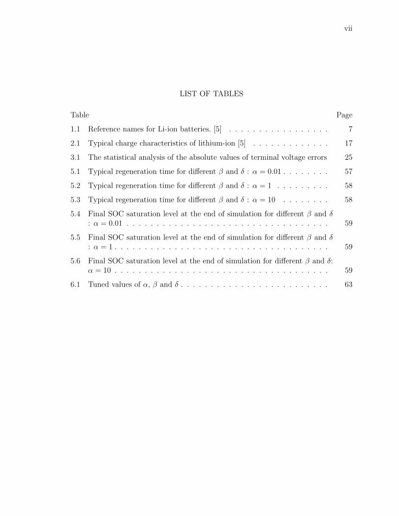
LIST OF TABLES . . . . . . . . . . . . . . . . . . . . . . . . . . . . . . . . vii

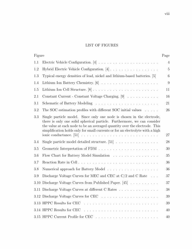
LIST OF FIGURES . . . . . . . . . . . . . . . . . . . . . . . . . . . . . . . viii

SYMBOLS . . . . . . . . . . . . . . . . . . . . . . . . . . . . . . . . . . . . x

ABBREVIATIONS . . . . . . . . . . . . . . . . . . . . . . . . . . . . . . . . xi

NOMENCLATURE . . . . . . . . . . . . . . . . . . . . . . . . . . . . . . . xiii

GLOSSARY . . . . . . . . . . . . . . . . . . . . . . . . . . . . . . . . . . . . xiv

ABSTRACT . . . . . . . . . . . . . . . . . . . . . . . . . . . . . . . . . . . xv

1 INTRODUCTION . . . . . . . . . . . . . . . . . . . . . . . . . . . . . . 1

1.1 Motivation and Major Contribution of this Thesis . . . . . . . . . . 1

1.2 Hybrid/Electric Vehicle Design . . . . . . . . . . . . . . . . . . . . 3

1.3 Lithium-Ion Cell structure . . . . . . . . . . . . . . . . . . . . . . . 5

1.3.1 Battery Chemistry . . . . . . . . . . . . . . . . . . . . . . . 6

1.3.2 Li Ion Battery Model . . . . . . . . . . . . . . . . . . . . . . 10

2 LITERATURE SURVEY . . . . . . . . . . . . . . . . . . . . . . . . . . . 15

2.1 Introduction . . . . . . . . . . . . . . . . . . . . . . . . . . . . . . . 15

2.2 Available Options . . . . . . . . . . . . . . . . . . . . . . . . . . . . 17

3 METHODOLOGY . . . . . . . . . . . . . . . . . . . . . . . . . . . . . . 19

3.1 Introduction . . . . . . . . . . . . . . . . . . . . . . . . . . . . . . . 19

3.2 Cell Model . . . . . . . . . . . . . . . . . . . . . . . . . . . . . . . . 19

3.2.1 Equivalent Circuit Model . . . . . . . . . . . . . . . . . . . . 24

3.2.2 Physics Based Cell Model . . . . . . . . . . . . . . . . . . . 24

3.2.3 Numerical Treatment of the Physics Based Cell Model . . . 27

4 OPTIMIZATION METHODS . . . . . . . . . . . . . . . . . . . . . . . . 43

4.1 Introduction . . . . . . . . . . . . . . . . . . . . . . . . . . . . . . . 43

vi

Page

4.2 Pontryagin’s Maximum/Minimum Principle . . . . . . . . . . . . . 43

5 PROBLEM FORMULATION AND SOLUTION TECHNIQUES . . . . . 47

5.1 Design Objectives . . . . . . . . . . . . . . . . . . . . . . . . . . . . 47

5.2 Problem Statement . . . . . . . . . . . . . . . . . . . . . . . . . . . 47

5.3 Performance Results . . . . . . . . . . . . . . . . . . . . . . . . . . 50

6 CONCLUSIONS AND RECOMMENDATIONS . . . . . . . . . . . . . . 62

6.1 Concluding Summary . . . . . . . . . . . . . . . . . . . . . . . . . . 62

6.2 Major contribution on the Thesis . . . . . . . . . . . . . . . . . . . 64

6.3 Recommendations for Future Work . . . . . . . . . . . . . . . . . . 65

LIST OF REFERENCES . . . . . . . . . . . . . . . . . . . . . . . . . . . . 66

APPENDICES

A REFERENCE FIGURES . . . . . . . . . . . . . . . . . . . . . . . . . . . 70

A.1 1-D Battery Model Numerical Solution Results . . . . . . . . . . . . 70

A.2 Tuning Results - Different α, β and δ Settings . . . . . . . . . . . . 77

B 1-D LITHIUM-ION BATTERY MODEL CODE . . . . . . . . . . . . . . 81

vii

LIST OF TABLES

Table Page

1.1 Reference names for Li-ion batteries. [5] . . . . . . . . . . . . . . . . . 7

2.1 Typical charge characteristics of lithium-ion [5] . . . . . . . . . . . . . 17

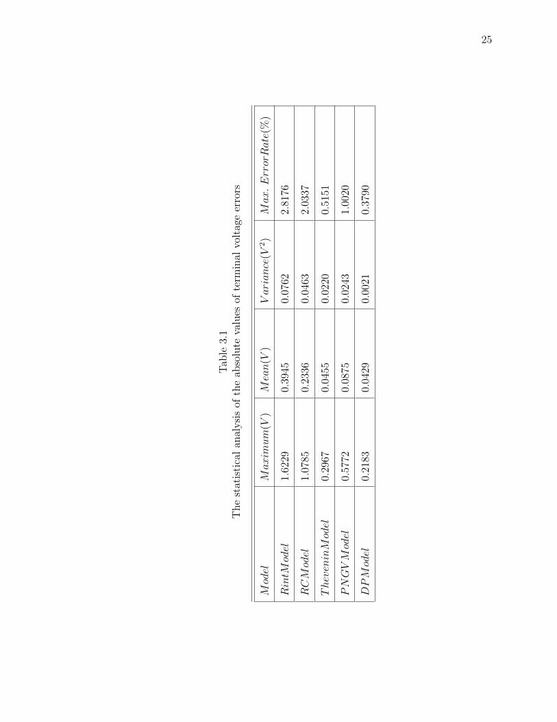
3.1 The statistical analysis of the absolute values of terminal voltage errors 25

5.1 Typical regeneration time for different β and δ : α = 0.01 . . . . . . . . 57

5.2 Typical regeneration time for different β and δ : α = 1 . . . . . . . . . 58

5.3 Typical regeneration time for different β and δ : α = 10 . . . . . . . . 58

5.4 Final SOC saturation level at the end of simulation for different β and δ: α = 0.01 . . . . . . . . . . . . . . . . . . . . . . . . . . . . . . . . . . 59

5.5 Final SOC saturation level at the end of simulation for different β and δ: α = 1 . . . . . . . . . . . . . . . . . . . . . . . . . . . . . . . . . . . . 59

5.6 Final SOC saturation level at the end of simulation for different β and δ:α = 10 . . . . . . . . . . . . . . . . . . . . . . . . . . . . . . . . . . . . 59

6.1 Tuned values of α, β and δ . . . . . . . . . . . . . . . . . . . . . . . . . 63

viii

LIST OF FIGURES

Figure Page

1.1 Electric Vehicle Configuration. [4] . . . . . . . . . . . . . . . . . . . . . 4

1.2 Hybrid Electric Vehicle Configuration. [4] . . . . . . . . . . . . . . . . . 5

1.3 Typical energy densities of lead, nickel and lithium-based batteries. [5] 6

1.4 Lithium Ion Battery Chemistry. [6] . . . . . . . . . . . . . . . . . . . . 9

1.5 Lithium Ion Cell Structure. [8] . . . . . . . . . . . . . . . . . . . . . . . 11

2.1 Constant Current - Constant Voltage Charging. [9] . . . . . . . . . . . 16

3.1 Schematic of Battery Modeling . . . . . . . . . . . . . . . . . . . . . . 21

3.2 The SOC estimation profiles with different SOC initial values . . . . . 26

3.3 Single particle model. Since only one node is chosen in the electrode,there is only one solid spherical particle. Furthermore, we can considerthe value at each node to be an averaged quantity over the electrode. Thissimplification holds only for small currents or for an electrolyte with a highionic conductance. [51] . . . . . . . . . . . . . . . . . . . . . . . . . . . 27

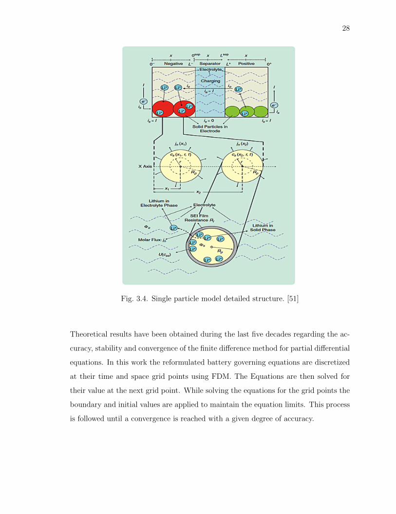
3.4 Single particle model detailed structure. [51] . . . . . . . . . . . . . . . 28

3.5 Geometric Interpretation of FDM . . . . . . . . . . . . . . . . . . . . . 30

3.6 Flow Chart for Battery Model Simulation . . . . . . . . . . . . . . . . 35

3.7 Reaction Rate in Cell . . . . . . . . . . . . . . . . . . . . . . . . . . . . 36

3.8 Numerical approach for Battery Model . . . . . . . . . . . . . . . . . . 36

3.9 Discharge Voltage Curves for MEC and CEC at C/2 and C Rate . . . 37

3.10 Discharge Voltage Curves from Published Paper. [45] . . . . . . . . . . 37

3.11 Discharge Voltage Curves at different C Rates . . . . . . . . . . . . . . 38

3.12 Discharge Voltage Curves for CEC . . . . . . . . . . . . . . . . . . . . 39

3.13 HPPC Results for CEC . . . . . . . . . . . . . . . . . . . . . . . . . . 39

3.14 HPPC Results for CEC . . . . . . . . . . . . . . . . . . . . . . . . . . 40

3.15 HPPC Current Profile for CEC . . . . . . . . . . . . . . . . . . . . . . 40

ix

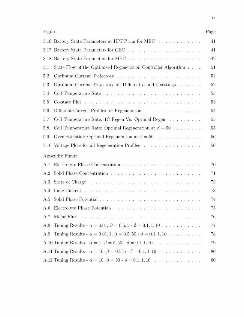
Figure Page

3.16 Battery State Parameters at HPPC run for MEC . . . . . . . . . . . . 41

3.17 Battery State Parameters for CEC . . . . . . . . . . . . . . . . . . . . 41

3.18 Battery State Parameters for MEC . . . . . . . . . . . . . . . . . . . . 42

5.1 State Flow of the Optimized Regeneration Controller Algorithm . . . . 51

5.2 Optimum Current Trajectory . . . . . . . . . . . . . . . . . . . . . . . 52

5.3 Optimum Current Trajectory for Different α and β settings . . . . . . 52

5.4 Cell Temperature Rate . . . . . . . . . . . . . . . . . . . . . . . . . . . 53

5.5 Co-state Plot . . . . . . . . . . . . . . . . . . . . . . . . . . . . . . . . 53

5.6 Different Current Profiles for Regeneration . . . . . . . . . . . . . . . . 54

5.7 Cell Temperature Rate: 1C Regen Vs. Optimal Regen . . . . . . . . . 55

5.8 Cell Temperature Rate: Optimal Regeneration at β = 50 . . . . . . . . 55

5.9 Over Potential: Optimal Regeneration at β = 50 . . . . . . . . . . . . . 56

5.10 Voltage Plots for all Regeneration Profiles . . . . . . . . . . . . . . . . 56

Appendix Figure

A.1 Electrolyte Phase Concentration . . . . . . . . . . . . . . . . . . . . . . 70

A.2 Solid Phase Concentration . . . . . . . . . . . . . . . . . . . . . . . . . 71

A.3 State of Charge . . . . . . . . . . . . . . . . . . . . . . . . . . . . . . . 72

A.4 Ionic Current . . . . . . . . . . . . . . . . . . . . . . . . . . . . . . . . 73

A.5 Solid Phase Potential . . . . . . . . . . . . . . . . . . . . . . . . . . . . 74

A.6 Electrolyte Phase Potentials . . . . . . . . . . . . . . . . . . . . . . . . 75

A.7 Molar Flux . . . . . . . . . . . . . . . . . . . . . . . . . . . . . . . . . 76

A.8 Tuning Results - α = 0.01, β = 0.5, 5 - δ = 0.1, 1, 10 . . . . . . . . . . . 77

A.9 Tuning Results - α = 0.01, 1, β = 0.5, 50 - δ = 0.1, 1, 10 . . . . . . . . . 78

A.10 Tuning Results - α = 1, β = 5, 50 - δ = 0.1, 1, 10 . . . . . . . . . . . . . 79

A.11 Tuning Results - α = 10, β = 0.5, 5 - δ = 0.1, 1, 10 . . . . . . . . . . . . 80

A.12 Tuning Results - α = 10, β = 50 - δ = 0.1, 1, 10 . . . . . . . . . . . . . 80

x

SYMBOLS

a inter-facial surface area

A cross-sectional area of an electrochemical cell

Ce,i concentration in electrolyte phase

Cs,i concentration in solid phase

De diffusion coefficient of electrolyte

Ds diffusion coefficient of solid

f+/− mean molar activity coefficient of electrolyte

F Faraday’s constant

in transfer current at the surface of active material

io exchange current density

Li thickness of electrode/separator

Q charge capacity

R universal gas constant

T temperature

αa, αc anodic and cathodic transfer coefficient

εi volume fraction

κi ionic conductivity in electrolyte

σi ionic conductivity in solid matrix

φs,i potential in solid matrix

φe,i potential in electrolyte

ρ material density

xi

ABBREVIATIONS

DOH degree of hybridization

EV electric vehicle

PHEV plug-in hybrid electric vehicle

GHG green house gases

ICE internal combustion engine

KKT Karush-Kuhn-Tucker

OCP open circuit potential

SEI solid electrolyte interface

SOC state of charge

DOD depth of discharge

SQP sequential quadratic programming

SNOPT Sparse Nonlinear OPTimizer

EUL End of Useful Life

PMP Pontryagin’s Minimum Principle

CEC Constant Electrolyte Concentration

MEC Modeled Electrolyte Concentration

PDAE Partial Differential Algebraic Equation

NMPC Non-Linear Model Predictive Control

EKF Extented Kalman Filter

ODE Ordinary Differential Equation

PDE Partial Differential Equation

SPM Single Particle Model

ROM Reduced Order Model

NOx Oxides of Nitrogen

xii

SOx Oxides of Sulphur

HC Hydrocarbons

BMS Battery management System

PWM Pulse Width Modulation

HJB Hamilton-Jacobi-Bellman

RC Resistance Capacitance

xiii

NOMENCLATURE

subscript i Refers to Positive/Negative Electrode

subscript n Refers to Negative Electrode

subscript p Refers to Positive Electrode

subscript s Refers to Separator Region

subscript e Refers to Electrolyte Phase

subscript s Refers to Solid Phase when not referring to separator

space node Refers to the iterative space steps

time node Refers to iterative time steps at which the numerical solution is

done

xiv

GLOSSARY

Cathode The Negative Terminal of the Battery. Electrons move

from this terminal to the Positive terminal during

regeneration process.

Anode The positive Terminal of the Battery. Lithium Ions

move from this terminal to the Negative Terminal

during regeneration of the battery.

Regeneration This is a term used to denote the state when energy is

supplied to the Battery. This is the state when the

battery is charged. It is called regeneration since the

cell is regenerated from a depleted state to a charged

state.

Regeneration Current This is the current which is applied to the cell during

a Battery Regeneration. This supplied current is

responsible to charge the battery.

Load Current This is the current which is drawn from the battery

during a discharge process. The battery can only

supply a rated load current for a rated time period

which is stated by the C Rate of the battery.

xv

ABSTRACT

Pramanik, Sourav. M.S.E., Purdue University, May 2015. Charge Optimization ofLithium-Ion Batteries for Electric-Vehicle Application. Major Professor: SohelAnwar.

In recent years Lithium-Ion battery as an alternate energy source has gathered lot

of importance in all forms of energy requiring applications. Due to its overwhelming

benefits over a few disadvantages Lithium Ion is more sought off than any other

Battery types. Any battery pack alone cannot perform or achieve its maximum

capacity unless there is some robust, efficient and advanced controls developed around

it. This control strategy is called Battery Management System or BMS. Most BMS

performs the following activity if not all - Battery Health Monitoring, Temperature

Monitoring, Regeneration Tactics, Discharge Profiles, History logging, etc. One of

the major key contributor in a better BMS design and subsequently maintaining a

better battery performance and EUL is Regeneration Tactics.

In this work, emphasis is laid on understanding the prevalent methods of regen-

eration and designing a new strategy that better suits the battery performance. A

performance index is chosen which aims at minimizing the effort of regeneration along

with a minimum deviation from the rated maximum thresholds for cell temperature

and regeneration current. Tuning capability is provided for both temperature devia-

tion and current deviation so that it can be tuned based on requirement and battery

chemistry and parameters. To solve the optimization problem, Pontryagin’s principle

is used which is very effective for constraint optimization with both state and input

constraints.

Simulation results with different sets of tuning shows that the proposed method

has a lot of potential and is capable of introducing a new dynamic regeneration tactic

xvi

for Lithium Ion cells. With the current optimistic results from this work, it is strongly

recommended to bring in more battery constraints into the optimization boundary to

better understand and incorporate battery chemistry into the regeneration process.

1

1. INTRODUCTION

1.1 Motivation and Major Contribution of this Thesis

In the last few centuries there has been a huge technological leap in all spheres of

human development. Transportation and automobile technologies have manifolded

along with this race for technological improvements. Due to modern high speed

transportation system, traveling across states and even overseas have become a piece

of cake. While these means of transportation allow us to reach all corners of the

world, they are energy intensive and depend primarily on fossil fuels. In the past half

century or so, our demand for fossil fuels has steadily climbed, as both the larger

population and their economic prosperity has increased [1].

These newer generation of automobiles consumes a large amount of fossil fuels and

along with increases the emission of green house gasses and other toxic life threatening

oxides (NOx, SOx, HCs, etc). GHG have been blamed as the main cause of anthro-

pogenic global warming. In 2011, transportation accounted for 28% of US primary

energy consumption, 93% of which came from petroleum [2]. This directly translates

to 28% of GHG emissions [3]. The ability to control the amount and the sources of

energy used for transportation can result in a significant reduction which accounted

for GHG release into the atmosphere as well.

The difficulties in controlling the GHG emissions and the over-dependence of fossil

fuels play major roles in shaping the future of transportation and pushed our limits to

venture out into other technological advancements to find alternative energy solutions.

The initiative to find alternative energy sources apart from conventional fossil fuels

for transport use, therefore, arises from the need to address the following concerns:

• Energy security: Reducing dependency on fossil fuels from foreign nations.

There is also the global risk of depleting the decreasing natural storage of fos-

2

sil fuels. There is a need to secure the future of fossil fuels and use it more

conservatively.

• Conservation: Sustain development without negatively impacting the envi-

ronment. Technological advancement and urbanization always push the natural

resources to limits. There has to be trade off between conserving the nature

and technological growth.

• Revenue protection: Maintain profitability and reduce the operating costs

by insulating against fluctuating fuel prices.

To address these issues, various green technologies, such as EVs and HEVs, advanced

battery technology, and alternative fuel systems, du fuel systems and even nuclear

technologies have gained prominence. The development has been most obvious in the

automotive industry, due to the need to improve vehicle fuel efficiency and to satisfy

increasingly stringent emission standards. Spurred by the feasibility of hydrogen fuel

cells and development of higher energy density batteries, EVs have been demonstrated

as possible successors of traditional vehicles operating with an internal combustion

engine (ICE). Various energy carriers are available to power EV of different archi-

tecture. Section 1.2 will explain various types of EVs and HEV’s, while Section 1.3,

talks more about Lithium Ion Cell Structure as an energy storage device. One of the

main advantages of electric-powered vehicles is the significantly lower operating costs

compared to ICE powered vehicles.

With this increasing trend towards utilizing more cleaner and alternate forms of

energy, Lithium Ion cells showcases a very high potential in the future years. Thus

there is a need to to develop a better controls around the usage and maintenance

of Lithium Ion battery management systems. This Thesis work is focused on un-

derstanding and studying Lithium Ion cell as an energy storage device, developing a

robust numerical framework to solve the reformulated 1-D model and verifying with

a published 1-D physics based cell model, and finally developing a robust charging

3

algorithm to charge the Lithium Ion cell in an efficient way. The major parts of the

Thesis are:

• Develop a robust 1-D Lithium Ion cell Model, which can replicate accurately

the battery reactions and phenomenon. The model is so chosen so that it is fast

enough in terms of computational speed along with maintaining the details of

chemistry so as not to lose any performance measures,

• Develop a robust algorithm to numerically solve the governing equations,

• Develop an efficient charging scheme which will not stress the battery beyond

its limits and will also charge it at a fast rate,

1.2 Hybrid/Electric Vehicle Design

Thus said, the need for alternate energy source to drive commercial vehicles is

widespread. There is a huge trend towards hybridization of automobile as well as off

road engines. Hybridization is also considered seriously these days for high volume

engines as well, along with light duty engines (passenger cars/ pickup vans). Hybrid

electric vehicles (HEVs) combine the benefits of gasoline engines and electric motors

and can be configured to meet different objectives such as improved fuel economy,

increased power, or additional auxiliary power for electronic devices and power tools.

HEVs run on fuel alone and do not plug in to an electrical outlet to recharge the

battery. The battery pack is charged utilizing engine power during regenerative brak-

ing. Though off course there are Plug-in HEV available which can be charged via, an

external charging outlet.

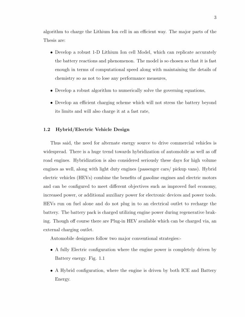
Automobile designers follow two major conventional strategies:-

• A fully Electric configuration where the engine power is completely driven by

Battery energy. Fig. 1.1

• A Hybrid configuration, where the engine is driven by both ICE and Battery

Energy.

4

Fig. 1.1. Electric Vehicle Configuration. [4]

Hybrid electric vehicles are powered by both internal combustion engine and elec-

tric motor independently or jointly, doubling the fuel efficiency compared with a

conventional vehicle. Hybrid passenger cars are achieving a substantial success in

sales in Japan and in the U.S. due to the features of high fuel efficiency, low emissions

and affordable price.

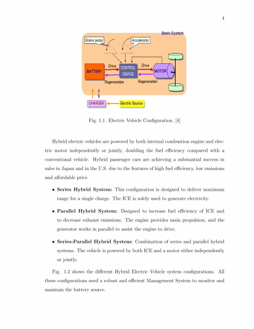
• Series Hybrid System: This configuration is designed to deliver maximum

range for a single charge. The ICE is solely used to generate electricity.

• Parallel Hybrid System: Designed to increase fuel efficiency of ICE and

to decrease exhaust emissions. The engine provides main propulsion, and the

generator works in parallel to assist the engine to drive.

• Series-Parallel Hybrid System: Combination of series and parallel hybrid

systems. The vehicle is powered by both ICE and a motor either independently

or jointly.

Fig. 1.2 shows the different Hybrid Electric Vehicle system configurations. All

these configurations need a robust and efficient Management System to monitor and

maintain the battery source.

5

Fig. 1.2. Hybrid Electric Vehicle Configuration. [4]

1.3 Lithium-Ion Cell structure

The focus of this thesis work is to develop a Lithium-Ion cell model and design

a robust charging scheme for the same. Before going into the details of charging

technique and algorithm ,a brief study of the Lithium-Ion cell is done in this section.

Lithium-ion has not yet reached its full maturity and the technology is continually

improving. The anode in today’s cell is made up of a graphite mixture and the

cathode is a combination of lithium and other choice of metals. All battery materials

has a theoretical energy density. With lithium-ion, the anode is well optimized and

little improvements can be gained in terms of design changes. The cathode, however,

shows promise for further enhancements. Battery research is therefore focusing on the

cathode material. Another scope of improvement in the battery cell is the electrolyte.

The electrolyte serves as a reaction medium between the anode and the cathode.

The battery industry is making incremental capacity gains of 8-10% per year.

This trend is expected to continue. This, however, is a far cry from Moore’s Law

that specifies a doubling of transistors on a chip every 18 to 24 months. Translating

this increase to a battery would mean a doubling of capacity every two years. In-

6

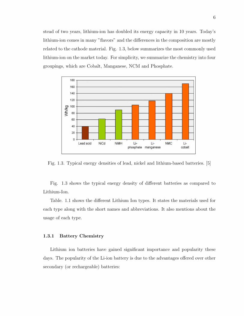
stead of two years, lithium-ion has doubled its energy capacity in 10 years. Today’s

lithium-ion comes in many ”flavors” and the differences in the composition are mostly

related to the cathode material. Fig. 1.3, below summarizes the most commonly used

lithium-ion on the market today. For simplicity, we summarize the chemistry into four

groupings, which are Cobalt, Manganese, NCM and Phosphate.

Fig. 1.3. Typical energy densities of lead, nickel and lithium-based batteries. [5]

Fig. 1.3 shows the typical energy density of different batteries as compared to

Lithium-Ion.

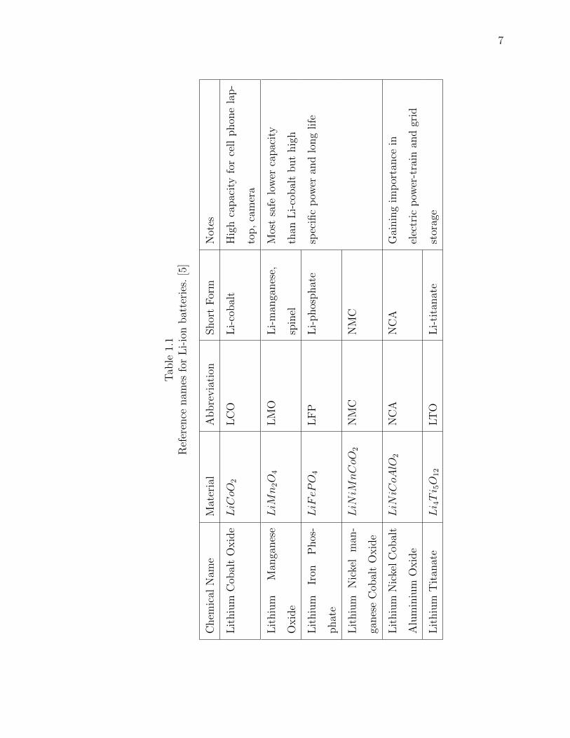
Table. 1.1 shows the different Lithium Ion types. It states the materials used for

each type along with the short names and abbreviations. It also mentions about the

usage of each type.

1.3.1 Battery Chemistry

Lithium ion batteries have gained significant importance and popularity these

days. The popularity of the Li-ion battery is due to the advantages offered over other

secondary (or rechargeable) batteries:

7

Tab

le1.

1R

efer

ence

nam

esfo

rL

i-io

nbat

teri

es.

[5]

Chem

ical

Nam

eM

ater

ial

Abbre

via

tion

Shor

tF

orm

Not

es

Lit

hiu

mC

obal

tO

xid

eLiCoO

2L

CO

Li-

cobal

tH

igh

capac

ity

for

cell

phon

ela

p-

top,

cam

era

Lit

hiu

mM

anga

nes

e

Oxid

e

LiM

n2O

4L

MO

Li-

man

ganes

e,

spin

el

Mos

tsa

felo

wer

capac

ity

than

Li-

cobal

tbut

hig

h

spec

ific

pow

eran

dlo

ng

life

Lit

hiu

mIr

onP

hos

-

phat

e

LiFePO

4L

FP

Li-

phos

phat

e

Lit

hiu

mN

icke

lm

an-

ganes

eC

obal

tO

xid

e

LiNiM

nCoO

2N

MC

NM

C

Lit

hiu

mN

icke

lC

obal

t

Alu

min

ium

Oxid

e

LiNiCoAlO

2N

CA

NC

A

Lit

hiu

mT

itan

ate

Li 4Ti 5O

12

LT

OL

i-ti

tanat

e

Gai

nin

gim

por

tance

in

elec

tric

pow

er-t

rain

and

grid

stor

age

8

• For the same given capacity Lithium Ion Batteries are much lighter than its

counterparts,

• Lithium ion chemistry delivers a high open-circuit voltage,

• Low self-discharge rate (about 1.5% per month),

• Do not suffer from battery memory effect,

• Environmental benefits: rechargeable and reduced toxic landfill.

Even though Lithium Ion Batteries have a lot of advantage over other rechargeable

batteries, they have certain disadvantages as well. Lithium Ion batteries have the

inherent issues such as:

• Poor cycle life, particularly in high current applications,

• Increase in internal resistance with cycling and aging,

• Safety concerns if overheated or overcharged,

• Applications which require a higher capacity are not designed to use Lithium

Ion Batteries,

• In Lithium Ion batteries, lithium ions move from the anode to cathode during

discharge, and from cathode to anode when charging. The materials used for the

anode and cathode can dramatically affect a number of aspects of the batterys

performance, including capacity,

• New higher capacity materials are urgently required in order to address the

need for greater energy density, cycle life and charge lifespan, among other

issues faced by Li-ion batteries.

The Lithium Ion goes thorough a chemical process during charge and discharge

cycles. During charge/regeneration process Lithium Ions move prom the Positive

Electrode to Negative electrode thereby increasing the concentration and SOC at the

9

Negative Electrode. The reverse process happens during a discharge cycle. Overall

reaction on a Lithium ion cell is given below as:

C + LiCoO2 ↔ LiC6 + Li0.5CoO2 (1.1)

At the Cathode:

LiCoO2 − Li+ − e− ↔ Li0.5CoO2 ⇒ 143mAh/g (1.2)

At the Anode:

6C + Li+ + e− ↔ LiC6 ⇒ 372mAh/g (1.3)

Fig. 1.4. Lithium Ion Battery Chemistry. [6]

Materials other than graphite have been investigated with silicon offering the high-

est gravimetric capacity (mAh/g). The volumetric capacity of silicon (Wh/cc), i.e.

the capacity of silicon taking into account volume increases, resulting from lithium

insertion, is still significantly higher than that associated with carbon anode mate-

rials. The potential contained within silicon holds great promise for the future of

Li-ion batteries, if it can be used without compromising the battery cycle life. When

charging a lithium ion battery, lithium is inserted into the silicon, causing a dramatic

10

increase in volume (up to 400%). On discharge, lithium is extracted from the silicon

which returns to a smaller size. Repeated expansion and contraction places great

strain on the silicon, causing silicon material to fracture or pulverize. This, in turn,

leads to the electrical isolation of silicon fragments from nearest neighbors and a loss

of conductivity in the anode of the battery. For this reason, charge-discharge cycle

life for conventional silicon-based anodes is typically short.

1.3.2 Li Ion Battery Model

Mathematical modeling of lithium-ion batteries involves the specification of the

dependent variables of interest (e.g., solution- phase concentration) and the first prin-

ciples based derivation of governing equations for these dependent variables (based on

the physics of the battery system) with specification of boundary/initial conditions

and nonlinear expressions for transport/kinetic parameters. Doyle et al. [7] developed

a model for a lithium-ion sandwich that consists of a porous electrode, separator, and

a current collector. This model is based on the concentrated solution theory. This

important effort paved the way for a number of similar models, because it is general

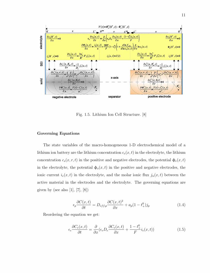
enough to incorporate further developments in a battery system. Fig. 1.5 shows the

Lithium Ion structure for the 1-D Model.

For analysis and control of lithium-ion batteries in hybrid environments (with a

fuel cell, capacitor, or electrical components), there is a need to simulate state of

charge, state of health, and other parameters of lithium-ion batteries in milliseconds.

Rigorous physics-based models take a few seconds up to a few minutes to simulate

discharge curves, depending on the solvers, routines, computers, etc. Circuit-based or

empirical models (based on the past data) can be simulated in milliseconds. However,

these models fail at various operating conditions, and use of these models might cause

abuse or under-utilization of electrochemical power sources. This paper presents

the mathematical analysis for reformulation of physics-based models and utilize this

models as baseline for the battery plant to further study the charging techniques.

11

Fig. 1.5. Lithium Ion Cell Structure. [8]

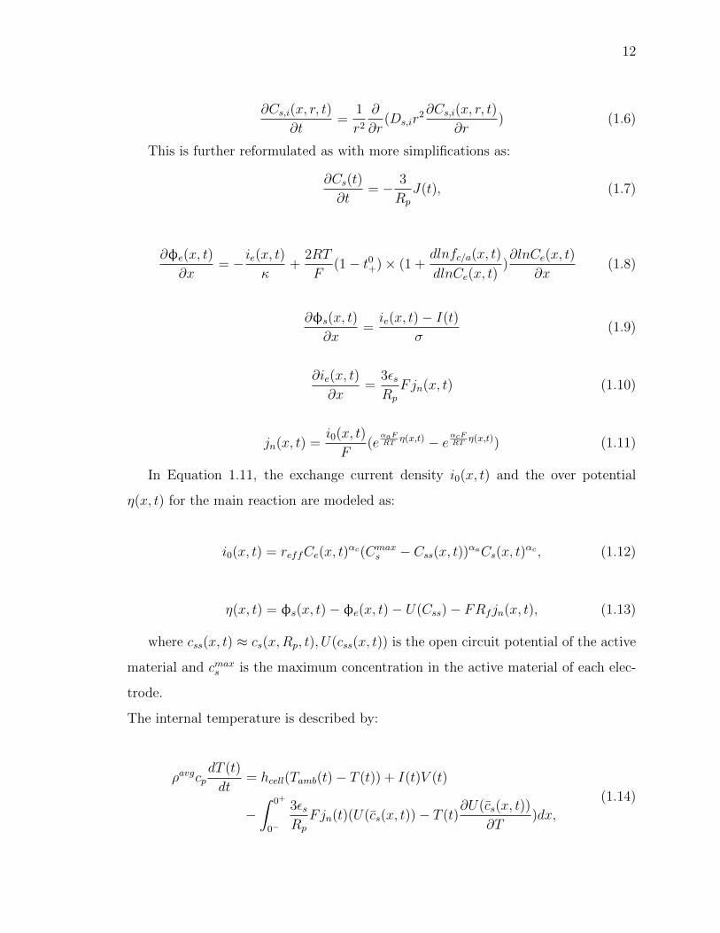
Governing Equations

The state variables of the macro-homogeneous 1-D electrochemical model of a

lithium ion battery are the lithium concentration ce(x, t) in the electrolyte, the lithium

concentration cs(x, r, t) in the positive and negative electrodes, the potential φe(x, t)

in the electrolyte, the potential φs(x, t) in the positive and negative electrodes, the

ionic current ie(x, t) in the electrolyte, and the molar ionic flux jn(x, t) between the

active material in the electrodes and the electrolyte. The governing equations are

given by (see also [1], [7], [8])

εp∂C(x, t)

∂t= Deff,p

∂C(x, t)2

∂x+ ap(1− t0+)jp (1.4)

Reordering the equation we get:

εe∂Ce(x, t)

∂t=

∂

∂x(εeDe

∂Ce(x, t)

∂x+

1− t0+F

ie(x, t)) (1.5)

12

∂Cs,i(x, r, t)

∂t=

1

r2

∂

∂r(Ds,ir

2∂Cs,i(x, r, t)

∂r) (1.6)

This is further reformulated as with more simplifications as:

∂Cs(t)

∂t= − 3

Rp

J(t), (1.7)

∂φe(x, t)

∂x= −ie(x, t)

κ+

2RT

F(1− t0+)× (1 +

dlnfc/a(x, t)

dlnCe(x, t))∂lnCe(x, t)

∂x(1.8)

∂φs(x, t)

∂x=ie(x, t)− I(t)

σ(1.9)

∂ie(x, t)

∂x=

3εsRp

Fjn(x, t) (1.10)

jn(x, t) =i0(x, t)

F(e

αaFRT

η(x,t) − eαcFRT

η(x,t)) (1.11)

In Equation 1.11, the exchange current density i0(x, t) and the over potential

η(x, t) for the main reaction are modeled as:

i0(x, t) = reffCe(x, t)αc(Cmax

s − Css(x, t))αaCs(x, t)αc , (1.12)

η(x, t) = φs(x, t)− φe(x, t)− U(Css)− FRfjn(x, t), (1.13)

where css(x, t) ≈ cs(x,Rp, t), U(css(x, t)) is the open circuit potential of the active

material and cmaxs is the maximum concentration in the active material of each elec-

trode.

The internal temperature is described by:

ρavgcpdT (t)

dt= hcell(Tamb(t)− T (t)) + I(t)V (t)

−∫ 0+

0−

3εsRp

Fjn(t)(U(cs(x, t))− T (t)∂U(cs(x, t))

∂T)dx,

(1.14)

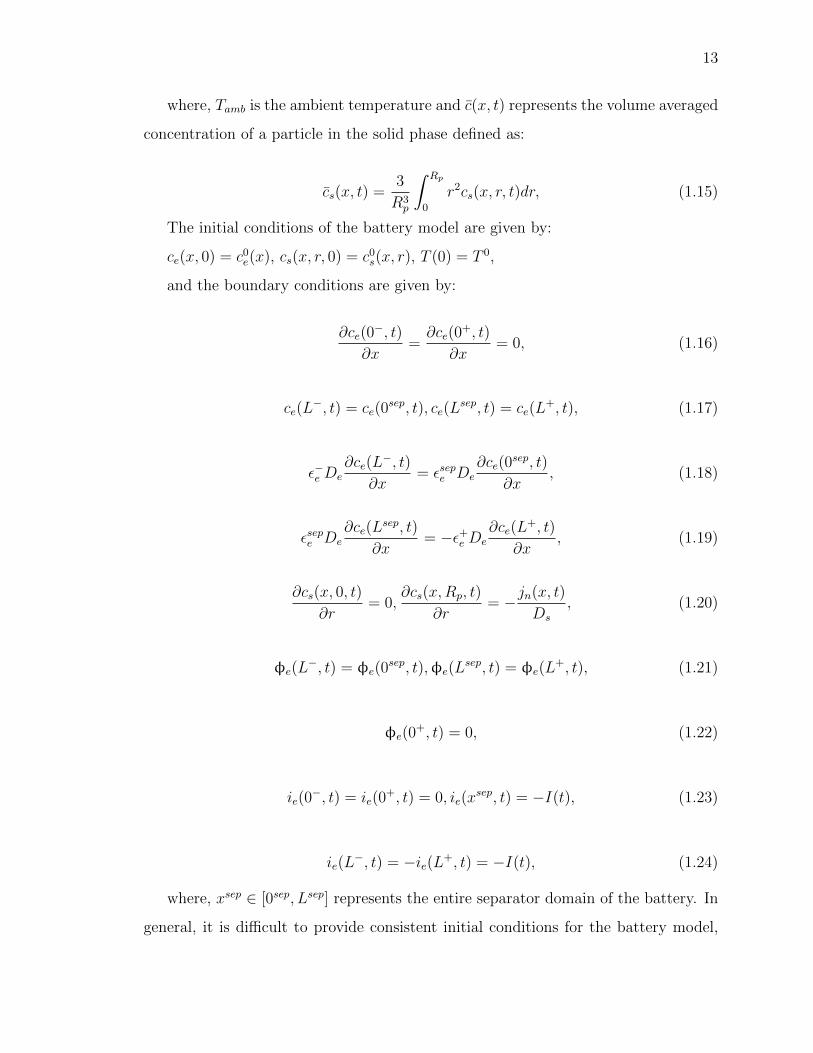
13

where, Tamb is the ambient temperature and c(x, t) represents the volume averaged

concentration of a particle in the solid phase defined as:

cs(x, t) =3

R3p

∫ Rp

0

r2cs(x, r, t)dr, (1.15)

The initial conditions of the battery model are given by:

ce(x, 0) = c0e(x), cs(x, r, 0) = c0

s(x, r), T (0) = T 0,

and the boundary conditions are given by:

∂ce(0−, t)

∂x=∂ce(0

+, t)

∂x= 0, (1.16)

ce(L−, t) = ce(0

sep, t), ce(Lsep, t) = ce(L

+, t), (1.17)

ε−e De∂ce(L

−, t)

∂x= εsepe De

∂ce(0sep, t)

∂x, (1.18)

εsepe De∂ce(L

sep, t)

∂x= −ε+e De

∂ce(L+, t)

∂x, (1.19)

∂cs(x, 0, t)

∂r= 0,

∂cs(x,Rp, t)

∂r= −jn(x, t)

Ds

, (1.20)

φe(L−, t) = φe(0

sep, t),φe(Lsep, t) = φe(L

+, t), (1.21)

φe(0+, t) = 0, (1.22)

ie(0−, t) = ie(0

+, t) = 0, ie(xsep, t) = −I(t), (1.23)

ie(L−, t) = −ie(L+, t) = −I(t), (1.24)

where, xsep ∈ [0sep, Lsep] represents the entire separator domain of the battery. In

general, it is difficult to provide consistent initial conditions for the battery model,

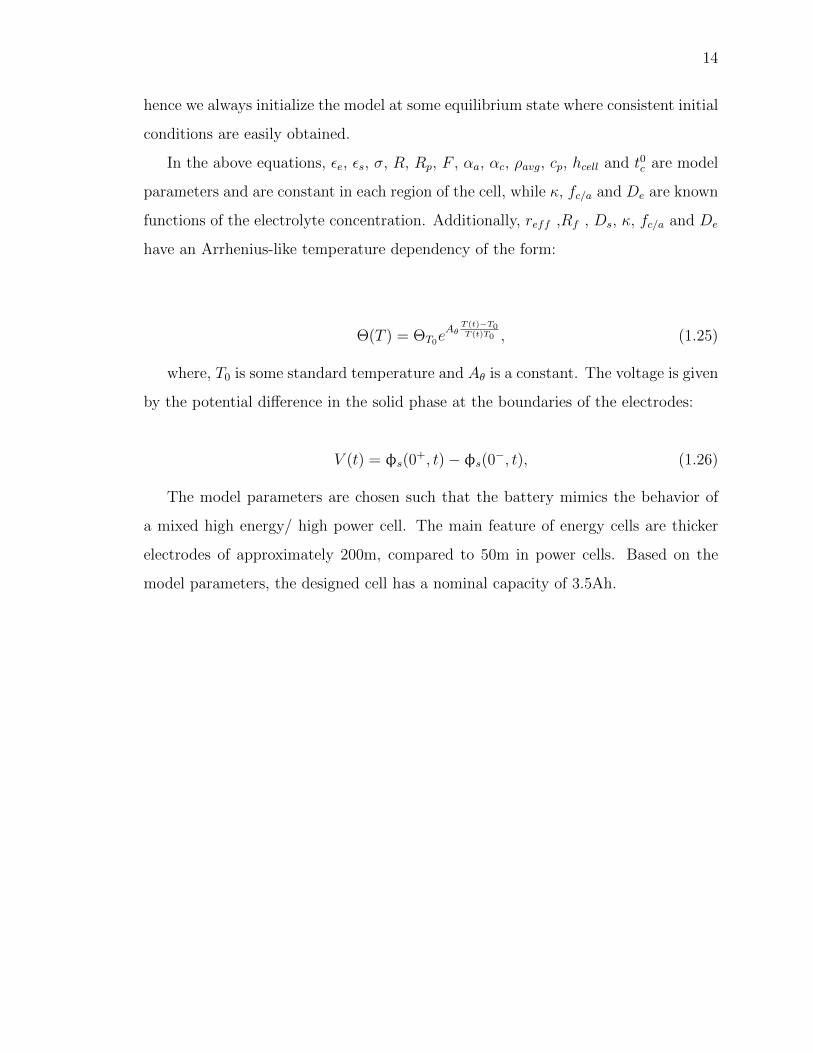
14

hence we always initialize the model at some equilibrium state where consistent initial

conditions are easily obtained.

In the above equations, εe, εs, σ, R, Rp, F , αa, αc, ρavg, cp, hcell and t0c are model

parameters and are constant in each region of the cell, while κ, fc/a and De are known

functions of the electrolyte concentration. Additionally, reff ,Rf , Ds, κ, fc/a and De

have an Arrhenius-like temperature dependency of the form:

Θ(T ) = ΘT0eAθ

T (t)−T0T (t)T0 , (1.25)

where, T0 is some standard temperature and Aθ is a constant. The voltage is given

by the potential difference in the solid phase at the boundaries of the electrodes:

V (t) = φs(0+, t)− φs(0

−, t), (1.26)

The model parameters are chosen such that the battery mimics the behavior of

a mixed high energy/ high power cell. The main feature of energy cells are thicker

electrodes of approximately 200m, compared to 50m in power cells. Based on the

model parameters, the designed cell has a nominal capacity of 3.5Ah.

15

2. LITERATURE SURVEY

2.1 Introduction

In this section a comparative study of the available techniques of charging a

Lithium-Ion battery is done. The Lithium-Ion charger is a voltage-limiting device

that is similar to the lead acid system. The difference lies in a higher voltage per

cell, tighter voltage tolerance and the absence of trickle or float charge at full charge.

While lead acid offers some flexibility in terms of voltage cutoff, manufacturers of

Lithium-Ion cells are very strict on the correct setting because Li-ion cannot accept

overcharge. The so-called miracle charger that promises to prolong battery life and

methods that pump extra capacity into the cell do not exist here. Li-ion is a clean

system and only takes what it can absorb. Anything extra causes stress. Most cells

charge to 4.20V/cell with a tolerance of +/50mV/cell. Higher voltages could increase

the capacity, but the resulting cell oxidation would reduce service life. More impor-

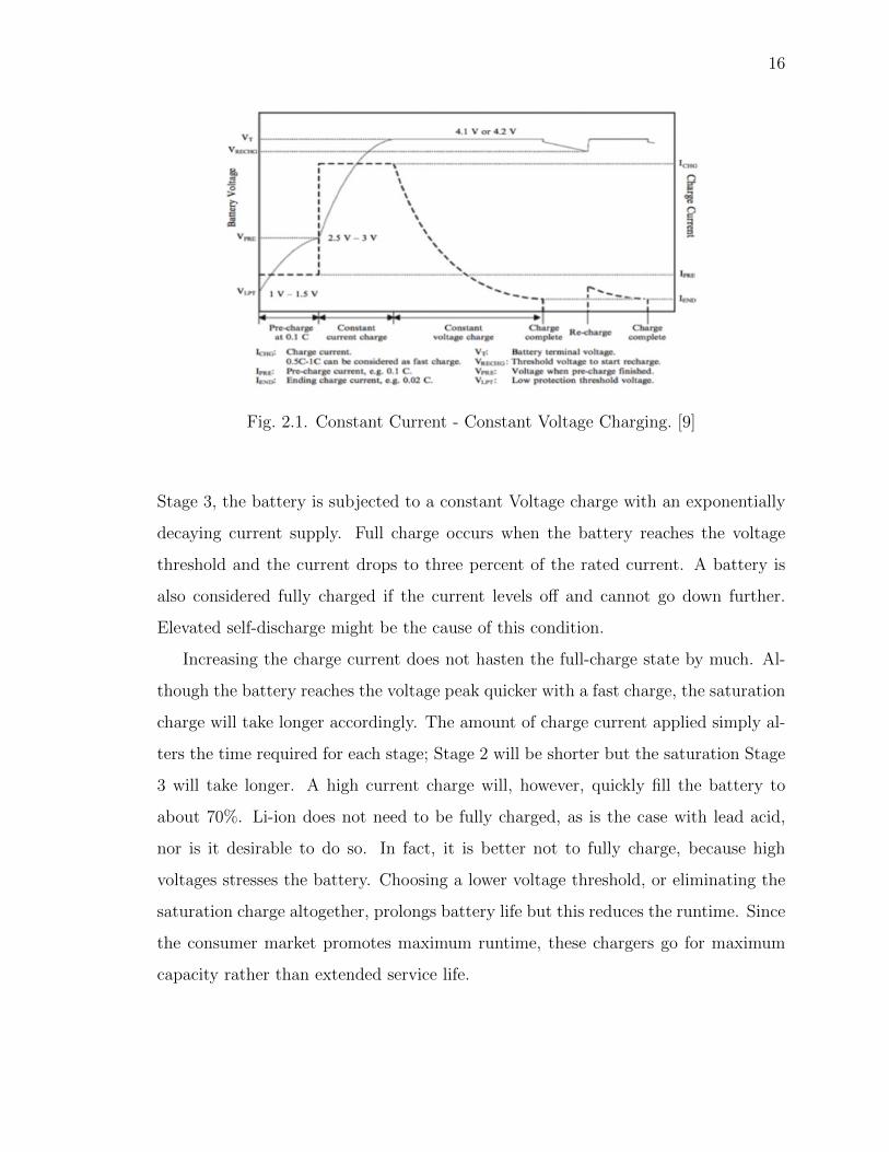
tant is the safety concern if charging beyond 4.20V/cell. Figure 1 shows the voltage

and current signature as lithium-ion passes through the stages for constant current

and topping charge.

The charge rate of a typical consumer Li-ion battery is between 0.5 and 1C in

Stage 2, which is the initial constant current charge stage, and the charge time is

about three hours. Usually the battery is not subjected to this current right from

the beginning of charging, which is Stage 1. In stage 1, a small current is supplied

to get the Lithium ions settle and adjust to the charging process. Manufacturers

recommend charging at 0.8C or less. Charge efficiency is 97 to 99 percent and the

cell remains cool during charge. Some Li-ion packs may experience a temperature

rise of about 5C (9F) when reaching full charge. This could be due to the protection

circuit and/or elevated internal resistance. After the constant current charge, at

16

Fig. 2.1. Constant Current - Constant Voltage Charging. [9]

Stage 3, the battery is subjected to a constant Voltage charge with an exponentially

decaying current supply. Full charge occurs when the battery reaches the voltage

threshold and the current drops to three percent of the rated current. A battery is

also considered fully charged if the current levels off and cannot go down further.

Elevated self-discharge might be the cause of this condition.

Increasing the charge current does not hasten the full-charge state by much. Al-

though the battery reaches the voltage peak quicker with a fast charge, the saturation

charge will take longer accordingly. The amount of charge current applied simply al-

ters the time required for each stage; Stage 2 will be shorter but the saturation Stage

3 will take longer. A high current charge will, however, quickly fill the battery to

about 70%. Li-ion does not need to be fully charged, as is the case with lead acid,

nor is it desirable to do so. In fact, it is better not to fully charge, because high

voltages stresses the battery. Choosing a lower voltage threshold, or eliminating the

saturation charge altogether, prolongs battery life but this reduces the runtime. Since

the consumer market promotes maximum runtime, these chargers go for maximum

capacity rather than extended service life.

17

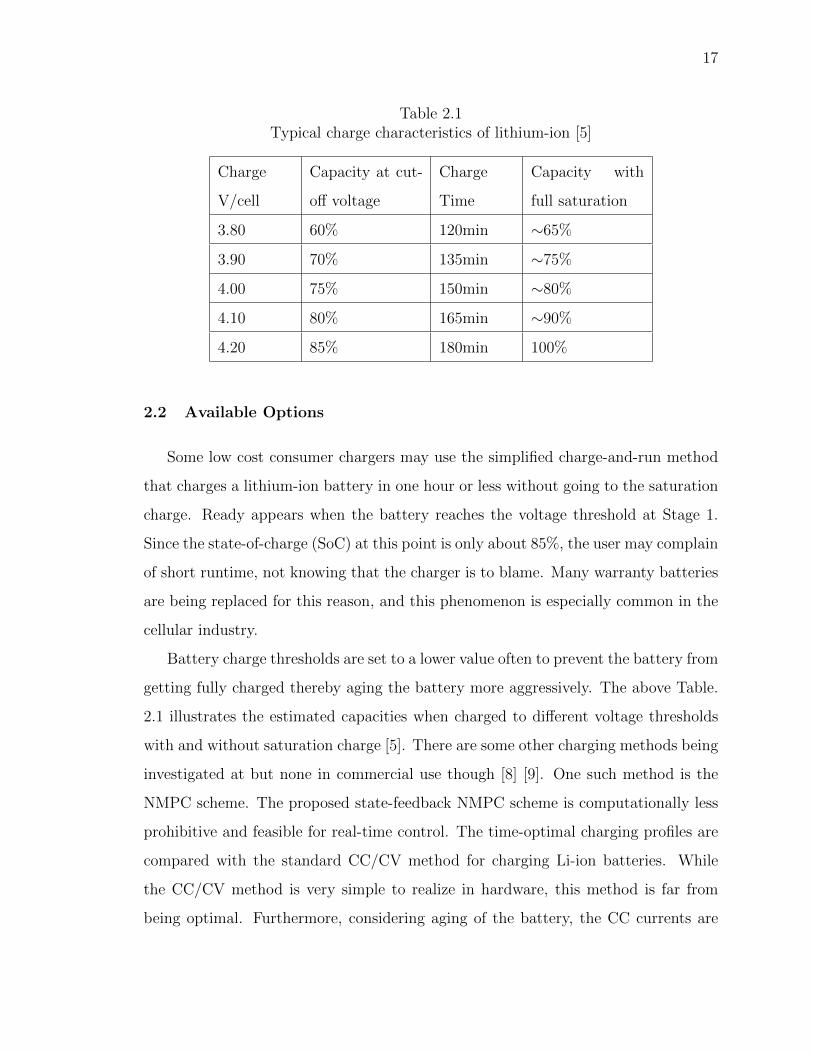
Table 2.1Typical charge characteristics of lithium-ion [5]

Charge

V/cell

Capacity at cut-

off voltage

Charge

Time

Capacity with

full saturation

3.80 60% 120min ∼65%

3.90 70% 135min ∼75%

4.00 75% 150min ∼80%

4.10 80% 165min ∼90%

4.20 85% 180min 100%

2.2 Available Options

Some low cost consumer chargers may use the simplified charge-and-run method

that charges a lithium-ion battery in one hour or less without going to the saturation

charge. Ready appears when the battery reaches the voltage threshold at Stage 1.

Since the state-of-charge (SoC) at this point is only about 85%, the user may complain

of short runtime, not knowing that the charger is to blame. Many warranty batteries

are being replaced for this reason, and this phenomenon is especially common in the

cellular industry.

Battery charge thresholds are set to a lower value often to prevent the battery from

getting fully charged thereby aging the battery more aggressively. The above Table.

2.1 illustrates the estimated capacities when charged to different voltage thresholds

with and without saturation charge [5]. There are some other charging methods being

investigated at but none in commercial use though [8] [9]. One such method is the

NMPC scheme. The proposed state-feedback NMPC scheme is computationally less

prohibitive and feasible for real-time control. The time-optimal charging profiles are

compared with the standard CC/CV method for charging Li-ion batteries. While

the CC/CV method is very simple to realize in hardware, this method is far from

being optimal. Furthermore, considering aging of the battery, the CC currents are

18

in general chosen very conservative, such that safety can be guaranteed during the

lifetime of the battery.

19

3. METHODOLOGY

3.1 Introduction

Lithium Ion battery can be modeled in a variety of techniques. Equivalent Circuit

Model, 1-D Electrochemical Model, 2-D Electrochemical Model, Multi Dimensional -

Multi Particle Model are some of the techniques used to model the Battery Dynam-

ics. No one model can be used to suffice the need of different applications. Some

model provide higher computational speed where some other provide more accurate

performance. The choice of a particular model depends on the usage and the require-

ments. Like, R-C models are simple and computationally fast but lag the accurate

performance required for a charge/discharge characterization study. On the contrary

a full order multi dimensional, multi particle model is accurate to the level of details

but is super slow for ordinary application needs. Hence the choice of a model requires

good amount of insight into the requirements and application it will be used at. If a

high speed medium accurate model is good enough for a particular application then

that is the best choice.

3.2 Cell Model

One of the primary objective of designing an optimal control for Lithium Ion

battery is the creation of a robust, high fidelity battery plant model. Generally, the

effort of developing a detailed multi-scale and multi-physics model with high predic-

tive ability is very expensive, so model development efforts begin with a simple model

and then add more physics until the model predictions are sufficiently accurate.That

is, model development starts from the simplest form and increases in complexity un-

til the satisfying performance is achieved as per the objective and requirement. The

20

best possible physics-based model can depend on the type of issue being addressed,

the systems requirement objectives and accuracy desired and on the available com-

putational resources. This section describes various types of models available in the

literature, the modeling efforts being undertaken so far and the difficulties in using

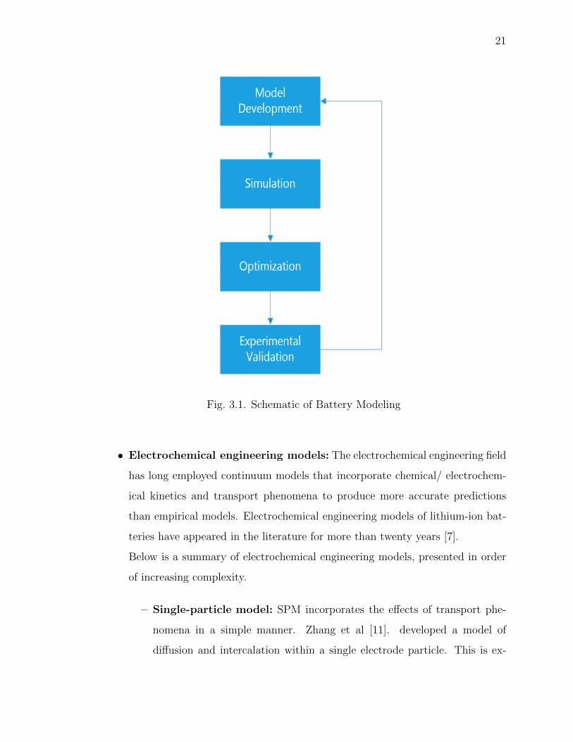
the most comprehensive models in all scenarios. Fig. 3.1 shows the basic approach

in designing a system for a battery model.

An important task is to experimentally validate the chosen model to ensure that

the model predicts the experimental data to the required precision with a reasonable

confidence. This task is typically performed in part for experiments designed to

evaluate the descriptions of physio-chemical phenomena in the model whose validity

is less well established. However, in a materials system such as a lithium-ion battery,

most variables in the system are not directly measurable during charge-discharge

cycles, and hence are not available for comparison to the corresponding variables

in the model to fully verify the accuracy of all of the physio-chemical assumptions

made in the derivation of the model. Also, model parameters that cannot be directly

measured experimentally typically have to be obtained by comparing the experimental

data with the model predictions.

Models for the prediction of battery performance can be roughly grouped into

four categories: empirical models, electrochemical engineering models, multi-physics

models, and molecular/atomic models [10].

• Empirical models: Empirical models employ past experimental data to pre-

dict the future behavior of lithium-ion batteries without consideration of physio-

chemical principles. Polynomial, exponential, power law, logarithmic, and trigono-

metric functions are commonly used as empirical models. The computational

simplicity of empirical models enables very fast computations, but since these

models are based on fitting experimental data for a specific set of operating

conditions, predictions can be very poor for other battery operating

21

Fig. 3.1. Schematic of Battery Modeling

• Electrochemical engineering models: The electrochemical engineering field

has long employed continuum models that incorporate chemical/ electrochem-

ical kinetics and transport phenomena to produce more accurate predictions

than empirical models. Electrochemical engineering models of lithium-ion bat-

teries have appeared in the literature for more than twenty years [7].

Below is a summary of electrochemical engineering models, presented in order

of increasing complexity.

– Single-particle model: SPM incorporates the effects of transport phe-

nomena in a simple manner. Zhang et al [11]. developed a model of

diffusion and intercalation within a single electrode particle. This is ex-

22

panded to a sandwich model by considering the anode and cathode each as

a single particle with the same surface area as the electrode [12]. Diffusion

and intercalation are considered within the particle in this model. Con-

centration and potential effects in the solution phase between the particles

are neglected

– Ohmic porous-electrode models: Next in complexity order, porous elec-

trode model is studied. This model uses the solid and electrolyte phase

potentials and current but neglect the spatial variation in the concentra-

tions. The model assumes either linear, Tafel or exponential kinetics for

the electrochemical reactions and incorporates some additional phenom-

ena, such as the dependency on conductivity as a function of porosity.

Optimization studies have been performed using this model to design the

separator and electrode thicknesses [13], [14] and ideal spatial variations

of porosity within electrodes.

– Pseudo-two-dimensional models: The pseudo-two-dimensional (P2D)

model expands on the ohmic porous-electrode model by including diffusion

in the electrolyte and solid phases, as well as Butler-Volmer kinetics (1.5).

Doyle et al [7]. developed a P2D model based on concentrated solution

theory to describe the internal behavior of a lithium-ion sandwich consist-

ing of positive and negative porous electrodes, a separator, and a current

collector. This model was generic enough to incorporate further advance-

ments in battery systems understanding, leading to the development of a

number of similar models [12], [15–25]. This physics-based model is by

far the most used by battery researchers, and solves for the electrolyte

concentration, electrolyte potential, solid-state potential, and solid-state

concentration within the porous electrodes and the electrolyte concentra-

tion and electrolyte potential within the separator

23

• Multiphysics models: Multi-scale, multidimensional, and multi-physics elec-

trochemical, thermal coupled models are necessary to accurately describe all

of the important phenomena that occur during the operation of lithium-ion

batteries for high power/energy applications such as in electric/hybrid vehicles.

– Thermal models: Including temperature effects into the P2D model adds

to the complexity, but also to the validity, of the model, especially in high

power/energy applications. Due to the added computational load required

to perform thermal calculations, many researchers have decoupled the ther-

mal equations from the electrochemical equations by using a global energy

balance, which makes it impossible to monitor the effects on the perfor-

mance of the cells due to temperature changes [26–30]. Other researchers

have similarly decoupled the thermal simulation of the battery stack from

the thermal/electrochemical simulation of a single cell sandwich [31,32].

– Stack models: In order to simulate battery operation more accurately,

battery models are improved by considering multiple cells arranged in a

stack configuration. Simulation of the entire stack is important when ther-

mal or other effects cause the individual cells to operate differently from

each other. Since it is often not practical or possible to measure each cell

individually in a stack, these differences can lead to potentially dangerous

or damaging conditions such as overcharging or deep-discharging certain

cells within the battery, which can cause thermal runaway or explosions.

• Molecular/atomistic models: Kinetic Monte Carlo method :- The Kinetic

Monte Carlo (KMC) method is a stochastic approach that has been used to

model the discharge behavior of lithium ions during intercalation. Such models

[33–36] have been used to simulate diffusion of lithium from site to site within

an active particle to aid in understanding on how different crystal structures

affect lithium mobility [37] and how the activation barrier varies with lithium-

ion concentration [35,36]. Additionally, Monte Carlo methods have been used to

24

predict thermodynamic properties [38]. KMC has also been applied to simulate

the growth of the passive SEI-layer across the surface of the electrode particle,

to simulate one of the mechanisms for capacity fade

In this work, a reformulated 1-D electrochemical model is used which is computa-

tionally fast as well as accurate to the level of details required for the work. A brief

overview of the RC Model is given in the below section and a detailed analysis of the

physics based electrochemical model is presented in the following subsections.

3.2.1 Equivalent Circuit Model

The Battery cell can be modeled as a simplistic RC model. The RC model is

good enough in many applications but not very accurate and detailed to the level

this literature requires. Various equivalent circuit models such as the Rint model,

the RC model, the Thevenin model or the PNGV model are now widely used

in Electric Vehicle studies. In order to refine the polarization characteristics of a

battery, an improved Thevenin circuit model named DP (for dual polarization) model

is proposed herein. Further, comparisons between the model-based simulation data

and the experimental data are carried out to evaluate the validity of the foregoing

models, which provides a foundation for the model-based SOC estimation.

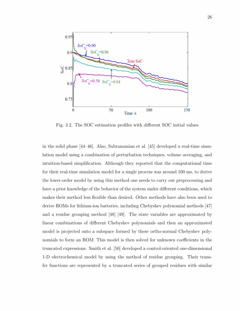
The below Fig. 3.2, shows the SOC estimate by the different Equivalent Circuit

Models

3.2.2 Physics Based Cell Model

Doyle et al. and Fuller et al. [7] published a physics-based model for a lithium-ion

cell, which has been used or modified by others [39–43]. These models are com-

putationally very expensive to be considered as a potential optimal candidate for

battery simulations. Consequently, several simplifications of their model have been

published to reduce the computation time associated with diffusion of lithium ions

25

Tab

le3.

1T

he

stat

isti

cal

anal

ysi

sof

the

abso

lute

valu

esof

term

inal

volt

age

erro

rs

Model

Maximum

(V)

Mean

(V)

Variance

(V2)

Max.ErrorRate

(%)

RintM

odel

1.62

290.

3945

0.07

622.

8176

RCModel

1.07

850.

2336

0.04

632.

0337

TheveninModel

0.29

670.

0455

0.02

200.

5151

PNGVModel

0.57

720.

0875

0.02

431.

0020

DPModel

0.21

830.

0429

0.00

210.

3790

26

Fig. 3.2. The SOC estimation profiles with different SOC initial values

in the solid phase [44–46]. Also, Subramanian et al. [45] developed a real-time simu-

lation model using a combination of perturbation techniques, volume averaging, and

intuition-based simplification. Although they reported that the computational time

for their real-time simulation model for a single process was around 100 ms, to derive

the lower-order model by using this method one needs to carry out preprocessing and

have a prior knowledge of the behavior of the system under different conditions, which

makes their method less flexible than desired. Other methods have also been used to

derive ROMs for lithium-ion batteries, including Chebyshev polynomial methods [47]

and a residue grouping method [48] [49]. The state variables are approximated by

linear combinations of different Chebyshev polynomials and then an approximated

model is projected onto a subspace formed by these ortho-normal Chebyshev poly-

nomials to form an ROM. This model is then solved for unknown coefficients in the

truncated expressions. Smith et al. [50] developed a control-oriented one-dimensional

1-D electrochemical model by using the method of residue grouping. Their trans-

fer functions are represented by a truncated series of grouped residues with similar

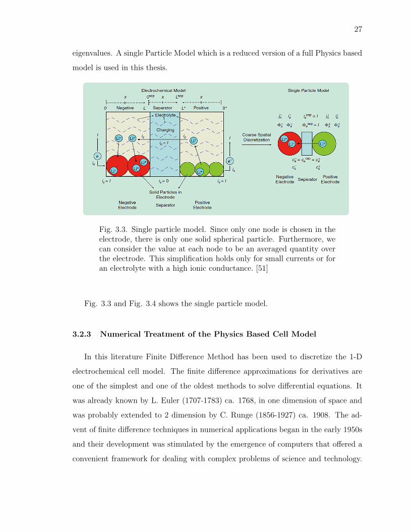
27

eigenvalues. A single Particle Model which is a reduced version of a full Physics based

model is used in this thesis.

Fig. 3.3. Single particle model. Since only one node is chosen in theelectrode, there is only one solid spherical particle. Furthermore, wecan consider the value at each node to be an averaged quantity overthe electrode. This simplification holds only for small currents or foran electrolyte with a high ionic conductance. [51]

Fig. 3.3 and Fig. 3.4 shows the single particle model.

3.2.3 Numerical Treatment of the Physics Based Cell Model

In this literature Finite Difference Method has been used to discretize the 1-D

electrochemical cell model. The finite difference approximations for derivatives are

one of the simplest and one of the oldest methods to solve differential equations. It

was already known by L. Euler (1707-1783) ca. 1768, in one dimension of space and

was probably extended to 2 dimension by C. Runge (1856-1927) ca. 1908. The ad-

vent of finite difference techniques in numerical applications began in the early 1950s

and their development was stimulated by the emergence of computers that offered a

convenient framework for dealing with complex problems of science and technology.

28

Fig. 3.4. Single particle model detailed structure. [51]

Theoretical results have been obtained during the last five decades regarding the ac-

curacy, stability and convergence of the finite difference method for partial differential

equations. In this work the reformulated battery governing equations are discretized

at their time and space grid points using FDM. The Equations are then solved for

their value at the next grid point. While solving the equations for the grid points the

boundary and initial values are applied to maintain the equation limits. This process

is followed until a convergence is reached with a given degree of accuracy.

29

Finite difference approximations

The principle of FDM is very similar to numerical methods used to solve ODEs. In

this method the differential operator is approximated by replacing it with the deriva-

tives in the equation using differential quotients. The solution domain is divided into

space and time nodes and the differentiation is approximated at each node. The

difference between the solved numerical solution and the exact analytical solution is

determined by the error that is committed by going from a differential operator to

a difference operator. This error is called the quantization error or truncation error.

The truncation error proves the fact that a finite part of the Taylor series is used in

the approximation.

Here we have considered one-dimensional space only for simplicity. The main

concept behind any finite difference scheme is related to the definition of the derivative

of a smooth function u at a point x ∈ R :

u′(x) = limh→0

u(x+ h)− u(x)

h,

and, to the fact that when h tends to 0 (without vanishing), the quotient on the

right-hand side provides a good approximation of the derivative. In other words, h

should be sufficiently small to get a good approximation. It remains to indicate what

exactly is a good approximation, in what sense. Actually, the approximation is good

when the error committed in this approximation (i.e. when replacing the derivative

by the differential quotient) tends towards zero when h tends to zero. If the function

u is sufficiently smooth in the neighborhood of x, it is possible to quantify this error

using a Taylor expansion.

Finite Difference Method

1D : Ω = (0, X), ui ≈ u(xi), i = 0 , 1 , . . . ,N

30

grid points : xi = i∆x mesh size : ∆x =X

N

First-Order derivatives:

∂u

∂x(x) = lim

∆x→0

u(x+ ∆x)− u(x)

∆x= lim

∆x→0

u(x)− u(x−∆x)

∆x

= lim∆x→0

u(x+ ∆x)− u(x−∆x)

∆x,

(3.1)

The first order derivatives are approximated in the following 3 ways.

• Forward difference:

(∂u

∂x)i ≈

ui+1 − ui∆x

(3.2)

• Backward difference:

(∂u

∂x)i ≈

ui − ui−1

∆x(3.3)

• Central difference:

(∂u

∂x)i ≈

ui+1 − ui−1

2∆x(3.4)

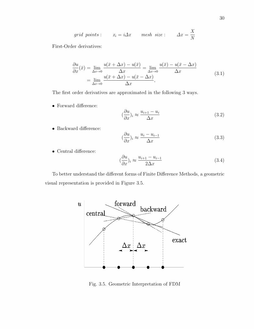
To better understand the different forms of Finite Difference Methods, a geometric

visual representation is provided in Figure 3.5.

Fig. 3.5. Geometric Interpretation of FDM

31

Taylor series expansion u(x) =∞∑n=0

(x−xi)nn!

(∂nu∂xn

)i, u ∈ C∞([0, X])

T1 : ui+1 = ui + ∆x(∂u∂x

)i + (∆x)2

2(∂

2u∂x2

)i + (∆x)3

6(∂

3u∂x3

)i + . . .

T2 : ui−1 = ui −∆x(∂u∂x

)i + (∆x)2

2(∂

2u∂x2

)i − (∆x)3

6(∂

3u∂x3

)i + . . .

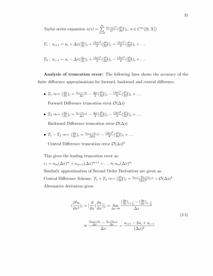
Analysis of truncation error: The following lines shows the accuracy of the

finite difference approximations for forward, backward and central difference.

• T1 ⇒= (∂u∂x

)i = ui+1−ui∆x

− ∆x2

(∂2u∂x2

)i − (∆x)2

6(∂

3u∂x3

)i + . . .

Forward Difference truncation error O(∆x)

• T2 ⇒= (∂u∂x

)i = ui−ui−1

∆x− ∆x

2(∂

2u∂x2

)i − (∆x)2

6(∂

3u∂x3

)i + . . .

Backward Difference truncation error O(∆x)

• T1 − T2 ⇒= (∂u∂x

)i = ui+1−ui−1

∆2x− (∆x)2

6(∂

3u∂x3

)i + . . .

Central Difference truncation error O(∆x)2

This gives the leading truncation error as:

ετ = αm(∆x)m + αm+1(∆x)m+1 + . . . ≈ αm(∆x)m

Similarly approximation of Second Order Derivatives are given as:

Central Difference Scheme: T1 + T2 ⇒= (∂2u∂x2

)i = ui+1−2ui+ui−1

(∆x)2+O(∆x)2

Alternative derivation gives:

(∂2u

∂x2)i = [

∂

∂x(∂u

∂x)]i = lim

∆x→0

(∂u∂x

)i+ 12− (∂u

∂x)i− 1

2

∆x

≈ui+1−ui

∆x− ui−ui−1

∆x

∆x=ui+1 − 2ui + ui−1

(∆x)2

(3.5)

32

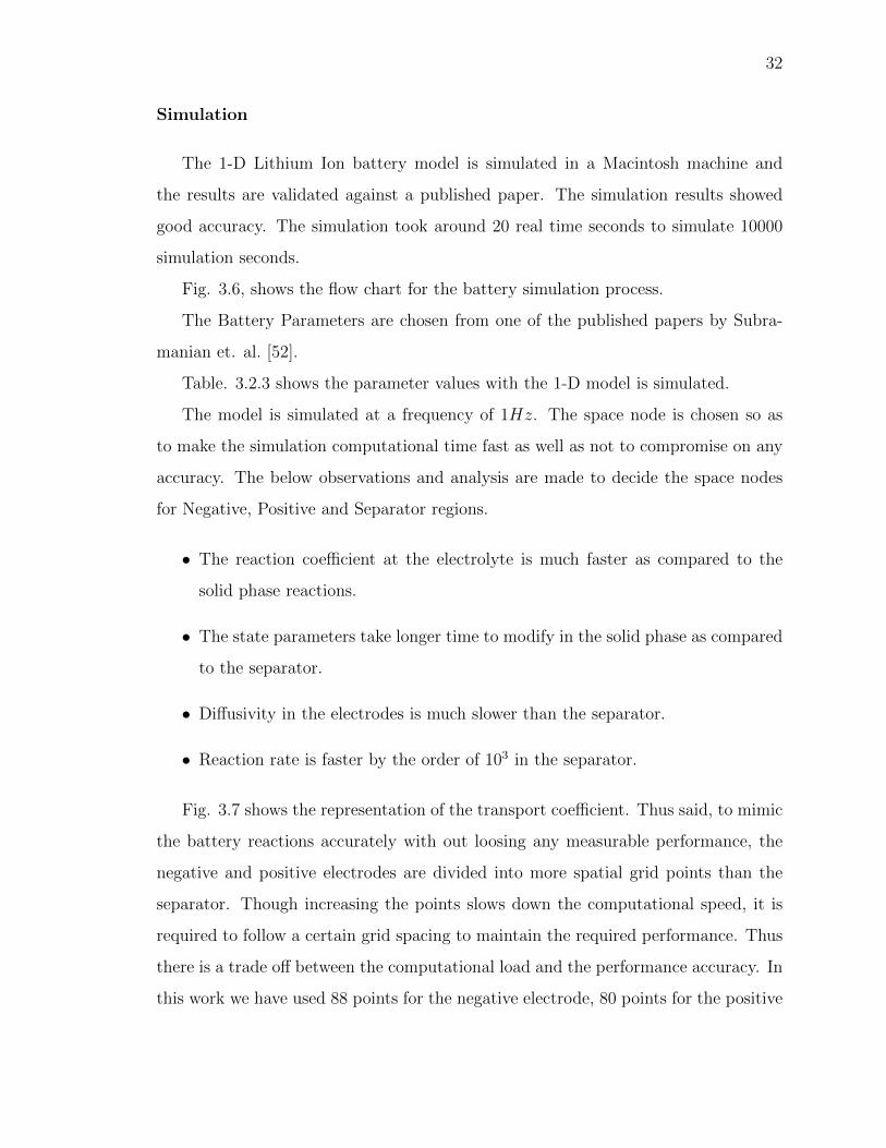
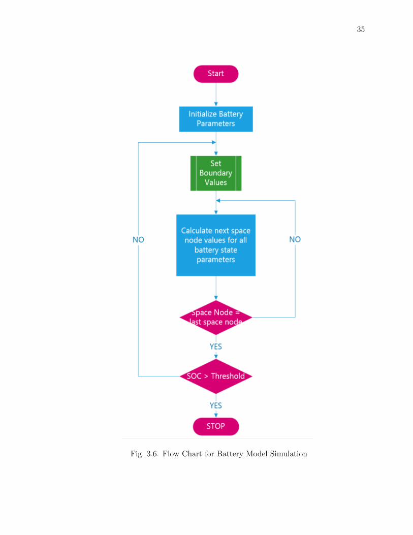
Simulation

The 1-D Lithium Ion battery model is simulated in a Macintosh machine and

the results are validated against a published paper. The simulation results showed

good accuracy. The simulation took around 20 real time seconds to simulate 10000

simulation seconds.

Fig. 3.6, shows the flow chart for the battery simulation process.

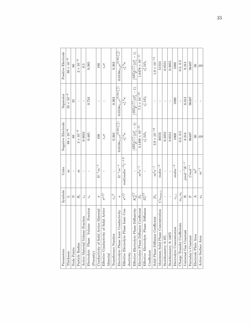
The Battery Parameters are chosen from one of the published papers by Subra-

manian et. al. [52].

Table. 3.2.3 shows the parameter values with the 1-D model is simulated.

The model is simulated at a frequency of 1Hz. The space node is chosen so as

to make the simulation computational time fast as well as not to compromise on any

accuracy. The below observations and analysis are made to decide the space nodes

for Negative, Positive and Separator regions.

• The reaction coefficient at the electrolyte is much faster as compared to the

solid phase reactions.

• The state parameters take longer time to modify in the solid phase as compared

to the separator.

• Diffusivity in the electrodes is much slower than the separator.

• Reaction rate is faster by the order of 103 in the separator.

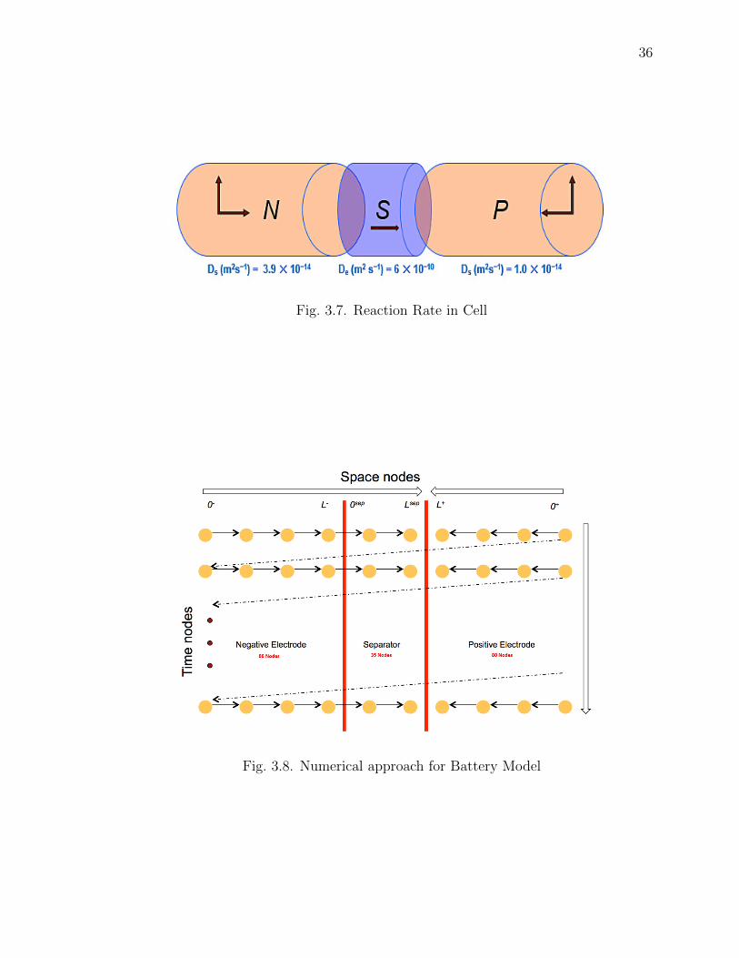
Fig. 3.7 shows the representation of the transport coefficient. Thus said, to mimic

the battery reactions accurately with out loosing any measurable performance, the

negative and positive electrodes are divided into more spatial grid points than the

separator. Though increasing the points slows down the computational speed, it is

required to follow a certain grid spacing to maintain the required performance. Thus

there is a trade off between the computational load and the performance accuracy. In

this work we have used 88 points for the negative electrode, 80 points for the positive

33

Para

met

ers

Sym

bols

Un

its

Neg

ati

ve

Ele

ctro

de

Sep

ara

tor

Posi

tive

Ele

ctro

de

Th

ickn

ess

Lm

88×

10−6

35×

10−6

80×

10−6

Nod

eP

oin

tsN

-88

35

80

Part

icle

Rad

ius

Ri

m2×

10−6

-2×

10−6

Act

ive

Mate

rial

Volu

me

Fra

ctio

nε s

-0.4

824

-0.5

Ele

ctro

lyte

Ph

ase

Volu

me

Fra

ctio

n

(Poro

sity

)

ε e-

0.4

85

0.7

24

0.3

85

Con

du

ctiv

ity

of

Solid

Act

ive

Mate

rial

σΩ

−1m

−1

100

-100

Eff

ecti

ve

Con

du

ctiv

ity

of

Solid

Act

ive

Mate

rial

σeff

-ε sσ

-ε sσ

Tra

nsf

eren

ceN

um

ber

t +0

-0.3

63

0.3

63

0.3

63

Ele

ctro

lyte

Ph

ase

Ion

icC

on

du

ctiv

ity

κΩ

−1m

−1

0.0

158c e,ne(

0.85c1.4

e,n

)0.0

158c e,se(

0.85c1.4

e,s

)0.0

158c e,pe(

0.85c1.4

e,p

)

Eff

ecti

ve

Ele

ctro

lyte

Ph

ase

Ion

icC

on

-

du

ctiv

ity

κeff

mol(molm

−3)−

1.5

ε1.5eκ

ε1.5eκ

ε1.5eκ

Eff

ecti

ve

Ele

ctro

lyte

Ph

ase

Diff

usi

vit

yKeff

D-

[2RTκeff

F](t0 +−

1)

[2RTκeff

F](t0 +−

1)

[2RTκeff

F](t0 +−

1)

Ele

ctro

lyte

Ph

ase

Diff

usi

on

Coeffi

cien

tDe

m2s−

14.1

498×

10−11

7.5×

10−10

1.6

478×

10−11

Eff

ecti

ve

Ele

ctro

lyte

Ph

ase

Diff

usi

on

Coeffi

cien

t

Deff

e-

ε1 e.5De

ε1 e.5De

ε1 e.5De

Solid

Ph

ase

Diff

usi

on

Coeffi

cien

tDs

m2s−

13.9×

10−14

-1.0×

10−14

Maxim

um

Solid

Ph

ase

Con

centr

ati

on

Cs m

ax,i

molm

−3

30555

-51554

Sto

ich

iom

etry

@0%

--

0.4

955

-0.8

551

Sto

ich

iom

etry

@100%

--

0.8

551

-0.4

955

Ele

ctro

lyte

Con

centr

ati

on

c e,i

molm

−3

1000

1000

1000

Ch

arg

eT

ran

sfer

Coeffi

cien

tsαa,αc

-0.5

,0.5

-0.5

,0.5

Un

iver

sal

Gas

Con

stant

Rjm

ol−

1K

−1

8.3

14

8.3

14

8.3

14

Farr

ad

ay’s

Con

stant

FCmol−

196487

96487

96487

Ele

ctro

de

Pla

teA

rea

Am

230

-30

Act

ive

Su

rface

Are

aas

m−1

3εR

-3εR

34

electrode and 35 points for the separator, when using the 1-D model with constant

electrolyte concentration. When using modeled electrolyte concentration (where the

physics based model of Ce is used), we used a generic 10 point grids for Negative,

Positive and separator region. The performance is verified from the simulation results.

A simplistic way of describing the FDM approach to numerically solve the 1-D model

is presented below, in Fig. 3.8.

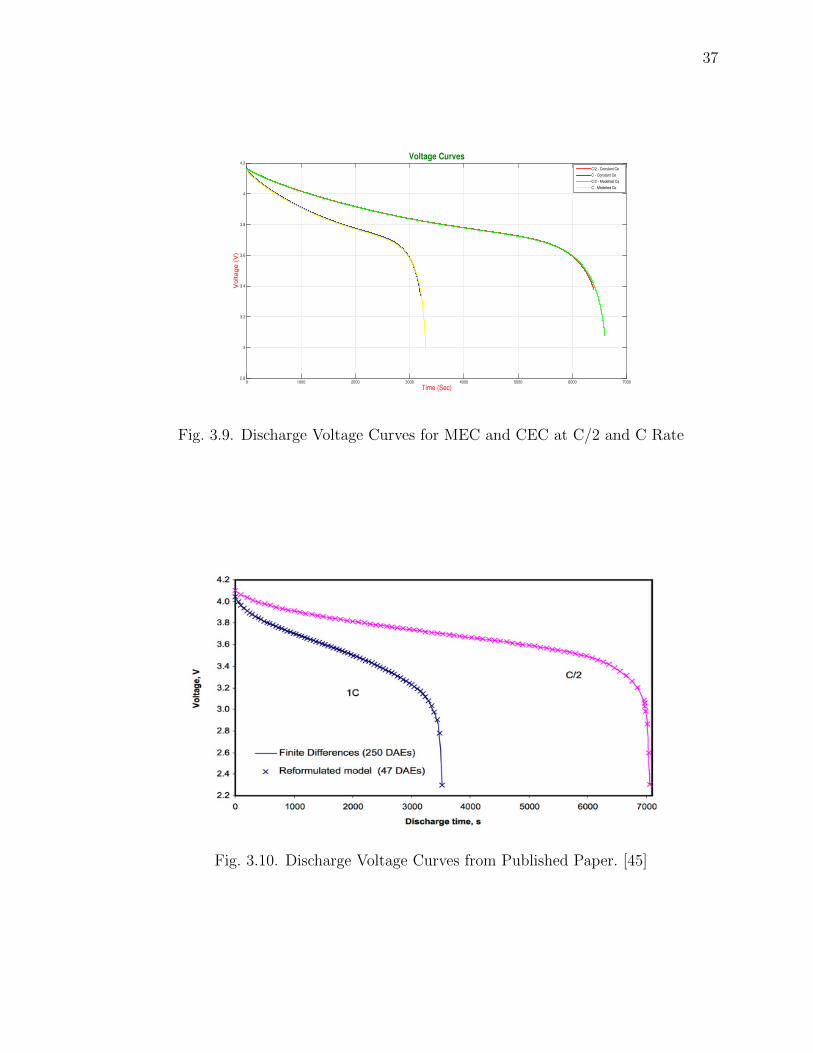
Model Validation Plots

The plant model is validated against a published paper by Subramanian et. al. [52]

The 1-D Model is also verified with MEC.

Fig. 3.9 and Fig.3.10 shows the discharge curves for CEC as well as MEC for C/2

and C discharge rates. The subsequent plot shows the discharge voltage curves from

the published paper.

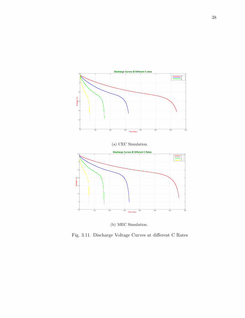
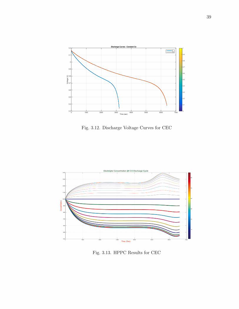
Fig. 3.11 and Fig. 3.12 shows the Discharge Voltage Curves at different C rates

for CEC and MEC.

Fig. 3.13, shows the electrolyte concentration for MEC Battery Model Sim-

ulation. Electrolyte concentration starts from the constant initial value and de-

creases/increases on the positive/negative electrode with time and space nodes.

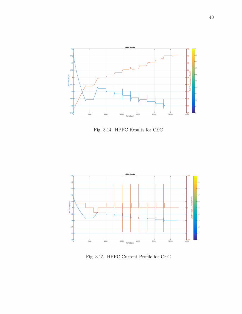
Fig. 3.14 and Fig. 3.15 shows the HPPC Voltage profiles with temperature

and current. In this cycle the battery is simulated with alternating charge and dis-

charge cycles with Pulsed regeneration/load currents. The battery voltage shows a

charge/discharge trend whereas the temperature shows a gradual increasing trend.

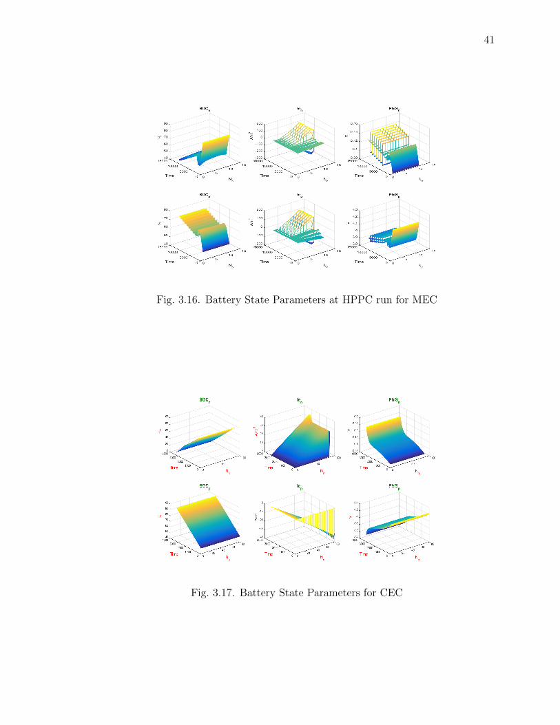
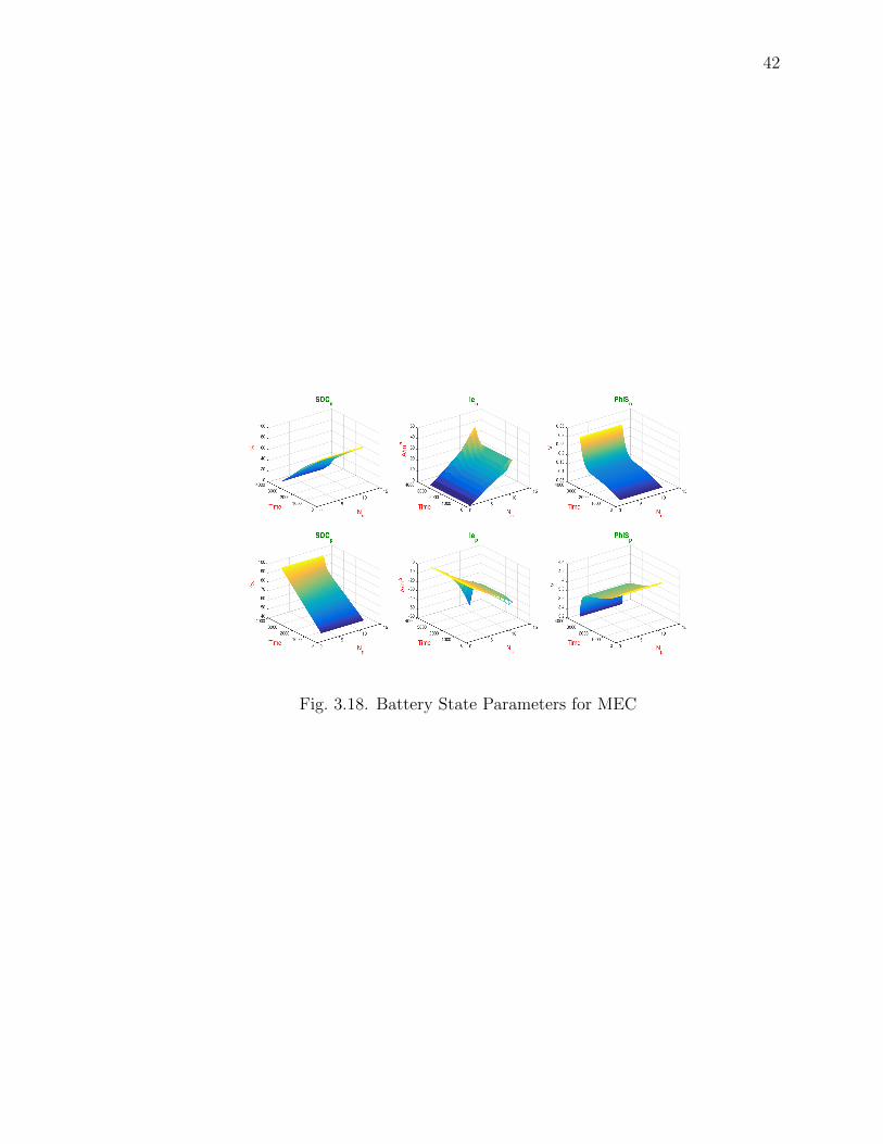
Fig. 3.17 and Fig. 3.18, Fig. 3.16 shows the Battery state parameters for CEC

and MEC simulations at 1C discharge rate.

35

Fig. 3.6. Flow Chart for Battery Model Simulation

36

Fig. 3.7. Reaction Rate in Cell

Fig. 3.8. Numerical approach for Battery Model

37

Time (Sec)0 1000 2000 3000 4000 5000 6000 7000

Voltage (

V)

2.8

3

3.2

3.4

3.6

3.8

4

4.2Voltage Curves

C/2 - Constant Ce

C - Constant Ce

C/2 - Modelled Ce

C - Modelled Ce

Fig. 3.9. Discharge Voltage Curves for MEC and CEC at C/2 and C Rate

Fig. 3.10. Discharge Voltage Curves from Published Paper. [45]

38

Time (Sec)0 1000 2000 3000 4000 5000 6000 7000

Vo

lta

ge

(V

)

3

3.2

3.4

3.6

3.8

4

4.2Discharge Curves @ Different C rates

C/2C2C5C

(a) CEC Simulation.

Time (Sec)0 1000 2000 3000 4000 5000 6000 7000

Vo

lta

ge

(V

)

2.8

3

3.2

3.4

3.6

3.8

4

4.2Discharge Curves @ Different C Rates

C/2

C

2C

5C

(b) MEC Simulation.

Fig. 3.11. Discharge Voltage Curves at different C Rates

39

Time (sec)0 1000 2000 3000 4000 5000 6000 7000

Vo

lta

ge

(V

)

3.3

3.4

3.5

3.6

3.7

3.8

3.9

4

4.1

4.2Discharge Curves - Constant Ce

0

0.1

0.2

0.3

0.4

0.5

0.6

0.7

0.8

0.9

1

CC/2

Fig. 3.12. Discharge Voltage Curves for CEC

Fig. 3.13. HPPC Results for CEC

40

Time (sec)0 2000 4000 6000 8000 10000 12000 14000

Ce

ll V

olta

ge

(V

)

3.75

3.8

3.85

3.9

3.95

4

4.05

4.1

4.15

4.2HPPC Profile

Ce

ll T

em

pe

ratu

re (

De

gC

)

24

26

28

30

32

34

36

38

40

42

0

0.1

0.2

0.3

0.4

0.5

0.6

0.7

0.8

0.9

1

Fig. 3.14. HPPC Results for CEC

Time (sec)0 2000 4000 6000 8000 10000 12000 14000

Ce

ll V

olta

ge

(V

)

3.5

3.6

3.7

3.8

3.9

4

4.1

4.2

4.3

4.4

4.5HPPC Profile

Lo

ad

/Ch

arg

e C

urr

en

t (A

/m2)

-200

0

200

0

0.1

0.2

0.3

0.4

0.5

0.6

0.7

0.8

0.9

1

Fig. 3.15. HPPC Current Profile for CEC

41

Fig. 3.16. Battery State Parameters at HPPC run for MEC

Fig. 3.17. Battery State Parameters for CEC

42

Fig. 3.18. Battery State Parameters for MEC

43

4. OPTIMIZATION METHODS

4.1 Introduction

Any control system design can be approached in two different ways, an open loop

method or a closed loop method. While in open loop method an initial calculated

input is provided to the system, in closed loop the system is constantly monitored by

a set of feedback signals which are often state parameters. Depending on the feedback

and calculating the error in the required state trajectory the driving input signal is

modified. Different optimization methods are applied to open loop and closed loop

systems to achieve a required performance. The method is also bounded by different

state and input constraints which gives rise to different other forms of control. An

optimal control is a set of differential equations describing the paths of the control

variables that minimize the cost function or performance index. The optimal control

can be derived using Pontryagin’s maximum principle (a necessary condition also

known as Pontryagin’s minimum principle or simply Pontryagin’s Principle [53]), or

by solving the HJB equation (a sufficient condition).

In this work we focussed on Lev Pontryagin’s work. His work showcases a way to

optimize a given cost function utilizing the state and co-state trajectories.

4.2 Pontryagin’s Maximum/Minimum Principle

Optimal Control Problem states, given a system dynamics, find a control law

which provides a controlled input u(t) over an interval [t0, T ] to minimize/maximize

a performance index

Basic Principles are prescribed as below:

Systems Model:

44

x = f(x, u, t), t >= t0, t0isfixed (4.1)

Performance Index:

J = φ(x(T ), T ) +

∫ T

t0

(x(t), u(t), t)dt (4.2)

Terminal Constraint:

ψ(x(T ), T ) = 0 (4.3)

Now once we have the system and constraints described we write the Hamiltonian

as

H(x, u, λ, t) = L(x, u, t) + λT (t)f(x, u, t) (4.4)

Optimal input u∗ minimizes H(x, u, λ, t) among all admissible inputs u. If u is

unconstrained then Hu = Lu + λTfu = 0

The state and co-sate equations are given as:

x = Hλ = f(x, u∗, t) (4.5)

dλT

dt= −Hx = −λTfx(x, u∗, t)− Lx(x, u∗, t) (4.6)

The boundary conditions are describes as:

x(t0) = x0(given) (4.7)

λT (T ) = φx(x(T ), T ) + υTψx(x(T ), T ) (4.8)

ψ(x(T ), T ) = 0 (4.9)

Terminal Value of the co-state is described as:

45

λT (T ) =∂J∗(x(T ), T )

∂x= φx(x(T ), υ, T ) (4.10)

The control u∗ causes a relative minimum of H if, H(u)−H(u∗) = ∆H

In most optimal control problems we have the following three cases:

1. No terminal constraint: λT (T ) = υx(x(T ), T )

2. Fixed final state: x(T ) is fully specified, λ(T ) need not be specified.

3. Partial state constraint.

Optimal control problems are generally nonlinear and therefore, generally do

not have analytic solutions (e.g., like the linear-quadratic optimal control problem).

Hence it is essential to use numerical techniques to solve optimal control problems.

In the early years of optimal control (circa 1950s to 1980s) the favored approach for

solving optimal control problems was that of indirect methods. Calculus of variation

is used in the indirect method to obtain the first order optimality conditions. These

conditions result in a two-point (or, in the case of a complex problem, a multi-point)

boundary-value problem. This boundary-value problem actually has a special struc-

ture because it arises from taking the derivative of a Hamiltonian. Thus, the resulting

dynamical system is a Hamiltonian system of the form:

x =∂H

∂λ(4.11)

λ = −∂H∂x

(4.12)

where,

H = L+ λTa− µT b (4.13)

is the augmented Hamiltonian and in an indirect method, the boundary-value

problem is solved using the appropriate boundary or transversality conditions. The

advantage of using an indirect method is that the state and adjoin (i.e.,λ) are solved

46

and the resulting solution is readily verified to be an extremal trajectory. The dis-

advantage of indirect method is that the boundary-value problem is often extremely

difficult to solve (particularly for problems that span large time intervals or problems

with constraints interior points).

The approach that has risen to prominence in numerical optimal control over the

past three decades (i.e., from the 1980s to the present) is that of so-called direct

methods. In a direct method, the state and/or control are approximated using an

appropriate function approximation (e.g., polynomial approximation or piece wise

constant parameterization). Simultaneously, the cost functional is approximated as

a cost function. Then, the coefficients of the function approximations are treated as

optimization variables and the problem is ”transcribed” to a nonlinear optimization

problem of the form:

Minimize F (z) subject to the algebraic constraintsg(z) = 0

h(z) ≤ 0

47

5. PROBLEM FORMULATION AND SOLUTION

TECHNIQUES

5.1 Design Objectives

In this work we tried to find an optimal state trajectory for the state of charge

(SOC∗) and the optimal input trajectory I∗ to achieve the optimal state trajectory.

The input current is constraint to change only between 0 and a maximum set

value, 0 <= I(t) <= Imax. The final state is also constraint to saturate to a final

state of charge, which is the value when the battery is considered to be fully charged.

The other non linear constraints are bulk cell temperature T (t) which is restricted

to below 40C and over-potential η which is restricted to have a positive value. These

non linear constraints helps to reduce aging and protects from increasing the formation

of resistance films across the electrodes.

The ultimate design objective and performance goal is to achieve an input charging

current which will take the battery state of charge to a low (discharged) state to a

final high (charged) state in minimum time without adversely affecting the battery

performance and thereby reducing the lifespan of the battery or degraded performance

before the EUL.

5.2 Problem Statement

The cost function defined in this work is to minimize the time required to take the

battery from one initial (discharged) SOC to another final (charged) SOC, following

an optimum state trajectory. To achieve this, the control law is to find the optimum

input current profile.

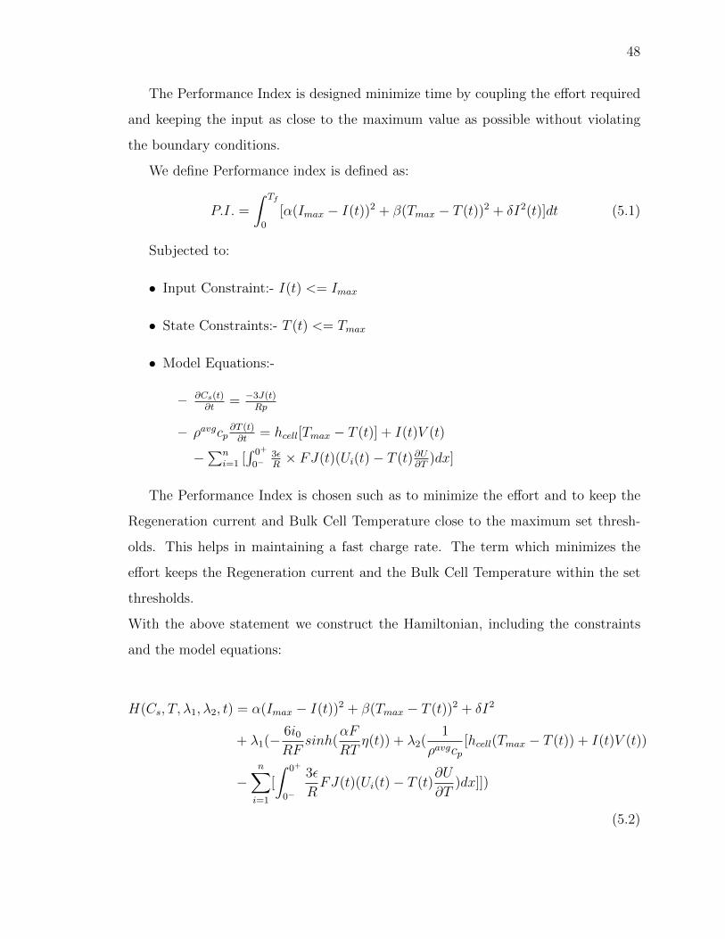
48

The Performance Index is designed minimize time by coupling the effort required

and keeping the input as close to the maximum value as possible without violating

the boundary conditions.

We define Performance index is defined as:

P.I. =

∫ Tf

0

[α(Imax − I(t))2 + β(Tmax − T (t))2 + δI2(t)]dt (5.1)

Subjected to:

• Input Constraint:- I(t) <= Imax

• State Constraints:- T (t) <= Tmax

• Model Equations:-

– ∂Cs(t)∂t

= −3J(t)Rp

– ρavgcp∂T (t)∂t

= hcell[Tmax − T (t)] + I(t)V (t)

−∑n

i=1 [∫ 0+

0−3εR× FJ(t)(Ui(t)− T (t)∂U

∂T)dx]

The Performance Index is chosen such as to minimize the effort and to keep the

Regeneration current and Bulk Cell Temperature close to the maximum set thresh-

olds. This helps in maintaining a fast charge rate. The term which minimizes the

effort keeps the Regeneration current and the Bulk Cell Temperature within the set

thresholds.

With the above statement we construct the Hamiltonian, including the constraints

and the model equations:

H(Cs, T, λ1, λ2, t) = α(Imax − I(t))2 + β(Tmax − T (t))2 + δI2

+ λ1(− 6i0RF

sinh(αF

RTη(t)) + λ2(

1

ρavgcp[hcell(Tmax − T (t)) + I(t)V (t))

−n∑i=1

[

∫ 0+

0−

3ε

RFJ(t)(Ui(t)− T (t)

∂U

∂T)dx]])

(5.2)

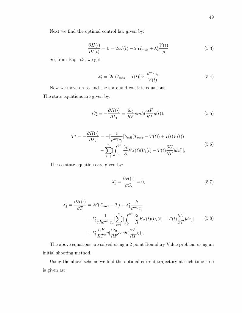
49

Next we find the optimal control law given by:

∂H(·)∂I(t)

= 0 = 2αI(t)− 2αImax + λ∗2V (t)

ρ(5.3)

So, from E.q: 5.3, we get:

λ∗2 = [2α(Imax − I(t)]× ρavgcpV (t)

(5.4)

Now we move on to find the state and co-state equations.

The state equations are given by:

C∗s = −∂H(·)∂λ1

=6i0RF

sinh(αF

RTη(t)), (5.5)

T ∗ = −∂H(·)∂λ2

= −[1

ρavgcp[hcell(Tmax − T (t)) + I(t)V (t))

−n∑i=1

[

∫ 0+

0−

3ε

RFJ(t)(Ui(t)− T (t)

∂U

∂T)dx]]],

(5.6)

The co-state equations are given by:

λ∗1 =∂H(·)∂Cs

= 0, (5.7)

λ∗2 =∂H(·)∂T

= 2β(Tmax − T ) + λ∗2h

ρavgcp

− λ∗21

rhoavgcp[n∑i=1

[

∫ 0+

0−

3ε

RFJ(t)(Ui(t)− T (t)

∂U

∂T)dx]]

+ λ∗1αF

RT 2η[

6i0RF

cosh(αF

RTη)],

(5.8)

The above equations are solved using a 2 point Boundary Value problem using an

initial shooting method.

Using the above scheme we find the optimal current trajectory at each time step

is given as:

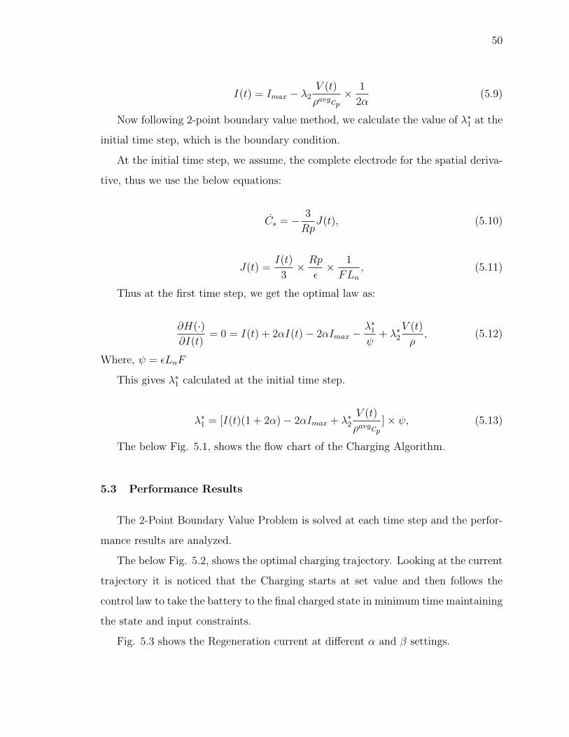
50

I(t) = Imax − λ2V (t)

ρavgcp× 1

2α(5.9)

Now following 2-point boundary value method, we calculate the value of λ∗1 at the

initial time step, which is the boundary condition.

At the initial time step, we assume, the complete electrode for the spatial deriva-

tive, thus we use the below equations:

Cs = − 3

RpJ(t), (5.10)

J(t) =I(t)

3× Rp

ε× 1

FLn, (5.11)

Thus at the first time step, we get the optimal law as:

∂H(·)∂I(t)

= 0 = I(t) + 2αI(t)− 2αImax −λ∗1ψ

+ λ∗2V (t)

ρ, (5.12)

Where, ψ = εLnF

This gives λ∗1 calculated at the initial time step.

λ∗1 = [I(t)(1 + 2α)− 2αImax + λ∗2V (t)

ρavgcp]× ψ, (5.13)

The below Fig. 5.1, shows the flow chart of the Charging Algorithm.

5.3 Performance Results

The 2-Point Boundary Value Problem is solved at each time step and the perfor-

mance results are analyzed.

The below Fig. 5.2, shows the optimal charging trajectory. Looking at the current

trajectory it is noticed that the Charging starts at set value and then follows the

control law to take the battery to the final charged state in minimum time maintaining

the state and input constraints.

Fig. 5.3 shows the Regeneration current at different α and β settings.

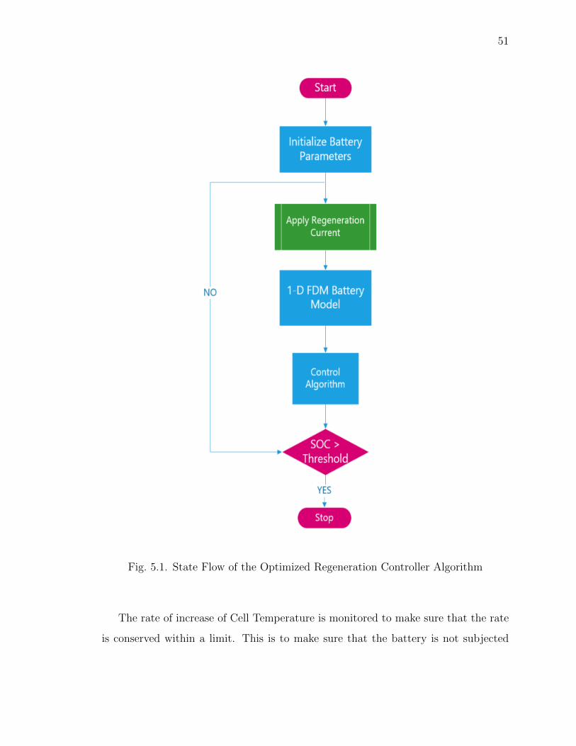
51

Fig. 5.1. State Flow of the Optimized Regeneration Controller Algorithm

The rate of increase of Cell Temperature is monitored to make sure that the rate

is conserved within a limit. This is to make sure that the battery is not subjected

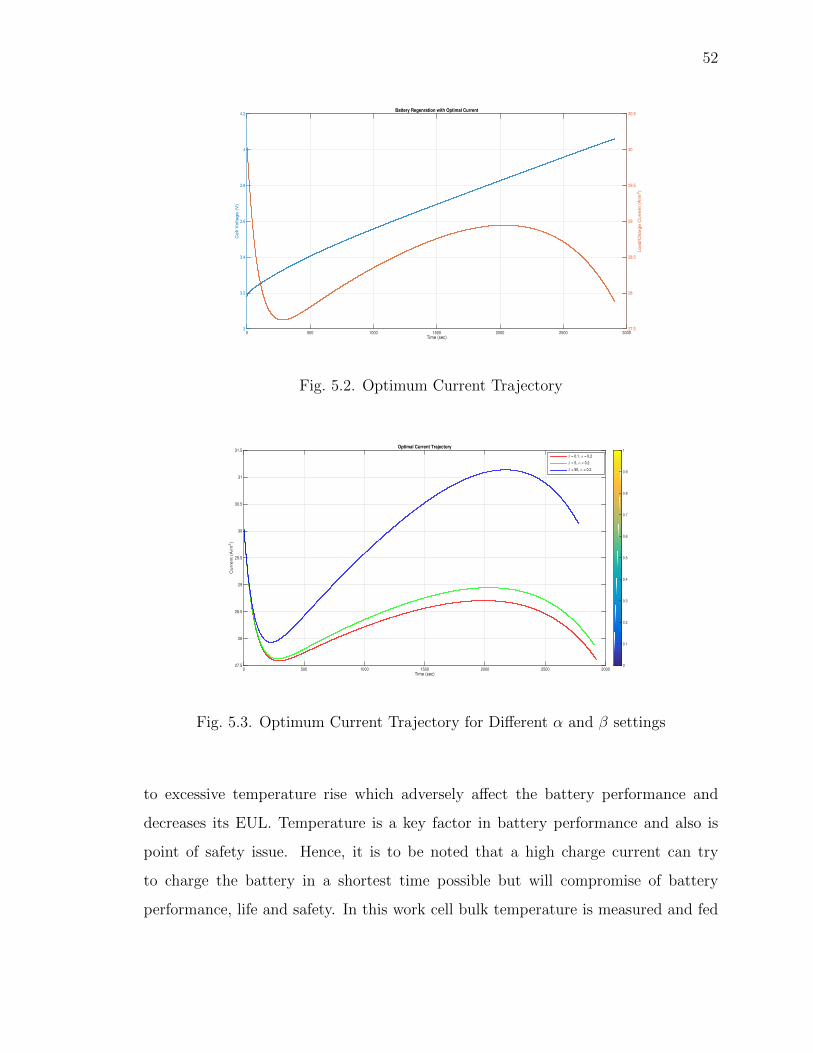
52

Time (sec)0 500 1000 1500 2000 2500 3000

Cell V

oltage (

V)

3

3.2

3.4

3.6

3.8

4

4.2Battery Regenration with Optimal Current

Load/C

harg

e C

urr

ent (A

/m2)

27.5

28

28.5

29

29.5

30

30.5

Fig. 5.2. Optimum Current Trajectory

Time (sec)0 500 1000 1500 2000 2500 3000

Curr

ent (A

/m2)

27.5

28

28.5

29

29.5

30

30.5

31

31.5Optimal Current Trajectory

0

0.1

0.2

0.3

0.4

0.5

0.6

0.7

0.8

0.9

1

β = 0.1, α = 0.2

β = 5, α = 0.2

β = 50, α = 0.2

Fig. 5.3. Optimum Current Trajectory for Different α and β settings

to excessive temperature rise which adversely affect the battery performance and

decreases its EUL. Temperature is a key factor in battery performance and also is

point of safety issue. Hence, it is to be noted that a high charge current can try

to charge the battery in a shortest time possible but will compromise of battery

performance, life and safety. In this work cell bulk temperature is measured and fed

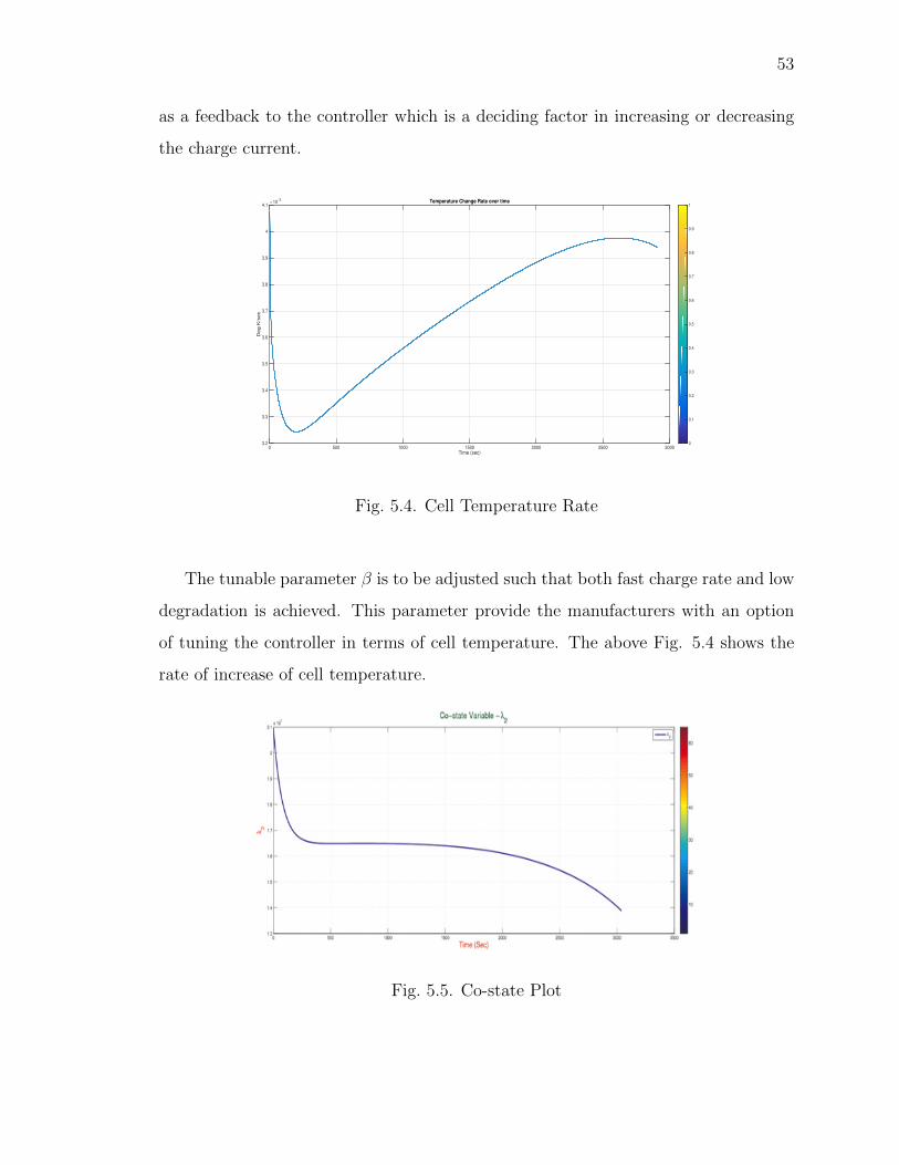
53

as a feedback to the controller which is a deciding factor in increasing or decreasing

the charge current.

Time (sec)0 500 1000 1500 2000 2500 3000

De

g K

/se

c

×10-3

3.2

3.3

3.4

3.5

3.6

3.7

3.8

3.9

4

4.1Temperature Change Rate over time

0

0.1

0.2

0.3

0.4

0.5

0.6

0.7

0.8

0.9

1

Fig. 5.4. Cell Temperature Rate

The tunable parameter β is to be adjusted such that both fast charge rate and low

degradation is achieved. This parameter provide the manufacturers with an option

of tuning the controller in terms of cell temperature. The above Fig. 5.4 shows the

rate of increase of cell temperature.

Fig. 5.5. Co-state Plot

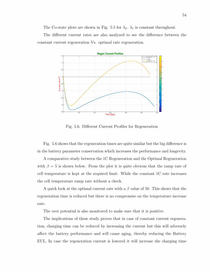
54

The Co-state plots are shown in Fig. 5.5 for λ2. λ1 is constant throughout.

The different current rates are also analyzed to see the difference between the

constant current regeneration Vs. optimal rate regeneration.

Time (Sec)0 500 1000 1500 2000 2500 3000

Cu

rre

nt

(A/m

2)

27.5

28

28.5

29

29.5

30

30.5

31

31.5

Regen Current Profiles

0

0.1

0.2

0.3

0.4

0.5

0.6

0.7

0.8

0.9

1

Opt Regen @ β = 5

1C Regen

Opt Regen @ β = 50

Fig. 5.6. Different Current Profiles for Regeneration

Fig. 5.6 shows that the regeneration times are quite similar but the big difference is

in the battery parameter conservation which increases the performance and longevity.

A comparative study between the 1C Regeneration and the Optimal Regeneration

with β = 5 is shown below. From the plot it is quite obvious that the ramp rate of

cell temperature is kept at the required limit. While the constant 1C rate increases

the cell temperature ramp rate without a check.

A quick look at the optimal current rate with a β value of 50. This shows that the

regeneration time is reduced but there is no compromise on the temperature increase

rate.

The over potential is also monitored to make sure that it is positive.

The implications of these study proves that in case of constant current regenera-

tion, charging time can be reduced by increasing the current but this will adversely

affect the battery performance and will cause aging, thereby reducing the Battery

EUL. In case the regeneration current is lowered it will increase the charging time

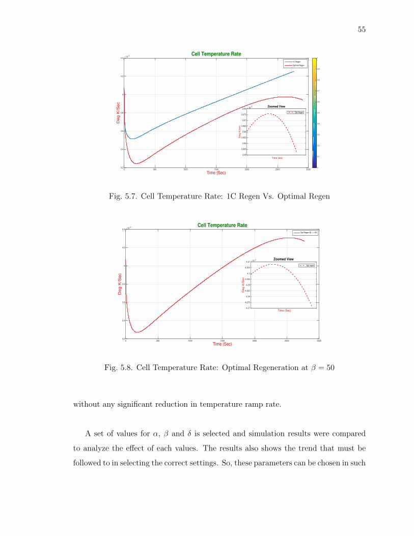
55

Time (Sec)0 500 1000 1500 2000 2500 3000

De

g K

/Se

c

×10-3

3.2

3.4

3.6

3.8

4

4.2

4.4

Cell Temperature Rate

0

0.1

0.2

0.3

0.4

0.5

0.6

0.7

0.8

0.9

1

1C Regen

Optimal Regen

Time (sec)

Deg K

/sec

×10-3

3.94

3.945

3.95

3.955

3.96

3.965

3.97

3.975

3.98Zoomed View

Opt Regen

Fig. 5.7. Cell Temperature Rate: 1C Regen Vs. Optimal Regen

Time (Sec)0 500 1000 1500 2000 2500 3000

De

g K

/Se

c

×10-3

3.2

3.4

3.6

3.8

4

4.2

4.4

Cell Temperature RateOpt Regen @ β = 50

Time (Sec)

Deg K

/Sec

×10-3

4.27

4.275

4.28

4.285

4.29

4.295

4.3

4.305

4.31Zoomed View

Opt regen

Fig. 5.8. Cell Temperature Rate: Optimal Regeneration at β = 50

without any significant reduction in temperature ramp rate.

A set of values for α, β and δ is selected and simulation results were compared

to analyze the effect of each values. The results also shows the trend that must be

followed to in selecting the correct settings. So, these parameters can be chosen in such

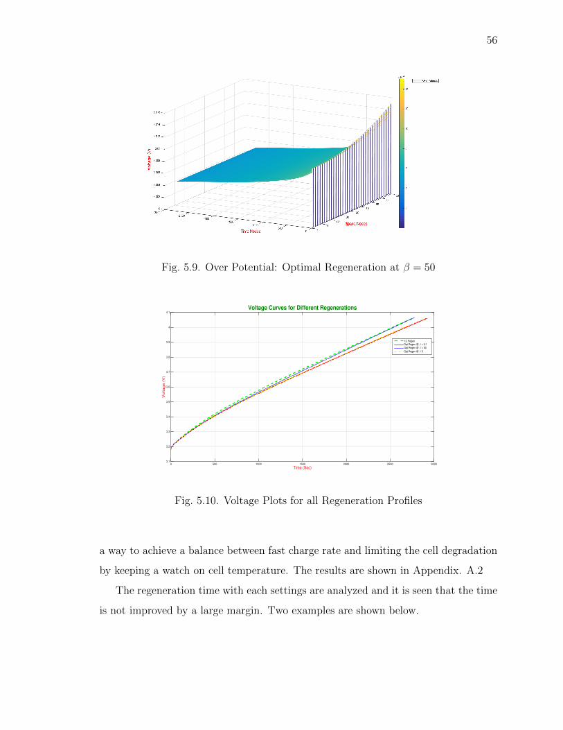
56

Fig. 5.9. Over Potential: Optimal Regeneration at β = 50

Time (Sec)0 500 1000 1500 2000 2500 3000

Voltage (

V)

3.1

3.2

3.3

3.4

3.5

3.6

3.7

3.8

3.9

4

4.1Voltage Curves for Different Regenerations

1C RegenOpt Regen @ β = 0.1

Opt Regen @ β = 50

Opt Regen @ β 5

Fig. 5.10. Voltage Plots for all Regeneration Profiles

a way to achieve a balance between fast charge rate and limiting the cell degradation

by keeping a watch on cell temperature. The results are shown in Appendix. A.2

The regeneration time with each settings are analyzed and it is seen that the time

is not improved by a large margin. Two examples are shown below.

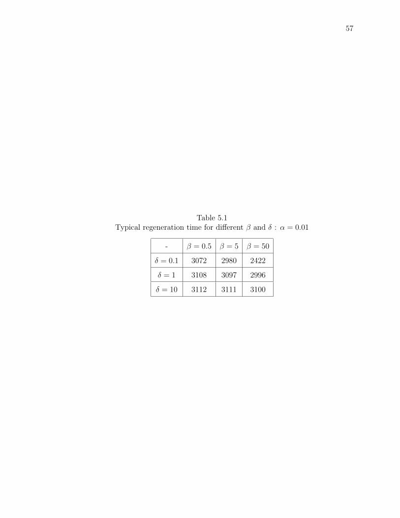
57

Table 5.1Typical regeneration time for different β and δ : α = 0.01

- β = 0.5 β = 5 β = 50

δ = 0.1 3072 2980 2422

δ = 1 3108 3097 2996

δ = 10 3112 3111 3100

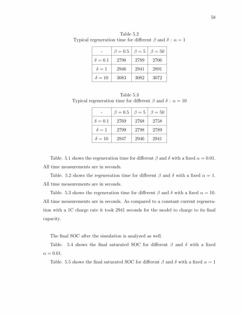
58

Table 5.2Typical regeneration time for different β and δ : α = 1

- β = 0.5 β = 5 β = 50

δ = 0.1 2798 2789 2706

δ = 1 2946 2941 2891

δ = 10 3083 3082 3072

Table 5.3Typical regeneration time for different β and δ : α = 10

- β = 0.5 β = 5 β = 50

δ = 0.1 2769 2768 2758

δ = 1 2799 2798 2789

δ = 10 2947 2946 2941

Table. 5.1 shows the regeneration time for different β and δ with a fixed α = 0.01.

All time measurements are in seconds.

Table. 5.2 shows the regeneration time for different β and δ with a fixed α = 1.

All time measurements are in seconds.

Table. 5.3 shows the regeneration time for different β and δ with a fixed α = 10.

All time measurements are in seconds. As compared to a constant current regenera-

tion with a 1C charge rate it took 2941 seconds for the model to charge to its final

capacity.

The final SOC after the simulation is analyzed as well.

Table. 5.4 shows the final saturated SOC for different β and δ with a fixed

α = 0.01.

Table. 5.5 shows the final saturated SOC for different β and δ with a fixed α = 1

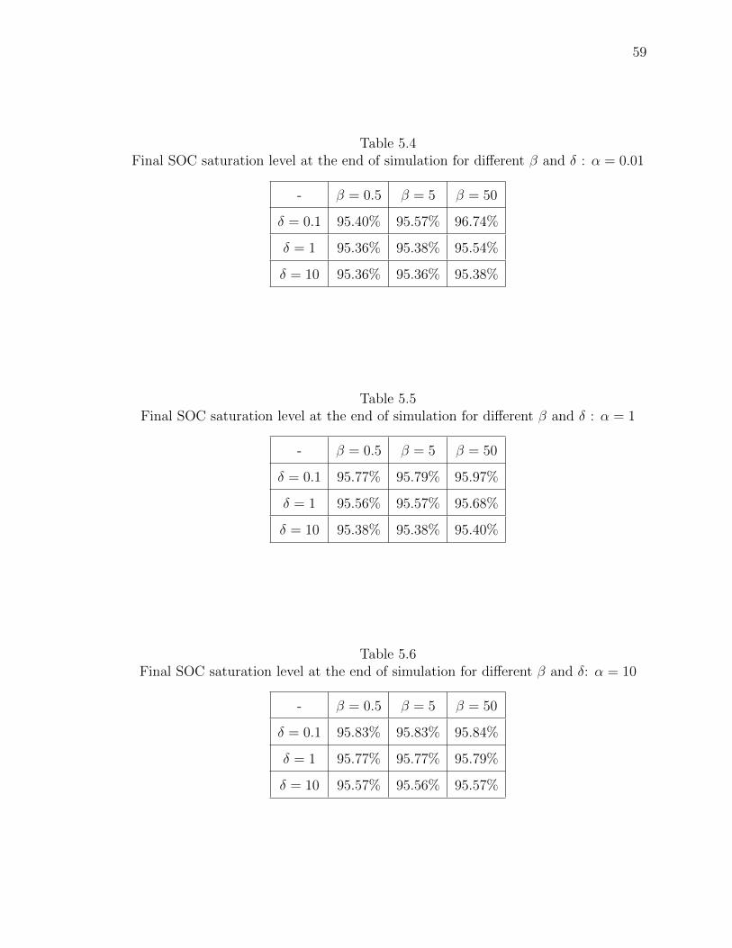
59

Table 5.4Final SOC saturation level at the end of simulation for different β and δ : α = 0.01

- β = 0.5 β = 5 β = 50

δ = 0.1 95.40% 95.57% 96.74%

δ = 1 95.36% 95.38% 95.54%

δ = 10 95.36% 95.36% 95.38%

Table 5.5Final SOC saturation level at the end of simulation for different β and δ : α = 1

- β = 0.5 β = 5 β = 50

δ = 0.1 95.77% 95.79% 95.97%

δ = 1 95.56% 95.57% 95.68%

δ = 10 95.38% 95.38% 95.40%

Table 5.6Final SOC saturation level at the end of simulation for different β and δ: α = 10

- β = 0.5 β = 5 β = 50

δ = 0.1 95.83% 95.83% 95.84%

δ = 1 95.77% 95.77% 95.79%

δ = 10 95.57% 95.56% 95.57%

60

Table. 5.6 shows the final saturated SOC for different β and δ with a fixed

α = 10.

Thus, we have seen that the present results are quite promising. The two tuning

parameters α and β can be used to their fullest potential to achieve better results for

all variety of battery state parameters. It is also noted that the regeneration current

is not following a conventional steady state trends but rather it follows a continuous

and smooth curve. While this increases a bit of hard wire change but with the current

PWM switching frequency oscillators this is not impossible. Also, with a constant

current - constant voltage there is a chance of pushing the batteries to its limits with

out any feedback monitoring system of the battery internal states. In this scheme the

battery states are continuously monitored in terms of temperature and its co-states.

This gives a better internal state management system of the battery.

The cell model assumes an ideal electro-chemical cell and ignores any cell degra-

dation mechanisms that may result from any extreme cell designs. These mechanisms

are important when considering the overall life cycle performance. A cell design that

has maximum initial energy density or performance only to suffer catastrophic ca-

pacity loss or power fade within a small number of cycles would be a poor design.

Additional constraints that set lower bounds on the end-of-life energy density or mod-

ifications to the objective function that accounts for cumulative useful energy over the

entire lifetime should be included. Another important aspect is the volume fraction

change. Volume fraction change in the graphite anode and manganese spinel cathode

is small and is neglected in the cell model, however it is not the case for some of

the other materials, such as silicon in anodes. Volume change up to factors of 3 4

can be expected during intercalation. The large volume increase means that the ion

transport equation in the solid phase cannot be simplified to the diffusion equation.

Volume change in electrode causes [54]:

• Change in porosity

• Cell impedance

61

• Loss of power

• Contact loss of active materials

• Capacity fade

Accounting for the effects of volume expansion in the cell model requires cou-

pling of a physics-based degradation model to determine how design variables, such

as particle size and volume fraction, contribute to contact loss. Factors such as par-

ticle packing density and size influence the effect of volume change [55] needs to be

considered as well.

One of the primary causes of lithium loss in the cell is the decomposition of

electrolyte at the negative electrode/electrolyte interface to form a passive SEI layer

during the initial cycles [54]. This is due to the anode operating at voltages that are

outside the electrochemical stability window of electrolyte components. SEI formation

is an irreversible process that consumes reusable lithium. However the SEI layer is

also beneficial in preventing further decomposition of solvent and at the same time

allows lithium ions to pass through. To accurately model the formation, growth

and subsequent stabilization of SEI layer, physics-based interaction between electrode

active material and electrolyte and influence of SEI thickness on electrolyte diffusivity

should be included in the cell model [56].

Volume change in the cell and SEI formation affects the intercalation induced

stress on the solid particles. The amount of stress depends on the shape and size of

particles, and it is interrelated through the local surface flux, and ion concentration

gradient [57]. Multi-scale modeling has shown that lithium intercalation for large

particles is diffusion limited and that the resulting diffusion-stress coupling causes

mismatching strains and stresses [58]. High stress is also experienced in nano-scale

particles due to surface stress effect [59].

62

6. CONCLUSIONS AND RECOMMENDATIONS

6.1 Concluding Summary

The 1-D Cell model is validated against published papers to substantiate its per-

formance against all operating regions.The different C-Rate charge/discharge cycles

shows promising results.

The optimal charging algorithm developed in this literature is based on the fol-

lowing battery state parameters:

• State of charge - SOC(t)

• Solid Phase concentration - Cs(t)

• Molar Flux - J(t)

• Cell Temperature - T (t)

• Over potential - η(t)

The control law behaved well with both, input and state constraints. Though

battery internal degradation is not dynamically modeled, but it is observed that ne-

glecting these factors did not affect the simulation result much.

A set of 3 point values were used for each α, β and δ and the simulation results

are presented in Appendix B.

Based on the current and voltage profile along with the cell temperature rate 2 sets of

optimized and tuned values are proposed. Table. 6.1 shows the tuned set of proposed

values.

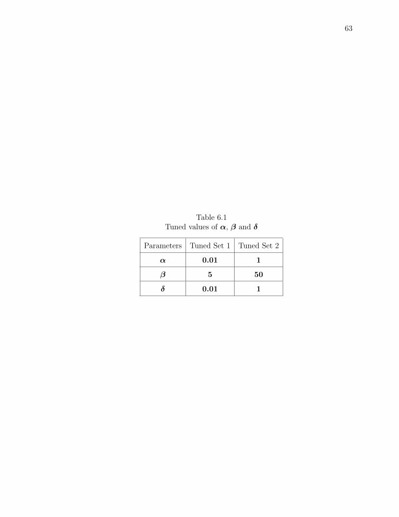
63

Table 6.1Tuned values of α, β and δ

Parameters Tuned Set 1 Tuned Set 2

α 0.01 1

β 5 50

δ 0.01 1

64

6.2 Major contribution on the Thesis

This thesis work is focused to improve two major aspects of 1-D Lithium Battery

BMS system. Though many small factors are touched upon and discussed in this

work like cell volume change, stresses in the cell and resistance formation and their

relation to bulk cell temperature, the primary two major improvements discussed and

supported in this work are:

• Robust numerical solution framework for reformulated physics based 1-D model.

• A dynamic closed loop efficient optimization technique for battery regeneration.

The numerical framework designed in this work is a multi purpose model which is

capable of running all battery cycles with high fidelity. Simulation of the numerical

method showed that the model replicates the actual cell characteristics and behavior

for almost any cycle. Cell bulk temperature which is one of the key contributor to

many other battery states and its performance is also modeled very accurately in

this model. The numerical method of solving the battery equations can be used

to solve battery dynamics required in any application where a physics based model

is desired.The next big improvement is obviously the optimization method and the

performance achieved. Contrary to the conventional CC-CV method this is more

dynamical and more close to following the battery internal chemistry. In traditional

CC-CV process apart from the basic safety feature which tends to switch the charging

current from one level to the other so as to keep a check on the temperature there

is no other close loop action or monitoring of the internal battery kinetics. With

this proposed optimization scheme there is a huge leap towards including the cell

temperature and other battery internal states into the calculation of charging current.

This brings in a balance between both performance and battery degradation and

performs an optimized charging action. This is a big improvement when battery life

and aging is considered.

65

6.3 Recommendations for Future Work

As stated earlier, future work is to include physical measurable state parameters

from the battery and manipulate the optimal law to include only those parameters.

The next big step shall be to include the control algorithm into hardware in loop

and quantify the performance of the algorithm. Experiments with actual battery cell

along with battery pack is required to come up with optimized tuned values for α,

β and δ parameters. This simulations with actual cell will also indicate the level of

improvements based on aging and degradation of the battery. Future work shall focus

deeply on the effects of battery state parameters on resistive film formation across the

electrodes. It is also require to analyze the effects of these resistive films on battery

performance, especially when the battery reaches it EUL. A more advanced study is

recommended to analyze the effects of altering the battery internal states by external

perturbation so as to increase the battery performance. This is a very abstract level

notion which could be pondered upon to get beneficial results.

LIST OF REFERENCES

66

LIST OF REFERENCES

[1] N. Xue, Design and Optimization of Lithium-Ion Batteries for Electric-VehicleApplications. PhD thesis, University of Michigan, 2014.

[2] E. I. Administration and U. D. of Energy, “Eia. annual energy review,” 2011.

[3] U. S. E. P. Agency, “Eia. inventory of u.s. greenhouse gas emissions and sinks:,”2013.

[4] T. K. S. of Automotive Engineers (KSAE), “Elec-tric vehicles in asia pacific: What is electric vechicle?.”http://www.evaap.org/electric/electric.html?sgubun=1 (Last Accessed:21 January 2015).

[5] B. University, “Charging lithium ion batteries.” Last Accessed: 21 January 2015.

[6] D. X. Chen, “Illustration of the charge/discharge processes in rechargeablelithium ion.” http://cas.umkc.edu/chemistry/chen.asp (Last Accessed: 21January 2015).

[7] M. Doyle, T. F. Fuller, and J. Newman, “Modeling of galvanostatic charge anddischarge of the lithium/polymer/insertion cell,” Journal of The ElectrochemicalSociety, vol. 140, no. 6, pp. 1526–1533, 1993.

[8] R. Klein, N. A. Chaturvedi, J. Christensen, J. Ahmed, R. Findeisen, and A. Ko-jic, “Optimal charging strategies in lithium-ion battery,” American Control Con-ference, 2011.

[9] N. Chaturvedi, R. Klein, J. Christensen, J. Ahmed, and A. Kojic, “Algorithmsfor advanced battery management systems: Modeling, estimation, and controlchallenges for lithium-ion batteries,” IEEE Control Systems Magazine, vol. 30,no. 3, 2010.

[10] V. Ramadesigan, P. W. C. Northrop, S. De, S. Santhanagopalan, R. D. Braatz,and V. R. Subramanian, “Modeling and simulation of lithium-ion batteriesfrom a systems engineering perspective,” Journal of The Electrochemical Society,vol. 159, no. 3, pp. 31–45, 2012.

[11] D. Zhang, B. N. Popov, and R. E. White Journal of The Electrochemical Society,vol. 147, p. 831, 2000.

[12] S. Santhanagopalan, Q. Z. Guo, P. Ramadass, and R. E. White Journal of TheElectrochemical Society, vol. 156, p. 620, 2006.

[13] M. Doyle and J. Newman, “Effects of diffusive charge transfer and salt con-centration gradient in electrolyte on li-ion battery energy and power densities,”Journal of The Electrochemical Society, vol. 40, p. 2191, 1995.

67

[14] J. Newman Journal of The Electrochemical Society, vol. 142, p. 97, 1995.

[15] P. Arora, M. Doyle, A. S. Gozdz, R. E. White, and J. Newman Journal of TheElectrochemical Society, vol. 88, p. 219, 2000.

[16] G. G. Botte, V. R. Subramanian, and R. E. White Journal of The ElectrochemicalSociety, vol. 45, p. 2595, 2000.

[17] M. Doyle, J. Newman, A. S. Gozdz, C. N. Schmutz, and J. M. Tarascon Journalof The Electrochemical Society, vol. 143, p. 1890, 1996.

[18] T. F. Fuller, M. Doyle, and J. Newman Journal of The Electrochemical Society,vol. 141, p. 982, 1994.

[19] T. F. Fuller, M. Doyle, and J. Newman Journal of The Electrochemical Society,vol. 141, p. 1, 1994.

[20] P. M. Gomadam, J. W. Weidner, R. A. Dougal, and R. E. White Journal of TheElectrochemical Society, vol. 110, p. 267, 2002.

[21] J. Newman and W. Tiedemann AIChE, vol. 21, p. 25, 1975.

[22] G. Ning, R. E. White, and B. N. Popov Electrochim Acta, vol. 51, p. 2012, 2006.

[23] P. Ramadass, B. Haran, P. M. Gomadam, R. White, and B. N. Popov, “Devel-opment of first principles capacity fade model for li-ion cells,” Journal of TheElectrochemical Society, vol. 151, p. A196, 2004.

[24] P. Ramadass, B. Haran, R. White, and B. N. Popov J Power Sources, vol. 123,p. 230, 2003.

[25] K. E. Thomas and J. Newman Journal of The Electrochemical Society, vol. 150,p. A176, 2003.

[26] S. A. Hallaj, H. Maleki, J. S. Hong, and J. R. Selman J Power Sources, vol. 83,p. 1, 1999.

[27] T. I. Evans and R. E. White, “A thermal analysis of a spirally wound batteryusing a simple mathematical model,” Journal of The Electrochemical Society,vol. 136, p. 2145, 1989.

[28] D. Bernardi, E. Pawlikowski, and J. Newman Journal of The ElectrochemicalSociety, vol. 132, p. 5, 1985.

[29] Y. Chen and J. W. Evans Journal of The Electrochemical Society, vol. 140,p. 1833, 1993.

[30] Y. F. Chen and J. W. Evans Journal of The Electrochemical Society, vol. 141,p. 2947, 1994.

[31] C. R. Pals and J. Newman Journal of The Electrochemical Society, vol. 142,p. 3274, 1995.

[32] C. R. Pals and J. Newman, “The effect of battery design parameters on heatgeneration and utilization in a li-ion cell,” Journal of The Electrochemical Society,vol. 142, p. 3282, 1995.

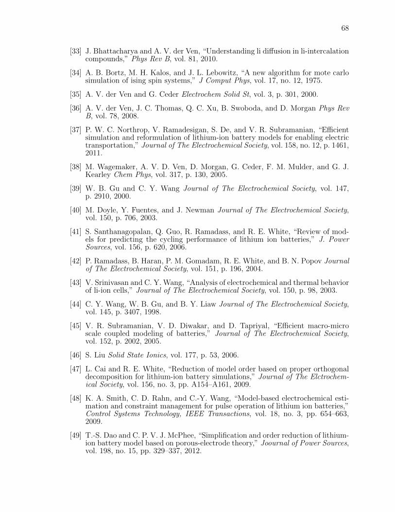
68

[33] J. Bhattacharya and A. V. der Ven, “Understanding li diffusion in li-intercalationcompounds,” Phys Rev B, vol. 81, 2010.

[34] A. B. Bortz, M. H. Kalos, and J. L. Lebowitz, “A new algorithm for mote carlosimulation of ising spin systems,” J Comput Phys, vol. 17, no. 12, 1975.

[35] A. V. der Ven and G. Ceder Electrochem Solid St, vol. 3, p. 301, 2000.

[36] A. V. der Ven, J. C. Thomas, Q. C. Xu, B. Swoboda, and D. Morgan Phys RevB, vol. 78, 2008.

[37] P. W. C. Northrop, V. Ramadesigan, S. De, and V. R. Subramanian, “Efficientsimulation and reformulation of lithium-ion battery models for enabling electrictransportation,” Journal of The Electrochemical Society, vol. 158, no. 12, p. 1461,2011.

[38] M. Wagemaker, A. V. D. Ven, D. Morgan, G. Ceder, F. M. Mulder, and G. J.Kearley Chem Phys, vol. 317, p. 130, 2005.

[39] W. B. Gu and C. Y. Wang Journal of The Electrochemical Society, vol. 147,p. 2910, 2000.

[40] M. Doyle, Y. Fuentes, and J. Newman Journal of The Electrochemical Society,vol. 150, p. 706, 2003.

[41] S. Santhanagopalan, Q. Guo, R. Ramadass, and R. E. White, “Review of mod-els for predicting the cycling performance of lithium ion batteries,” J. PowerSources, vol. 156, p. 620, 2006.

[42] P. Ramadass, B. Haran, P. M. Gomadam, R. E. White, and B. N. Popov Journalof The Electrochemical Society, vol. 151, p. 196, 2004.

[43] V. Srinivasan and C. Y. Wang, “Analysis of electrochemical and thermal behaviorof li-ion cells,” Journal of The Electrochemical Society, vol. 150, p. 98, 2003.

[44] C. Y. Wang, W. B. Gu, and B. Y. Liaw Journal of The Electrochemical Society,vol. 145, p. 3407, 1998.

[45] V. R. Subramanian, V. D. Diwakar, and D. Tapriyal, “Efficient macro-microscale coupled modeling of batteries,” Journal of The Electrochemical Society,vol. 152, p. 2002, 2005.

[46] S. Liu Solid State Ionics, vol. 177, p. 53, 2006.

[47] L. Cai and R. E. White, “Reduction of model order based on proper orthogonaldecomposition for lithium-ion battery simulations,” Journal of The Elctrochem-ical Society, vol. 156, no. 3, pp. A154–A161, 2009.

[48] K. A. Smith, C. D. Rahn, and C.-Y. Wang, “Model-based electrochemical esti-mation and constraint management for pulse operation of lithium ion batteries,”Control Systems Technology, IEEE Transactions, vol. 18, no. 3, pp. 654–663,2009.

[49] T.-S. Dao and C. P. V. J. McPhee, “Simplification and order reduction of lithium-ion battery model based on porous-electrode theory,” Joournal of Power Sources,vol. 198, no. 15, pp. 329–337, 2012.

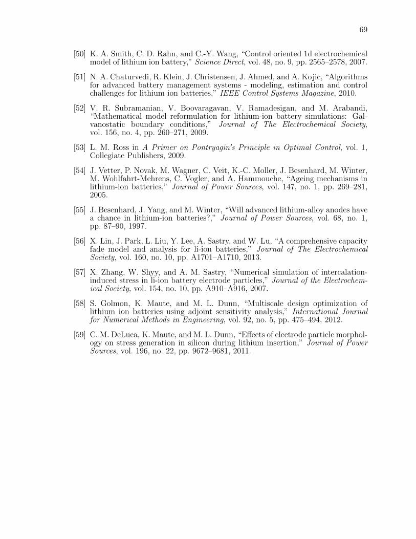
69

[50] K. A. Smith, C. D. Rahn, and C.-Y. Wang, “Control oriented 1d electrochemicalmodel of lithium ion battery,” Science Direct, vol. 48, no. 9, pp. 2565–2578, 2007.

[51] N. A. Chaturvedi, R. Klein, J. Christensen, J. Ahmed, and A. Kojic, “Algorithmsfor advanced battery management systems - modeling, estimation and controlchallenges for lithium ion batteries,” IEEE Control Systems Magazine, 2010.

[52] V. R. Subramanian, V. Boovaragavan, V. Ramadesigan, and M. Arabandi,“Mathematical model reformulation for lithium-ion battery simulations: Gal-vanostatic boundary conditions,” Journal of The Electrochemical Society,vol. 156, no. 4, pp. 260–271, 2009.

[53] L. M. Ross in A Primer on Pontryagin’s Principle in Optimal Control, vol. 1,Collegiate Publishers, 2009.

[54] J. Vetter, P. Novak, M. Wagner, C. Veit, K.-C. Moller, J. Besenhard, M. Winter,M. Wohlfahrt-Mehrens, C. Vogler, and A. Hammouche, “Ageing mechanisms inlithium-ion batteries,” Journal of Power Sources, vol. 147, no. 1, pp. 269–281,2005.

[55] J. Besenhard, J. Yang, and M. Winter, “Will advanced lithium-alloy anodes havea chance in lithium-ion batteries?,” Journal of Power Sources, vol. 68, no. 1,pp. 87–90, 1997.

[56] X. Lin, J. Park, L. Liu, Y. Lee, A. Sastry, and W. Lu, “A comprehensive capacityfade model and analysis for li-ion batteries,” Journal of The ElectrochemicalSociety, vol. 160, no. 10, pp. A1701–A1710, 2013.

[57] X. Zhang, W. Shyy, and A. M. Sastry, “Numerical simulation of intercalation-induced stress in li-ion battery electrode particles,” Journal of the Electrochem-ical Society, vol. 154, no. 10, pp. A910–A916, 2007.

[58] S. Golmon, K. Maute, and M. L. Dunn, “Multiscale design optimization oflithium ion batteries using adjoint sensitivity analysis,” International Journalfor Numerical Methods in Engineering, vol. 92, no. 5, pp. 475–494, 2012.

[59] C. M. DeLuca, K. Maute, and M. L. Dunn, “Effects of electrode particle morphol-ogy on stress generation in silicon during lithium insertion,” Journal of PowerSources, vol. 196, no. 22, pp. 9672–9681, 2011.

APPENDICES

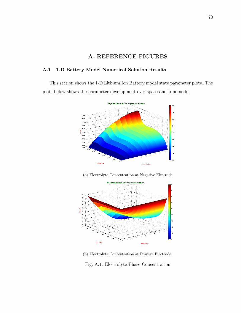
70

A. REFERENCE FIGURES

A.1 1-D Battery Model Numerical Solution Results

This section shows the 1-D Lithium Ion Battery model state parameter plots. The

plots below shows the parameter development over space and time node.

(a) Electrolyte Concentration at Negative Electrode

(b) Electrolyte Concentration at Positive Electrode

Fig. A.1. Electrolyte Phase Concentration

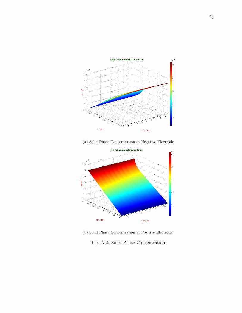
71

(a) Solid Phase Concentration at Negative Electrode

(b) Solid Phase Concentration at Positive Electrode

Fig. A.2. Solid Phase Concentration

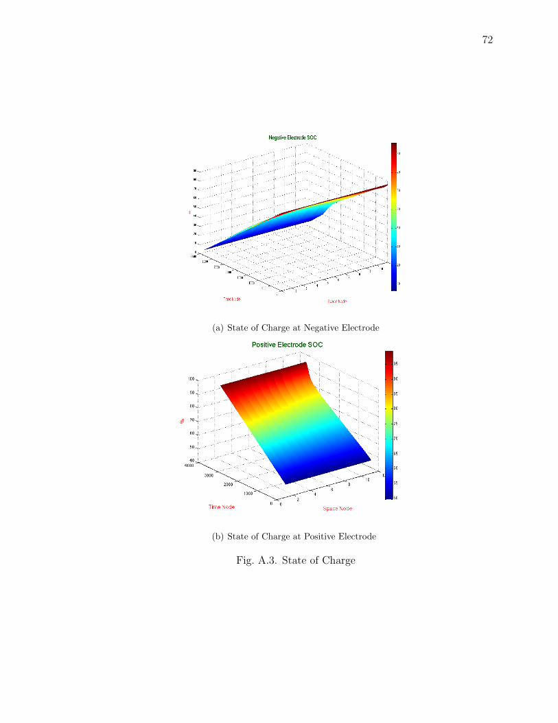
72

(a) State of Charge at Negative Electrode

(b) State of Charge at Positive Electrode

Fig. A.3. State of Charge

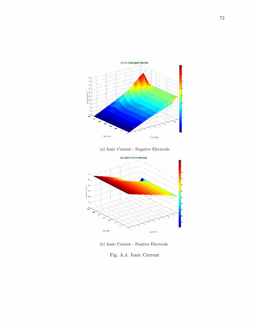
73

(a) Ionic Current - Negative Electrode

(b) Ionic Current - Positive Electrode

Fig. A.4. Ionic Current

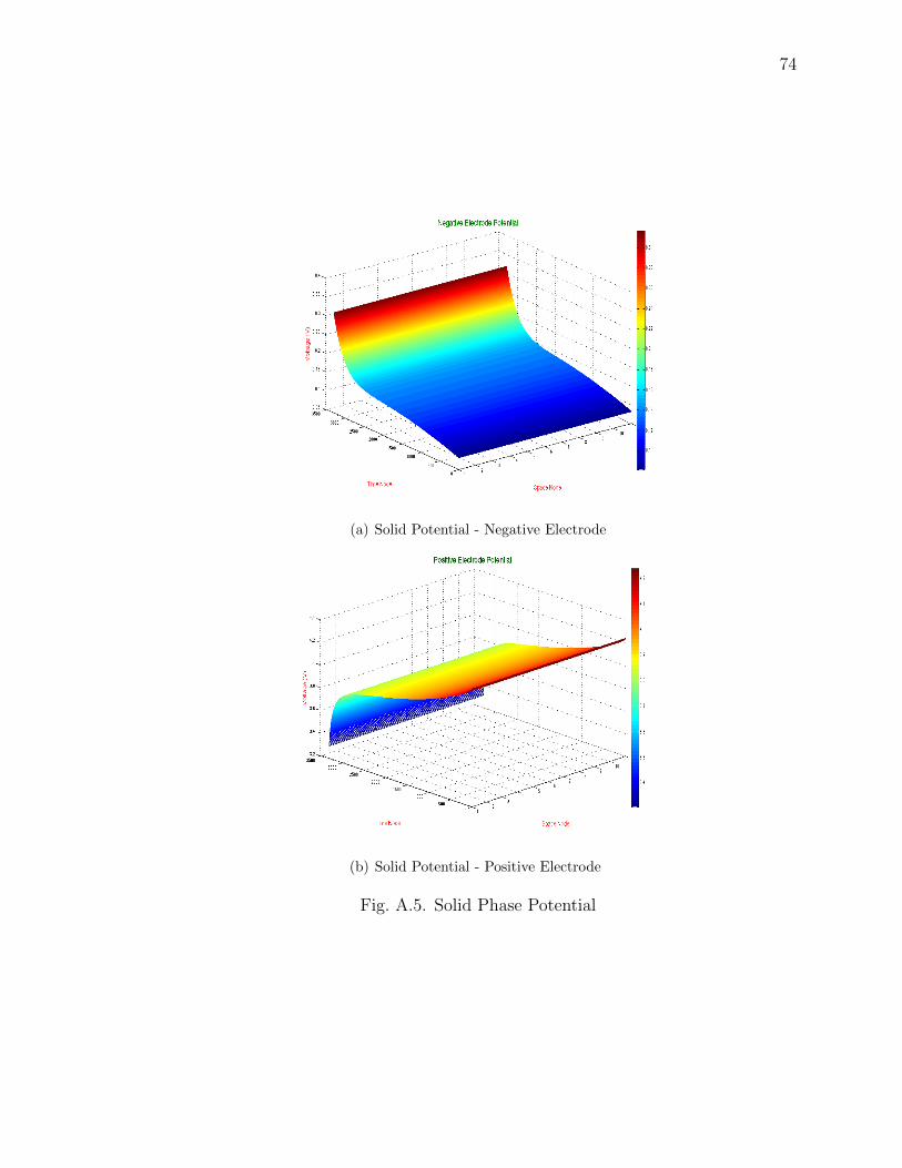
74

(a) Solid Potential - Negative Electrode

(b) Solid Potential - Positive Electrode

Fig. A.5. Solid Phase Potential

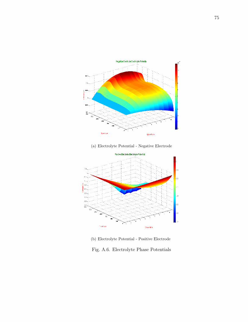
75

(a) Electrolyte Potential - Negative Electrode

(b) Electrolyte Potential - Positive Electrode

Fig. A.6. Electrolyte Phase Potentials

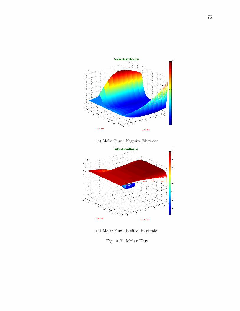
76

(a) Molar Flux - Negative Electrode

(b) Molar Flux - Positive Electrode

Fig. A.7. Molar Flux

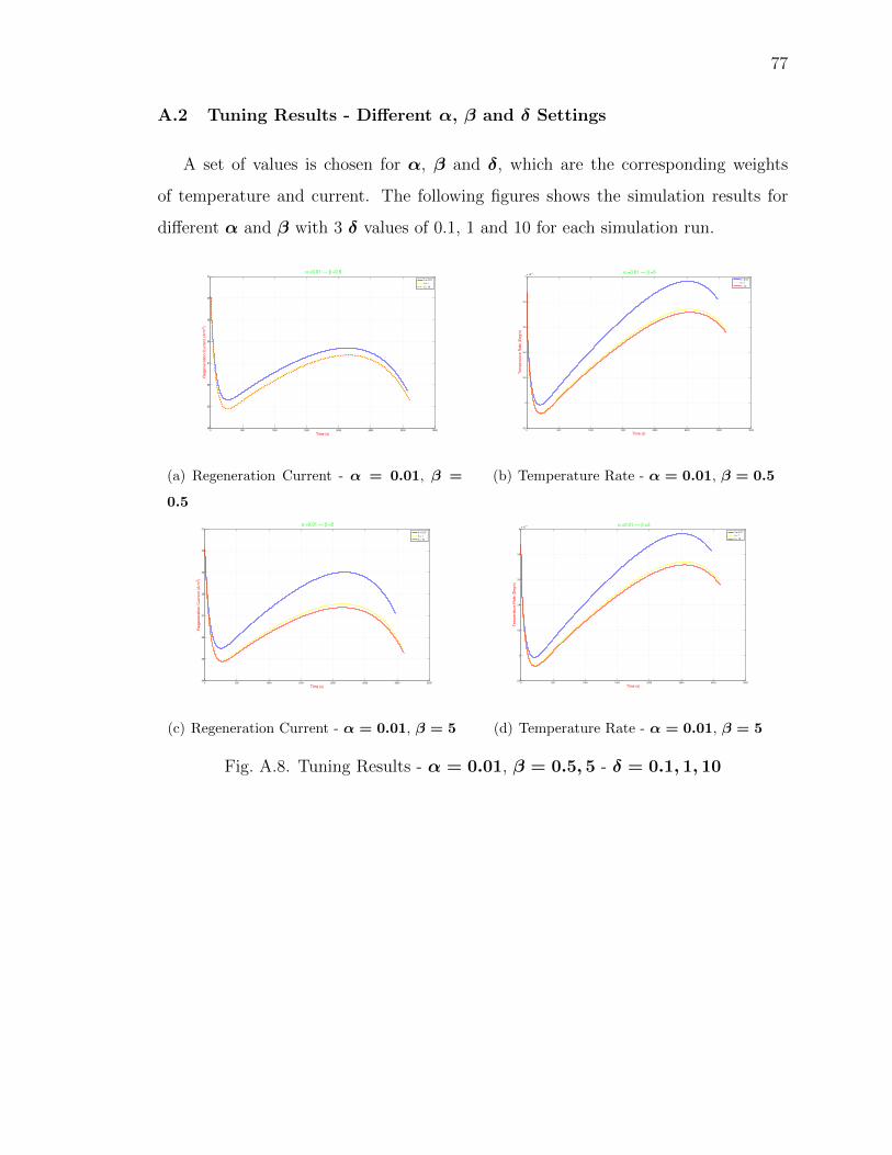
77

A.2 Tuning Results - Different α, β and δ Settings

A set of values is chosen for α, β and δ, which are the corresponding weights

of temperature and current. The following figures shows the simulation results for

different α and β with 3 δ values of 0.1, 1 and 10 for each simulation run.

0 500 1000 1500 2000 2500 3000 350024

25

26

27

28

29

30

31

Time (s)

Re

ge

ne

ratio

n C

urr

en

t (A

/m2)

α =0.01 −− β =0.5

δ = 0.01

δ = 1

δ = 10

(a) Regeneration Current - α = 0.01, β =

0.5

0 500 1000 1500 2000 2500 3000 35002.8

3

3.2

3.4

3.6

3.8

4x 10

−3

Time (s)

Tem

pera

ture

Rate

(D

eg/s

)

α =0.01 −− β =5

δ = 0.01

δ = 1

δ = 10

(b) Temperature Rate - α = 0.01, β = 0.5

0 500 1000 1500 2000 2500 3000 350024

25

26

27

28

29

30

31

Time (s)

Re

ge

ne

ratio

n C

urr

en

t (A

/m2)

α =0.01 −− β =5

δ = 0.01

δ = 1

δ = 10

(c) Regeneration Current - α = 0.01, β = 5

0 500 1000 1500 2000 2500 3000 35002.8

3

3.2

3.4

3.6

3.8

4x 10

−3

Time (s)

Tem

pera

ture

Rate

(D

eg/s

)

α =0.01 −− β =5

δ = 0.01

δ = 1

δ = 10

(d) Temperature Rate - α = 0.01, β = 5

Fig. A.8. Tuning Results - α = 0.01, β = 0.5, 5 - δ = 0.1, 1, 10

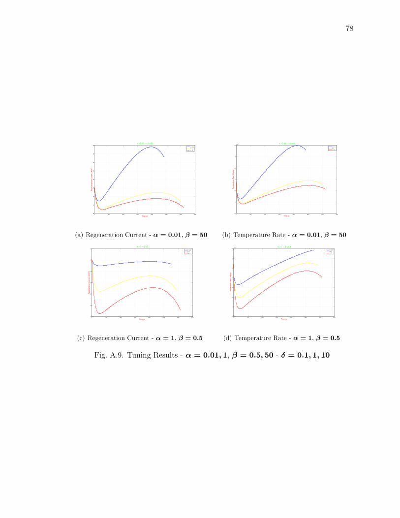
78

0 500 1000 1500 2000 2500 3000 350024

26

28

30

32

34

36

38

40

Time (s)

Re

ge

ne

ratio

n C

urr

en

t (A

/m2)

α =0.01 −− β =50

δ = 0.01

δ = 1

δ = 10

(a) Regeneration Current - α = 0.01, β = 50

0 500 1000 1500 2000 2500 3000 35002.5

3

3.5

4

4.5

5

5.5x 10

−3

Time (s)

Tem

pera

ture

Rate

(D

eg/s

)

α =0.01 −− β =50

δ = 0.01

δ = 1

δ = 10

(b) Temperature Rate - α = 0.01, β = 50

0 500 1000 1500 2000 2500 3000 350025

26

27

28

29

30

31

Time (s)

Re

ge

ne

ratio

n C

urr

en

t (A

/m2)

α =1 −− β =5

δ = 0.01

δ = 1

δ = 10

(c) Regeneration Current - α = 1, β = 0.5

0 500 1000 1500 2000 2500 3000 35002.8

3

3.2

3.4

3.6

3.8

4

4.2x 10

−3

Time (s)

Tem

pera

ture

Rate

(D

eg/s

)

α =1 −− β =0.5

δ = 0.01

δ = 1

δ = 10

(d) Temperature Rate - α = 1, β = 0.5

Fig. A.9. Tuning Results - α = 0.01, 1, β = 0.5, 50 - δ = 0.1, 1, 10

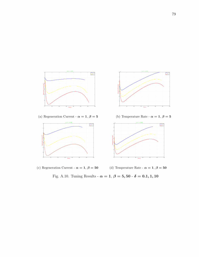
79

0 500 1000 1500 2000 2500 3000 350025

26

27

28

29

30

31

Time (s)

Re

ge

ne

ratio

n C

urr

en

t (A

/m2)

α =1 −− β =5

δ = 0.01

δ = 1

δ = 10

(a) Regeneration Current - α = 1, β = 5

0 500 1000 1500 2000 2500 3000 35002.8

3

3.2

3.4

3.6

3.8

4

4.2x 10

−3

Time (s)

Tem

pera

ture

Rate

(D

eg/s

)

α =1 −− β =5

δ = 0.01

δ = 1

δ = 10

(b) Temperature Rate - α = 1, β = 5

0 500 1000 1500 2000 2500 3000 350025

26

27

28

29

30

31

32

Time (s)

Regenera

tion C

urr

ent (A

/m2)

α =1 −− β =50

δ = 0.01

δ = 1

δ = 10

(c) Regeneration Current - α = 1, β = 50

0 500 1000 1500 2000 2500 3000 35002.8

3

3.2

3.4

3.6

3.8

4

4.2

4.4

4.6x 10

−3

Time (s)

Tem

pera

ture

Rate

(D

eg/s

)

α =1 −− β =50

δ = 0.01

δ = 1

δ = 10

(d) Temperature Rate - α = 1, β = 50

Fig. A.10. Tuning Results - α = 1, β = 5, 50 - δ = 0.1, 1, 10

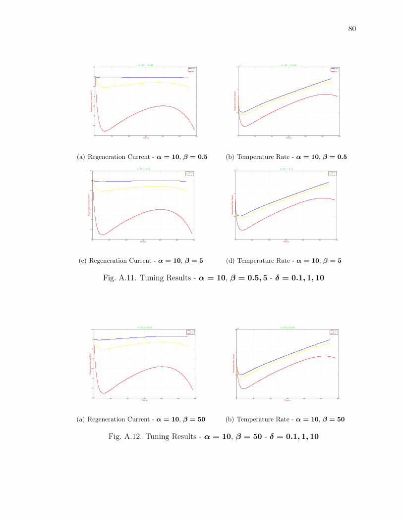
80

0 500 1000 1500 2000 2500 300027

27.5

28

28.5

29

29.5

30

30.5

Time (s)

Regenera

tion C

urr

ent (A

/m2)

α =10 −− β =0.5

δ = 0.01

δ = 1

δ = 10

(a) Regeneration Current - α = 10, β = 0.5

0 500 1000 1500 2000 2500 30003

3.5

4

4.5x 10

−3

Time (s)

Tem

pera

ture

Rate

(D

eg/s

)

α =10 −− β =0.5

δ = 0.01

δ = 1

δ = 10

(b) Temperature Rate - α = 10, β = 0.5

0 500 1000 1500 2000 2500 300027

27.5

28

28.5

29

29.5

30

30.5

Time (s)

Regenera

tion C

urr

ent (A

/m2)

α =10 −− β =5

δ = 0.01

δ = 1

δ = 10

(c) Regeneration Current - α = 10, β = 5

0 500 1000 1500 2000 2500 30003

3.5

4

4.5x 10

−3

Time (s)

Tem

pera

ture

Rate

(D

eg/s

)

α =10 −− β =5

δ = 0.01

δ = 1

δ = 10

(d) Temperature Rate - α = 10, β = 5

Fig. A.11. Tuning Results - α = 10, β = 0.5, 5 - δ = 0.1, 1, 10

0 500 1000 1500 2000 2500 300027

27.5

28

28.5

29

29.5

30

30.5

Time (s)

Regenera

tion C

urr

ent (A

/m2)

α =10 −− β =50

δ = 0.01

δ = 1

δ = 10

(a) Regeneration Current - α = 10, β = 50

0 500 1000 1500 2000 2500 30003

3.5

4

4.5x 10

−3

Time (s)

Tem

pera

ture

Rate

(D

eg/s

)

α =10 −− β =50

δ = 0.01

δ = 1

δ = 10

(b) Temperature Rate - α = 10, β = 50

Fig. A.12. Tuning Results - α = 10, β = 50 - δ = 0.1, 1, 10

81

B. 1-D LITHIUM-ION BATTERY MODEL CODE

************** Battery Model ***************

1D Li Ion Electrochemical Battery Model

***************************************************************

Contents

• Positive Electrode

• Temperature Calculation

• Controller Settings

• Post Processing

% Author :: Sourav Pramanik

% Course :: Master of Science - Thesis

%

% Date :: 20th November 2014

%

% Department :: Mechanical Engineering

%

% Institution :: Indiana University Purdue University Indianapolis

%

% Description :: This is the initialization file for all

% battery parameters and setup configuration.

% Simulation setup information is selected

% from user input.

82

%

% Ce_n, Ce_p, Ce_s are Electrolyte concentrations

% for the Negative, Positive and separator regions.

% They are kept constant at 1000 throughout.

%

% Cs_n, Cs_p are Solid Phase concentration

% qs_n, qs_p are concentration flux

% Css_n, Css_p are surface concentrations

%

% J_n, J_p are molar flux

% Ke_n, Ke_p, Ke_s are ionic conductivity used in

% calculation of Electrolyte potentials

%

% Us_n, Us_p are solid phase potentials

% Ue_n, Ue_p, Ue_s are electrolyte phase potentials

%

% U_eq_n, U_eq_p are over-potentials

% *****************************************************************

clear all;

clc

tic

Li_Ion_1D_Model_Parameter_Determination_Draft09_09_rev2;

% Ce_n,Ce_p,Ce_s are Electrolyte concentrations for the Negative,

% Positive and separator regions. They are kept constant at 1000

% throughout.

83

% Cs_n, Cs_p are Solid Phase concentration

% qs_n, qs_p are concentration flux

% Css_n, Css_p are surface concentrations

% J_n, J_p are molar flux

% Ke_n, Ke_p, Ke_s are ionic conductivity used in calculation of

% Electrolyte potentials

% Us_n, Us_p are solid phase potentials

% Ue_n, Ue_p, Ue_s are electrolyte phase potentials

% U_eq_n, U_eq_p are overpotentials

% ###############################################################

% Equations -

% ###############################################################

%

——— Initial and Boundary Conditions ———-

Applying the initial conditions

---------------------------------------------------------------

Negative Electrode at time t = 0 [Start]

---------------------------------------------------------------

T_n(init_time_node, :) = T_amb;

Ie_n(init_time_node, 1) = 0;

Ie_n(init_time_node, N_n) = I;

% Effective R_eff

84

K_n(init_time_node, 1) = r_eff_n*exp(-30000/R ...

*(1/celltmptr(init_time_node) ...

- 1/T_amb));

% Effective Electrolyte Diffusivity

De_n(init_time_node, 1) = diffu_E_n*exp(-10000/R ...

* (1/celltmptr(init_time_node) ...

- 1/T_amb))*0.21331;

% Electrolyte Concentration is assumed to be constant

Ce_n(init_time_node, 1:N_n) = Ce_init;

% Solid Phase Negative Electrode Concentration

Cs_n(init_time_node, 1:N_n) = stoic_n * Cs_max_n;

Css_n(init_time_node, 1:N_n) = stoic_n * Cs_max_n;

qs_n(init_time_node, 1:N_n) = stoic_n * Cs_max_n;

SOC_n(init_time_node, 1:N_n) = ...

Css_n(init_time_node, 1)/Cs_max_n;

% Electrolyte Conductivity

Ke_n_0(init_time_node, 1:N_n) = ...

(-1.6018e-014) ...

* Ce_n(init_time_node, 1)^4 ...

+ 1.5094e-010*Ce_n(init_time_node, 1)^3 ...

- 4.7212e-007*Ce_n(init_time_node, 1)^2 ...

+ 0.0005007 * Ce_n(init_time_node, 1) ...

+ 0.041253;

% Effective Solid Phase Diffusivity

Ds_n(init_time_node, 1) = diffu_S_n*exp(-20000/R ...

* (1/celltmptr(init_time_node) ...

- 1 / T_amb));

% --------------------------------------------------------------

85

% Separator Region at time t = 0 [Start]

% --------------------------------------------------------------

T_s(init_time_node, :) = T_amb;

Ce_s(init_time_node, 1:N_s) = Ce_init;

Ke_s_0(init_time_node, 1:N_s) = ...

(- 1.6018e-014) ...

* Ce_s(init_time_node, 1)^4 ...

+ 1.5094e-010 * Ce_s(init_time_node, 1)^3 ...

- 4.7212e-007 * Ce_s(init_time_node, 1)^2 ...

+ 0.0005007 * Ce_s(init_time_node, 1) ...

+ 0.041253;

Ie_s(init_time_node, 1:N_s) = I;

% -------------------------------------------------------------

% Positive Electrode at time t = 0 [Start]

% -------------------------------------------------------------

% Effective R_eff

K_p(init_time_node, 1) = r_eff_p*exp(-30000/R ...

* (1/celltmptr(init_time_node) ...

- 1/T_amb));

% Effective Electrolyte Diffusivity

De_p(init_time_node, 1) = diffu_E_p*exp(-10000/R ...

* (1/celltmptr(init_time_node) ...

- 1/T_amb))*0.29585;

% Effective Solid Phase Diffusivity

Ds_p(init_time_node, 1) = diffu_S_p*exp(-4000/R* ...

(1/celltmptr(init_time_node)-1/T_amb));

Ce_p(init_time_node, 1:N_p) = Ce_init;

86

Cs_p(init_time_node, 1:N_p) = stoic_p * Cs_max_p;

Css_p(init_time_node, 1:N_p) = stoic_p * Cs_max_p;

qs_p(init_time_node, 1:N_p) = stoic_p * Cs_max_p;

SOC_p(init_time_node, 1:N_p) = Css_p(init_time_node, 1)/Cs_max_p;

Ke_p_0(init_time_node, 1:N_p) = ...

(- 1.6018e-014) ...

* Ce_p(init_time_node, 1)^4 ...

+ 1.5094e-010 ...

* Ce_p(init_time_node, 1)^3 ...

- 4.7212e-007 ...

* Ce_p(init_time_node, 1)^2 ...

+ 0.0005007 * Ce_p(init_time_node, 1) ...

+ 0.041253;

% -----------------------------------------------------------------

% Negative Electrode

% -----------------------------------------------------------------

J_n(init_time_node, 1) = (I/L_n)*(Rp_n/(3*epss_neg))*(1/F);

Ke_n(init_time_node, 1) = Ke_n_0(init_time_node, 1)*exp(-20000/R* ...

(1/celltmptr(init_time_node)-1/T_amb));

i0_n(init_time_node, 1)= 2 * K_n(init_time_node, 1) ...

* sqrt(Ce_n(init_time_node,1) ...

* (Cs_max_n - Css_n(init_time_node,1)) ...

* Css_n(init_time_node,1));

T_n(init_time_node, 1:N_n) = T_amb;

T_neg(init_time_node, 1:N_n) = T_amb;

eta_neg(init_time_node, 1) = ...

87

((R*celltmptr(init_time_node))/(0.5*F)) ...

*asinh((J_n(init_time_node, 1)) ...

/(i0_n(init_time_node, 1)));

Ue_n(init_time_node, 1) = 0;

if charge == true && mode ~= 3

U_eq_n(init_time_node, 1) = ...

0.15 - 0.10*SOC_n(init_time_node, 1) ...

+ (0.00578/SOC_n(init_time_node, 1));

else

U_eq_n(init_time_node, 1) = ...

0.7222 + 0.1387*SOC_n(init_time_node, 1) ...

+ 0.029*(SOC_n(init_time_node, 1))^0.5 ...

- (0.0172/SOC_n(init_time_node, 1)) ...

+ (0.0019/(SOC_n(init_time_node, 1))^1.5) ...

+ (0.2808*exp(0.90 - 15 ...

* SOC_n(init_time_node, 1))) ...

- (0.7984*exp(0.4465 ...

* SOC_n(init_time_node, 1) - 0.4108));

end

Us_n(init_time_node, 1) = eta_neg(init_time_node, 1) ...

+ Ue_n(init_time_node, 1) ...

+ U_eq_n(init_time_node, 1);

qn_lump(init_time_node, 1) = (3 * epss_neg * F ...

* J_n(init_time_node, 1))/Rp_n ...

* (U_eq_n(init_time_node, 1) ...

- (dudt * celltmptr(init_time_node)));

88

space_node = 2;

while (space_node <= N_n)

K_n(init_time_node, space_node) = ...

r_eff_n * exp(-30000 / R * ...

(1 / celltmptr(init_time_node) ...

- 1/T_amb));

De_n(init_time_node, space_node) = ...

diffu_E_n * exp(-10000/R* ...

(1/celltmptr(init_time_node) ...

- 1/T_amb))*0.21331;

Ds_n(init_time_node, space_node) = ...

diffu_S_n * exp(-20000 / R * ...

(1 / celltmptr(init_time_node) ...

- 1/T_amb));

if space_node ~= N_n

Ie_n(init_time_node, space_node) = ...

((3*epss_neg ...

* J_n(init_time_node, space_node-1) ...

* F*grid_n)/Rp_n) ...

+ Ie_n(init_time_node, space_node-1);

end

Us_n(init_time_node, space_node) = ...

((Ie_n(init_time_node, space_node-1) - I)/sigma_n) ...

89

* grid_n + Us_n(init_time_node, space_node-1);

Ke_n(init_time_node, space_node) = ...

Ke_n_0(init_time_node, space_node)*exp(-20000/R* ...

(1/celltmptr(init_time_node)-1/T_amb));

Ue_n(init_time_node, space_node) = ...

(-Ie_n(init_time_node, space_node-1) ...

/ Ke_n(init_time_node, space_node)*grid_n) ...

+ Ue_n(init_time_node, space_node-1);

if charge == true && mode ~= 3

U_eq_n(init_time_node, space_node) = ...

0.15 - 0.10*SOC_n(init_time_node, space_node) ...

+ (0.00578/SOC_n(init_time_node, space_node));

else

U_eq_n(init_time_node, space_node) = ...

0.7222 + 0.1387*SOC_n(init_time_node, space_node) ...

+0.029*(SOC_n(init_time_node, space_node))^0.5 ...

-(0.0172/SOC_n(init_time_node, space_node)) ...

+(0.0019/(SOC_n(init_time_node, space_node))^1.5) ...

+(0.2808*exp(0.90 - 15 ...

*SOC_n(init_time_node, space_node))) ...

-(0.7984*exp(0.4465*SOC_n(init_time_node, space_node) ...

-0.4108));

end

eta_neg(init_time_node, space_node) = ...

Us_n(init_time_node, space_node) ...

90

- Ue_n(init_time_node, space_node) ...

- U_eq_n(init_time_node, space_node);

i0_n(init_time_node, space_node) = ...

2 * K_n(init_time_node, space_node) ...

* sqrt(Ce_n(init_time_node,space_node) ...

* (Cs_max_n - Css_n(init_time_node, space_node)) ...

* Css_n(init_time_node, space_node));

J_n(init_time_node, space_node) = ...

i0_n(init_time_node, space_node) ...

* sinh((0.5*F*eta_neg(init_time_node, space_node)) ...

/(R*celltmptr(init_time_node)));

q_n(init_time_node, space_node) = ...

i_app*23.7*(-(3*epss_neg * F ...

* J_n(init_time_node, space_node))/Rp_n ...

* (eta_neg(init_time_node, space_node) ...

- dudt * celltmptr(init_time_node)));

qn_lump(init_time_node, space_node) = ...

(3*epss_neg*F*J_n(init_time_node, space_node))/Rp_n ...

* (U_eq_n(init_time_node, space_node) ...

- (dudt * celltmptr(init_time_node)));

space_node = space_node + 1;

end

% Separator Region

91

De_s(init_time_node, 1) = ...

diffu_E_s * exp(-10000 / R * ...

(1 / celltmptr(init_time_node) - 1/T_amb));

Ke_s(init_time_node, 1) = ...

Ke_s_0(init_time_node, 1) * exp(-20000 / R ...

* (1 / celltmptr(init_time_node) - 1/T_amb));

T_s(init_time_node, 1:N_s) = T_amb;

Ue_s(init_time_node, 1) = Ue_n(init_time_node, N_n);

space_node = 2;

while (space_node < N_s)

De_s(init_time_node, space_node) = ...

diffu_E_s * exp(-10000 / R * ...

(1 / celltmptr(init_time_node) ...

- 1/T_amb));

Ke_s(init_time_node, space_node) = ...

Ke_s_0(init_time_node, space_node) ...

* exp(-20000/R*(1/celltmptr(init_time_node)-1/T_amb));

Ue_s(init_time_node, space_node) = ...

(-Ie_s(init_time_node, space_node-1) ...

/Ke_s(init_time_node, space_node) + ...

(2*R*celltmptr(init_time_node)*(1-t_plus) ...

*(log(Ce_s(init_time_node,space_node)) ...

- log(Ce_s(init_time_node,space_node-1))) ...

/(F*grid_s)))*grid_s ...

+ Ue_s(init_time_node, space_node-1);

92

space_node = space_node + 1;

end

De_s(init_time_node, N_s) = ...

diffu_E_s * exp(-10000 / R * ...

(1 / celltmptr(init_time_node) - 1 / T_amb));

Ue_s(init_time_node, N_s) = ...

(-Ie_s(init_time_node, N_s - 1) ...

/ Ke_n(init_time_node, N_n) + ...

(2*R*celltmptr(init_time_node)*(1-t_plus) ...

*(log(Ce_s(init_time_node,N_s)) ...

- log(Ce_s(init_time_node,N_s-1))) ...

/(F*grid_s))) ...

* grid_s + Ue_s(init_time_node, N_s-1);

%

Positive Electrode

T_p(init_time_node, :) = T_amb;

T_p(init_time_node, 1:N_p) = T_amb;

Ue_p(init_time_node, 1) = 0;

Ie_p(init_time_node, 1) = 0;

Ie_p(init_time_node, N_p) = -I;

Ke_p(init_time_node, 1) = ...

Ke_p_0(init_time_node, 1) ...

93

* exp(-20000 / R ...

* (1 / celltmptr(init_time_node) ...

- 1 / T_amb));

J_p(init_time_node, 1) = -(I/L_p)*(Rp_p/(3*epss_pos))*(1/F);

i0_p(init_time_node, 1)= ...

2 * K_p(init_time_node, 1) ...

* sqrt(Ce_p(init_time_node,1)...

* (Cs_max_p - Css_p(init_time_node,1)) ...

* Css_p(init_time_node,1));

eta_pos(init_time_node, 1) = ((R*celltmptr(init_time_node)) ...

/ (0.5*F)) ...

* asinh((J_p(init_time_node, 1)) ...

/ (i0_p(init_time_node, 1)));

if charge == true && mode ~= 3

U_eq_p(init_time_node, 1) = ...

(-4.875 + (5.839*SOC_p(init_time_node, 1)) ...

- (1.507*SOC_p(init_time_node, 1)^3) ...

+ (0.533*SOC_p(init_time_node, 1)^5)) ...

/ (SOC_p(init_time_node, 1) - 1.03);

else

U_eq_p(init_time_node, 1) = ...

(-4.656+ 88.669*(SOC_p(init_time_node, 1))^2 ...

- 401.119*(SOC_p(init_time_node, 1))^4 ...

+ 342.909*(SOC_p(init_time_node, 1))^6 ...

- 462.471*(SOC_p(init_time_node, 1))^8 ...

+ 433.434*(SOC_p(init_time_node, 1))^10)/...

94

(-1.0+18.933*(SOC_p(init_time_node, 1))^2 ...

- 79.532*(SOC_p(init_time_node, 1))^4 ...

+ 37.311*(SOC_p(init_time_node, 1))^6 ...

- 73.083*(SOC_p(init_time_node, 1))^8 ...

+ 95.96*(SOC_p(init_time_node, 1))^10);

end

Us_p(init_time_node, 1) = eta_pos(init_time_node, 1) ...

+ Ue_p(init_time_node, 1) ...

+ U_eq_p(init_time_node, 1);

q_p(init_time_node, 1) = i_app*23.7*(-(3*epss_pos * F ...

* J_p(init_time_node, 1))/Rp_p ...

* (eta_pos(init_time_node, 1) ...

- dudt*celltmptr(init_time_node)) ...

- Ue_p(init_time_node, 1) ...

* Ie_p(init_time_node, 1) ...

+ Us_p(init_time_node, 1) ...

*(I - Ie_p(init_time_node, 1)));

qp_lump(init_time_node, 1) = (3 * epss_pos * F ...

* J_p(init_time_node, 1))/Rp_p ...

* (U_eq_p(init_time_node, 1) ...

- (dudt * celltmptr(init_time_node)));

space_node = 2;

while (space_node <= N_p)

K_p(init_time_node, space_node) = ...

r_eff_p*exp(-30000/R ...

* (1/celltmptr(init_time_node) ...

95

- 1/T_amb));

De_p(init_time_node, space_node) = ...

diffu_E_p * exp(-10000 / R ...

*(1/celltmptr(init_time_node) ...

-1/T_amb))*0.29585;

Ds_p(init_time_node, space_node) = ...

diffu_S_p * exp(-4000 / R ...

* (1 / celltmptr(init_time_node) ...

- 1 / T_amb));

if space_node ~= N_p

Ie_p(init_time_node, space_node) = ...

((3*epss_pos*J_p(init_time_node, space_node - 1) ...

* F*grid_p)/Rp_p) ...

+ Ie_p(init_time_node, space_node - 1);

end

Us_p(init_time_node, space_node) = ...

((Ie_p(init_time_node, space_node - 1) ...

- I)/sigma_p)*grid_p ...

+ Us_p(init_time_node, space_node - 1);

Ke_p(init_time_node, space_node) = ...

Ke_p_0(init_time_node, space_node) ...

* exp(-20000 / R * (1 / celltmptr(init_time_node) ...

- 1 / T_amb));

Ue_p(init_time_node, space_node) = ...

96

(-Ie_p(init_time_node, space_node-1) ...

/ Ke_p(init_time_node, space_node))*grid_p ...

+ Ue_p(init_time_node, space_node-1);

if charge == true && mode ~= 3

U_eq_p(init_time_node, space_node) = ...

(-4.875 + (5.839*SOC_p(init_time_node, space_node)) ...

- (1.507*SOC_p(init_time_node, space_node)^3) ...

+ (0.533*SOC_p(init_time_node, space_node)^5)) ...

/(SOC_p(init_time_node, space_node) - 1.03);

else

U_eq_p(init_time_node, space_node) = ...

(-4.656+ 88.669*(SOC_p(init_time_node, space_node))^2 ...

- 401.119*(SOC_p(init_time_node,space_node))^4 ...

+ 342.909*(SOC_p(init_time_node, space_node))^6 ...

- 462.471*(SOC_p(init_time_node, space_node))^8 ...

+ 433.434*(SOC_p(init_time_node, space_node))^10)/...

(-1.0+18.933*(SOC_p(init_time_node, space_node))^2 ...

- 79.532*(SOC_p(init_time_node, space_node))^4 ...

+ 37.311*(SOC_p(init_time_node, space_node))^6 ...

- 73.083*(SOC_p(init_time_node, space_node))^8 ...

+ 95.96*(SOC_p(init_time_node, space_node))^10);

end

eta_pos(init_time_node, space_node) = ...

Us_p(init_time_node, space_node) ...

- Ue_p(init_time_node, space_node) ...

- U_eq_p(init_time_node, space_node);

97

i0_p(init_time_node, space_node) = ...

2 * K_p(init_time_node, space_node) ...

* sqrt(Ce_p(init_time_node,space_node) ...

* (Cs_max_p - Css_p(init_time_node, space_node)) ...

* Css_p(init_time_node, space_node));

J_p(init_time_node, space_node) = ...

i0_p(init_time_node, space_node) ...

* sinh((0.5*F*eta_pos(init_time_node, space_node)) ...

/ (R*celltmptr(init_time_node)));

q_p(init_time_node, space_node) = ...

i_app*23.7*(-(3*epss_pos * F ...

* J_p(init_time_node, space_node)) ...

/ Rp_p * (eta_pos(init_time_node, space_node) ...

- dudt*celltmptr(init_time_node)) ...

- Ue_p(init_time_node, space_node) ...

* Ie_p(init_time_node, space_node) ...

+ Us_p(init_time_node, space_node) ...

* (I - Ie_p(init_time_node, space_node)));

qp_lump(init_time_node, space_node) = ...

(3 * epss_pos * F ...

* J_p(init_time_node, space_node))/Rp_p ...

* (U_eq_p(init_time_node, space_node) ...

- (dudt * celltmptr(init_time_node)));

space_node = space_node + 1;

end

init_soc = SOC_n(init_time_node,1);

98

count = 1;

Voltage(init_time_node) = Us_p(init_time_node, 1) ...

- Us_n(init_time_node, 1);

Current(init_time_node) = I;

if charge == true

Q(count) = -I*dt;

SOC(count) = (Q(count)/(R_Cap)) + init_soc;

else

Q(count) = I*dt;

SOC(count) = init_soc - (Q(count)/(R_Cap));

end

count = count + 1;

ocp(init_time_node) = U_eq_p(init_time_node, 1) ...

- U_eq_n(init_time_node, 1);

Cs_n_avg(init_time_node) = sum(Cs_n(init_time_node,:))/N_n;

SOC_Cs(init_time_node) = Cs_n_avg(init_time_node)/Cs_max_n;

if mode == 4

delta(init_time_node) = ...

((alpha_ac*F*sum(eta_neg(init_time_node,:))/N_n) ...

/(R*celltmptr(init_time_node)^2)) ...

* ((6*sum(i0_n(init_time_node,:))/N_n)/(R*F)) ...

* cosh((alpha_ac*F*sum(eta_neg(init_time_node,:))/N_n) ...

/(R*celltmptr(init_time_node)));

gamma(init_time_node) = ...

((3*epss_neg*F*dudt*sum(J_n(init_time_node,:))/Rp_n) ...

+ (3*epss_pos*F*dudt*sum(J_p(init_time_node,:)) ...

99

/Rp_p))/rho_cp_avg;

lambda_2(init_time_node) = ...

(-I*(1+(2*alpha))+(2*alpha*I_max)) ...

* rho_cp_avg/Voltage(init_time_node);

lambda_1(init_time_node) = ...

((I*(1+(2*alpha))) - (2*alpha*I_max) ...

+ (lambda_2(init_time_node) ...

* Voltage(init_time_node) ...

/ rho_cp_avg)) * zeta;

end

celltmptr_rate(init_time_node) = 0;

Iterative Equations

% This is time iteration from second time step onwards.

% In each time step the space nodes are iterated.

for time_node = 2:max_time

% Calculations for Negative Electrode

% **********************************************************

% Inner iteration within each time step to reach convergence

% Boundary Values - Negative

Ie_n(time_node, 1) = 0;

Ie_n(time_node, N_n) = I;

J_n(time_node, 1) = (I/L_n)*(Rp_n/(3*epss_neg))*(1/F);

100

K_n(time_node, 1) = r_eff_n * exp(-30000 / R ...

* (1 / celltmptr(time_node - 1) ...

- 1 / T_amb));

De_n(time_node, 1) = diffu_E_n * exp(-10000/R ...

* (1/celltmptr(time_node-1) ...

- 1/T_amb))*0.21331;

Ce_n(time_node, 1) = Ce_init;

Cs_n(time_node, 1) = ((-3/Rp_n)*J_n(time_node - 1, 1) * dt) ...

+ Cs_n(time_node - 1, 1);

Ds_n(time_node, 1) = diffu_S_n * exp(-20000 / R ...

* (1 / celltmptr(time_node-1) ...

- 1 / T_amb));

qs_n(time_node, 1) = ...

-(((30*Ds_n(time_node, 1))/Rp_n^2) ...

* qs_n(time_node-1, 1)*dt) ...

- ((45/(2*Rp_n^2))*J_n(time_node-1, 1)*dt) ...

+ qs_n(time_node-1, 1);

Css_n(time_node, 1) = ...

Cs_n(time_node, 1 ) ...

+(((8*Rp_n)/35)*qs_n(time_node, 1)) ...

-((Rp_n/(35*Ds_n(time_node, 1)))*J_n(time_node-1, 1));

SOC_n(time_node, 1) =Css_n(time_node, 1)/Cs_max_n;

101

Ke_n_0(time_node, 1)=(- 1.6018e-014)*Ce_n(time_node, 1)^4 ...

+ 1.5094e-010*Ce_n(time_node, 1)^3 ...

- 4.7212e-007 * Ce_n(time_node, 1)^2 ...

+ 0.0005007*Ce_n(time_node, 1)+0.041253;

Ke_n(time_node, 1) = Ke_n_0(time_node,1) * exp(-20000/R ...

*(1/celltmptr(time_node-1)-1/T_amb));

i0_n(time_node, 1) = 2 * K_n(time_node, 1) ...

* sqrt(Ce_n(time_node,1) ...

*(Cs_max_n - Css_n(time_node, 1)) ...

* Css_n(time_node, 1));

eta_neg(time_node, 1) = ((R*celltmptr(time_node-1))/(0.5*F)) ...

* asinh((J_n(time_node-1, 1)) ...

/(i0_n(time_node, 1)));

Ue_n(time_node, 1) = 0;

if charge == true && mode ~= 3

U_eq_n(time_node, 1) = 0.15 - 0.10*SOC_n(time_node, 1) ...

+ (0.00578/SOC_n(time_node, 1));

else

U_eq_n(time_node, 1) = ...

0.7222 + 0.1387*SOC_n(time_node, 1) ...

+ 0.029*(SOC_n(time_node, 1))^0.5 ...

- (0.0172/SOC_n(time_node, 1)) ...

+ (0.0019/(SOC_n(time_node, 1))^1.5) ...

+ (0.2808*exp(0.90 - 15*SOC_n(time_node, 1))) ...

102

- (0.7984*exp(0.4465*SOC_n(time_node, 1) ...

- 0.4108));

end

Us_n(time_node, 1) = eta_neg(time_node, 1) ...

+ Ue_n(time_node, 1) ...

+ U_eq_n(time_node, 1);

q_n(time_node, 1) = i_app*22.3*(-(3*epss_neg * F ...

* J_n(time_node, 1))/Rp_n ...

* (eta_neg(time_node, 1) ...

- dudt*celltmptr(time_node-1)));

qn_lump(time_node, 1) = (3 * epss_neg * F ...

* J_n(time_node, 1))/Rp_n ...

* (U_eq_n(time_node, 1) ...

- (dudt * celltmptr(time_node - 1)));

% Looping in Internal Space Nodes

for space_node = 2:N_n

% Ionic Current in Negative Electrode

if space_node ~= N_n

Ie_n(time_node, space_node) = ...

((3*epss_neg * J_n(time_node, space_node-1) ...

* F*grid_n)/Rp_n) ...

+ Ie_n(time_node, space_node-1);

end

103

De_n(time_node, space_node) = diffu_E_n * exp(-10000/R ...

*(1/celltmptr(time_node-1) ...

-1/T_amb))*0.21331;

if space_node ~= N_n

Ce_n(time_node, space_node) = ...

((De_n(time_node - 1, space_node)) ...

*((Ce_n(time_node - 1,space_node + 1) ...

- 2*Ce_n(time_node-1, space_node) ...

+ Ce_n(time_node-1, space_node - 1))/grid_n^2) + ...

(t_plus*(Ie_n(time_node-1, space_node) ...

- Ie_n(time_node - 1,space_node-1)) ...

/(grid_n*F)))*dt ...

+ Ce_n(time_node - 1, space_node);

else

Ce_n(time_node, space_node) = (4/3)*Ce_n(time_node, N_n - 1) ...

- (1/3) * Ce_n(time_node, N_n - 2);

end

% Li+ Concentration in Negative Electrode

Cs_n(time_node, space_node) = ...

((-3/Rp_n)*J_n(time_node-1, space_node)*dt) ...

+ Cs_n(time_node-1, space_node);

Ds_n(time_node, space_node) = diffu_S_n * exp(-20000 / R ...

* (1 / celltmptr(time_node-1) ...

- 1 / T_amb));

104

% Li+ Concentration Flux in Negative Electrode

qs_n(time_node, space_node) = ...

-(((30*Ds_n(time_node, space_node))/Rp_n^2) ...

* qs_n(time_node-1, space_node)*dt) ...

- ((45/(2*Rp_n^2)) ...

* J_n(time_node-1, space_node)*dt) ...

+ qs_n(time_node-1, space_node);

% Li+ Solid/Electrolyte Concentration in Negative Electrode

Css_n(time_node, space_node) = ...

Cs_n(time_node, space_node) ...

+ (((8*Rp_n)/35) ...

* qs_n(time_node, space_node)) ...

- ((Rp_n/(35*Ds_n(time_node, space_node))) ...

* J_n(time_node, space_node-1));

% State of Charge in Negative Electrode

SOC_n(time_node, space_node) = ...

Css_n(time_node, space_node)/Cs_max_n;

% Solid Phase Potential in Negative Electrode

Us_n(time_node, space_node) = ...

((Ie_n(time_node, space_node-1) ...

- I)/sigma_n)*grid_n ...

+ Us_n(time_node, space_node-1);

Ke_n_0(time_node, space_node) = ...

(-1.6018e-014) * Ce_n(time_node, space_node)^4 ...

105

+ 1.5094e-010 * Ce_n(time_node, space_node)^3 ...

- 4.7212e-007 * Ce_n(time_node, space_node)^2 ...

+ 0.0005007 * Ce_n(time_node, space_node) + 0.041253;

Ke_n(time_node, space_node) = Ke_n_0(time_node, space_node) ...

* exp(-20000/R ...

* (1/celltmptr(time_node-1)...

-1/T_amb));

Ue_n(time_node, space_node) = ...

((-Ie_n(time_node, space_node-1) ...

/ Ke_n(time_node, space_node)) ...

+ (2*R*celltmptr(time_node-1)*(1-t_plus) ...

* (log(Ce_n(time_node,space_node)) ...

- log(Ce_n(time_node,space_node - 1))) ...

/(F*grid_n)))*grid_n ...

+ Ue_n(time_node, space_node-1);

% Over-potential Calculation

if charge == true && mode ~= 3

U_eq_n(time_node, space_node) = ...

0.15 - 0.10*SOC_n(time_node, space_node) ...

+ (0.00578/SOC_n(time_node, space_node));

else

U_eq_n(time_node, space_node) = ...

0.7222 + 0.1387*SOC_n(time_node, space_node) ...

+ 0.029*(SOC_n(time_node, space_node))^0.5 ...

- (0.0172/SOC_n(time_node, space_node)) ...

+ (0.0019/(SOC_n(time_node, space_node))^1.5) ...

106

+ (0.2808*exp(0.90 - 15 ...

* SOC_n(time_node, space_node))) ...

- (0.7984*exp(0.4465 ...

* SOC_n(time_node, space_node) - 0.4108));

end

eta_neg(time_node, space_node) = ...

Us_n(time_node, space_node) ...

- Ue_n(time_node, space_node) ...

- U_eq_n(time_node, space_node);

% Molar Ionic Flux [UNIT: A/m^2]

K_n(time_node, space_node) = r_eff_n * exp(-30000/R ...

*(1/celltmptr(time_node-1)-1/T_amb));

i0_n(time_node, space_node) = ...

2 * K_n(time_node, space_node) ...

* sqrt(Ce_n(time_node,space_node) ...

* (Cs_max_n - Css_n(time_node, space_node)) ...

* Css_n(time_node, space_node));

J_n(time_node, space_node) = ...

i0_n(time_node, space_node) ...

* sinh((0.5*F*eta_neg(time_node, space_node)) ...

/(R*celltmptr(time_node - 1)));

q_n(time_node, space_node) = i_app*22.3*(-(3*epss_neg * F ...

* J_n(time_node, space_node))/Rp_n ...

* (eta_neg(time_node, space_node) ...

107

- dudt*celltmptr(time_node-1)));

qn_lump(time_node, space_node) = ...

(3 * epss_neg * F ...

* J_n(time_node, space_node))/Rp_n ...

* (U_eq_n(time_node, space_node) ...

- (dudt * celltmptr(time_node - 1)));

end

% ###############################################################

********* Calculation of Separator Region Parameters ************

% Boundary Condition Setup

De_s(time_node, 1) = diffu_E_s * exp(-10000 / R ...

* (1 / celltmptr(time_node-1) - 1 / T_amb));

Ue_s(time_node, 1) = Ue_n(time_node, N_n);

Ce_s(time_node, 1) = Ce_s(time_node - 1, 2)...

-((De_n(time_node, 1) ...

* grid_s/De_s(time_node,1))...

*(Ce_n(time_node, N_n) ...

- Ce_n(time_node, N_n-1))/grid_n);

q_s(time_node, 1) = 0;

Ke_s_0(time_node, 1) = (-1.6018e-014) * Ce_s(time_node, 1)^4 ...

+ 1.5094e-010 * Ce_s(time_node, 1)^3 ...

- 4.7212e-007 * Ce_s(time_node, 1)^2 ...

+ 0.0005007*Ce_s(time_node, 1) + 0.041253;

108

Ke_s(time_node, 1) = Ke_s_0(time_node, 1) * exp(-20000/R ...

* (1/celltmptr(time_node-1)-1/T_amb));

Ie_s(time_node, :) = I;

% Looping in internal Space nodes

for space_node = 2:N_s - 1

De_s(time_node, space_node) = diffu_E_s * exp(-10000 / R ...

* (1 / celltmptr(time_node-1) ...

- 1 / T_amb));

Ce_s(time_node, space_node) = ...

((De_s(time_node-1, space_node) ...

* (Ce_s(time_node-1,space_node+1) ...

- 2*Ce_s(time_node-1, space_node) ...

+ Ce_s(time_node-1, space_node-1))/grid_s^2))*dt ...

+ Ce_s(time_node - 1, space_node);

% Electrolyte Phase Potential

Ke_s_0(time_node, space_node) = ...

(-1.6018e-014) * Ce_s(time_node, space_node)^4 ...

+ 1.5094e-010 * Ce_s(time_node, space_node)^3 ...

- 4.7212e-007 * Ce_s(time_node, space_node)^2 ...

+ 0.0005007 * Ce_s(time_node, space_node) ...

+ 0.041253;

Ke_s(time_node, space_node) = Ke_s_0(time_node, space_node) ...

* exp(-20000/R ...

*(1/celltmptr(time_node-1)-1/T_amb));

109

Ue_s(time_node, space_node) = ...

(-I/Ke_s(time_node, space_node) + ...

(2*R*celltmptr(time_node-1)*(1-t_plus) ...

*(log(Ce_s(time_node,space_node)) ...

- log(Ce_s(time_node,space_node-1))) ...

/(F*grid_s)))*grid_s ...

+ Ue_s(time_node, space_node-1);

q_s(time_node, space_node) = ...

-i_app*23.7*I*Ue_s(time_node, space_node);

end

% Boundary Condition Setup

De_s(time_node, N_s) = diffu_E_s * exp(-10000/R ...

*(1/celltmptr(time_node-1)-1/T_amb));

Ce_s(time_node, N_s) = Ce_s(time_node - 1, N_s-1) ...

+ ((De_p(time_node-1, N_p) ...

* grid_s/De_s(time_node,N_s)) ...

* (Ce_n(time_node, N_p) ...

- Ce_n(time_node, N_p-1))/grid_p);

Ke_s_0(time_node, N_s) = ...

(-1.6018e-014) * Ce_s(time_node, N_s)^4 ...

+ 1.5094e-010*Ce_s(time_node, N_s)^3 ...

- 4.7212e-007 * Ce_s(time_node, N_s)^2 ...

+ 0.0005007 * Ce_s(time_node, N_s) ...

110

+ 0.041253;

Ke_s(time_node, N_s) = Ke_s_0(time_node, N_s) ...

* exp(-20000/R ...

* (1/celltmptr(time_node-1)-1/T_amb));

Ue_s(time_node, N_s) = ...

(-I/Ke_s(time_node, N_s) + ...

(2*R*celltmptr(time_node-1)*(1-t_plus) ...

* (log(Ce_s(time_node,N_s)) ...

- log(Ce_s(time_node,N_s-1))) ...

/(F*grid_s)))*grid_s ...

+ Ue_s(time_node, N_s-1);

q_s(time_node, N_s) = -i_app*23.7*I*Ue_s(time_node, N_s);

% #######################################################

********* Calculations for Positive Electrode *********** *Calculation is done from

extreme positive end towards separator* ************* Boundary Values - Positive

*************

Ue_p(time_node, 1) = 0;

Ie_p(time_node, 1) = 0;

Ie_p(time_node, N_p) = -I;

J_p(time_node, 1) = -(I/L_p)*(Rp_p/(3*epss_pos))*(1/F);

Ce_p(time_node, 1) = Ce_init;

if charge == true

Ce_p(time_node, 1) = min(Ce_Hi_lim,Ce_p(time_node, 1));

else

111

Ce_p(time_node, 1) = max(Ce_Lo_lim,Ce_p(time_node, 1));

end

De_p(time_node, 1) = diffu_E_p * exp(-10000/R ...

* (1/celltmptr(time_node-1) ...

- 1/T_amb))*0.29585;

Ds_p(time_node, 1) = diffu_S_p * exp(-4000/R ...

* (1/celltmptr(time_node-1) ...

- 1/T_amb));

Cs_p(time_node, 1) = ((-3/Rp_p)*J_p(time_node-1, 1)*dt) ...

+ Cs_p(time_node-1, 1);

qs_p(time_node, 1) = -(((30*Ds_p(time_node, 1))/Rp_p^2) ...

* qs_p(time_node-1, 1)*dt) ...

- ((45/(2*Rp_p^2)) ...

* J_p(time_node-1, 1)*dt) ...

+ qs_p(time_node-1, 1);

Css_p(time_node, 1) = Cs_p(time_node-1, 1) ...

+ (((8*Rp_p)/35) ...

* qs_p(time_node-1, 1)) ...

- ((Rp_p/(35*Ds_p(time_node, 1))) ...

* J_p(time_node-1, 1));

SOC_p(time_node, 1) = Css_p(time_node, 1)/Cs_max_p;

K_p(time_node, 1) = r_eff_p * exp(-30000 / R ...

* (1 / celltmptr(time_node-1) ...

112

- 1 / T_amb));

i0_p(time_node, 1) = 2 * K_p(time_node, 1) ...

* sqrt(Ce_p(time_node,1) ...

* (Cs_max_p - Css_p(time_node, 1)) ...

* Css_p(time_node, 1));

eta_pos(time_node, 1) = R*celltmptr(time_node-1)/(0.5*F) ...

* asinh((J_p(time_node-1, 1)) ...

/(i0_p(time_node, 1)));

if charge == true && mode ~= 3

U_eq_p(time_node, 1) = (-4.875 + (5.8399*SOC_p(time_node, 1)) ...

- (1.507*SOC_p(time_node, 1)^3) ...

+ (0.533*SOC_p(time_node, 1)^5)) ...

/(SOC_p(time_node, 1) - 1.03);

else

U_eq_p(time_node, 1) = ...

(-4.656 + 88.669*(SOC_p(time_node, 1))^2 ...

- 401.119*(SOC_p(time_node,1))^4 ...

+ 342.909*(SOC_p(time_node, 1))^6 ...

- 462.471*(SOC_p(time_node, 1))^8 ...

+ 433.434*(SOC_p(time_node, 1))^10)/...

(- 1.0+18.933*(SOC_p(time_node, 1))^2 ...

- 79.532*(SOC_p(time_node, 1))^4 ...

+ 37.311*(SOC_p(time_node, 1))^6 ...

- 73.083*(SOC_p(time_node, 1))^8 ...

+ 95.96*(SOC_p(time_node, 1))^10);

end

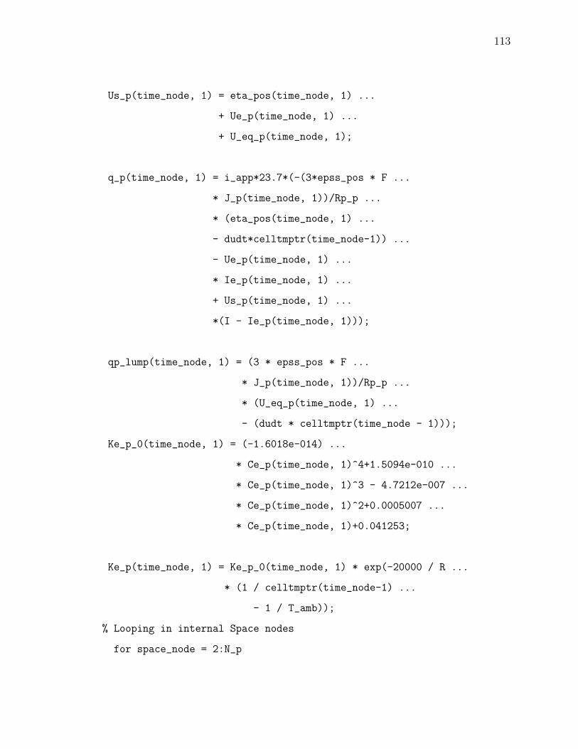
113

Us_p(time_node, 1) = eta_pos(time_node, 1) ...

+ Ue_p(time_node, 1) ...

+ U_eq_p(time_node, 1);

q_p(time_node, 1) = i_app*23.7*(-(3*epss_pos * F ...

* J_p(time_node, 1))/Rp_p ...

* (eta_pos(time_node, 1) ...

- dudt*celltmptr(time_node-1)) ...

- Ue_p(time_node, 1) ...

* Ie_p(time_node, 1) ...

+ Us_p(time_node, 1) ...

*(I - Ie_p(time_node, 1)));

qp_lump(time_node, 1) = (3 * epss_pos * F ...

* J_p(time_node, 1))/Rp_p ...

* (U_eq_p(time_node, 1) ...

- (dudt * celltmptr(time_node - 1)));

Ke_p_0(time_node, 1) = (-1.6018e-014) ...

* Ce_p(time_node, 1)^4+1.5094e-010 ...

* Ce_p(time_node, 1)^3 - 4.7212e-007 ...

* Ce_p(time_node, 1)^2+0.0005007 ...

* Ce_p(time_node, 1)+0.041253;

Ke_p(time_node, 1) = Ke_p_0(time_node, 1) * exp(-20000 / R ...

* (1 / celltmptr(time_node-1) ...

- 1 / T_amb));

% Looping in internal Space nodes

for space_node = 2:N_p

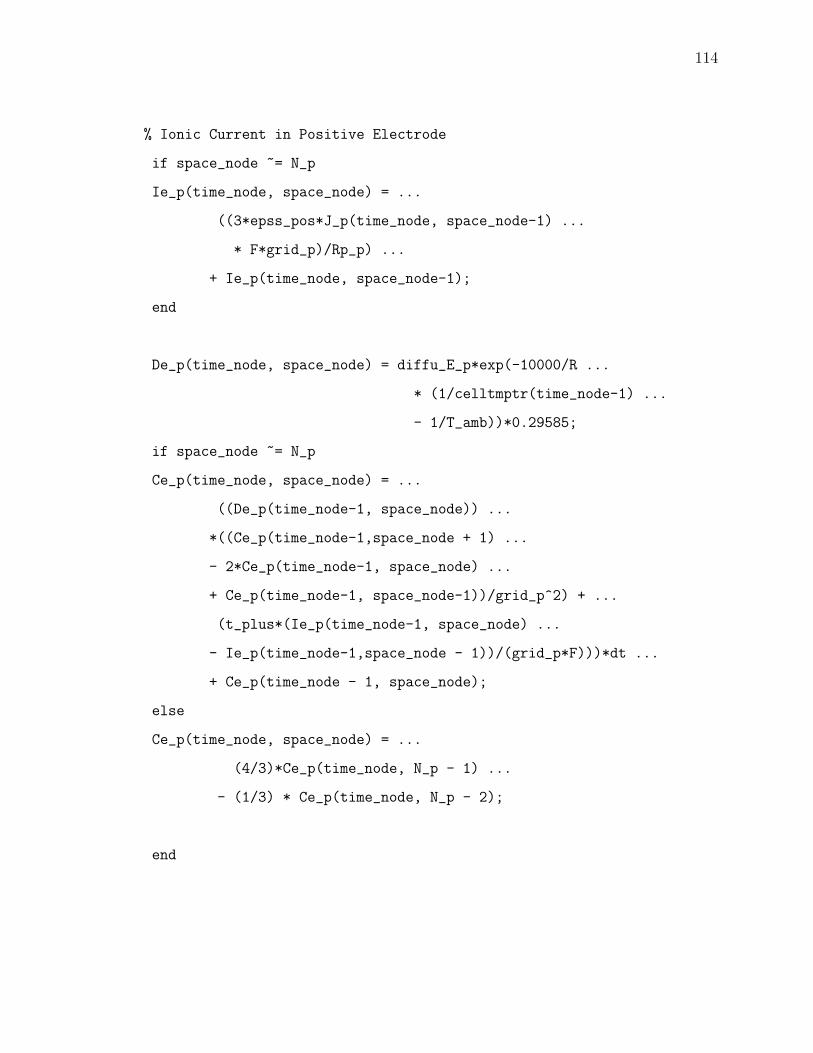
114

% Ionic Current in Positive Electrode

if space_node ~= N_p

Ie_p(time_node, space_node) = ...

((3*epss_pos*J_p(time_node, space_node-1) ...

* F*grid_p)/Rp_p) ...

+ Ie_p(time_node, space_node-1);

end

De_p(time_node, space_node) = diffu_E_p*exp(-10000/R ...

* (1/celltmptr(time_node-1) ...

- 1/T_amb))*0.29585;

if space_node ~= N_p

Ce_p(time_node, space_node) = ...

((De_p(time_node-1, space_node)) ...

*((Ce_p(time_node-1,space_node + 1) ...

- 2*Ce_p(time_node-1, space_node) ...

+ Ce_p(time_node-1, space_node-1))/grid_p^2) + ...

(t_plus*(Ie_p(time_node-1, space_node) ...

- Ie_p(time_node-1,space_node - 1))/(grid_p*F)))*dt ...

+ Ce_p(time_node - 1, space_node);

else

Ce_p(time_node, space_node) = ...

(4/3)*Ce_p(time_node, N_p - 1) ...

- (1/3) * Ce_p(time_node, N_p - 2);

end

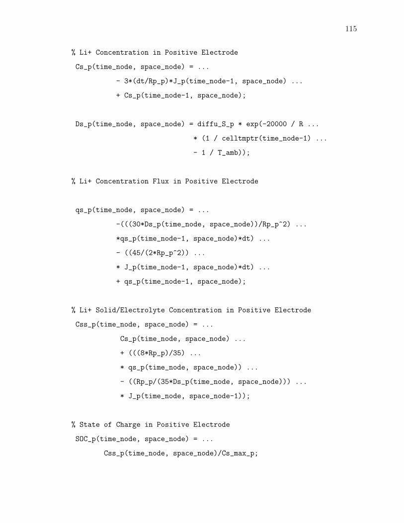
115

% Li+ Concentration in Positive Electrode

Cs_p(time_node, space_node) = ...

- 3*(dt/Rp_p)*J_p(time_node-1, space_node) ...

+ Cs_p(time_node-1, space_node);

Ds_p(time_node, space_node) = diffu_S_p * exp(-20000 / R ...

* (1 / celltmptr(time_node-1) ...

- 1 / T_amb));

% Li+ Concentration Flux in Positive Electrode

qs_p(time_node, space_node) = ...

-(((30*Ds_p(time_node, space_node))/Rp_p^2) ...

*qs_p(time_node-1, space_node)*dt) ...

- ((45/(2*Rp_p^2)) ...

* J_p(time_node-1, space_node)*dt) ...

+ qs_p(time_node-1, space_node);

% Li+ Solid/Electrolyte Concentration in Positive Electrode

Css_p(time_node, space_node) = ...

Cs_p(time_node, space_node) ...

+ (((8*Rp_p)/35) ...

* qs_p(time_node, space_node)) ...

- ((Rp_p/(35*Ds_p(time_node, space_node))) ...

* J_p(time_node, space_node-1));

% State of Charge in Positive Electrode

SOC_p(time_node, space_node) = ...

Css_p(time_node, space_node)/Cs_max_p;

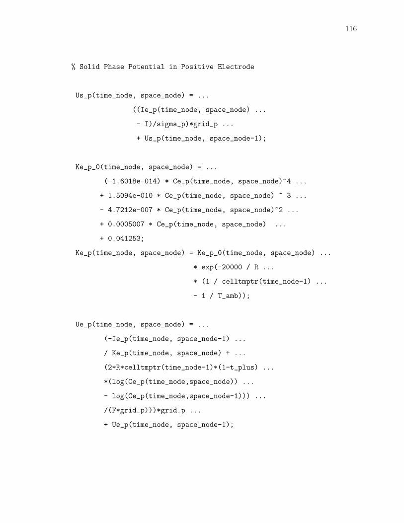
116

% Solid Phase Potential in Positive Electrode

Us_p(time_node, space_node) = ...

((Ie_p(time_node, space_node) ...

- I)/sigma_p)*grid_p ...

+ Us_p(time_node, space_node-1);

Ke_p_0(time_node, space_node) = ...

(-1.6018e-014) * Ce_p(time_node, space_node)^4 ...

+ 1.5094e-010 * Ce_p(time_node, space_node) ^ 3 ...

- 4.7212e-007 * Ce_p(time_node, space_node)^2 ...

+ 0.0005007 * Ce_p(time_node, space_node) ...

+ 0.041253;

Ke_p(time_node, space_node) = Ke_p_0(time_node, space_node) ...

* exp(-20000 / R ...

* (1 / celltmptr(time_node-1) ...

- 1 / T_amb));

Ue_p(time_node, space_node) = ...

(-Ie_p(time_node, space_node-1) ...

/ Ke_p(time_node, space_node) + ...

(2*R*celltmptr(time_node-1)*(1-t_plus) ...

*(log(Ce_p(time_node,space_node)) ...

- log(Ce_p(time_node,space_node-1))) ...

/(F*grid_p)))*grid_p ...

+ Ue_p(time_node, space_node-1);

117

% Overpotential Calculation

if charge == true && mode ~= 3

U_eq_p(time_node, space_node) = ...

(-4.875 + (5.8399*SOC_p(time_node, space_node)) ...

- (1.507*SOC_p(time_node, space_node)^3) ...

+ (0.533*SOC_p(time_node, space_node)^5)) ...

/ (SOC_p(time_node, space_node) - 1.03);

else

U_eq_p(time_node, space_node) = ...

(-4.656+ 88.669*(SOC_p(time_node, space_node))^2 ...

- 401.119*(SOC_p(time_node,space_node))^4 ...

+ 342.909*(SOC_p(time_node, space_node))^6 ...

- 462.471*(SOC_p(time_node, space_node))^8 ...

+ 433.434*(SOC_p(time_node, space_node))^10)/...

(-1.0+18.933*(SOC_p(time_node, space_node))^2 ...

- 79.532*(SOC_p(time_node, space_node))^4 ...

+ 37.311*(SOC_p(time_node, space_node))^6 ...

- 73.083*(SOC_p(time_node, space_node))^8 ...

+ 95.96*(SOC_p(time_node, space_node))^10);

end

eta_pos(time_node, space_node) = ...

Us_p(time_node, space_node) ...

- Ue_p(time_node, space_node) ...

- U_eq_p(time_node, space_node);

% Molar Ionic Flux [UNIT: A/m^2]

K_p(time_node, space_node) = r_eff_p * exp(-30000/R ...

118

*(1/celltmptr(time_node-1) ...

- 1/T_amb));

i0_p(time_node, space_node) = ...

2 * K_p(time_node, space_node) ...

* sqrt(Ce_p(time_node, space_node) ...

* (Cs_max_p - Css_p(time_node, space_node)) ...

* Css_p(time_node, space_node));

J_p(time_node, space_node) = i0_p(time_node, space_node) ...

* sinh((0.5*F ...

*eta_pos(time_node, space_node)) ...

/ (R*celltmptr(time_node-1)));

q_p(time_node, space_node) = i_app*23.7*(-(3*epss_pos * F ...

* J_p(time_node, space_node))/Rp_p ...

* (eta_pos(time_node, space_node) ...

- dudt*celltmptr(time_node-1)) ...

- Ue_p(time_node, space_node) ...

* Ie_p(time_node, space_node) ...

+ Us_p(time_node, space_node) ...

* (I - Ie_p(time_node, space_node)));

qp_lump(time_node, space_node) = ...

((3 * epss_pos * F ...

* J_p(time_node, space_node))/Rp_p) ...

* (U_eq_p(time_node, space_node) ...

- (dudt * celltmptr(time_node - 1)));

end

119

% End of Node Point Calculations in one iteration

Open Circuit Potential

ocp(time_node) = U_eq_p(time_node, 1) ...

- U_eq_n(time_node, 1);

Voltage(time_node) = Us_p(time_node, 1) ...

- Us_n(time_node, 1);

Temperature Calculation

if charge == true

i_curr = I;

celltmptr(time_node) = celltmptr(time_node - 1) + ((-h * ...

(celltmptr(time_node - 1) - T_amb)) ...

+ (sum(qn_lump(time_node, :)) * L_n) ...

+ (sum(qp_lump(time_node, :)) * L_p) ...

+ (i_curr * Voltage(time_node))) ...

*dt/rho_cp_avg;

else

i_curr = -I;

celltmptr(time_node) = celltmptr(time_node - 1) - ((-h * ...

(celltmptr(time_node - 1) - T_amb)) ...

+ (sum(qn_lump(time_node, :)) * L_n) ...

+ (sum(qp_lump(time_node, :)) * L_p) ...

+ (i_curr * Voltage(time_node))) ...

*dt/rho_cp_avg;

end

120

celltmptr_rate(time_node) = (celltmptr(time_node) ...

- celltmptr(time_node-1))/dt;

Controller Settings

Maximum Charge

if charge == true

Q(count) = Q(count-1) - (I*dt);

SOC(count) = (Q(count)/(R_Cap)) + init_soc;

count = count + 1;

else

Q(count) = Q(count-1) + (I*dt);

SOC(count) = init_soc - (Q(count)/(R_Cap));

count = count + 1;

end

Current(time_node) = I;

Cs_n_avg(time_node) = sum(Cs_n(time_node,:))/N_n;

SOC_Cs(time_node) = Cs_n_avg(time_node)/Cs_max_n;

121

Post Processing

% Battery Simulation Selection - Mode 1: ...

Charge, Mode 2 = Discharge, Mode

% 3: HPPC and Mode 4: Optimal Control.

if mode == 1 || mode == 2 || mode == 3

[I, charge] = load_current(time_node, i_app, mode, 1);

else

Control_Law;

end

SOC_n_CuSum = 0;

SOC_p_CuSum = 0;

for i = 1:N_n

SOC_n_CuSum = SOC_n_CuSum + SOC_n(time_node, i);

end

for i = 1:N_p

SOC_p_CuSum = SOC_p_CuSum + SOC_p(time_node, i);

end

SOC_n_avg = SOC_n_CuSum/N_n;

SOC_p_avg = SOC_p_CuSum/N_p;

if (time_node == (2 + (plot_step*time_stamp))) ...

&& time_node <= max_time

fprintf(’Time Node = %d\n’,time_node);

fprintf(’Open Circuit Potential = %f\n Cell Voltage = ...

%f\n’,ocp(time_node), Voltage(time_node));

122

time_stamp = time_stamp+1;

no_of_iter = no_of_iter + 1;

end

% End of Iteration within each time step for convergence

if charge == true

if SOC_Cs(time_node) > 0.90

break;

end

if (ocp(time_node) > 4.2 || Voltage(time_node) >= 4.3 || ...

Q(time_node) > (R_Cap-0.5)*3600 || ...

SOC_n_avg > 0.95 || SOC_p_avg < 0.09)

fprintf(’Battery Fully Charged !!! SOC = %f\n’, ...

SOC(time_node));

break;

end

else

if SOC < 0.05

break;

end

if (ocp(time_node) < 2.6 || Voltage(time_node) <= 2.5 || ...

Q(time_node) > (R_Cap-0.5)*3600 || ...

SOC_p_avg > 0.99 || SOC_n_avg < 0.01)

fprintf(’Battery Fully Discharged !!! SOC = %f\n’, ...

SOC(time_node));

break;

end

123

end

Time Node = 2

Open Circuit Potential = 4.171340

Cell Voltage = 4.157122

Time Node = 102

Open Circuit Potential = 4.126843

Cell Voltage = 4.113110

Time Node = 202

Open Circuit Potential = 4.095992

Cell Voltage = 4.082620

Time Node = 302

Open Circuit Potential = 4.068442

Cell Voltage = 4.055356

Time Node = 402

Open Circuit Potential = 4.043195

Cell Voltage = 4.030336

Time Node = 502

Open Circuit Potential = 4.019680

Cell Voltage = 4.007002

Time Node = 602

Open Circuit Potential = 3.997559

Cell Voltage = 3.985023

124

Time Node = 702

Open Circuit Potential = 3.976621

Cell Voltage = 3.964194

Time Node = 802

Open Circuit Potential = 3.956736

Cell Voltage = 3.944389

Time Node = 902

Open Circuit Potential = 3.937819

Cell Voltage = 3.925525

Time Node = 1002

Open Circuit Potential = 3.919816

Cell Voltage = 3.907551

Time Node = 1102

Open Circuit Potential = 3.902691

Cell Voltage = 3.890430

Time Node = 1202

Open Circuit Potential = 3.886416

Cell Voltage = 3.874137

Time Node = 1302

Open Circuit Potential = 3.870971

Cell Voltage = 3.858651

125

Time Node = 1402

Open Circuit Potential = 3.856336

Cell Voltage = 3.843951

Time Node = 1502

Open Circuit Potential = 3.842486

Cell Voltage = 3.830012

Time Node = 1602

Open Circuit Potential = 3.829394

Cell Voltage = 3.816806

Time Node = 1702

Open Circuit Potential = 3.817022

Cell Voltage = 3.804291

Time Node = 1802

Open Circuit Potential = 3.805316

Cell Voltage = 3.792413

Time Node = 1902

Open Circuit Potential = 3.794206

Cell Voltage = 3.781097

Time Node = 2002

Open Circuit Potential = 3.783591

Cell Voltage = 3.770238

126

Time Node = 2102

Open Circuit Potential = 3.773332

Cell Voltage = 3.759690

Time Node = 2202

Open Circuit Potential = 3.763232

Cell Voltage = 3.749250

Time Node = 2302

Open Circuit Potential = 3.753011

Cell Voltage = 3.738627

Time Node = 2402

Open Circuit Potential = 3.742271

Cell Voltage = 3.727408

Time Node = 2502

Open Circuit Potential = 3.730430

Cell Voltage = 3.714994

Time Node = 2602

Open Circuit Potential = 3.716639

Cell Voltage = 3.700505

Time Node = 2702

Open Circuit Potential = 3.699616

Cell Voltage = 3.682620

127

Time Node = 2802

Open Circuit Potential = 3.677377

Cell Voltage = 3.659288

Time Node = 2902

Open Circuit Potential = 3.646676

Cell Voltage = 3.627153

Time Node = 3002

Open Circuit Potential = 3.601717

Cell Voltage = 3.580209

Time Node = 3102

Open Circuit Potential = 3.530313

Cell Voltage = 3.505815

Time Node = 3202

Open Circuit Potential = 3.397500

Cell Voltage = 3.367700

Battery Fully Discharged !!! SOC = 0.065447

Simulation Completed

Total Time Consumed == 274.406849

end

time_consumed = toc;

fprintf(’\nSimulation Completed\n’);

fprintf(’\nTotal Time Consumed == %f\n’, time_consumed);

128

—————— Plotting the Simulation Data ———————

time_vec = 1:1:time_node;

figure(1);

[ax, p1, p2] = plotyy(time_vec, Voltage, time_vec, celltmptr-273);

ylabel(ax(1),’Cell Voltage (V)’) % label left y-axis

ylabel(ax(2),’Cell Temperature (DegC)’) % label right y-axis

xlabel(ax(2),’Time (Seconds)’) % label x-axis

grid on;

if mode ~= 3

Current = -Current;

end

figure(2);

[bx, p11, p22] = plotyy(time_vec, Voltage, time_vec, Current);

ylabel(bx(1),’Cell Voltage (V)’) % label left y-axis

ylabel(bx(2),’Load/Charge Current (A/m^2)’) % label right y-axis

xlabel(bx(2),’Time (Seconds)’) % label x-axis

grid on;

figure(3);

plot(SOC*100, -Current);

ylabel(’Load/Regen Current (A/m^2)’) % label y-axis

xlabel(’SOC (%)’) % label x-axis

grid on;

figure(4);

subplot(2,3,1);

129

mesh(SOC_n*100); title(’SOC_n’); xlabel(’N_n’);ylabel(’Time’);zlabel(’%’)

subplot(2,3,2);

mesh(Ie_n); title(’Ie_n’); xlabel(’N_n’);ylabel(’Time’);zlabel(’A/m^2’)

subplot(2,3,3);

mesh(Us_n); title(’PhiS_n’); xlabel(’N_n’);ylabel(’Time’);zlabel(’V’)

subplot(2,3,4);

mesh(SOC_p*100); title(’SOC_p’); xlabel(’N_p’);ylabel(’Time’);zlabel(’%’)

subplot(2,3,5);

mesh(Ie_p); title(’Ie_p’); xlabel(’N_n’);ylabel(’Time’);zlabel(’A/m^2’)

subplot(2,3,6);

mesh(Us_p); title(’PhiS_p’); xlabel(’N_p’);ylabel(’Time’);zlabel(’V’)

% samexaxis(’abc’,’xmt’,’on’,’ytac’,’join’,’yld’,1);

% ##################################################################

%%

% ##################################################################

% Optimal Controller

% ##################################################################

%

% Author :: Sourav Pramanik

%

% Course :: Master of Science - Thesis

%

% Date :: 20th November 2014

%

130

% Department :: Mechanical Engineering

%

% Institution :: Indiana University Purdue University Indianapolis

%

% Description :: This is the controller set up file for optimal

% regeneration of the battery. The cost function is

% solved using Hamiltonian method following

% Pontryagin’s Maximum Principle

%

% ##################################################################

%%

zeta = epss_neg*F*L_n;

alpha = 0.01;

beta = 5;

T_max = 40+273;

% ------------------------------------------------------------------

% Control Law with Temperature

% ------------------------------------------------------------------

lambda_2(time_node)*Voltage(time_node)/rho_cp_avg;

lambda_1(time_node) = lambda_1(time_node-1);

131

delta(time_node) = ((alpha_ac*sum(eta_neg(time_node,:))/N_n)...

/((R*celltmptr(time_node))^2)) ...

* ((6*sum(i0_n(time_node,:))/N_n)) ...

*cosh((alpha_ac*F*sum(eta_neg(time_node,:)) ...

/N_n)/(R*celltmptr(time_node)));

gamma(time_node) = ((3*epss_neg*F*dudt*sum(J_n(time_node,:)) ...

/Rp_n) + (3*epss_pos*F*dudt*sum(J_p(time_node,:)) ...

/Rp_p)) / rho_cp_avg;

lambda_2(time_node) = ((((2*beta)*(T_max - ...

celltmptr(time_node - 1))) ...

+ (lambda_2(time_node - 1)*(h/rho_cp_avg)) ...

- (lambda_2(time_node - 1) ...

* gamma(time_node - 1)) ...

- (lambda_1(time_node - 1) ...

* delta(time_node - 1)))*dt) ...

+ lambda_2(time_node - 1);

I = I_max - (lambda_2(time_node)*Voltage(time_node) ...

/rho_cp_avg)/(2*alpha);