SOLUTION OF ALGEBRAIC RICCATI EQUATIONS ARISINGIN CONTROL OF PARTIAL DIFFERENTIAL EQUATIONS

Kirsten MorrisDepartment of Applied MathematicsUniversity of WaterlooWaterloo, CANADA N2L 3G1kmorris@uwaterloo.ca

Carmeliza NavascaDept. of MathematicsUniversity of CaliforniaLos Angeles, CA 90095 USAnavasca@math.ucla.edu

Abstract Algebraic Riccati equations of large dimension arise when using approximations to design controllers forsystems modelled by partial di!erential equations. For large model order direct solution methods basedon eigenvector calculation fail. In this paper we describe an iterative method that takes advantage ofseveral special features of these problems: (1) sparsity of the matrices (2) much fewer controls thanapproximation order and (3) convergence of the control with increasing model order. The algorithm isstraightforward to code. Performance is illustrated with a number of standard examples.

IntroductionWe consider the problem of calculating feedback controls for systems modelled by partial di!er-

ential or delay di!erential equations. In these systems the state x(t) lies in an infinite-dimensionalspace. A classical controller design objective is to find a control u(t) so that the objective function

! !

0!Cx(t), Cx(t)"+ u"(t)Ru(t)dt (1)

is minimized where R is a positive definite matrix and the observation C # L(X,Rp). The the-oretical solution to this problem for many infinite-dimensional systems parallels the theory forfinite-dimensional systems [9, 16, 17, e.g.]. In practice, the control is calculated through approxi-mation. This leads to solving an algebraic Riccati equation

A"P + PA$ PBR#1B"P = $C"C. (2)

for a feedback operator

K = $R#1B$P. (3)

The matrices A, B, C arise in a finite dimensional approximation of the infinite dimensional system.Let n indicate the order of the approximation, m the number of control inputs and p the numberof observations. Thus, A is n%n, B is n%m and C is p%n. There have been many papers writtendescribing conditions under which approximations lead to approximating controls that converge to

2

the control for the original infinite-dimensional system [3, 10, 13, 16, 17, e.g.]. In this paper wewill assume that an approximation has been chosen so that a solution to the Riccati equation (2)exists for su"ciently large n and also that the approximating feedback operators converge.

For problems where the model order is small, n < 50, a direct method based on calculating theeigenvectors of the associated Hamiltonian works well [18]. Due the limitations of the calculationof eigenvectors for large non-symmetric matrices, this method is not suitable for problems where nbecomes large.

Unfortunately, many infinite-dimensional control problems lead to Riccati equations of largeorder. This is particularly evident in control of systems modelled by partial di!erential equationswith more than one space dimension. For such problems, iterative methods are more appropriate.There are two methods that may be used: Chrandrasekhar and Newton-Kleinman iterations.

In Chrandrasekhar iterations, the Riccati equation is not itself solved directly [2, 6]. A systemof 2 di!erential equations

K(t) = $B"L"(t)L(t), K(0) = 0,L(t) = L(t)(A$BK(t)), L(0) = C,

is solved for K # Rm%n, L # Rp%n. The feedback operator is obtained as limt&#!K(t). Theadvantage to this approach is that the number of controls m and number of observations p istypically much less than the approximation model order n. This leads to significant savings instorage. Furthermore, the matrices arising in approximation are typically sparse and this can beused in implementation of this algorithm. Unfortunately, the convergence of K(t) can be very slowand a very accurate algorithm suitable for sti! systems must be used. This can lead to very largecomputation times.

Another approach to solving large Riccati equations is the Newton-Kleinman method [15]. TheRiccati equation (2) can be rewritten as

(A$BK)"P + P (A$BK) = $C"C $K"RK. (4)

We say a matrix Ao is Hurwitz if !(Ao) & C# If A $ BK is Hurwitz, then the above equationis a Lyapunov equation. An initial feedback K0 must be chosen so A $ BK0 is Hurwitz. DefineSi = A$BKi, and solve the Lyapunov equation

S"i Xi + XiSi = $C"C $K"i RKi (5)

for Xi and then update the feedback as Ki+1 = $R#1B"Xi. If A $ BK0 is Hurwitz, then Xi

converges quadratically to P [15]. For an arbitrary large Riccati equation, this condition may bedi"cult to satisfy. However, this condition is not restrictive for Riccati equations arising in controlof infinite-dimensional systems. First, many of these systems are stable even when uncontrolledand so the initial iterate K0 may be chosen as zero. Second, if the approximation procedure isvalid then convergence of the feedback gains is obtained with increasing model order. Thus, a gainobtained from a lower order approximation, perhaps using a direct solution, may be used as aninitial estimate, or ansatz, for a higher order approximation. This technique was used successfullyin [12, 24]and later in this paper.

In this paper we use a modified Newton-Kleinman iteration first proposed by Banks and Ito [2]asa refinement for a partial solution to the Chandraskehar equation. In that paper, they partiallysolve the Chandrasekhar equations and then use the resulting feedback K as a stabilizing initialguess for a modified Newton-Kleinman method. Instead of the standard Newton-Kleinman form(5) above, Banks and Ito rewrote the Riccati equation in the form

(A$BKi)"Xi + Xi(A$BKi) = $D"i Di (6)

where Xi = Pi#1$Pi, Ki+1 = Ki$BT Xi, and Di = Ki$Ki#1. The resulting Lyapunov equationis solved for Xi. Equation (6) has fewer inhomogeneous terms than the equation in the standard

Solution of Algebraic Riccati Equations Arising in Control of Partial Di!erential Equations 3

Newton-Kleinman method (5). Also, the non-homogeneous term D depends on m inputs, notthe observation C. In [2]a Smith’s method was used to solve the Lyapunov equations. Althoughconvergent, this method is slow.

Solution of the Lyapunov equation is a key step in implementing either modified or standardNewton-Kleinman. The Lyapunov equations arising in the Newton-Kleinman method have severalspecial features: (1) the model order n is generally much larger than m or p and (2) the matricesare often sparse. We use a recently developed method [19, 23]that uses these features, leading to ane"cient algorithm. In the next section we describe the implementation of this Lyapunov solver. Wethen use this Lyapunov solver with both standard and modified Newton-Kleinman to solve a numberof standard control examples, including one with several space variables. Our results indicatethat modified Newton-Kleinman achieves considerable savings in computation time over standardNewton-Kleinman. We also found that using the solution from a lower-order approximation as anansatz for a higher-order approximation significantly reduced the computation time.

1. Solution of Lyapunov EquationSolution of a Lyapunov equation is a key step in each iteration of the Newton-Kleinman method.

Thus, it is imperative to use a good Lyapunov algorithm. As for the Riccati equation, direct meth-ods such as Bartels-Stewart [4]are only appropriate for low model order and do not take advantageof sparsity in the matrices. The Alternating Direction Implicit (ADI) and Smith methods are twowell-known iterative schemes. These will be briefly described before describing a modification thatleads to reduced memory requirements and faster computation.

Consider the Lyapunov equation

XAo + A"oX = $DD" (7)

where Ao # Rn%n and D # Rn%r. In the case of standard Newton-Kleinman, r = m + p whilefor modified Newton-Kleinman, r is only m. If Ao is Hurwitz, then the Lyapunov equation hasa symmetric positive semidefinite solution X. For p < 0, define U = (Ao $ pI)(Ao + pI)#1 andV = $2p(A"o + pI)#1DD"(Ao + pI)#1. In Smith’s method [26], equation (7) is rewritten. Thesolution X is found by using successive substitutions: X = limi&!Xi where

Xi = U"Xi#1U + V (8)

with X0 = 0. Convergence of the iterations can be improved by careful choice of the parameter pe.g. [25, pg. 197].

This method of successive substitition is unconditionally convergent, but has only linear conver-gence. The ADI method [20, 28]improves Smith’s method by using a di!erent parameter pi at eachstep. Two alternating linear systems,

(A"o + piI)Xi# 12

= $DD" $Xi#1(Ao $ piI) (9)

(A"o + piI)X"i = $DD" $X"

i# 12(Ao $ piI) (10)

are solved recursively starting with X0 = 0 # Rn%n and parameters pi < 0. If all parameterspi = p then equations (9,10) reduce to Smith’s method. If the ADI parameters pi are chosenappropriately, then convergence is obtained in J iterations where J ' n. Choice of the ADIparameters is discussed below.

If Ao is sparse, then the linear systems (9,10) can be solved e"ciently. However, full calculationof the dense iterates Xi is required at each step. Setting X0 = 0, it can be easily shown thatXi is symmetric and positive semidefinite for all i, and so we can write X = ZZ" where Z is aCholesky factor of X [19, 23]. (A Cholesky factor does not need to be square or be lower triangular.)

4

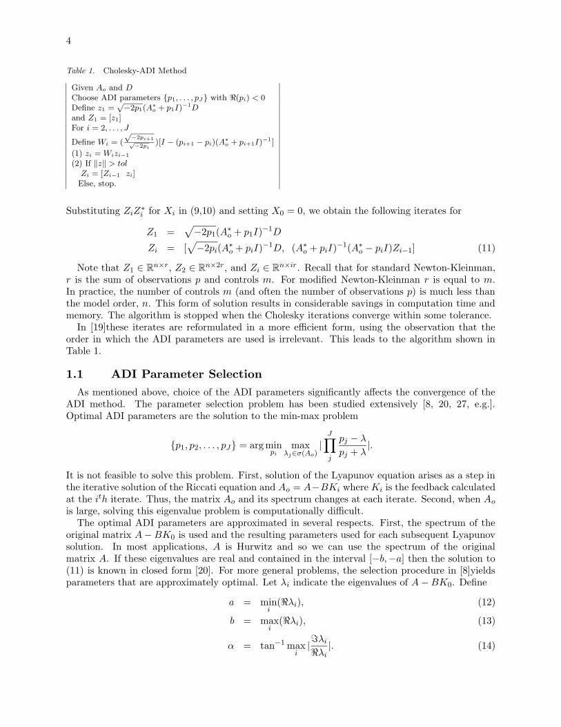
Table 1. Cholesky-ADI Method

Given Ao and DChoose ADI parameters {p1, . . . , pJ} with !(pi) < 0Define z1 =

"#2p1(A

!o + p1I)"1D

and Z1 = [z1]For i = 2, . . . , J

Define Wi = (""2pi+1#"2pi

)[I # (pi+1 # pi)(A!o + pi+1I)"1]

(1) zi = Wizi"1

(2) If $z$ > tolZi = [Zi"1 zi]Else, stop.

Substituting ZiZ"i for Xi in (9,10) and setting X0 = 0, we obtain the following iterates for

Z1 ="$2p1(A"o + p1I)#1D

Zi = ["$2pi(A"o + piI)#1D, (A"o + piI)#1(A"o $ piI)Zi#1] (11)

Note that Z1 # Rn%r, Z2 # Rn%2r, and Zi # Rn%ir. Recall that for standard Newton-Kleinman,r is the sum of observations p and controls m. For modified Newton-Kleinman r is equal to m.In practice, the number of controls m (and often the number of observations p) is much less thanthe model order, n. This form of solution results in considerable savings in computation time andmemory. The algorithm is stopped when the Cholesky iterations converge within some tolerance.

In [19]these iterates are reformulated in a more e"cient form, using the observation that theorder in which the ADI parameters are used is irrelevant. This leads to the algorithm shown inTable 1.

1.1 ADI Parameter SelectionAs mentioned above, choice of the ADI parameters significantly a!ects the convergence of the

ADI method. The parameter selection problem has been studied extensively [8, 20, 27, e.g.].Optimal ADI parameters are the solution to the min-max problem

{p1, p2, . . . , pJ} = argminpi

max!j'"(Ao)

|J#

j

pj $ "

pj + "|.

It is not feasible to solve this problem. First, solution of the Lyapunov equation arises as a step inthe iterative solution of the Riccati equation and Ao = A$BKi where Ki is the feedback calculatedat the ith iterate. Thus, the matrix Ao and its spectrum changes at each iterate. Second, when Ao

is large, solving this eigenvalue problem is computationally di"cult.The optimal ADI parameters are approximated in several respects. First, the spectrum of the

original matrix A$BK0 is used and the resulting parameters used for each subsequent Lyapunovsolution. In most applications, A is Hurwitz and so we can use the spectrum of the originalmatrix A. If these eigenvalues are real and contained in the interval [$b,$a] then the solution to(11) is known in closed form [20]. For more general problems, the selection procedure in [8]yieldsparameters that are approximately optimal. Let "i indicate the eigenvalues of A$BK0. Define

a = mini

(("i), (12)

b = maxi

(("i), (13)

# = tan#1 maxi

|)"i

("i|. (14)

Solution of Algebraic Riccati Equations Arising in Control of Partial Di!erential Equations 5

These parameters determine an elliptic domain # that contains the spectrum and is used to deter-mine the ADI parameters pi. The closeness of # to the smallest domain containing the spectruma!ects the number of iterations required for convergence of the Cholesky-ADI. The parameter # isthe maximum angle between the eigenvalues and the real axis. When the spectrum contains lightlydamped complex eigenvalues, # is close to $/2. In this case, # is a poor estimate of this domain.This point is investigated in the third example below.

2. Benchmark ExamplesIn this section we test the algorithm with a number of standard examples: a one-dimensional

heat equation, a two-dimensional partial di!erential equation and a beam equation. All computa-tions were done within MATLAB on a a computer with two 1.2 GHz AMD processors. (Shortercomputation time would be obtained by running optimized code outside of a package such as MAT-LAB. The CPU times are given only for comparision purposes.) The relative error for the Choleskyiterates was set to 10#8.

2.1 Heat EquationConsider the linear quadratic regulator problem of minimizing a cost functional [2, 7]

J(u) =! !

0(|Cz(t)|2 + |u(t)|2)dt

subject to

%z(t, x)%t

=%2z(t, x)

%x2, x # (0, 1),

z(0, x) = &(x) (15)

with boundary conditions

%z(t, 0)%x

= u(t)

%z(t, 1)%x

= 0. (16)

Setting

Cz(t) =! 1

0z(t, x)dx, (17)

and R = 1, the solution to the infinite-dimensional Riccati equation is

Kz =! 1

0k(x)z(x)dx

where k = 1 [3]. Thus, for this problem we have an exact solution to which we can compare theapproximations.

The equations (14-17) are discretized using the standard Galerkin approximation with linearspline finite element basis on an uniform partition of [0, 1]. The resulting A matrix is symmetricand tridiagonal while B is a column vector with only one non-zero entry. Denote each basis elementby li, i = 1..n. For an approximation with n elements, the approximating optimal feedback operatorK is

Kz =! 1

0kn(x)z(x)dx, (18)

6

Newton-Kleinmann Iteration Optimal Feedback Gain1 50.0052 25.01253 12.52624 6.3035 3.23086 1.77027 1.16758 1.0129 1.000110 111 1

Table 2. Heat Equation: Feedback Gain at each Newton-Kleinman Iteration

Table 3. Heat Equation: Standard Newton-Kleinman Iterations

n Newton-Kleinman Itn’s Lyapunov Itn’s CPU time25 11 19,22,23,26,27,29 0.83

30,31,31,31,3150 11 24,26,28,30,32,34 1.2

35,35,35,35,35100 11 28,31,32,35,36,38 3.49

39,40,40,40,40200 11 33,35,37,39,41,43 23.1

44,44,44,44,44

where kn(x) =$n

i=1 kili(x). The solutions to the approximating Riccati equations converge [3,13]and so do the feedback operators.

Table 2 shows the approximated optimal feedback gain at each Newton-Kleinman iteration. Thedata in Table 2 is identical for n = 25, 50, 100, 200 and for both Newton-Kleinman methods.The error in K versus Newton-Kleinman iteration in shown in Figure 1 for standard Newton-Kleinman and in Figure 2 for the modified algorithm. In Tables 3 and 4 we compare the numberof Newton-Kleinman and Lyapunov iterations as well as the CPU time per order n. We use theansatz k0(x) = 100 for all n. With the modified algorithm, there are 1$ 2 fewer Riccati loops thanwith the the original Newton-Kleinman iteration. Also, the modified Newton-Kleinman methodrequires fewer Lyapunov iterations within the last few Newton-Kleinman loops. The computationtime with the modified Newton-Kleinman algorithm is significantly less than that of the originalalgorithm.

2.2 Two-Dimensional ExampleDefine the rectangle # = [0, 1]% [0, 1] with boundary %#. Consider the two-dimensional partial

di!erential equation [7]

#z#t = #2z

#x2 + #2z#y2 + 20#z

#y + 100z = f(x, y)u(t), (x, y) # #z(x, y, t) = 0, (x, y) # %#

(19)

where z is a function of x, y and t. Let

f(x, y) =%

100, if .1 < x < .3 and .4 < y < .60, else .

Solution of Algebraic Riccati Equations Arising in Control of Partial Di!erential Equations 7

Table 4. Heat Equation: Modified Newton-Kleinman Iterations

n Newton-Kleinman Itn’s Lyapunov Itn’s CPU time25 10 19,22,23,26,27,29 0.66

30,31,29,150 10 24,26,28,30,32,34 0.94

35,35,33,1100 9 28,31,32,35,36,38 2.32

39,40,1200 9 33,35,37,39,41,43 14.2

44,44,1

Table 5. Iterations for 2-d Equation (Newton-Kleinman)

grid K0 n Newton-Kleinman Itn’s Lyapunov Itn’s CPU time12% 12 0 144 14 12,44,41,39,36,34,32 4.98

30,28,27,27,27,27,2723% 12 0 276 15 16,47,45,42,40,38,35,33 22.2

31,30,30,30,30,30,3023% 12 K12x12

proj 276 6 29,30,30,30,30,30 10.823% 23 0 529 16 20,51,48,46,44,41,39,37 139.

35,34,33,33,32,32,32,3223% 23 K23x12

proj 529 5 33,32,32,32,32 65.7

Central di!erence approximations are used to discretize (19) on a grid of N % M points. Theresulting approximation has dimension n = N %M : A # Rn%n and B # Rn%1. The A matrix issparse with at most 5 non-zero entries in any row. The B matrix is a sparse column vector. Wechose C = B" and R = 1.

We solved the Riccati equation on a number of grids, using both standard and modified Newton-Kleinman methods. The data is shown in Tables 5 and 6. Modified Newton-Kleinman is clearlymuch more e"cient. Fewer Lyapunov iterations are required for convergence and this leads to areduction in computation time of nearly 50%.

We also investigated the use of non-zero initial estimates for K in reducing computation time.We first solve the Riccati equation on a 12 % 12 grid. Since !(A) & C#, K144

0 = 0 is a possibleansatz. It required 13 Newton-Kleinman iterations and a total of 419 Lyapunov iterations to obtaina relative error in K of 10#11. Linear interpolation was used to project this solution to a functionon a finer grid, 23 % 12, where n = 276. Indicate this projection by K12%12

proj . On the finer grid23% 12 where n = 276, we used both zero and K12%12

proj as initial estimates. As indicated in Table 6,the error of K was 10#12 after only 150 Lyapunov and 54 Newton-Kleinman iterations. The sameprocedure is applied to generate a guess K529

0 where the mesh is 23% 23 and n = 529. Neglectingthe computation time to perform the projection, use of a previous solution lead a total computationtime over both grids of only 6.3 seconds versus 11.9 seconds for n = 276 and a total computationtime of only 27.8 versus 79.5 for n = 529. Similar improvements in computation time were obtainedwith standard Newton-Kleinman.

3. Euler-Bernoulli BeamConsider a Euler-Bernoulli beam clamped at one end (r = 0) and free to vibrate at the other

end (r = 1). Let w(r, t) denote the deflection of the beam from its rigid body motion at time t andposition r. The deflection is controlled by applying a a torque u(t) at the clamped end (r = 0).

8

Table 6. Iterations for 2-d Equation (Modified Newton-Kleinman)

grid K0 n Newton-Kleinman Itn’s Lyapunov Itn’s CPU time12% 12 0 144 13 12,44,41,39,36,34,32 2.94

30,28,27,27,27,123% 12 0 276 13 16,47,45,42,40,38,35 11.9

33,31,30,30,30,2923% 12 K12x12

proj 276 4 29,30,30,29 3.3623% 23 0 529 14 20,50,48,46,44,41,39 79.5

37,35,34,33,33,33,3123% 23 K23x12

proj 529 4 33,32,32,1 21.5

We assume that the hub inertia Ih is much larger than the beam inertia Ib so that Ih' * u(t). Thepartial di!erential equation model with Kelvin-Voigt and viscous damping is

wtt(r, t) + Cvwt(r, t) +%2

%r2

&CdIbwrrt(x, t) +

EIr

(Awrr(r, t)

'=

(r

Ihu(t), (20)

with boundary conditions

w(0, t) = 0wr(1, t) = 0.

EIwrr(1, t) + CdIbwrrt(1, t) = 0%

%r[EI(1)wrr(r, t) + CdIbwrrt(r, t)]r=1 = 0.

The values of the physical parameters in Table 1.3 are as in [1].Define H be the closed linear subspace of the Sobolev space H2(0, 1)

H =%

w # H2(0, 1) : w(0) =dw

dr(0) = 0

(

and define the state-space to be X = H%L2(0, 1) with state z(t) = (w(·, t), ##tw(·, t)). A state-space

formulation of the above partial di!erential equation problem is

d

dtx(t) = Ax(t) + Bu(t),

where

A =

)

*0 I

$EI$

d4

dr4 $CdI$

d4

dr4 $ Cv$

+

, , B =

)

*0

rIh

+

, ,

with domain

dom (A) = {(), &) # X : & # H and

M = EI d2

dr2 ) + CdId2

dr2 & # H2(0, 1) with M(L) = ddrM(L) = 0} .

We use R = 1 and define C by the tip position:

w(1, t) = C[w(x, t) w(x, t)].

Solution of Algebraic Riccati Equations Arising in Control of Partial Di!erential Equations 9

E 2.68% 1010 N/m2

Ib 1.64% 10"9 m4

! 1.02087 kg/mCv 1.8039 Ns/mCd 1.99% 105 Ns/mL 1 mIh 121.9748 kg m2

d .041 kg"1

Table 7. Table of physical parameters.

Let HN & H be a sequence of finite-dimensional subspaces spanned by the standard cubic B-splines with a uniform partition of [0, 1] into N subintervals. This yields an approximation inHN %HN [14, e.g.]of dimension n = 2N.

This approximation method yields a sequence of solutions to the algebraic Riccati equation thatconverge strongly to the solution to the infinite-dimensonal Riccati equation corresponding to theoriginal partial di!erential equation description [3, 21].

The spectrum of A for various n is shown in Figure 4. For small values of n, the spectrum ofAn only contains complex eigenvalues with fairly constant angle. As n increases, the spectrumcurves into the real axis. For large values of n, the spectrum shows behaviour like that of theoriginal di!erential operator, and contains two branches on the real axis. For these large values ofn, the ADI parameters are complex numbers. We calculated the complex ADI parameters as in[8]. Although there are methods to e"ciently calculate with complex parameters by splitting thecalculation into 2 real parts [19]their presence increases computation time.

Figure 5 shows the total Lyapunov iterations for various values of n. Although the number ofNewton-Kleinman iteration remained at 2 for all n, the number of Lyapunov iterates increases asn +,.

Figure 6 shows the change in the spectrum of A as Cd is varied. Essentially, increasing Cd

increases the angle that the spectrum makes with the imaginary axis. Recall that the spectralbounds #, a, and b define the elliptic function domain that contains the spectrum of A [20]. TheADI parameters depend entirely on these bounds. The quantity %

2 $ # is the angle between thespectrum and the imaginary axis and so # + $/2 as Cd is decreased. Figure 7 shows the e!ect ofvarying Cd on the number of iterations required for convergence. Larger values of Cd (i.e. smallervalues of #) leads to a decreasing number of iterations. Small values of Cd lead to a large numberof required iterations in each solution of a Lyapunov equation.

There are several possible reasons for this. As the spectrum of A flattens with increasing Cd

the spectral bounds (12-14) give sharper estimates for the elliptic function domain # and thus theADI parameters are closer to optimal. Improvement in calculation of ADI parameters for problemswhere the spectrum is nearly vertical in the complex plane is an open problem.

Another explanation lies in the nature of the mathematical problem being solved. If Cd > 0the semigroup for the original partial di!erential equation is parabolic and the solution to theRiccati equation converges uniformly in operator norm [16, chap.4]. However, if Cd = 0, the partialdi!erential equation is hyperbolic and only strong convergence of the solution is obtained [17].Thus, one might expect a greater number of iterations in the Lyapunov loop to be required as Cd isdecreased. Any X # Rn%n to the matrix Lyapunov equation is symmetric and positive semi-definiteand so we can order its eigenvalues "1 - "2 - ..."n - 0. The ability to approximate X by a matrixof lower rank X is determined by the following relation [11, Thm. 2.5.2]

minrankX(k#1

.X $ X..X. =

"k(X)"1(X)

.

10

Table 8. Beam: : E!ect of Changing Cd (Standard Newton-Kleinman)

Cv Cd " Newton-Kleinman Itn’s Lyapunov Itn’s CPU time2 1% 104 1.5699 – – –

3% 105 1.5661 – – –4% 105 1.5654 3 1620;1620;1620 63.141% 107 1.5370 3 1316;1316;1316 42.911% 108 1.4852 3 744;744;744 18.015% 108 1.3102 3 301;301;301 5.32

Table 9. Beam: E!ect of Changing Cd (Modified Newton-Kleinman)

Cv Cd " Newton-Kleinman It’s Lyapunov It’s CPU time2 1% 104 1.5699 2 – –

3% 105 1.5661 2 – –4% 105 1.5654 2 1620;1 24.831% 107 1.5370 2 1316;1 16.791% 108 1.4852 2 744;1 7.495% 108 1.3102 2 301;1 2.32

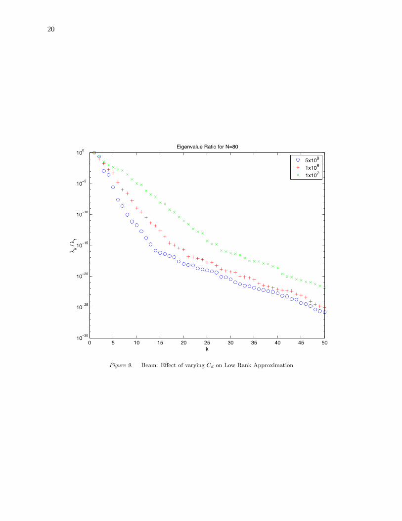
This ratio is plotted for several values of Cd in Figures 8 and 9. For larger values of Cd the solutionX is closer to a low rank matrix than it is for smaller values of Cd. Recall that the CF-ADIalgorithm used here starts with a rank 1 initial estimate of the Cholesky factor and the rank ofthe solution is increased at each step. The fact that the solution X is closer to a low rank matrixfor larger values of Cd implies a smaller number of iterations are required for convergence. If thefundamental reason for the slow convergence with small Cd is the “hyperbolic-like” behaviour ofthe problem, then this convergence will not be improved by better ADI parameter selection. Thismay have consequences for control of coupled acoustic-structure problems where the spectra arecloser to those of hyperbolic systems than those of parabolic systems.

References

[1] H.T. Banks and D. J. Inman, “On Damping Mechanisms in Beams”, ICASE Report No. 89-64, NASA, Langley,1989.

[2] H. T. Banks and K. Ito, A Numerical Algorithm for Optimal Feedback Gains in High Dimensional LinearQuadratic Regulator Problems, SIAM J. Control Optim., vol. 29, no. 3, 499-515, 1991.

[3] H. T. Banks and K. Kunisch, The linear regulator problem for parabolic systems, SIAM J. Control Optim., vol.22, 5, 684-698, 1984.

[4] R.H. Bartels and W. Stewart, “Solution of the matrix equation AX+XB =C” Comm. of ACM, Vol. 15, pg.820-826, 1972.

[5] D. Bau, and L. Trefethen, Numerical Linear Algebra, SIAM, Philadephia, 1997.

[6] J.A. Burns and K. P. Hulsing, “Numerical Methods for Approximating Functional Gains in LQR BoundaryControl Problems”, Mathematical and Computer Modelling, vol. 33, no. 1, pg. 89-100, 2001.

[7] Y. Chahlaoui and P. Van Dooren, A collection of Benchmark examples for model reduction of linear timeinvariant dynamical systems, SLICOT Working Note 2002-2, http://www.win.tue.nl/niconet/

[8] N. Ellner and E. L. Wachpress, Alternating Direction Implicit Iteration for Systems with Complex Spectra, SIAMJ. Numer. Anal., vol. 28, no. 3, 859-870, 1991.

[9] J.S. Gibson, “The Riccati Integral Equations for Optimal Control Problems on Hilbert Spaces”, SIAM J. Controland Optim., Vol. 17, pg. 637-565, 1979.

[10] J.S. Gibson, “Linear-quadratic optimal control of hereditary di!erential systems: infinite dimensional Riccatiequations and numerical approximations”, SIAM J. Control and Optim., Vol. 21 95-139, 1983.

[11] G.H. Golub and C.F. van Loan, Matrix Computations, John Hopkins, 1989.

[12] J.R. Grad and K. A. Morris, “Solving the Linear Quadratic Control Problem for Infinite-Dimensional Systems”,Computers and Mathematics with Applications, Vol. 32, No. 9, 1996, pg. 99-119.

[13] K. Ito, Strong convergence and convergence rates of approximating solutions for algebraic Riccati equations inHilbert spaces, Distributed Parameter Systems, eds. F. Kappel, K. Kunisch, W. Schappacher, Springer-Verlag,1987, 151-166.

[14] K. Ito and K. A. Morris, An approximation theory of solutions to operator Riccati equations for H$ control,SIAM J. Control Optim., 36, 82-99, 1998.

[15] D. Kleinman, On an Iterative Technique for Riccati Equation Computations, IEEE Transactions on Automat.Control, 13, 114-115, 1968.

[16] I. Lasiecka and R. Triggiani, Control Theory for Partial Di!erential Equations: Continuous and ApproximationTheories, Part 1, Cambridge University Press, 2000.

[17] I. Lasiecka and R. Triggiani, Control Theory for Partial Di!erential Equations: Continuous and ApproximationTheories, Part 2, Cambridge University Press, 2000.

[18] A.J. Laub, “A Schur method for solving algebraic Riccati equations”, IEEE Trans. Auto. Control, Vol. 24, pg.913-921, 1979.

12

[19] J. R. Li and J White, Low rank solution of Lyapunov equations, SIAM J. Matrix Anal. Appl., Vol. 24, pg.260-280, 2002.

[20] A. Lu and E. L. Wachpress, Solution of Lyapunov Equations by Alternating Direction Implicit Iteration, Com-puters Math. Applic., 21, 9, 43-58, 1991.

[21] K.A. Morris, “Design of Finite-Dimensional Controllers for Infinite-Dimensional Systems by Approximation”,J. Mathematical Systems, Estimation and Control, 4, 1-30, 1994.

[22] K.A. Morris, Introduction to Feedback Control, Harcourt-Brace, 2001.

[23] T. Penzl, “A Cyclic Low-Rank Smith Method for Large Sparse Lyapunov Equations”, SIAM J. Sci. Comput.,Vol. 21, No. 4, pg. 1401-1418, 2000.

[24] I. G. Rosen and C. Wang, “A multilevel technique for the approximate solution of operator Lyapunov andalgebraic Riccati equations”, SIAM J. Numer. Anal. Vol. 32 514–541, 1994.

[25] Russell, D.L., Mathematics of Finite Dimensional Control Systems: Theory and Design, Marcel Dekker, NewYork, 1979.

[26] R.A. Smith, “Matrix Equation XA + BX = C”, SIAM Jour. of Applied Math., Vol. 16, pg. 198-201, 1968.

[27] E. L. Wachpress, The ADI Model Problem, preprint, 1995.

[28] E. Wachpress, “Iterative Solution of the Lyapunov Matrix Equation”, Appl. Math. Lett., Vol. 1, Pg. 87-90, 1988.

REFERENCES 13

1 2 3 4 5 6 7 8 9 10 1110−9

10−8

10−7

10−6

10−5

10−4

10−3

10−2

10−1

100

Error

Iterations

N=25N=50N=100N=200

Figure 1. Heat Equation: Error versus Standard Newton-Kleinman Iterations

1 2 3 4 5 6 7 8 9 1010−14

10−12

10−10

10−8

10−6

10−4

10−2

100

Error

Iterations

N=25N=50N=100N=200

Figure 2. Heat Equation: Error versus Modified Newton-Kleinman Iterations

14

0 2 4 6 8 10 12 1410−14

10−12

10−10

10−8

10−6

10−4

10−2

100

Error

Iterations

N=144N=276N=529

Figure 3. Convergence rate for two-d problem (modified Newton-Kleinman). Initial estimates: K144 = 0, K276 =K144

proj , K529 = K276proj

REFERENCES 15

−6 −5 −4 −3 −2 −1 0x 105

−4−2

024

x 104

−6 −5 −4 −3 −2 −1 0x 105

−4−2

024

x 104

−6 −5 −4 −3 −2 −1 0x 105

−4−2

024

x 104

−6 −5 −4 −3 −2 −1 0x 105

−4−2

024

x 104

Figure 4. Beam: spectrum of An for n = 48, 56, 64, 88 (Cd = 9% 105).

16

45 50 55 60 65 70 75 80 85 901000

1500

2000

2500

3000

3500

4000

4500

5000

n

Lyap

unov

Iter

atio

ns

Figure 5. Beam: n vs. Lyapunov Iterations (Cd = 9% 105)

REFERENCES 17

−5 −4.5 −4 −3.5 −3 −2.5 −2 −1.5 −1 −0.5 0x 104

−5

0

5

x 104

−5 −4.5 −4 −3.5 −3 −2.5 −2 −1.5 −1 −0.5 0x 104

−5

0

5

x 104

−5 −4.5 −4 −3.5 −3 −2.5 −2 −1.5 −1 −0.5 0x 104

−5

0

5

x 104

Figure 6. Beam: Spectrum of A for Cd = 1x104, 4x105, 1x108 (n = 80)

18

0 0.5 1 1.5 2 2.5 3 3.5 4 4.5 5x 108

500

1000

1500

2000

2500

3000

3500

Cd

Lyap

unov

Iter

atio

ns

1.48 1.5 1.52 1.54 1.56 1.580

2

4

6

8

10x 107

α

C d

Figure 7. Beam: E!ect of Cd on Lyapunov Iterations and " (n = 80)

REFERENCES 19

0 5 10 15 20 25 30 35 40 45 5010−30

10−25

10−20

10−15

10−10

10−5

100

k

λ k / λ 1

Eigenvalue Ratio for N=64

5x108

1x108

1x107

Figure 8. Beam: E!ect of varying Cd on Low Rank Approximation

20

0 5 10 15 20 25 30 35 40 45 5010−30

10−25

10−20

10−15

10−10

10−5

100

k

λ k / λ 1

Eigenvalue Ratio for N=80

5x108

1x108

1x107

Figure 9. Beam: E!ect of varying Cd on Low Rank Approximation