Embed Size (px)
Citation preview

S-NET THEORY AND MODELING OF SYSTEM
K S SIVANANDAN
ELECTRICAL ENGINEERING DEPARTMENT NATIONAL INSTITUTE OF TECHNOLOGY
CALICUT.
KERALA - INDIA – 673 601

CHAPTER 1
INTRODUCTION
S-Net theory is a tool for the study of system. This theory allows a system to be
modeled by an S-Net. Analysis of the S-Net can the hope fully, revel important
information about the performance of the system. This information can be used to
evaluate the modeled system and suggest improvements or changes. Thus, the
development of a theory of S-Net is based on the application of S-Net in the modeling,
analysis and design of system.
The application of S-Nets is through modeling. In many fields of study, a
phenomenon is not studied directly but indirectly through a model of the phenomenon. A
model s a representation, often in mathematical terms of what are felt to be the important
features of the object or system under study. By the manipulation, it is hoped that new
knowledge about the modeled phenomenon can be obtained with out the danger, cost or
inconvenience of manipulating the real phenomenon itself. Intuitive graphical
representation and the powerful algebraic formulations of S nets have lead to their use in
a number of fields. S nets are used to model computer communication systems,
manufacturing assembly line, flexible manufacturing systems, strategic application
systems, instrumentation systems, process control systems, physiological control systems
etc. Often times the graphical representation of a plant, as an S net model is enough for
the plant. Through the study of structural variance and invariance of S net, which
are actually elements of the Kernel of the S net incidence matrix, and an application of
some of the elementary concepts, possibilities can be explored for S net-based plant
models, for effective performance evaluation. Examples of the use of modeling include
astronomy (Where models of the birth, death and interaction of stars allow studying
theories which would take long times and massive amounts of matter and energy),
2

nuclear physics (Where the radioactive atomic and sub- atomic particles under study
exists for very short periods of time.), sociology, (Where the direct manipulation of
groups of people for study might cause ethical problems), Biology (Where models of
biological systems require less space, time and food to develop), and so on.
Most modeling uses mathematics. The important features of many physical
phenomenons can be described numerically and the relations between these features
described by equations or inequalities. Particularly in the natural sciences and
engineering, properties such as mass, position, momentum, acceleration and forces are
describable by mathematical equations. To successfully utilize the modeling approach,
however requires knowledge of both the modeled phenomena and the properties of the
modeling techniques. Thus mathematics has developed as a science in part because of its
usefulness in modeling the phenomena of other sciences. For example, differential
calculus was developed in direct response to the need for a means of modeling
continuously changing properties such as position, velocity, and accelerations in physics.
The developments of high-speed computers have greatly increased the use and
usefulness of modeling. By representing a system as a mathematical model, converting
that model into instructions for a computer, and running the computer, it is possible to
model larger and more complex systems than over before This has restricted in
considerable study of computer modeling techniques and of computers themselves.
Computers are involved in modeling in to ways: as a computational tool for modeling and
as a subject of modeling.
Computer system is very complex, often large, system of many interacting
components. Such component can be quiet complex, as can its interaction with other
components in the system. This is also true of many other systems. Economic systems,
legal systems traffic control systems, chemical systems and physiological systems all
involve many individual components interacting with other components, possibly in
complex ways. Thus, despite the diversity of systems that want to model, several
common points stand out. These should then be features of a useful model of these
systems. One fundamental idea is that systems are composed of separate, interacting
3

components. Such component may itself be a system, but its behavior can be described
independently of other components of the systems, except for well-defined interactions
with other components. Each component has its own state of being. The state of a
component is an abstraction of the relevant information necessary to describe its (future)
actions. Often the state of component depends on the past history of the component.
Thus the state of a component may change over time. The concept of “state” is very
important to modeling a component . For example, in queuing system model of blank,
there may be several consumes. Tellers may be either idle (waiting for a customer to
need service) or busy (bring served by a letter). Similarly, the customers may be idle
(waiting for a teller to be free to serve them) or busy (being served by a teller). In a
model of a hospital, the state of a patient might be critical, serious, fair, good or excellent.
The components of a system exhibit concurrency or parallelism. Activities of the
component of a system may simultaneously with other activities of other components.. in
a computer systems, for example peripheral devices, such as floppy drives, printers and
so on may all operate concurrently under the control of the computer in an economic
system manufactures may be producing some products while retailers are selling other
products and consumers are using still other products all at the same time.
The concurrent nature of activity in a system creates some difficult modeling
problems. Since the components of the systems interact, it is necessary for
synchronization to occur. The transfers of information or materials from one component
to another require that the activities of the involved component be synchronized while the
interaction is occurring. This may result ion one component waiting for another
component. The timing of action of different components may be very complex and the
resulting interaction between components difficult to describe.
History of S-Nets.
S-Net theory is developed to model the above-mentioned types of systems. The
theory has been developed from the early work of the author (1987). In his doctoral
desertion “on the enhancement of timed pertinent theory and its applications to some
aspects of computer systems”, the author formulated the basis for a theory for the
4

modeling and analysis of computer systems in early 1980’s. The desertion was mainly a
theoretic development of the basic concepts of S-Net theory named as APN (Advanced
Pertinent theory) as mentioned in the desertion. Basic concept of the theory appeared in
the proceedings of the second d International conference” On supercomputing “SANTA
CLARA, CA USA May 3-2 1987.another application of the theory appeared by taking a
head line as ON THE PETRINET MODELING OF MEDIIUM ACCESS PROTOCOLS”
in the proceedings of IEEE TENCON 90 - IEEE region to conference on computer and
communications systems in 1990. the application of APN theory to take resource sharing
problems suggested through an articles ON THE MODELING AND ANALYSIS OF
RESOURCE SHARING PROBLEMS BY AN ADVANCED PETRINET” in the
proceedings of the “International conference modeling and simulation” NEW
ORLEANS, LOUISIANA (USA) – OCTOBER 28-3-1992.
The application of APN ’s also cited in some project report of Regional
Engineering Collage Calicut library, which were submitted as the partial fulfillment of
some undergraduates and post graduate degree of University of Calicut during 1990-
2001.periods.
Subsequently the author was continuously working on the above theory to
improve the theory for better utility in the field of applied science and technology during
this process the postulator extended its utility to software development and virtual reality
applications and renamed as S-Net theory in 1992. Prof. Narahari of school of
automation of the Indian Institute of Science, Bangalore sole hearted by provided the
moral courage and necessary scientific advice for the venture.
Application of S-Net theory in the software development area is described in the
paper “S-Net theory - A foundation for the developed of software packages for distinct
objectives in the proceedings of the CAD/CAM conference-Regional Engineering
Collage, Calicut 1992 - Kerala, India. (Ref. No. ).
The performance evaluation and suggestion for improvement of instrumentation
system and strategic system can be done effectively by using S-Net theory. Postgraduate
5

dissertation report of Mr. Narasimha Rao and Mr. Aruna of Regional Engineering
Collage Calicut, Kerala, India in the year 1998-1999 and 1999-2000 lights this matter.
APPLYING S-NET THEORY
Design, analysis and evaluation of modern systems can be accomplished in
several ways. Physical, structural, architectural and operational characteristics are
studied first in a conceptual and qualitative way. It helps for the development of S-Net
models of the system. S-Net model is then analyzed. Analysis helps the evaluator to
suggest necessary alterations in the structural, physical, architectural and operational
characteristics of the modeled system. Modified system is again subjected to modeling,
analysis and there by getting the cycle repeated until analysis reveals no unacceptable
problems. This approach is diagramed in Fig.1.1. Note that this approach can also be
used to analyze an existing, currently operational system.
Qualitative Study Revise Analysis
SYSTEM
Analytical properties of the System through Results
Physical, Architectural and Operational Characteristics
of the system
S-Net Models
6

CHAPTER II
DEVELOPMENT OF S NET THEORY
INTRODUCTION
S-net theory as a member of Petrinet family came into being during 1980’s
and1990’s. Basic Petrinet formalism is extended in a variety of way’s and as result many
members came into the family of Petrinet. These members helped either to impart more
modeling power or to enable domain specific features to be modeled more conveniently
and easily[1,2, ]. The author postulated the early version of S-NET THEORY in the
middle of 1990’s [1,2 ].The motivation behind the work is to provide a much more easy
and convenient modeling tool. S-NET models, the author believes, have an appealing
graphical representation. It is possible to visualize the state of flow of a system and to
quickly see dependencies of one part of a system on another when the system is
represented as an S – NET.
Here a formal qualitative description about the basic concepts of S NETs is
presented. These basic concepts are used through this work on S – NET and so are
fundamental to a correct understanding of S- NET.
Formalism adopted here are based on bag theory, an extension of set theory. If
unfamiliar ties exits with bag theory, it is suggested to read the appendix for the relevant
concepts.
The definitions given here bears good familiarity in style to definitions in
automata theory [Hopcroft and Ulman 1969].
7

As in the case of Petrinet, S- NET is made up of places, which holds tokens,
transitions and directed arcs between the places and transitions. The number and
distributions of tokens among the places is called the marking and represents the state of
the net. The arcs determine how tokens move from one place to another upon the firing of
a transition .The state of a system can be represented as an integer vector, the architecture
or lay out of an S NET can be represented with an integer matrix known as the incidence
matrix. Having mentioned this a detailed description about the formulation of the S NET
is discussed as under for better understanding.
2.1 OVERVIEW OF S NET
The S net (S NET) is an enhancement of the ordinary Petrinet. It facilitates
ease of representation of some specific complex features of systems such as, Flexible
manufacturing systems, Supercomputer architectures, Computer communication systems
and networks, computer controlled data acquisition systems, Process control Systems etc.
The proposal of new basic fundamental concepts and development of efficient
analysis techniques obtain simplicity and convenience of representation in modeling and
analysis. The proposed new basic fundamental concepts are classified as follows:
a. New basic fundamental concepts in the category of places
b. New basic fundamental concepts in the category of tokens
8

c. New basic fundamental concepts in the category of transitions
d. New basic fundamental concepts in the category of arcs
e. New basic fundamental concepts in the category of transitions
These new basic fundamental concepts are discussed below.
New Basic fundamental concepts for Places
Under this category the main concepts are
a New type of places called source places
b New type of places called sink places
c Attachment of identity /colour to places as well as tokens.
These main primitive concepts create some associated primitive concepts, described
as follows:
Source places are associated with the concepts of
i) Arrival of tokens from external world in to the net.
ii) Token arrival time.
iii) Generation time and Generation interval of token.
Sink places are associated with the concept of dead tokens.
As a combined effect of source and sink places, a new concept called lifetime is also
put in.
Attachment of identity of places automatically resulted the concept of the
attachment of identity to tokens as well as to arcs. This lead to the transfer of tokens ( by
the firing of transitions ), to be governed by certain identity regulations through the newly
developed firing rules. Stay of tokens in places is also governed by the identity.
9

New Basic fundamental concepts for Transitions
These new primitive concepts are described as follows:
Single coloured input, Multicoloured output (SIMO), Multicoloured input,
Multicoloured output (MIMO), Sink Related Transitions (SRT). Associated with this
main fundamental concept, there are some associated concepts, such as:
a) Attachment of special firing rules
b) Generation of new tokens with new identity inside the net by the firing of these
transitions
c) Repeatability number
New Basic fundamental concepts for Arcs
In the case of arcs, a new concept of assigning weights has been proposed so that
a) Weights are realized as function of time,
b) Weights are also realized as functions of the magnitude of tokens at the input/output
places.
Apart from this, arcs also have identity. This identity of arcs regulates the
movement of tokens. Transitions are also characterized on the basis of the identity
attached with their input/output arcs.
In order to have a complete understanding of these concepts, detailed
explanations, definitions & examples are presented below.
10

2.2 COMPONENTS OF S NET
The main components of the S NET are places, transitions, input/output arcs and
tokens as in the case of conventional Petrinets. But the newly added primitive concepts to
the conventional components bring about a considerable change in their characteristics.
These are explained in detail as follows:
2.2.1 Places and Tokens
In an S NET, there are three types of places. Apart from the ordinary place of the
conventional Petrinet, there are two special types of places. These are
- Source places, and
- Sink places
Each place is associated with an identity (colour). A place can only hold tokens of the
same identity. In other words, an S NET token has identity attached to it. Apart from this,
there are two types of tokens in an S NET.
a) Tokens capable of enabling the transitions, as in the case of conventional nets
b) Tokens which cannot enable any transitions, i.e. tokens which are considered dead
(dead tokens).
Representation: -
In an S NET a place is represented in general as Pijk where
i indicates an index of the place in the net
j indicates its type (s for source, z for sink, o for ordinary)
k indicates its identity
11

2.2.1(a) Source place
Definition 3.1
A source place is defined as a place through which tokens are generated or
brought from the external world and acts only as an input place to some transition(s) but
not as an output place. Source places have the following properties:
(i) Generation of tokens or (entry of tokens from external world) is possible in any of the
following ways:
One at a time, one at regular intervals of time, in batches, batches of tokens at
regular interval of time, as a continuous function of time, as a discrete function of time,
random function of time, periodic functions of time, etc.
(ii) The time interval between consecutive arrivals may be the same or different.
Basically, the characteristics of the generation of a token at the source place is a property
of the modeled system.
(iii) Source places, as well as tokens are associated with an identity (colour) usually
represented by alphabets.
(iv) The possibility of presence of more than one source place in the same S NET
model is quite natural. Hence co-ordination of the timings of token
generations in co-course places is inevitable. To facilitate this some new basic
fundamental concepts are suggested. These are
- Initial time
- Generation time or generation interval and
- Time of generation with reference to initial time
12

In the time based analysis of S NET the above timing aspects have a lot of
significance. Each of these is explained below:
2.2.1 (a1) Initial time
In an S NET, the entry time of the first token(s) is considered as a reference time
for analysis. Generally this would be the starting time for a series of transitions to enable
and fire. Hence it is simply termed as initial time and is defined as under:
Definition 3.1.1
Initial time is defined as that time at which the token(s) first get generated in a
Source place and is taken as the reference time for all time based analysis.
2.2.1(a2) Generation time or generation interval
As mentioned above, source places are places through which tokens are generated
Or brought from the external world . If tokens are repeatedly generated , the time
interval between two consecutive generations is termed as generation time or generation
interval and is defined as follows:
Definition 3.1.2
Generation time or generation interval is defined as time interval between two
consecutive generations of tokens (S) in a source place. Its magnitude may be either, a
constant, variable or a changing function of time and is a property of the modeled system.
2.2.1(a3) Time of generation with reference to initial time
Repeated generation or arrival of tokens is possible in a source place. If the first
token comes at time ti, defined as initial time, (Definition 3.1.1), and the second, third,
fourth etc. Tokens arrive at times t1, t2, t3, t4 … then the time duration (t1 - ti), (t2 - t1), (t3 -
t2) ... i.e., the time duration between the consecutive arrivals is defined as generation
13

interval. (Definition 3.1.2). But the time intervals (t1 - ti), (t2 - ti), (t3 - ti) … etc. i.e., the
time duration between the respective instant of arrival and the initial time is termed as
time of generation with reference to initial time.
Definition 3.1.3
Time of generation with reference to initial time is defined as the time duration
between a token’s generation instant and the initial time.
2.2.1(a.4) Representation of source place
In general a source place in an S NET is represented as Pisk where
i indicates the index to the place, i.e. its number
s indicates the type, i.e. source
k indicates its identity
2.2.1(b) Sink place
Definition 3.2
A sink place is defined as one, which collects dead tokens. Sink places have the
following properties.
i) They can act only as output places to some transition and not as
input places.
ii) The tokens arriving at the sink places are said to be dead, i.e,they
cannot enable further transitions.
In an S NET, source places are associated with generation of tokens, whereas sink
places are associated with the death of tokens. This is the state of a token where it is no
longer useful for enabling any further transition. The concept of a dead token gives rise to
the concept of lifetime of each token. This is defined below.
14

Definition 3.3
Token lifetime
Token life time is defined as the time duration between the birth or generation of
a token at a source place or any output place of a special type of transition and its death at
a sink place.
2.2.1 (b1) Representation of Sink place
In general a sink place in an S NET is represented as Pizk where
i indicates the index to the place, i.e. its number
z indicates the type, i.e. sink
k indicates its identity (colour)
2.2.2 Input / Output arcs
Input (output) arcs of an S NET are associated with identity (colour). The identity
(colour) of an input (output) arc of a transition is decided by the identity (colour) of the
associated input (output) place. But there is an exception in the case of an SRT, where the
identity of both; input and output arcs of an SRT is the same as the identity (colour) of
the output place of SRT. This will be discussed in detail while discussing Transitions.
Taking these identity concepts as a common factor, there are two types of arcs in an
S NET. These are
- Constant weighted arcs as in Ordinary Petrinets.
- Variable weighted arcs.
Apart from this associated identity (colour), the constant weighted arcs of an S NET are
Similar to those of Ordinary Petrinets.
15

Assigning variable weights to arcs is a primitive concept introduced for the
S NET.
There are two types of variable weighted arcs. These are
a) Weights of the arc are a function of time or an independent variable.
b) Weights of the arc are a function of the number of tokens at the input
Place.
S NET arcs having variable weights are considered in more detail in subsequent
Section 2.2.4. for simplicity this concept is represented by arc weight function (AWP)
shortly.
2.2.3 Transitions
S NET transitions are mainly classified on the basis of the input-output places and
arcs associated with them. The type of operation, which the transition represents, is also
taken into consideration. The S NET consists of three special types of transitions, in
addition to the conventional transitions. The operation of the conventional transition is
exactly the same as in Ordinary Petrinets. The special types of transitions in the S NET
are:
1) Single coloured Input, Multicoloured Output (SIMO) transitions.
2) Multicoloured Input, Multicoloured Output (MIMO) transitions
3) Sink related transitions (SRT)
These transitions may or may not have variable - weighted input (output) arcs.
Special firing rules are associated with the above transitions. Unwieldy predicates, whose
parameters are tokens as in (Petrinets and NPNs), are eliminated so as to provide simple
16

analytical techniques for the above transitions. Each of these transitions is explained in
detail below. Just as source places are associated with the generation of tokens, so the
firing of these special type of transitions are also associated with generation of tokens
with an entirely new identity inside the net, i.e. the firing of these transitions creates new
tokens with new identity at their output places. The identity of a newly generated token is
decided by the identity of the respective output places at which it is getting generated.
The exact firing details are governed by special firing rules.
17

Fig 2.1 A TYPICAL S-NET
T3SRTP4OB
P6ZB
P5OC
P3ZA
P1SAP20A
T1SIMO T2MIMO
T40RD
18

2.2.3 (a) Single colour input, multicolour output (SIMO) transitions.
Definition 3.4
A SIMO transition is defined as one, which is connected to a single input arc of
the same colour, and multiple output arcs of different colours.
A simple example, which illustrates the use of the SIMO transition, is a translator
program (assembler or compiler) in a computer system where the source program is fed
to the assembler Pass 1 or equivalent compiler phase. Fig. 2.2 (a & b) shows a SIMO
transition representing the action of the translator. P1SR is the source place where the
token corresponding to the source program is generated. The source program is indicated
by a red token in place P1SR . The output of Pass 1 is different and is indicated by a blue
token at place P3OB. A copy of the source program required in pass 2 and which is also an
output of the translator is indicated as a red token at place P2OR.
It needs to be noted that a blue token is generated which is not present at the input
place of the SIMO transition (TSIMO). It has been generated purely by the firing of the
transition TSIMO. Such generation of new coloured tokens has already been explained in
Section 3.1.
A SIMO transition represents and illustrates the distinction between the different
types of inputs and outputs, unlike in Petrinets, where all types are indicated merely by
thepresence of identical tokens. Therefore, this kind of token identification/generation
helps in understanding and analyzing the net easily and conveniently. At the same time, it
maintains simplicity of analytical techniques due to the absence of functional
dependencies.
19

P30B
P20RCOPY OF
SOURCE PROGRAM
OUT PUT OF PASS 1 T(SIMO)
P1SR
SOURCE
TRANSLATER PHASE
OR PASS
FIG 2.2(a) -A SIMO TRANSITION (BEFORE FIRING)
P30B
T(SIMO)
P1SR
OUTPUT OF PASS 1 P20R
COPY OF SOURCE PROGRAM
TRANSLATER PHASE
OR PASS
SOURCE
FIG 2.2(b) -A SIMO TRANSITION (AFTER FIRING)
20
Another interpretation that can be given to Fig. 2.2 is that it represents the operation of a
computer-based controller in real time systems. Here the controller regulates the
movement of some devices and interacts with sensors and actuators. The system consists
of the input as the control program and the result of its execution is the signal that
appears as electrical pulses in the output part of the system. In this case, P1SR is the input
place where Input Control Program is fed before execution and is indicated by the red
token. P2OR is the output place to represent the storage of the program after execution.
TSIMO represents the execution of the program. P3OB is the output place where the blue
token represents the result of execution or the actuating signal generated by the execution
of the control program.
Further examples to illustrate the use of TSIMO Transition are considered in more
detail in section 3.5 at the end of this chapter.
2.2.3 (b) Multicolour input, multicolour output (MIMO) Transition
Definition 3.5
A MIMO transition is defined as one which is connected to input arcs as well as
Output arcs of different colours.
A MIMO transition can be used for modeling, for example, real-time multi-
tasking systems, which involve task synchronization. An important kind of task
synchronization found in real time system is cross stimulation. Cross stimulation occurs
when one task is waiting for a signal from another task before it can proceed further, for
example, in the classical producer - consumer system. Fig. 2.3 (a & b) shows the Petrinet
model of such a system, using a MIMO transition. In this figure, P1OR and P2OB represent
21

the tasks 1 and 2.A red token in P1OR represents the arrival of the signal from task 1 after
execution. A blue
22

P2OB
P1O
R
TASK NO 2
TASK NO 1
P3OR
SYNCHRONIZATION
TMIMOMO
FIG 2.3(a) -A MIMO TRANSITION (BEFORE FIRING)
P4OB
FIG 3.3(b) -A MIMO TRANSITION (AFTER FIRING)
P4OB
TASK NO 2
TASK NO 1
P3OR
SYNCHRONIZATION
P2OB
P1OR
TMIM
O
23

SENSOR
MOVING MECHANISM COMPUTE
R
REMOVING & PACKING
MECHANISM
FIG.2.4 (a)-LINE DIAGRAM OF A COMPUTER CONTROLLED PRODUCTION LINE
Token in P2OB represents the waiting state of task 2. The MIMO transition represents the
Synchronization of the two tasks. The output of TMIMO is the place P4OB, representing task
T5ORD
FIG. 2.4(b)- S-NET MODEL OF THE ABOVE SYSTEM
P1SA T1ORD P2OA T2SIMO P3 0A T3MIMO
4 4 P4ZA
P7ZC
P6OC
P8ZB
P5OBT4SRT
24

2 in its (continuing) state of execution and the place P3OR, representing the suspended
Task 1.
Another example to illustrate a MIMO transition is the packing system of a
computer-controlled production line (also called a Flexible Manufacturing System in
recent parlance) as shown in Fig. 2.4. Here the system packs X objects in one packet. A
computer counts the number of objects and when the number reaches X, it gives a signal
to move the object to a packet. The interpretation of various places is as under. Tokens in
P3OA represent the objects appearing at the packing site in the production line. P6OC
represents the place where the signal from the computer arrives. A colour C token in
place P6OC is the indication of the signal from the computer. As soon as it arrives, the
objects, which are represented by colour A token at place P30A, is moved to P4ZA .
Representation of this movement is by the firing of transition T3MIMO. Each signal is
stored as a count in place P7ZC by a colour C token to record the number of packed objects
produced. More examples are shown in Section 2.5
2.2.3 (c) Sink Related Transition (SRT)
An SRT is a transition with the following characteristics:
(i) It has an input arc from a place, which is also the input of an ordinary transition.
(ii) The colours of the input arc (as defined on page 25 line 4) and the input place are
Different.
(iii) The output place of this ordinary transition is a sink place and of a different colour
than the input place.
This type of transition is somewhat different from the others, in so far as enabling
and firing is concerned. As the name implies, its firing is related to a sink place.
25

Moreover, the existence of an SRT is not independent, but always associated with
an ordinary transition, whose input place must also be the input place of the SRT. The
output place of an SRT must be of a different colour. This transition is useful for
modeling situations where decisions are data dependent; including counting or switching
actions based on the signals coming from sensors. It can be used for the selection of
proper vector length in super computer pipelines and also in the selection of lengths of
messages in LAN system. These are explained in detail in Chapter 5 where the
applications of S NET are dealt with. In many practical real time systems, data may
appear continuously in the form of electrical pulses. It may sometimes be necessary to
detect the magnitude of these signals and initiate some action based upon this.
For example, there could be a system in which, when the count of pulses reaches
N, a signal must be produced to switch on some device. This switching signal must be
differentiated from the count pulses by a separate colour. The pulses can be represented
by a set of tokens. In Fig. 2.5 the blue tokens at the place P1OB represent pulses. Each time
a token arrives at P1OB, the ordinary transition T1ORD fires and deposits a token at the sink
place P2zb. When N such tokens are removed, i.e. T1ORD has fired N times, the Sink
Related Transition T2SRT fires, generating a red token in P3OR. Tokens transferred to the
sink place represent pulses no longer useful, i.e. dead tokens are collected at the sink
place*.
The SRT can be effectively used to represent the control mechanism of the
computerized packing system described in Fig. 2.4. In this figure, the significance of
places
•
26

P1OB
T2 SRT
P2OR
T1ORD P2ZB
FIG. 2.5 ILLUSTRATING AN SRT
27

P1SA, P2OA and Transitions TIORD and T2SIMO has already been explained in detail in
Section. 2.2.2b along with the MIMO transition. The interpretation of other places is as
given below. Tokens in P3OA represent the objects appearing at the packing site in the
production line. The sensing operation is represented by transition T2SIMO . Each firing of
T2SIMO puts a colour A token in P3OA and colour B token in place P5OB. The token in P5OB
represents the output of the sensor. This enables the ordinary transition T5ORD and it fires
by pushing it to the sink place P8ZB. The firing of T2SIMO and T5ORD repeats N times.
Hence, when Transition T5ORD fires N times, T4SRT, (which is said to have, Repeatability
Number N), gets enabled and deposits a colour C token in place P6OC. This enables
Transition T3MIMO which represents the packing operation. The SRT represents the
counting operation. In Section 2.5 more examples are indicated to emphasize the
importance of SRT.
2.2.3.1 Modified Firing Rules for S NET Transition
The S NET has some new parameters introduced in it. Therefore it necessitates the
postulation of new firing rules without violating the fundamental properties of the
Petrinets.These are given as under :
Rule 1 : A SIMO transition will fire by removing the appropriate number of
tokens from the input place to the output places of the same Colour
It may also generate the appropriate number of tokens of
different colours in the output places. This number is given by the
weights of the relevant input or output arcs.
Rule 2 : A MIMO transition will fire by removing tokens from its different
input places and depositing (generating) the same(different)colour
28

tokens at the output places, respectively. The weights of the
Rule 3 : An SRT will fire after a predetermined number of tokens have
been removed by the ordinary transition to the sink. The firing
of the SRT will generate a new colour token at its output places.
2.2.4 Variable Weighted Arcs
The concept of transitions having variably weighted input/output arcs is found
suitable in effectively modelling Computer controlled data acquisition systems which
involve monitoring and control of physical parameters. Monitoring and control of
physical parameters such as temperature or pressure involves the following steps:
(1) Periodic sampling of physical parameters.
(2) Measurement of its value at the sampling instant, and
(3) Actuating a feedback control action of the system based on the outcome of
comparison of the measured value of the signal with a reference.
Modelling the above phenomena requires a tool which can simultaneously take re
of the periodicity and also depict clearly the changing numerical values associated at each
sampling step.
In order to be able to model the concept of periodic sampling and monitoring, it is
necessary to stipulate that a transition must fire after a fixed interval of time, irrespective
of the number of tokens present at its input place(s). However, the firing is instantaneous.
29

(This concept is different from that of transition operation in existing Petrinets, in which
the transition fires only when it is enabled by a predetermined number of tokens.
However, it does not violate the basic properties of transition firing in ordinary Petrinets).
Thus a fixed transition firing frequency is encountered in the S NET. This frequency of
firing is the inverse of τ which is the time interval between the two sampling instants of
time. This time interval τ associated with a transition is represented by showing it
alongside the appropriate transition, as in Fig. 2.6.
30

P3OB
P1OA
T3
P2OAx(t)
[r(t)]
x(t)-r(t)
x(t)
FIG.2.6 ILLUSTRATING VARIABLE WEIGHTED ARCS
31

To model the value of the monitored signal, it is stipulated that whenever a
transition fires, it removes all tokens present at its input place(s) and deposits the same
number, or a multiple thereof, at its output places. This is possible if some signal
conditioning (amplification) is performed in the systems. Since the number of tokens
present at its input place at different instants of time is different, depending on the
number of tokens, (corresponding to appropriate analogue nature of parameter) generated
or deposited by a previous transition firing, this is equivalent to removing a variable
number of tokens in different firings, alternatively, this amounts to saying that the input
and output arcs of the transition have varying weights. The value of these weights is
equal to the number of tokens present at the input place of the transition at its firing
instant. This is represented by writing x(t) along the arcs, as shown in Fig. 2.6.
To model the comparison of the monitored signal with a reference value, and to
generate the control signal depending upon the comparison , it is necessary that the firing
Of the transition should remove a pre specified number of tokens from its input place. his
number is the difference between the monitored value and the reference value. Since the
reference value may also change with time, this again amounts to depositing a varying
umber of tokens at the output place. However, the difference from the above mentioned
variable weighted arc is that here the value of the weight changes with the
reference r(t) which is kept as memory-reference data associated with the transition. Such
a transition is shown in Fig. 2.6.
2.3. ASSOCIATION OF TIME TO S NET
The different transitions of the S net can be conveniently used to model
32

different events in computer systems. These events may be instantaneous, or take finite
time to complete. To model this association of time to events, S NET transitions are
required to have either zero or finite firing times.
A transition with a finite firing time is such that after it is enabled, it will take a
non zero time interval to deposit tokens at the output place.
A transition with zero firing time is said to fire instantaneously. In the S NET,
such a transition may have a repetitive firing, i.e. it may fire periodically. Such a
transition has been considered in Section 2.2.4. In other words, the S NET permits forced
enabling of its transitions at fixed intervals of time, irrespective of the number of
tokens present at the input places. This also gives rise to the concept of input-output arcs
having time-dependent weights, as explained in Section 2.2.4. This is another way of
associating time to the S NET transitions.
Further, time is also associated with some S NET places. For example, a source
place permits a repetitive entry of tokens into the net from the external world. This has
been described as token generation or birth of tokens (Section 2.2.1). Token generation in
the S NET is associated with a generation time, which is the time interval between two
consecutive token generations. The birth of a token at the source place and its death at the
sink place, also give rise to the concept of lifetime of a token.
Suitable analysis techniques have been developed for S NET models to take care
of all the above-mentioned timing in the S NET. Significant among them is the
formulation of the generation vector and the development of a new time characteristic
equation for time based performance studies. These analysis techniques and their
application are considered separately.
2.4 FORMAL DEFINITION OF THE S NET
33

Definition 3.6
The S net is defined as a 5-tuple
C = {P,T,I,O,τ}
Where ,
P is a set of places,
T is a set of transitions,
I is a set of input arcs, defined by P x T → IN,
i.e. the forward incidence function,
O is a set of output arcs, defined by P x T → IN,
i.e. the backward incidence function ,
where IN is the set of natural integers 0,1,2 .....,
τ is called time-base,
The set of places, P of the S NET, contains the following subsets.
Po is the set of ordinary places, i.e. Po ⊆ P,
Ps is the set of source places, i.e. Ps ⊆ P,
Pz is the set of sink places, i.e. Pz ⊆ P,
such that Po ∩ Ps = φ
Ps ∩ Pz = φ
Po ∩ Pz = φ
and
Po ∪ Ps ∪ Pz = P
In an S NET with n places, a place is represented by Pi.j.k ∈ P
where i ∈ IN is the index to the place.,
34

j ∈ (o,s,z) is the index to the subsets P0 , Ps , Pz.and k . (A1 , A2, ..... B1, B2........) is
the index to the identity( colour) of the place.,
Definition 3.6.1
A marking M of an S NET is defined as a mapping of the set of places P into IN.
With |P| = n , M is a row vector M. INn ; .its ith component represented by M(Pi,j,k ) . IN.
Tokens also have colour and a token of particular colour can be resident only in a
place of the same colour.
The set of transitions T contains the following subsets :
To is the set of ordinary transitions, To ⊆ T
Ts is the set of SIMO transitions, Ts ⊆ T
Tu is the set of MIMO transitions, Tu ⊆ T
TR is the set of SRTs, TR ⊆ T
such that,
To ∩ Ts = φ
Ts ∩ Tu = φ
To ∩ Tu = φ
To ∩ Tr = φ
Tu ∩ Tr = φ
Tu ∩ Tr = φ
and
To ∪ Ts ∪ Tu ∪Tr∪ T = T
In an S NET with m transitions, a transition is represented by,
ta,b ∈T where,
35

a ∈IN is the index to the transition,
b ∈{o,s,u,r} is the index to the 4 subsets To , Ts , Tu and TR
Definition 3.6.2
The firing time ta for a transition ta,b is defined as the time taken to fire after the
transition is enabled . ( The enabling marking for S NET transitions is the same as for
Petrinet transition.)
For transitions other than SRTs, i.e.ta,b ∈{T0 ∪ Ts ∪ Tu }
ta = 0, for instantaneous firing
l > 0, for finite firing,
For an SRT, Ta1,r .∈ TR , Ta1 = 0 and,∃ ta2,0 such that ta1,r fires once after every N firings
of ta2,0 ∈ IN
N is called Repeatability number of the SRT.
Definition 3.6.3
Token generation at a source place Pi,s,k is defined as the repeated birth of tokens,
after fixed intervals of time Zi called generation time, i.e.,
Pi,s,k ∈Ps , 3Zi = τ1 - τ2
where τ1 and τ2 are any 2 instants of time at which tokens are generated in Pi,s,k.
Definition 3.6.4
Life time of a token is defined with respect to a source-sink tuple (Pi1,s,k , Pi2,z,k ),
such that if a token is generated at Pi2,s,k at time τ1, and collected* at Pi2,z,k at time τ2, life
time τL of the token is given by
τL = τ2 - τ1
There is an (input) arc from any place Pi,j,k. to any transition
36

ta,b iff I(Pi,j,k., ta,b ) =∀ k ∈IN = 0
∀k is called the weight (fixed) of the arc (k denoting colour), The weight of the arc may
be time dependent (variable), whence it is represented as ∀k(t).
Similarly, there is an (output) arc from any transition ta,b to any place Pi,j,k
Iff O(Pi,j,k ,ta,b ) = Wk ∈ ΙN = 0 and time depended output weights are represented by
Wk (t) .
Further if time depended memory reference data r(t) is associated with any
transition ta,b ∈ {TO ∪ TS∪TU},then
∃Pi,j,k ∈ Post(ta,b) with O (Pi1,j,k, ,ta,b) = WK(t) and
∃Pi2,j,k ∈ Post(ta,b) with O(Pi2,j,k ,ta,b ) = r(t) – WK(t) and
For a SIMO transition ta,b ∈ TS , the set of input places,
Pre (ta,s) = [ Pij,k ∈ {Po ∪ Ps} I(Pij,k , ta,s ) ≠ 0 ]
And the set of out put places post (ta,s ) is given by
Post (ta,s )= [ Pij,k ∈ P/O (Pi,j,k ,ta,s) ] = 0
For a MIMO transition ta,u ∈ TU the set of input places is
Pre (ta,u )= [Pi,j,k ∈ = {Po ∪ Ps }I(Pi,,k , ta,s) ≠ 0 ]
Post ( ta,u) = [ Pij,k ∈ P/O (Pij,k , ta,u) ≠ 0 ]
For every SRT ta1,r ∈ TR,,Ta2,o ∈ To such that
Pre ta1,r = Pre ta2o = {Pa3,o ∈ P } (Singleton)
And post(ta2,o ) = Pa4,z,k1 ∈ Pz
Post(tai,r )= Pa5,o,k2 ∈PO
Where k1and k2 denote different colours.
37

Definition 3.6.5
Donor Source place
A donor source place is defined as a place in an S-NET from which tokens are
transmitted to the external world and acts only as an output place to some transitions but
not as an input place
Representation of donor source place bears sub subscript D for S in the
representation of ordinary source place
Transmitted Token
Transmitted tokens of an S-NET are defined as those tokens which are
transmitted by a donor source place to the external world
Definition 3.6.6
Acceptor source place
Acceptor source place is defined as a source place in an S-NET, which
receives only tokens from an external world by a donor source place of the same S-NET.
Representation of acceptor source place bears an additional sub subscript A for
S in the representation of ordinary source place.
Definition 3.6.7
Donating time
The time at which a token is transmitted from donor source place is called
donating time.
Accepting time
The time at which a token is accepted by an acceptor source place is called
accepting time
38

Definition 3.6.8
Donor Vector
Donor vector at a time Y, of an S-NET consisting of places pi , I=1 , in which pk
and pi are donor source places is defined as a 1 x n vector , which the value of the kth and
1th elements as nk and nl and all other elements are zero. Here nk and nl are the number
of tokens donated by the respective source places at time Y and have their signs as
negative.
Definition 3.6.9
Acceptance vector
Acceptance vector at time Y, of an S-NET consisting of places pi, I=1… n, in
which pk and p1 are source places, is defined as a 1 x n vector, with the value of the kth
and 1th elements as nk and n1 and all other elements zero. Here nk and n1 are the number
of tokens entering the source at time Y.
TDA Time
TDA time is defined as the time interval between the generation of donating
vector and accepting vector.
Definition 3.6.10
Global places
Global places are defined as that places which can carry tokens of all
colors/identity of a particular S-NET Model. (They are defined as PG instead of P long
with appropriate index).
39

2.5 EXAMPLES [2,4]
EXAMPLE I : Barcode reader
The operation of the barcode reader of an AMS (Automated Manufacturing
System)is an example of a SIMO transition. The raw work piece comes to the loading
station of an AMS from an external world. The work piece gets mounted to the work
table by a robot simultaneously as the barcode on the work piece is read by a laser pen
and the barcode information is communicated to the central computer of the automated
control system of the AMS. The barcode reader is also an example to illustrate the use of
source places.
The loading station is represented by a source place P1SA in the S NET model.
(Fig.2.7). The arrival of work piece at the loading station from the external world is
represented by the arrival of an "A" color token at the source place P1SA .(Example for the
token generation concept) which is the input of the SIMO transition, TSIMO. P2OA, which is
the output place of TSIMO, represents the worktable. The second output P3OB, represents
the output of the barcode reader. This place also represents the input to the central
computer. The firing of TSIMO, represents the simultaneous activities of (1) loading of
work piece to the work table (2). Loading the barcode information to A. The B colour
token, which represents the barcode information gets generated at the output place, P3OB
EXAMPLE II : Selection of part program and operational data in an AMS
The automated computer control of a manufacturing system has a hierarchical
architecture having 3 levels of real time control (i) Central computer for overall
coordination and supervision (ii) cell level controller for scheduling and controlling the
equipment ( iii ) Programmable controllers, which actually execute the job. The central
40

computer receives the information about the work piece from the bar-code reader. The
central computer then using this information retrieves the route sheet in the Data base
management system and selects the part program and other operational data and sends it to
the programmable controller via the cell controller. The retrieving procedure and these
lection of the part program are well represented by a SIMO transition as follows (Fig. 3.8).
P1OA is a place to represent input place of the computer and A color token represents the
barcode information. P2OB is the DBMS, The "B" color token represents the part program
and other operational data in the DBMS. Firing of TMIMO represents the retrieving work.
P3OB represents the input of the cell controller. P2ZA represents sink place where the barcode
information is stored.
EXAMPLE III: Execution of part program by a programmable controller
The execution of the job is represented by a SIMO transition as follows with the
help of Fig. 2.9. Place P1OA, represents the input to the programmable controller. The A
colour token in the place P1OA, represents the part program. The P4OC, represents,
execution computer n of the part program getting completed in several steps.
Execution of each step is represented by each firing of TSIMO and this deposits a "B"
colour token, in place P2OB. Hence, SIMO transition is conveniently used for the
representation of the execution of the part program. Let the part program contain N step.
Then the repeatability Number "N" of the T3SRT, represents, this "N" step. Each firing of
TSIMO puts a token in place P2OB. This will be transferred to the sink place P3ZB. When
"N" such tokens are transferred by the firing of T3SRT and it means completion of all N
steps of the part program.
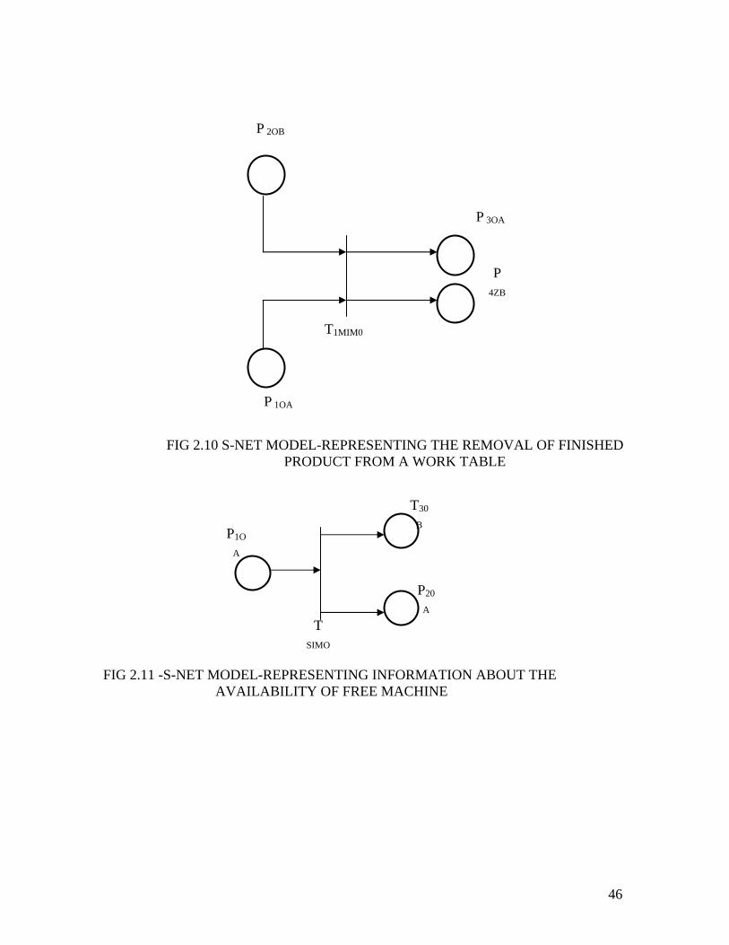
Example IV : Removal of finished product from a worktable (Fig. 2.10)
41

In an automated manufacturing system, a work-piece, comes to the loading station
of an NC Machine from an external world. The barcode reader passes the information
about the Work-piece to the automated computer control system.
The automated control system executes the part program and completes all the
work upon the raw work piece. When the work is over the automated control system
generates a signal and instructs a robot to remove the finished product from the work-
table. Information to the robot for the removal of the finished product and the subsequent
removal of the finished product from the work table etc, are represented conveniently by
a MIMO transition as follows. The place PIOA represents the work-table, and the A colour
token is the finished work piece. P2OB is the input to the robot and the B colour token
signifies the command from the Control system. Firing of MIMO transition is the
operation of removal from the table to the unloading station. P3OA represents the
unloading station. P4zB represents the memory to record the command from the control
system.
Example V : Information about the availability of free machine
In the automated manufacturing system the work piece comes to the loading
station of the NC machine from the external world. Using the barcode, part program and
other operational data, the automated control system completes the job and the finished
product is removed from the table to the unloading stations.
Immediately, an information is passed to the central computer of the automated
control system that the machine is now free and can undertake a new job. Unloading the
finished product to the unloading station and passing the information to the central
computer about the availability of a free machine is represented by a SIMO transition as
follows.(Fig. 2.11)
P1OA is a place representing the robot arm and the A color token in place P1OA,
represents the finished product. TSIMO represents the SIMO transition to indicate the
42

unloading procedure. P2OA represents the unloading station. P3OB represents the input to
the central computer, where the information reaches. B color token in place P3OB,
represents the generated messages.
Example VI: Uploading the part program from the central computer
In an automated manufacturing system, central computer receives a message from
the NC machine, saying that the work is completed and the machine is free, as soon as
the part program is completely executed. When this message reaches the cell controller, it
transfers that part program from the program controller to the cell controller. It afterwards
gets transferred to the central computer. One MIMO transition and one SIMO transition
together as follows in (Fig. 2.12) represent this.
P2OB is a place, which represents the output from the NC machine, and the B color
token represents the message from the machine about the free availability of the machine.
P1OA is the place, which represents the programmable controller. An 'A' color token in
that place represents the part program and operational data. P3OA is the place that
represents the output of the programmable controller. P4OB represents another output of
the programmable controller where the communication to the central computer appears
and B color token represents again the information from the cell controller to upload the
part program to the central computer. Firing of T1MIMO represents the uploading of the
program from the programmable computer to the central controller. P5OA represents the
Data Base Management System where the part program is kept for future use and 'A'
color token there represents the part program. P6ZB is a sink place to accommodate the
token from place P4OB
43

P1S
A
P
2OA
P
3OB
TSIM
O
FIG. 2.7 S-NET MODEL OF A BARCODE READER
P1OA P2ZA
TMIMOP 2OB
P 3OB
FIG 2.8 S-NET MODEL-REPRESENTING THE SELECTION OF PART PROGRAM AND OPERATIONAL DATA IN AN AMS
44

T
3SRT
P2OB
T2OR
D
P
3ZB
TSIM
O
P
1OA
P4O
C
FIG 2.9 S-NET MODEL PRESENTING THE EXECUTION OF PART PROGRAM BY A PROGRAMABLE CONTROLLER
45
T1MIM0
P
4ZB
P 3OA
P 2OB
P 1OA
FIG 2.10 S-NET MODEL-REPRESENTING THE REMOVAL OF FINISHED PRODUCT FROM A WORK TABLE
T30
B
P20
A
P1O
A
T
SIMO
FIG 2.11 -S-NET MODEL-REPRESENTING INFORMATION ABOUT THE AVAILABILITY OF FREE MACHINE
46

P40B
P50A
P30A
47

2.6 Summary
The work contains formal description and a detailed account of the characteristic
of S NET along with several illustrative examples of the various uses of each of the
constituent parts of S NET to prove it’s easiness and conveniences in the area of
modeling. The different types of place nodes, provisions to allow the tokens to allow to
enter the net from external world, making the tokens dead by pushing them into the sink
place etc. are significant features. Transitions association of time and their firing rules are
important aspects as far as the area of the modeling world is concerned. The property of
giving fixed and variable weights to input and output arc are also significant.
APPENDIX
48

A Brief Theory of Bags
Set theory has long been useful in mathematics and computer science. Bag theory
is a natural extension of set theory. A bag, like a set, is a collection of elements over
some domain. However unlike a set, bags allow multiple occurrences of elements. In set
theory , an element is either a member of a set or not a member of a set. In bag theory, an
element, may be in a bag zero times (not in the bag) or one time , two times , or any
specified number of times .
Bag theory has been developed in [Cerf et al. 1971] and [ Peterson 1976 ].
As examples, consider the following bags over the domain {a,b,c,d}:
B1 = {a , b , c }
B2 = {a}
B3 = {a , b , c }
B4 = {a , a , a }
B5 = {b ,c ,b , c }
B6 = {c , c , b , b }
B7 = {a , a , a , a , a , }
Some bags are sets (B1 and B2, for example) . Also, as with sets, the order of the elements
is not important, so B5 and B6 is the same bag. (Ordered bags are sequences.)
In set theory, the basic concepts are a member of relationship. This relationship is
between elements and sets and defines which elements are members of which sets. The
basic concepts of bag theory are the number of occurrences function. This function
defines the number of occurrences of elements in a bag. For an element x in a bag B, we
49

denote the number of occurrences of x in B by #(x, B) (pronounced “the number of x in
B”).
With this conceptual basis, we can define the fundamentals of bag theory. Most of
the concepts and notations are borrowed from set theory in the obvious way. If we restrict
the number of elements in a bag such that 0 ≤ # (x, B) ≤ 1, then set theory results.
1. Membership
The # (x, B) function defines the number of occurrences of an element x in a bag B.
From this it follows that # (x , B ) ≥ 0 For all x and B. We distinguish the zero and
nonzero case. An element x is a number of a bag B. Similarly, if # (x, B) = 0, then
We define the empty bag φ with no members: For all x, #(x ,φ ) = 0.
Cardinality
The cardinality ⏐B⏐ of a bag is the total number of occurrences of elements in the bag:
⏐B⏐=∑#( x , B)
Bag Inclusion and equality
A bag is a sub bag of bag B (denoted by A⊆ B) if every element of A is also an element
of B. at least as many times :
A ⊆ B iff # (x,A) ≤ # (x,B) for all x
Two bags are equal ( A= B ) iff A ⊆ B and B ⊆ A
φ ⊆ B for all bags B
A = B implies ⏐A⏐ = ⏐B⏐
A ⊆ B implies ⏐ A ⏐ = ⏐ B ⏐
50

A bag A is strictely contained in a bag B ( A ⊂ B) if A ⊆ B and A ≠ B . Note that
# ( x ,A) < #(x, B ) does not follow from A ⊂ B, although we do have that ⏐ A ⏐ <
⏐ B ⏐.
References: -
1 Petersion J . L., “ PETRINET THEORY AND MODELLING OF SYSTEMS
“,Printice Hall, 1981.
2 K. S. SIVANANDAN., , ON THE ENHANCE MENT OF TIMED PETRINET
THEORY AND ITS APPLICATIONS TO SOME ASPECTS OF COMPUTER
SYSTEMS” Ph.D Thesis, I I T ROORKEE, 1999.
3 John O. MOODY, Panos J.ANTSAKLIS,. SUPERVISORY CONTROL OF
DISCRETYE EVENT SYSTEMS USING PETRINETS.Kluwer Academic
publishers Boston/Dordrecht/London 1998.
4 N. Viswanatham,. Y. Narahari, PERFORMANCE MODELING OF
AUTOMATED MANUFACTURING SYSTEMS. Prentice-Hall of India Private
Limited NEW DELHI,.1994.
51