S. JOÃO DE LOURE BRIDGE – VULNERABILITY … · stiffness on its structural response was evaluated using the structural analysis software SAP2000. Natural frequencies, ... SAP2000

First Munich Bridge Assessment Conference MBAC 2005

H. Varum, C. Fernandes Munich, 20.-24 June 2005

S. JOÃO DE LOURE BRIDGE – VULNERABILITY ASSESSMENT AND STUDY OF A COMMON STRENGTHENING SOLUTION

Humberto Varum*, Catarina A. L. Fernandes†

* Civil Engineering Department Campus Universitário de Santiago, University of Aveiro, 3810-193 Aveiro, Portugal

[email protected], www.civil.ua.pt

† Civil Engineering Department Campus Universitário de Santiago, University of Aveiro, 3810-193 Aveiro, Portugal

[email protected]

Key words: Bridge assessment, structural vulnerability, strengthening solution.

Abstract. This paper presents a structural vulnerability assessment of the steel bridge S. João de Loure. A structural model of the bridge was created and the influence of the joint’s stiffness on its structural response was evaluated using the structural analysis software SAP2000. Natural frequencies, axial forces and corresponding stress, and maximum mid-span deflection, were analyzed. A common strengthening solution with prestressing cables was studied intending to reduce the bridge’s mid-span deflection.

1

http://www.civil.ua.pt/

mailto:[email protected]

Humberto Varum, Catarina A. L. Fernandes.

1 INTRODUCTION Corrosion is one of the most common problems in steel structures [2]. In the particular case

of a steel bridge, when corrosion affects its joint elements, consequently decreasing the cross-section’s area of these (thus, its axial stiffness), it should be considered the probability of the structural safety of the bridge can be no longer satisfied. Having this in mind, one of the objectives of this work was to evaluate the influence of the joint’s stiffness in the structural response of the steel bridge S. João de Loure. With this purpose, a numerical analysis was performed and the variation of natural frequencies, of axial forces and corresponding stress in the elements, and of the maximum deflection, was analyzed. One other objective of this work, regarding the bridge S. João de Loure, was to analyze a strengthening solution intending to reduce its mid-span deflection.

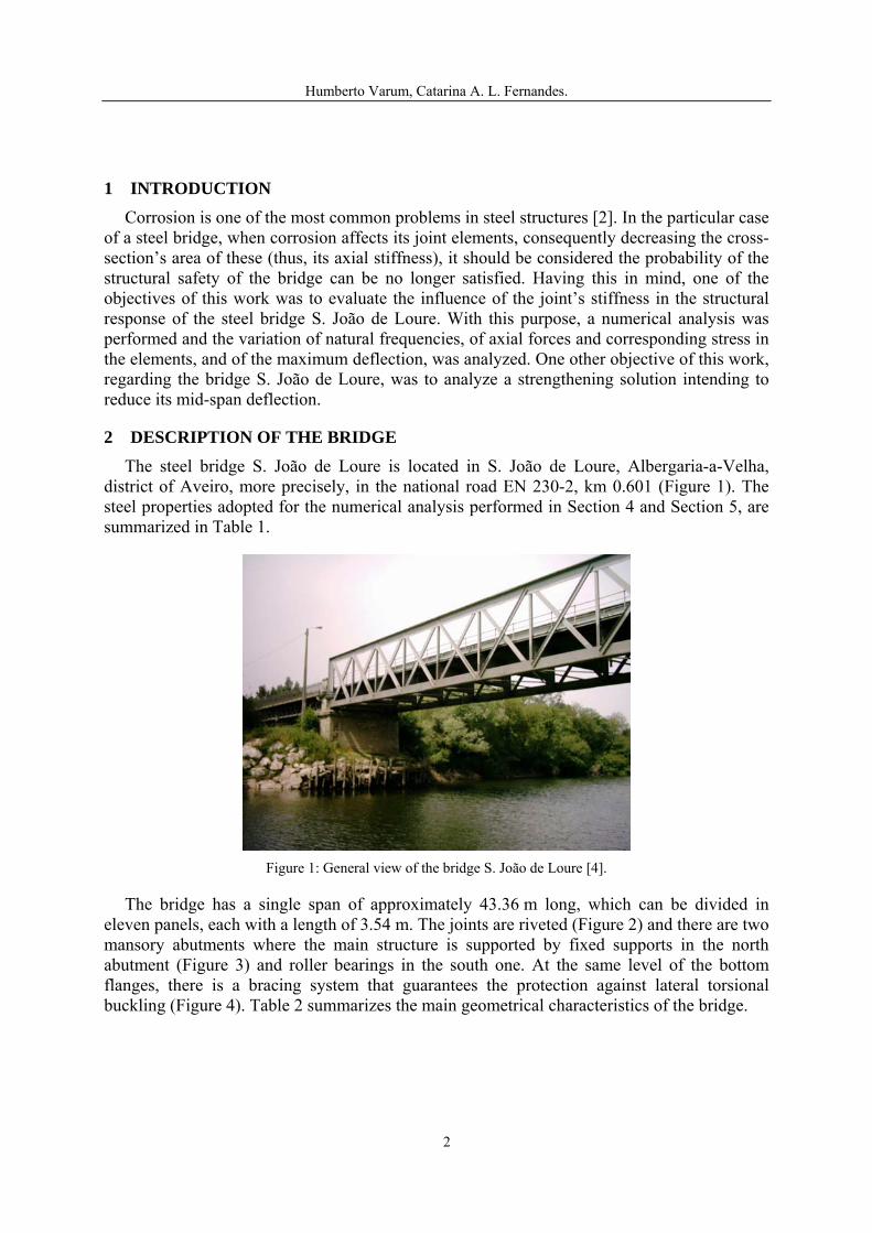
2 DESCRIPTION OF THE BRIDGE The steel bridge S. João de Loure is located in S. João de Loure, Albergaria-a-Velha,

district of Aveiro, more precisely, in the national road EN 230-2, km 0.601 (Figure 1). The steel properties adopted for the numerical analysis performed in Section 4 and Section 5, are summarized in Table 1.

Figure 1: General view of the bridge S. João de Loure [4].

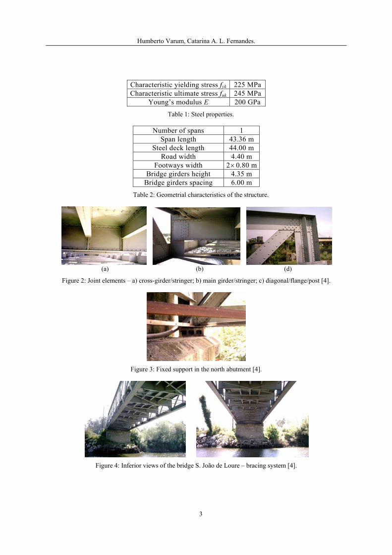
The bridge has a single span of approximately 43.36 m long, which can be divided in eleven panels, each with a length of 3.54 m. The joints are riveted (Figure 2) and there are two mansory abutments where the main structure is supported by fixed supports in the north abutment (Figure 3) and roller bearings in the south one. At the same level of the bottom flanges, there is a bracing system that guarantees the protection against lateral torsional buckling (Figure 4). Table 2 summarizes the main geometrical characteristics of the bridge.

2


Characteristic yielding stress fyk 225 MPa Characteristic ultimate stress fuk 245 MPa

Young’s modulus E 200 GPa

Table 1: Steel properties.

Number of spans 1 Span length 43.36 m

Steel deck length 44.00 m Road width 4.40 m

Footways width 2× 0.80 mBridge girders height 4.35 m

Bridge girders spacing 6.00 m

Table 2: Geometrial characteristics of the structure.

(a) (b) (d) Figure 2: Joint elements – a) cross-girder/stringer; b) main girder/stringer; c) diagonal/flange/post [4].

Figure 3: Fixed support in the north abutment [4].

Figure 4: Inferior views of the bridge S. João de Loure – bracing system [4].

3


3 STRUCTURAL MODEL

3.1 General description The first step in the numerical analysis was to build a 3D structural model of the bridge

(Figure 5), on the structural analysis software SAP2000 [1].

Figure 5: General geometry of the structural model.

A previous model had already been built by Furtado and Marques [4], and the model introduced in this paper is an improvement of that one. In the original model, almost all nodes were hinged, but in the improved model, flanges were considered continuous due to the high stiffness of its joints. Regarding the first objective of this study (study the influence of the joint’s stiffness in the structural response of the bridge), each diagonal and each post were divided in sub-elements. Each bar of length L, representing the diagonals, was divided in three sub-elements (Figure 6): one central sub-element with length L’ and two lateral sub-elements, each one with length Ll. These lateral sub-elements mean to represent the joints and the length Ll was established from the available AutoCAD drawings [7]. For the posts it was adopted the same procedure, but the central sub-element had to be divided in two sub-elements, because an additional node was necessary to apply the loads from the cross-girder.

L = L’+ 2Ll

Ll Ll L’

Figure 6: Improved model: consideration of 3 sub-elements.

3.2 Cross-sections The geometrical characteristics of the element’s cross-sections were calculated from the

AutoCAD drawings [7]. The calculation was made automatically with the numerical tools available, and the cross-section’s area, centre of gravity and moments of inertia, determined

4


for each element, are presented in Table 3. The coordinate axes used for this computation were considered centred in the left inferior point of each cross-section: axis y corresponds to the horizontal axis and axis z to the vertical one. All bars have a uniform cross-section along its length. In Figure 8 is shown the geometry of some element’s cross-sections.

The nomenclature adopted for the cross-sections is shown in Figure 7.

Area Centre of Gravity Moment of Inertia Bridge’s element Label A

(m2) zG (m)

yG (m)

IzG (cm4)

IyG (cm4)

FL 1 0.015870 0.1183 0.2250 9489 36987 FL 2 0.020820 0.0999 0.2250 17842 42779 FL 3 0.025770 0.0907 0.2250 26196 47228 Flanges

FL 4 0.025770 0.0862 0.2250 34549 51072 DIAG 1 0.009823 0.0259 0.1775 16636 811 DIAG 2 0.006510 0.0265 0.1500 8230 561 DIAG 3 0.004680 0.0210 0.1300 4196 293 Diagonals

DIAG 4 0.004076 0.0218 0.1100 2769 225 POST 1 0.029408 0.2564 0.2243 84353 37808 POST 2 0.027096 0.2297 0.2145 80994 11608 POST 3 0.005848 0.1542 0.0750 234 12753 Posts

POST 4 0.003600 0.0491 0.0750 233 932 Cross-girders CGIRD 0.023284 0.3950 0.0985 1497 173655

Stringers STRIN 0.009600 0.2000 0.0890 968 24316 BRAC 1 0.002122 0.0205 0.0710 188 98 Bracing elements BRAC 2 0.001061 0.0205 0.0205 49 49

Table 3: Geometrical characteristics of the element’s cross-sections.

FL 1 FL 2 FL 3 FL 3 FL 4 FL 4

FL 1 FL 2 FL 3 FL 3 FL 4 FL 4

DIAG 1 DIAG 1 DIAG 2 DIAG 3 DIAG 4 DIAG 4

PO

ST 1

PO

ST 2

POST

3

POST

4

POST

5

POST

6

Figure 7: Cross-section’s nomenclature: diagonals, posts and flanges.

5


DIAGONAL

FLANGE

POST

CROSS-GIRDER

STRINGER

Figure 8: Examples of the element’s cross-sections [7].

3.3 Loads and load combinations The dead loads considered in this analysis are the ones that follow: • Weight of the steel structure, automatically evaluated by SAP2000 [1] and multiplied

by 1.1 to account for the fastening’s weight (gusset’s plates, weldings and rivets). • Weight of the concrete slab deck, footways and bridge rails. The values adopted for the density of the materials were: 77 kN/m3 (steel) and 25 kN/m3

(concrete). The live loads considered are the ones mentioned in the Portuguese National Standard [8]

for class I highway bridges and, in this preliminary assessment of the bridge S. João de Loure, the actions corresponding to the wind and earthquake were not taken into account:

• Live load of 4 kN/m2 (Qdistr) uniformly distributed over the deck, plus a transversal load of 50 kN/m acting on every possible position of the deck.

6


• Or, vehicle-type, acting on every possible position of the deck (Qvehicle). • Live load of 3 kN/m2 uniformly distributed on the footways or concentrated load of 20

kN (Qfootway) acting on the bridge rails. Regarding the load combinations, the ultimate limit state combinations considered (ULT 1 and ULT 2) are the following ones:

ULT 1: 1.35G + 1.5 (Qvehicle + Qfootway) (1)

ULT 2: 1.35G + 1.5 (Qdistr + Qfootway) (2)

For each one of these two combinations, different positions for the loads were considered: four positions for the vehicle-type (Qvehicle) in ULT 1, and two positions for the transversal load (Qdistr) in ULT 2.

Concerning the serviceability limit state combinations, the analysis was made for the ones that follow:

SERV 1: G + Ψ1 (Qvehicle + Qfootway), Ψ1 = 0.4 (3)

SERV 2: G + Ψ1 (Qdistr + Qfootway), Ψ1 = 0.4 (4)

In the serviceability limit state combinations, both the vehicle-type and transversal load were applied in the mid-span, which corresponds to the maximum deflection. But for the vehicle-type, two different loading cases were considered: vehicle-type centred in the bridge’s cross-section (SERV 1-A) and vehicle-type with maximum eccentricity in the bridge’s cross-section (SERV 1-B).

4 INFLUENCE OF THE JOINT’S STIFFNESS IN THE STRUCTURAL RESPONSE As previously stated (Section 3.1), each diagonal and each post were divided in three

general sub-elements, with the two lateral ones representing the joints in the corresponding element. Since the objective was to evaluate the influence of the joint’s stiffness in the structural response of the bridge, it was necessary to simulate the variation of this stiffness.

The central sub-elements had an axial stiffness represented by EA (E for the Young’s modulus and A for the area of the cross-section of the central sub-element). The lateral sub-element’s axial stiffness was represented by EANL (A for the area of the cross-section of the lateral sub-elements). The axial stiffness EANL was varied in the range [0.5EA ; 1.5EA], simulating possible variations of the area caused by, for example, corrosion. The structural response was then evaluated for the following values of EANL: 0.5EA, 0.6EA, 0.7EA, 0.8EA, 0.9EA, 1.0EA, 1.1EA, 1.2EA, 1.3EA, 1.4EA and1.5EA. For each case, were analyzed:

• Natural frequencies. • Maximum axial forces in the elements and corresponding maximum stress. • Maximum deflection.

7


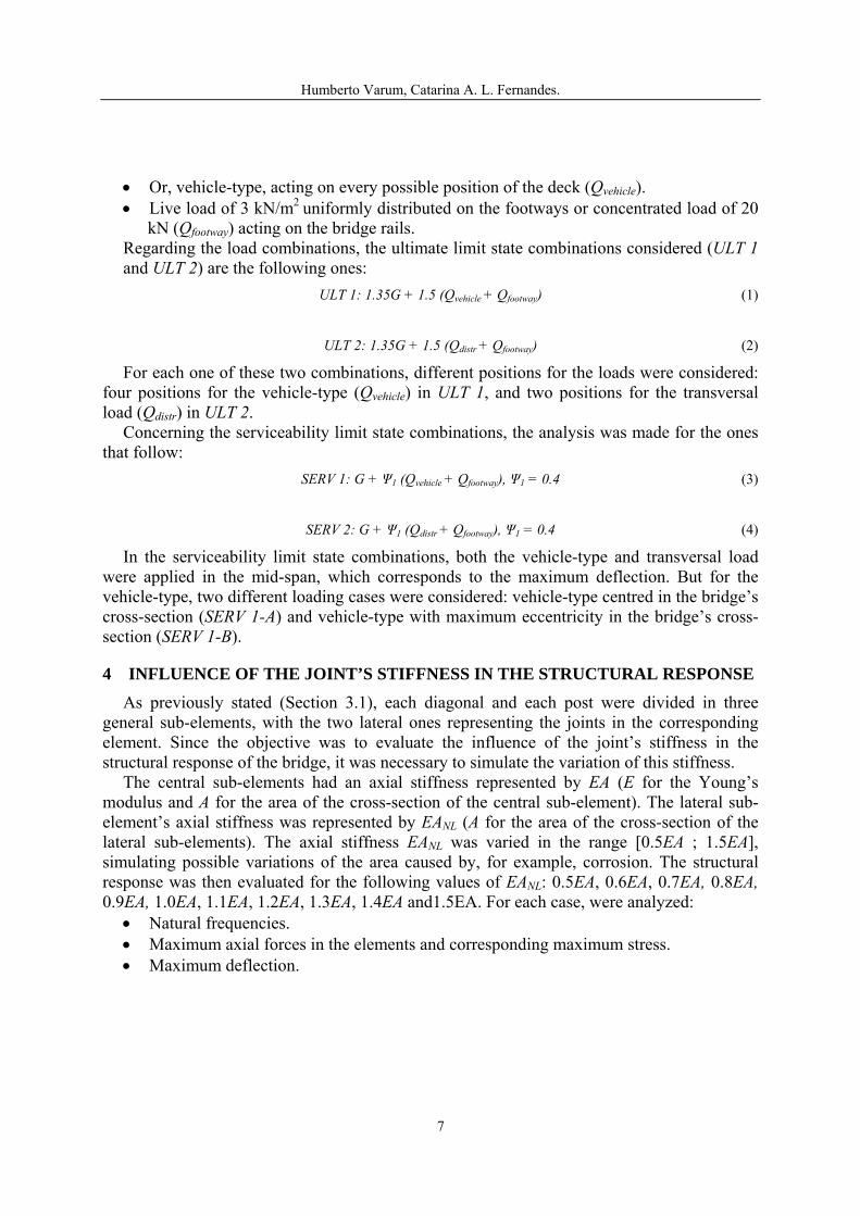
4.1 Numerical results (1): natural frequencies The analysis was made for the first 16 vibration modes. Table 4 describes each vibration

mode and presents the corresponding natural frequencies of the structure, calculated by SAP2000 [1] for EANL = EA. Since the natural frequencies did not show a significant variation for each value of EANL, the frequencies calculated for EANL = EA can be considered valid for all the values of EANL in the range [0.5EA ; 1.5EA].

FrequenciesVibration modes f (Hz)

1 Transversal bending of

the overall structure 2.12


the main girders 2.97

3 a 13

Local bending of the bracing elements 3.03


the overall structure 3.90

15

Transversal bending of the overall structure 5.03

16 In-plane bending of the

overall structure 5.18

X

YY

Z XZ

XOY

X

YY

Z XZ

XOY

XYY

Z

X

Z

3D

X

Y

XZ

Y

Z XOY

X

Y

XZ

Y

Z

XOY

X

Z

XOZ

Table 4: Vibration modes and corresponding frequencies.

4.2 Numerical results (2): maximum axial forces and corresponding stress

The maximum axial force, Nmax, and corresponding maximum stress, maxσ , in the elements, calculated for the ultimate limit state combinations, are presented in Table 5. The diagonal and the post with maximum stress are located in the panel nearest to the supports. As expected, the upper and bottom flanges with the maximum stress are located in the central panel.

Diagonal Post Upper flange Bottom flange

EANL/EA Nmax (kN)

σmax (MPa)

Nmax (kN)

σmax (MPa)

Nmax (kN)

σmax (MPa)

Nmax (kN)

σmax (MPa)

0.5 -855.44 -174.17 -690.13 -46.93 -3401.44 -131.99 3300.13 128.060.6 -854.95 -145.06 -690.79 -39.15 -3406.27 -132.18 3302.16 128.140.7 -854.52 -124.27 -691.32 -33.58 -3409.84 -132.32 3303.80 128.20

8


0.8 -854.15 -108.69 -691.75 -29.40 -3412.59 -132.42 3305.00 128.250.9 -853.83 -96.58 -692.11 -26.15 -3414.77 -132.51 3305.90 128.281 -853.56 -86.89 -692.42 -23.55 -3416.55 -132.58 3306.61 128.31

1.1 -853.31 -78.97 -692.68 -21.41 -3418.02 -132.64 3307.17 128.331.2 -853.10 -72.37 -692.90 -19.63 -3419.27 -132.68 3307.63 128.351.3 -852.92 -66.79 -693.10 -18.13 -3420.33 -132.73 3308.01 128.371.4 -852.75 -62.01 -693.27 -16.84 -3421.26 -132.76 3308.33 128.381.5 -852.60 -57.86 -693.42 -15.72 -3422.06 -132.79 3308.60 128.39

Table 5: Maximum axial forces and corresponding maximum stress.

The maximum stress surges at the diagonal, for EANL = 0.5EA, and is equal to 174.17 MPa.

Consequently, and not considering the effect of local or global instability, the structural safety was verified, according the Portuguese standards [9]:

maxσ = 174.17 MPa < fyd = fyk / 1.1 = 225 / 1.1 = 204.55 MPa (5)

The evolution of the maximum axial force and corresponding stress for each element, function of the axial stiffness, is shown in Figure 9 and Figure 10.

-856

-855

-854

-853

-852

-8510.5 0.6 0.7 0.8 0.9 1 1.1 1.2 1.3 1.4 1.5

-694

-693

-692

-691

-690

-689

-6880.5 0.6 0.7 0.8 0.9 1 1.1 1.2 1.3 1.4 1.5

-3430

-3420

-3410

-3400

-33900.5 0.6 0.7 0.8 0.9 1 1.1 1.2 1.3 1.4 1.5

3300

3302

3304

3306

3308

3310

0.5 0.6 0.7 0.8 0.9 1 1.1 1.2 1.3 1.4 1.5

Nm

ax (k

N)

Nm

ax (k

N)

Nm

ax (k

N)

Nm

ax (k

N)

EANL/EA EANL/EA

EANL/EA

EANL/EA

Diagonal Post

Upper flange Bottom flange

Figure 9: Maximum axial forces in the elements function of the axial stiffness.

9


-180

-140

-100

-60

-200.5 0.6 0.7 0.8 0.9 1 1.1 1.2 1.3 1.4 1.5

-60

-45

-30

-15

0.5 0.6 0.7 0.8 0.9 1 1.1 1.2 1.3 1.4 1.5

0

-300

-250

-200

-150

-100

-50

00.5 0.6 0.7 0.8 0.9 1 1.1 1.2 1.3 1.4 1.5

0

50

100

150

200

250

300

0.5 0.6 0.7 0.8 0.9 1 1.1 1.2 1.3 1.4 1.5

σ max

(MPa

)

σ max

(MPa

)

σ max

(MPa

)

σ max

(MPa

)

EANL/EA

EANL/EA

Diagonal Po


st

Figure 10: Maximum stress in the elements, function of the axial stiffness.

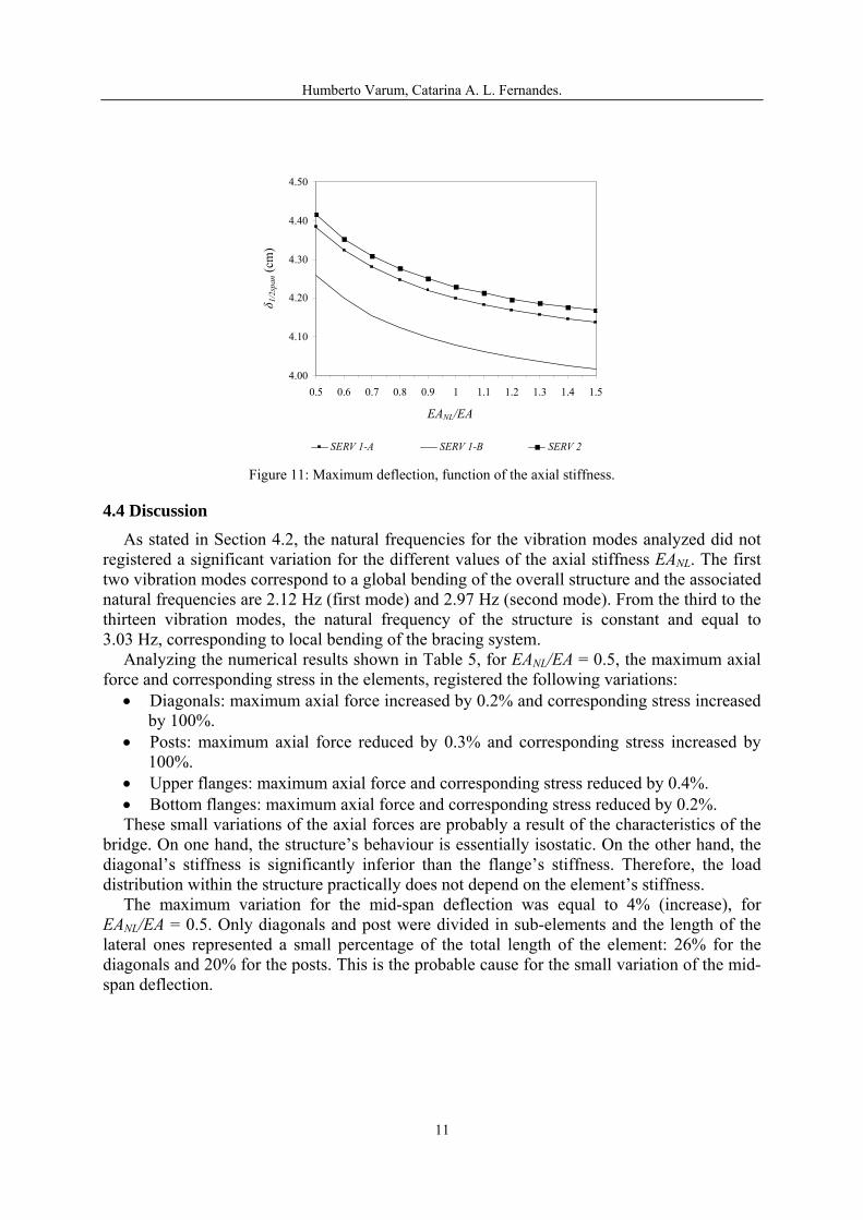
4.3 Numerical results (3): maximum deflection The maximum deflection, δ1/2span, located in the central panel (mid-span), was calculated

for the serviceability limit state combinations. The combination SERV 2 gives the maximum values, as shown in Table 6 and in Figure 11.

δ1/2span (cm) EANL/EA

SERV 1-A SERV 1-B SERV 2 0.5 4.38 4.26 4.42 0.6 4.32 4.20 4.35 0.7 4.28 4.16 4.31 0.8 4.25 4.12 4.28 0.9 4.22 4.10 4.25 1 4.20 4.08 4.23

1.1 4.18 4.06 4.21 1.2 4.17 4.05 4.20 1.3 4.16 4.04 4.19 1.4 4.15 4.02 4.18 1.5 4.14 4.02 4.17

Table 6: Maximum deflection.

10


4.00

4.10

4.20

4.30

4.40

4.50

0.5 0.6 0.7 0.8 0.9 1 1.1 1.2 1.3 1.4 1.5

SERV 1-A SERV 1-B SERV 2

EANL/EA

δ 1/2

span

(cm

)

Figure 11: Maximum deflection, function of the axial stiffness.

4.4 Discussion As stated in Section 4.2, the natural frequencies for the vibration modes analyzed did not

registered a significant variation for the different values of the axial stiffness EANL. The first two vibration modes correspond to a global bending of the overall structure and the associated natural frequencies are 2.12 Hz (first mode) and 2.97 Hz (second mode). From the third to the thirteen vibration modes, the natural frequency of the structure is constant and equal to 3.03 Hz, corresponding to local bending of the bracing system.

Analyzing the numerical results shown in Table 5, for EANL/EA = 0.5, the maximum axial force and corresponding stress in the elements, registered the following variations:

• Diagonals: maximum axial force increased by 0.2% and corresponding stress increased by 100%.

• Posts: maximum axial force reduced by 0.3% and corresponding stress increased by 100%.

• Upper flanges: maximum axial force and corresponding stress reduced by 0.4%. • Bottom flanges: maximum axial force and corresponding stress reduced by 0.2%. These small variations of the axial forces are probably a result of the characteristics of the

bridge. On one hand, the structure’s behaviour is essentially isostatic. On the other hand, the diagonal’s stiffness is significantly inferior than the flange’s stiffness. Therefore, the load distribution within the structure practically does not depend on the element’s stiffness.

The maximum variation for the mid-span deflection was equal to 4% (increase), for EANL/EA = 0.5. Only diagonals and post were divided in sub-elements and the length of the lateral ones represented a small percentage of the total length of the element: 26% for the diagonals and 20% for the posts. This is the probable cause for the small variation of the mid-span deflection.

11


5 STRENGTHENING SOLUTION FOR THE BRIDGE S. JOÃO DE LOURE With a view to reduce the mid-span deflection of the bridge S. João de Loure, a

strengthening solution with prestressing cables, illustrated in Figure 12, was analyzed. It was used the structural model described in Section 3, with EANL = EA.

Prestressing cable

Figure 12: Strengthening scheme.

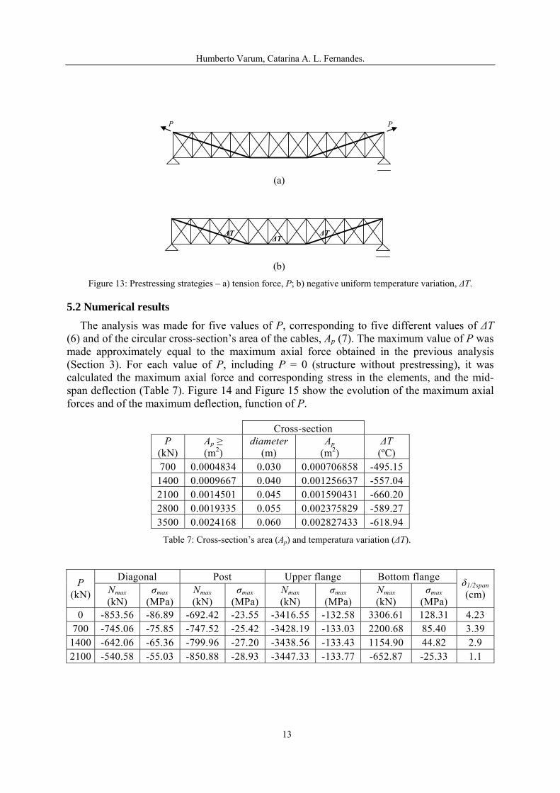
5.1 Prestressing simulation The usual way to simulate the prestressing is to apply a tension force, P, in each extremity

of the cable (Figure 13-a). However, this solution is considered more suitable for the cases in which the prestressing is applied, for example, inside a concrete element. For this study, it was chosen to apply a negative uniform temperature variation, ΔT, on the prestressing cables (Figure 13-b). Subjected to a negative temperature, the cables tend to get shorter, becoming tensioned as a result of the opposition to that deformation.

The temperature variation was calculated using equation (6):

p

NTEA α

Δ = (6)

N is the prestressing force (equal to the tension force, P), E is the Young’s modulus of the prestressing steel (200 GPa), Ap is the cross-section’s area of the cable (7) and α is the thermal expansion coefficient of the prestressing steel ( 51 10−× ).

ppd

NAf

≥ (7)

pkpd

ff 0.9

1.1=

(8)

In equation (7), fpd is the design value of the yielding stress of the prestressing cable, calculated from equation (8), where fpk is the characteristic value of the stress (1770 MPa).

12


(a)

(b)

P P

ΔT ΔT ΔT

Figure 13: Prestressing strategies – a) tension force, P; b) negative uniform temperature variation, ΔT.

5.2 Numerical results The analysis was made for five values of P, corresponding to five different values of ΔT

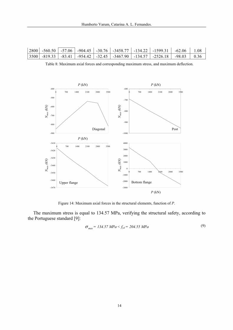
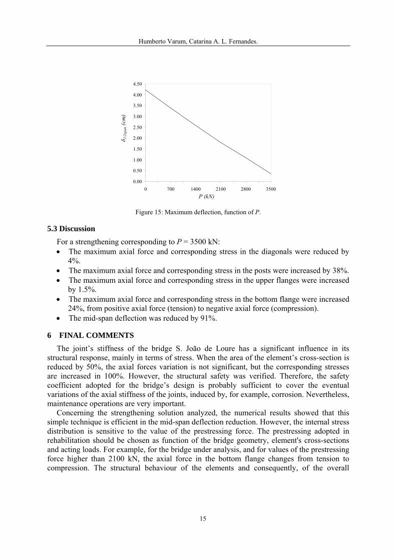
(6) and of the circular cross-section’s area of the cables, Ap (7). The maximum value of P was made approximately equal to the maximum axial force obtained in the previous analysis (Section 3). For each value of P, including P = 0 (structure without prestressing), it was calculated the maximum axial force and corresponding stress in the elements, and the mid-span deflection (Table 7). Figure 14 and Figure 15 show the evolution of the maximum axial forces and of the maximum deflection, function of P.

Cross-section

P (kN)

Ap ≥ (m2)

diameter (m)

Ap (m2)

ΔT (ºC)

700 0.0004834 0.030 0.000706858 -495.15 1400 0.0009667 0.040 0.001256637 -557.04 2100 0.0014501 0.045 0.001590431 -660.20 2800 0.0019335 0.055 0.002375829 -589.27 3500 0.0024168 0.060 0.002827433 -618.94

Table 7: Cross-section’s area (Ap) and temperatura variation (ΔT).

Diagonal Post Upper flange Bottom flange P

(kN) Nmax (kN)

σmax (MPa)

Nmax(kN)

σmax (MPa)

Nmax(kN)

σmax (MPa)

Nmax(kN)

σmax (MPa)

δ1/2span (cm)

0 -853.56 -86.89 -692.42 -23.55 -3416.55 -132.58 3306.61 128.31 4.23 700 -745.06 -75.85 -747.52 -25.42 -3428.19 -133.03 2200.68 85.40 3.39

1400 -642.06 -65.36 -799.96 -27.20 -3438.56 -133.43 1154.90 44.82 2.9 2100 -540.58 -55.03 -850.88 -28.93 -3447.33 -133.77 -652.87 -25.33 1.1

13


2800 -560.50 -57.06 -904.45 -30.76 -3458.77 -134.22 -1599.31 -62.06 1.08 3500 -819.33 -83.41 -954.42 -32.45 -3467.90 -134.57 -2526.18 -98.03 0.36

Table 8: Maximum axial forces and corresponding maximum stress, and maximum deflection.

-900

-800

-700

-600

-500

-4000 700 1400 2100 2800 3500

-1000

-900

-800

-700

-6000 700 1400 2100 2800 3500

-3470

-3460

-3450

-3440

-3430

-3420

-34100 700 1400 2100 2800 3500

-3000

-2000

-1000

0

1000

2000

3000

4000

0 700 1400 2100 2800 3500

Nm

ax (k

N)

Nm

ax (k

N)

Nm

ax (k

N)

Nm

ax (k

N)

P (kN) P (kN)

P (kN)

P (kN)

Diagonal Post


Figure 14: Maximum axial forces in the structural elements, function of P.

The maximum stress is equal to 134.57 MPa, verifying the structural safety, according to the Portuguese standard [9]:

maxσ = 134.57 MPa < fyd = 204.55 MPa (9)

14


0.00

0.50

1.00

1.50

2.00

2.50

3.00

3.50

4.00

4.50

0 700 1400 2100 2800 3500

P (kN)

δ 1/2

span

(cm

)

Figure 15: Maximum deflection, function of P.

5.3 Discussion For a strengthening corresponding to P = 3500 kN: • The maximum axial force and corresponding stress in the diagonals were reduced by

4%. • The maximum axial force and corresponding stress in the posts were increased by 38%. • The maximum axial force and corresponding stress in the upper flanges were increased

by 1.5%. • The maximum axial force and corresponding stress in the bottom flange were increased

24%, from positive axial force (tension) to negative axial force (compression). • The mid-span deflection was reduced by 91%.

6 FINAL COMMENTS The joint’s stiffness of the bridge S. João de Loure has a significant influence in its

structural response, mainly in terms of stress. When the area of the element’s cross-section is reduced by 50%, the axial forces variation is not significant, but the corresponding stresses are increased in 100%. However, the structural safety was verified. Therefore, the safety coefficient adopted for the bridge’s design is probably sufficient to cover the eventual variations of the axial stiffness of the joints, induced by, for example, corrosion. Nevertheless, maintenance operations are very important.

Concerning the strengthening solution analyzed, the numerical results showed that this simple technique is efficient in the mid-span deflection reduction. However, the internal stress distribution is sensitive to the value of the prestressing force. The prestressing adopted in rehabilitation should be chosen as function of the bridge geometry, element's cross-sections and acting loads. For example, for the bridge under analysis, and for values of the prestressing force higher than 2100 kN, the axial force in the bottom flange changes from tension to compression. The structural behaviour of the elements and consequently, of the overall

15


structure, corresponding to different levels of prestressing, can be very different, in terms of internal stress distribution and deformations for different loading cases.

7 ACKNOLEDGEMENTS The authors would like to acknowledge the Junta Autónoma de Estradas, for the

information provided for this study. REFERENCES [1] SAP2000 Nonlinear 8.15. Computer and Structures, Inc., 2003.

[2] P. Brinckerhoff. Bridge inspection and rehabilitation. Ed. Louis G. Silano, P.E. ISBN 0-471-53262-2, 1993.

[3] P.C.M. Freire, M.R.F. Martins and M.T.P. Torres. Steel highway bridges. Junta Autónoma de Estradas, 1998 (in portuguese).

[4] A.C. Furtado and A. Marques. Maintenance and rehabilitation assessment of the S. João de Loure bridge –Vouga's river. Civil Engineering Department, University of Aveiro, Aveiro, Portugal, 2003 (in portuguese).

[5] H. Varum. Seismic assessment, strengthening and repair of existing buildings. PhD Thesis, University of Aveiro, Aveiro, Portugal, 2003.

[6] C. Fernandes and H. Silva. Bridge's evaluation, maintenance and strengthening. Civil Engineering Department, University of Aveiro, Aveiro, Portugal, 2004 (in portuguese).

[7] S. João de Loure bridge – Drawings (AutoCAD format). 2001.

[8] RSA – Regulamento de Segurança e Acções para Estruturas de Edifícios e Ponte. Decreto de Lei nº 235/83, 31 May, 1983 (in portuguese).

[9] REAE – Regulamento de Estruturas de Aço para Edifícios. Decreto de Lei nº 211/86, 31 July, 1986 (in portuguese).

[10] C. Fernandes and H. Varum. Vulnerability assessment of the S. João de Loure bridge – Vouga’s river. Proceedings of the 4th International Workshop on Life-Cycle Cost Analysis and Design of Civil Infrastructure Systems, 8-11 May, Cocoa Beach, Florida, EUA, 2005.

16

Documents

S. JOÃO DE LOURE BRIDGE – VULNERABILITY … · stiffness on its structural response was evaluated using the structural analysis software SAP2000. Natural frequencies, ... SAP2000