Commonwealth of Pennsylvania

STATE IMPLEMENTATION PLAN REVISION:

ATTAINMENT DEMONSTRATION AND BASE

YEAR INVENTORY PENNSYLVANIA PORTION OF THE

PHILADELPHIA-WILMINGTON, PA-NJ-DE FINE PARTICULATE NONATTAINMENT AREA

APRIL 2010

Bureau of Air Quality Pennsylvania Department of Environmental Protection

P.O. Box 8468 Harrisburg, PA 17105-8468

717-787-9495

www.depweb.state.pa.us

John Hanger Secretary

Edward G. Rendell Governor

blank for two-sided copying

Table of Contents Executive Summary ............................................................................................................. i I. INTRODUCTION AND OVERVIEW.......................................................................... 1

A. Health and Environmental Effects of Fine Particulate Matter (PM2.5) .............. 1 B. Sources of PM2.5 and Implications for Reduction................................................. 1 C. Purpose and Structure of this Document............................................................... 4 D. Public Participation ................................................................................................. 5

II. NATURE OF THE PROBLEM IN THE PHILADELPHIA AREA ............................ 6 A. Background ............................................................................................................. 6 B. Air Quality Monitoring Trends Analysis .............................................................. 7

1. Design Value Trend ............................................................................................... 7 2. NO2 Monitoring Trend........................................................................................... 9 3. SO2 Monitoring Trend ......................................................................................... 10

C. Seasonal Variability .............................................................................................. 10 1. FRM Monitoring Trends...................................................................................... 10 2. Speciation Monitoring Trends ............................................................................. 11

III. EMISSION INVENTORIES ..................................................................................... 12 A. Summary of 2002 Emissions ................................................................................ 12 B. Summary of Inventory Methodologies ................................................................ 13 C. Projected Inventories ............................................................................................ 16

1. Summary of 2009 Estimated Emissions .............................................................. 16 2. Growth Projection Methodologies....................................................................... 16

D. Reasonable Further Progress (RFP) Requirements .......................................... 20 E. Motor Vehicle Emission Budgets for Transportation Conformity................... 20

IV. CONTROL STRATEGIES ....................................................................................... 23 A. Permanent and Enforceable Control Measures ................................................. 23

1. Stationary Point Sources ...................................................................................... 23 2. Highway Vehicle Sources.................................................................................... 26 3. Nonroad Sources.................................................................................................. 29

B. Reasonably Available Control Measures/Reasonably Available Control Technology Analysis ................................................................................................... 29 C. Other Measures - VOC Control Measures ......................................................... 31

V. ATTAINMENT DEMONSTRATION AND WEIGHT OF EVIDENCE (WOE)..... 33 A. Attainment Demonstration Background and Objectives .................................. 33 B. Philadelphia Area Conceptual Model Description............................................. 34 C. Modeling Domain and Photochemical Modeling System .................................. 36 D. Model Performance Evaluation ........................................................................... 38

1. Daily PM2.5 Mass ................................................................................................. 38 2. PM2.5 Speciation................................................................................................... 40

E. Projected 2009 Design Values for the Philadelphia Nonattainment Area ....... 42 1. Overview............................................................................................................... 42 2. Modeled Attainment Test .................................................................................... 42 3. Determine Baseline Design Values ..................................................................... 43 4. Relative Response Factor Calculations................................................................ 45 5. Annual SMAT Results......................................................................................... 46 6. 24-Hour SMAT Results ....................................................................................... 48

F. Unmonitored Area Analysis............................................................................... 49

G. Local Area Analysis .............................................................................................. 50 H. Weight of Evidence and Other Documentation Supporting Attainment ........ 53 I. Conclusions ............................................................................................................. 56

VI. CONTINGENCY MEASURES FOR THE ATTAINMENT DEMONSTRATION 57 A. Contingency Measure Requirement.................................................................... 57 B. Identified Contingency Measures ........................................................................ 58

ACRONYMS AND ABBREVIATIONS......................................................................... 63

Table of Tables

Table E-1: Summary of the Five-County Philadelphia Area Direct PM and

Precursor Emissions (Tons per Year) .................................................................... iii Table II-1: Philadelphia Area PM2.5 Annual Average and Design Values (µg/m3) ... 7 Table III-1: 2002 Annual Emissions (Tons per Year) ................................................ 13 Table III-2: 2009 Projected Emissions (Tons per Year)............................................. 16 Table III-3: Five-County Philadelphia Area VMT and Emissions .......................... 18 Table III-4 Comparison of 2009 On-Road Mobile Precursor Emissions to the Total

Projected 2009 Inventory ....................................................................................... 21 Table III-5: Motor Vehicle Emission Budgets............................................................. 22 Table IV-1: Summary of Emission Reductions 2002-2009 from Control Measures23 Table V-1: Annual PM2.5 Quarterly RRF Values ........................................................ 47 Table V-2: Annual SMAT Results for the Philadelphia Area 2009 On The Books/On

The Way Control Measures ................................................................................... 47 Table V-3: 24-hour PM2.5 Quarterly RRF Values ....................................................... 48 Table V-4: 24-hour SMAT Results for the Philadelphia Area 2009 On The

Books/On The Way Control Measures ................................................................. 49 Table V-5: Summary of Large PM2.5 Sources near the Chester Monitor.................. 51 Table V-6: Summary of PM2.5 Weight of Evidence Guidelines (EPA Guidance)..... 53 Table VI-1: Changes in Design Value and Emissions Expected by 2009.................. 57 Table VI-2: Calculation of Required and Excess Emissions Reductions ................. 58 Table VI-3: Calculation of Required Contingency Plan Reductions ........................ 58

Table of Figures

Figure E-1: Map of the Philadelphia-Wilmington, PA-NJ-DE Nonattainment Areaii Figure 1: PM2.5 Annual Average and Design Value Trends......................................... 8 Figure 2: NO2 Monitoring Trend ................................................................................... 9 Figure 3: SO2 Monitoring Trend .................................................................................. 10 Figure 4: Pennsylvania’s PM2.5 Nonattainment Areas ............................................... 34 Figure 5: Philadelphia Area Percentage of Total Mass.............................................. 36 Figure 6. OTC Modeling Study Domain...................................................................... 37 Figure 7: Mean Fractional Error ................................................................................. 39 Figure 8: Mean Fractional Bias .................................................................................... 40 Figure 9: Time Series of SO4 Mass ............................................................................... 41 Figure 10. Wind Rose: Philadelphia Int’l Airport Location (2004-2008)................. 52 Figure 11: Philadelphia Area PM2.5 Trends ................................................................ 55

APPENDICES

APPENDIX A: AIR QUALITY MONITORING INFORMATION A-1 United States Environmental Protection Agency Air Quality System Quick Look:

Pennsylvania (1999-2008) A-2 United States Environmental Protection Agency Air Quality System: Quarterly PM2.5

Data (1999-2008) APPENDIX B: STATIONARY POINT SOURCES

B-1 Methodology – Preparation of Pennsylvania Point Source Inventories and Instructions for Completing the Annual Emissions Reporting Forms

B-2 Facility Annual Emissions B-3 Banked Emissions Reduction Credits

APPENDIX C: STATIONARY AREA SOURCES C-1 Pennsylvania 2002 Area Source Criteria Air Pollutant Emission Estimation Methods

(EH Pechan, Feb. 2004) C-2 Area Source Annual Emissions

APPENDIX D: EMISSIONS PROJECTIONS D-1 Development of Emission Projections for 2009, 2012, and 2018 for NonEGU Point,

Area and Nonroad Sources in the MANE-VU Region (MACTEC, Feb. 2007) D-2 Documentation of 2018 Emissions from Electric Generating Units in the Eastern

United States for MANE-VU’s Regional Haze Modeling (Alpine Geophysics, April 2008)

D-3 Future Year Electricity Generating Sector Emission Inventory Development Using the Integrated Planning Model (IPM®) in Support of Fine Particulate Mass and Visibility Modeling in the VISTAS and Midwest RPO Regions (ICF, April 2005)

APPENDIX E: HIGHWAY VEHICLE SOURCES INVENTORY INFORMATION E-1 Mobile Source Highway Emissions Inventory – An Explanation of Methodology E-2 Highway Emissions Estimates E-3 MOBILE6.2 Input Parameter Summary E-4 MOBILE6.2 Sample Input File E-5 Traffic Growth Forecasting System Report

APPENDIX F: NONROAD SOURCES F-1 Emissions Estimation Methodology F-2 Nonroad Source Emissions F-3 Philadelphia International Airport Inventory and Methodology F-4 Capacity Enhancement Program Construction Period Air Emissions Inventory

APPENDIX G: REASONABLY AVAILABLE CONTROL MEASURES G-1 Identification and Evaluation of Candidate Control Measures, Final Technical

Support Document (MACTEC, Feb. 2007) G-2 OTC Initial List of Measures (Appendix B of Candidate Control Measures TSD) G-3 Assessment of Reasonable Progress for Regional Haze in MANE-VU Class I Areas

(MACTEC, July 2007) APPENDIX H: MODELING DEMONSTRATION

H-1 CMAQ Model Performance and Assessment for Base Year 2002 PM2.5 Mass and Speciation (NY DEC, Dec. 2007)

H-2 Meteorological Modeling of 2002 Using Penn State/NCAR 5th Generation Mesoscale Model (MM5) (NY DEC, Mar. 2006)

H-3 Processing of 2002 Anthropogenic Emissions: OTC Regional and Urban 12km Base Year Simulation (NY DEC, Mar. 2007)

H-4 PM2.5 Modeling Using the SMOKE/CMAQ System Over the Ozone Transport Region (OTR) (NY DEC, Feb. 2006)

H-5 Processing of 2002 Biogenic Emissions for OTC / MANE-VU Regional and Urban Modeling (NY DEC, Sep. 2006)

H-6 Final Air-Quality Modeling Protocol for the Annual PM2.5 NAAQS: Philadelphia-Wilmington, PA-NJ-DE Annual PM2.5 Nonattainment Area (PA DEP, Oct. 2007)

H-7 Sample Calculation of Projected 2009 PM2.5 Annual and 24-hour Concentrations

- i -

Executive Summary

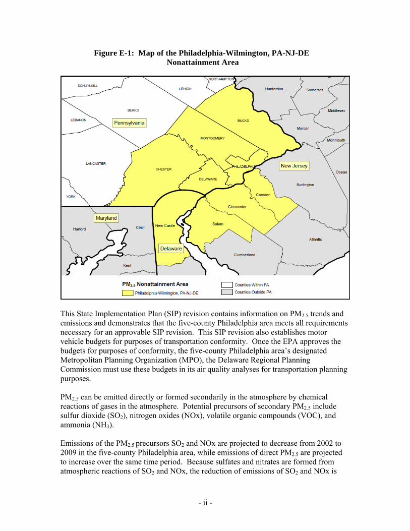
Particulate matter is a mixture of microscopic solids and liquid droplets suspended in air that include: acids (such as nitrates and sulfates), organic chemicals, metals, soil or dust particles and allergens (such as fragments of pollen or mold spores). Fine particle pollution or PM2.5 describes particulate matter that is less than or equal to 2.5 micrometer (μm) in diameter, approximately 1/30th the diameter of a human hair. Health studies have shown a significant association between exposure to fine particles and premature death from heart or lung disease. Fine particles can aggravate heart and lung diseases and have been linked to effects such as cardiovascular symptoms, cardiac arrhythmias, heart attacks, respiratory symptoms, asthma attacks, and bronchitis. These effects can result in increased hospital admissions, emergency room visits, absences from school or work, and restricted activity days. Individuals that may be particularly sensitive to fine particle exposure include people with heart or lung disease, older adults, and children. The United States Environmental Protection Agency (EPA) issued fine particle (PM2.5) national ambient air quality standards (NAAQS) in 1997 after evaluating hundreds of health studies and conducting an extensive peer review process. The EPA established an annual primary (health-based) and secondary (welfare-based) standard of 15.0 micrograms per cubic meter (μg/m3), based on the 3-year average of annual mean PM2.5 concentrations. The EPA also established a primary and secondary 24-hour standard of 65 μg/m3 determined by the 3-year average of the 98th percentile of 24-hour concentrations. On December 17, 2004, the EPA issued air quality designations for the PM2.5 standard based on air quality monitoring data from 2001-2003. The final designations were published in the Federal Register on January 5, 2005 (70 FR 944). The designations became effective on April 5, 2005. On April 5, 2005, the EPA issued a supplemental notice changing the designation of certain areas from nonattainment to attainment based on newly available air quality data (70 FR 19844; published in the Federal Register on April 14, 2005). The EPA designated eight areas in Pennsylvania as PM2.5 nonattainment areas, comprising all or parts of 21 Pennsylvania counties. The Philadelphia-Wilmington, PA-NJ-DE Nonattainment Area (Philadelphia Area) is comprised of 9 counties in Pennsylvania, New Jersey and Delaware. The Philadelphia Area is required to attain the PM2.5 NAAQS no later than five years from the effective date of designation, or April 5, 2010. Bucks, Chester, Delaware, Montgomery and Philadelphia counties (five-county Philadelphia area) in Pennsylvania are included in the Philadelphia Area. Figure E-1 displays a map of the Philadelphia Area.

- ii -

Figure E-1: Map of the Philadelphia-Wilmington, PA-NJ-DE Nonattainment Area

This State Implementation Plan (SIP) revision contains information on PM2.5 trends and emissions and demonstrates that the five-county Philadelphia area meets all requirements necessary for an approvable SIP revision. This SIP revision also establishes motor vehicle budgets for purposes of transportation conformity. Once the EPA approves the budgets for purposes of conformity, the five-county Philadelphia area’s designated Metropolitan Planning Organization (MPO), the Delaware Regional Planning Commission must use these budgets in its air quality analyses for transportation planning purposes. PM2.5 can be emitted directly or formed secondarily in the atmosphere by chemical reactions of gases in the atmosphere. Potential precursors of secondary PM2.5 include sulfur dioxide (SO2), nitrogen oxides (NOx), volatile organic compounds (VOC), and ammonia (NH3). Emissions of the PM2.5 precursors SO2 and NOx are projected to decrease from 2002 to 2009 in the five-county Philadelphia area, while emissions of direct PM2.5 are projected to increase over the same time period. Because sulfates and nitrates are formed from atmospheric reactions of SO2 and NOx, the reduction of emissions of SO2 and NOx is

- iii -

expected to result in attainment of the PM2.5 air quality standard in the Philadelphia Area. Based on speciated data from the Chester monitor, sulfates and nitrates account for 46% of the PM2.5 mass in the Philadelphia Area. The emission projections take into account both growth in economic activity that increases emissions and control measures implemented to reduce emissions.

Table E-1: Summary of the Five-County Philadelphia Area Direct PM and Precursor Emissions (Tons per Year)

Pollutant 2002 2009

PM2.5 14727 15219

PM10 61758 66035

SO2 40459 28200 NOx 120248 91651 VOC 122973 101834

NH3 7705 9239

The permanent and enforceable control measures that enable the Pennsylvania portion of the Philadelphia Area to demonstrate attainment of the PM2.5 NAAQS include:

The Clean Air Interstate Rule (CAIR) and the NOx “SIP Call” reducing interstate pollution transport;

State regulation of smaller sources of NOx, cement kilns and large stationary internal combustion engines;

The Pennsylvania and federal new motor vehicle emission control programs for passenger and light-duty trucks;

The Pennsylvania and federal heavy-duty diesel emission control programs; Federal fuel programs for highway vehicles and nonroad mobile equipment; and Federal regulation of offroad diesel and gasoline-powered vehicles and

equipment.

In addition, Pennsylvania’s Diesel-Powered Motor Vehicle Idling Act of 2008 will assist the Pennsylvania portion of the Philadelphia Area in attaining and maintaining air quality.

Pennsylvania and other member states of the Ozone Transport Commission (OTC) and Mid-Atlantic/Northeast Visibility Union (MANE-VU) worked together to analyze potential control measures. The Pennsylvania Department of Environmental Protection (Department), based on this process that included stakeholders and the other OTC/MANE-VU states, concluded that there are no additional reasonable cost-effective measures that would advance the ability of the area to attain the standard by one year or more.

- iv -

The OTC’s modeling platform, the Community Multi-scale Air Quality (CMAQ) photochemical grid model (version 4.5), was used to estimate projected 2009 PM2.5 concentrations within the Philadelphia Area. CMAQ is an Eulerian grid model capable of simulating air pollutant concentrations in the atmosphere using mathematical equations to characterize chemical and physical properties.

A review of the base case (2002) run indicated the CMAQ model did a reasonable job reproducing actual concentrations. Based on this analysis, it is reasonable to assume the model can estimate the projected PM2.5 concentrations within the Philadelphia Area for 2009. The year 2009 will be the last complete year of annual emissions and ambient monitoring data that the EPA will use to determine whether the Philadelphia Area attains the standard by April 2010.

Projected PM2.5 concentrations from CMAQ indicate the Philadelphia Area will attain the annual and 24-hour PM2.5 standards in 2009. Additional evidence supporting this conclusion includes recent lower concentrations at monitors within the Philadelphia Area and the possibility that the model under-predicts the air quality benefits of emission reductions. A number of potential emission control measures were developed during the OTC/ MANE-VU/Mid-Atlantic Regional Air Management Association (MARAMA) collaborative strategy development process. These measures are outlined in the technical support document titled: Development of Emission Projections for 2009, 2012, and 2018 for NonEGU Point, Area, and Nonroad Sources in the MANE-VU Region, developed by MARAMA. This document, which can be found in Appendix D-1, provides details on the specific factors, control assumptions, and implementation schedules used in the emission projection calculations for each source category. This SIP revision contains a contingency plan for the five-county Philadelphia area that provides assurance that should the Philadelphia Area fail to meet a milestone, fail to attain the NAAQS by the attainment date or violate the standard during the maintenance period, the area can be brought back into attainment as expeditiously as practicable.

1

I. INTRODUCTION AND OVERVIEW

A. Health and Environmental Effects of Fine Particulate Matter (PM2.5) Particulate matter (PM) includes both solid and liquid particles suspended in the air. PM is chemically and physically diverse and originates from a variety of human and natural activities. PM is composed of particles in a wide range of sizes. Particles less than 10 micrometers in diameter (PM10) pose a health concern because they can be inhaled into and accumulate in the respiratory system. Particles less than 2.5 micrometers in diameter (PM2.5) are referred to as fine particles and generally pose the largest health risks. Because of their small size, fine particles can penetrate deeply into the lungs. Many scientific studies have linked exposure to elevated levels of PM2.5 to premature death, aggravated respiratory disease, including asthma and chronic bronchitis, cardiovascular disease, changes in lung function and increased respiratory problems, such as coughing and painful breathing, as well as increased susceptibility to respiratory infections. Individuals particularly sensitive to PM2.5 exposure include older adults, people with heart and lung disease and children. The recent article, “Fine-Particulate Air Pollution and Life Expectancy in the United States” by C. Arden Pope, III, et al., was published in the New England Journal of Medicine on January 22, 2009. The authors of the article were able to demonstrate that decreased PM2.5 concentrations contributed to a significant improvement in life expectancy. The study used statistical analyses to evaluate the role the PM2.5 reductions that occurred in the 1980s and 1990s had on the increased life expectancy observed over that period. The study found that a reduction of 10 micrograms per cubic meter (μg/m3) of PM2.5 was associated with an average increase in life expectancy of 7.3 months. PM2.5 has significant environmental impacts, including acid rain and stream eutrophication. PM2.5 also affects visibility (regional haze) through the scattering and absorption of light. Fine particles, similar in size to the wavelength of light, are most efficient, per unit of mass, at reducing visibility. Soiling and materials damage can also be caused by PM2.5 in the air. B. Sources of PM2.5 and Implications for Reduction Fine particle pollution can be emitted directly or formed secondarily in the atmosphere. PM2.5 emitted directly into the air in a stable solid or liquid chemical form (including PM2.5 that is formed near its source by condensation) is referred to as “primary” PM2.5. PM2.5

formed by chemical reactions of gases in the atmosphere is considered to be “secondary” PM2.5. The chemical composition of PM2.5 in an area depends on the mix of emissions, location, time of year, and weather. The chemical composition of PM2.5 can include sulfate, nitrate, ammonium, particle-bound water, black (elemental) carbon, a great variety of organic compounds, and miscellaneous inorganic material, such as dust and metals.

2

Primary PM2.5 includes soot from diesel engines, condensed organic material from incomplete combustion and compounds from condensation during combustion or smelting. The atmospheric chemistry of PM2.5 formation is complex. Formation of secondary PM2.5 depends on numerous factors, including the relative concentration of precursors, atmospheric conditions and the interactions of precursors with each other and with other particles, clouds or fog. The contribution of different precursors will vary by location. The principal forms of secondary PM2.5 include:

Sulfates, formed from emissions of sulfur dioxide (SO2) from power plants and industrial facilities;

Nitrates, formed from emissions of nitrogen oxides (NOx) from power plants, vehicles, and other combustion sources;

Ammonium (NH3), formed primarily from emissions of ammonia from animal operations; and

Secondary organic aerosol, formed from emissions of volatile organic compounds (VOCs) from incomplete combustion and evaporation from a wide diversity of sources.

To protect public health and the environment, the United States Environmental Protection Agency (EPA) is required by the Clean Air Act (CAA) to set and periodically revise National Ambient Air Quality Standards (NAAQS) for six criteria pollutants. Particulate matter is one of the criteria pollutants. The EPA sets NAAQS based on its review of existing scientific knowledge about the adverse health and welfare effects of the pollutant. After the EPA sets or revises a NAAQS, states have the responsibility for devising strategies to attain and maintain the standard. Previous particulate matter standards were set for PM and PM10. In 1997, after evaluating hundreds of health studies and conducting an extensive peer review process, the EPA promulgated NAAQS based on the level of particles smaller than 2.5 micrometers (PM2.5). In setting the 1997 standards for PM2.5, the EPA recognized that the smaller particles were most directly associated with adverse health effects. The EPA set the annual health-based standard for PM2.5 at 15.0 μg/m3. This is determined by the 3-year average of annual mean PM2.5 concentrations. The EPA set the 24-hour standard at a level of 65 (μg/m3), as determined by the 3-year average of the 98th percentile of 24-hour concentrations. The EPA set levels to protect the environment at the same level as it set the health-based standards. The EPA revised the 24-hour standard in 2006 to be more protective. However, this document addresses attainment of the 1997 PM2.5 NAAQS. Measures included in this document, or measures as protective, will continue to be in place to assist with attaining the more protective standard in the future. The Philadelphia-Wilmington, PA-NJ-DE Nonattainment Area (Philadelphia Area) is comprised of nine counties in Pennsylvania, New Jersey and Delaware. The Philadelphia Area is required to attain the PM2.5 NAAQS no later than five years from the effective date of designation, or by April 5, 2010. Bucks, Chester, Delaware, Montgomery and

3

Philadelphia counties (five-county Philadelphia area) in Pennsylvania are included in the Philadelphia Area. The Philadelphia Area was designated as nonattainment because it violated the 1997 annual standard of 15.0 μg/m3 based on 2001-03 monitoring data. The Philadelphia Area did not violate the 1997 24-hour standard of 65 μg/m3. Because of the complexity and variability of the process of particulate matter formation, the EPA recognizes that effective control measures for PM2.5 will vary among nonattainment areas. In the EPA’s Clean Air Fine Particle Implementation Rule (72 FR 20586, April 25, 2007) (the implementation rule), the EPA established general presumptive policies for assessing which PM2.5 precursors should be evaluated for possible controls. The EPA requires states to evaluate control measures for SO2 and primary PM2.5 in all locations. The EPA requires states to evaluate control measures for NOx unless a technical demonstration is made to show NOx does not significantly contribute to PM2.5. The EPA requires states to evaluate measures for VOC and NH3 only if a technical demonstration is made to show they significantly contribute to PM2.5 in that area. While this State Implementation Plan (SIP) revision provides emissions information for all pollutants (PM10, PM2.5, SO2, NOx, VOC and NH3), as required, it does not provide technical demonstrations pertaining to the level of contribution by NOx, VOC, or NH3 to PM2.5 concentrations. Therefore, the Commonwealth will consider SO2 and NOx as PM2.5 precursors for purposes of this attainment plan and reasonable further progress.1 The EPA has indicated that virtually all nonattainment problems appear to result from a combination of local emissions and transported emissions from upwind areas.2

The CAA requires that an area’s attainment date be the date by which attainment can be achieved as expeditiously as practicable, but no later than five years from the effective date of designation, or no later than April 5, 2010. If appropriate, the EPA could extend the attainment date up to but no later than 10 years after the date of designation. States are required to propose and justify an attainment date in their attainment plan. This SIP revision sets an April 2010 attainment date for the Philadelphia Area. The analysis is based on modeling of projected emissions for 2009 because 2009 will be the last complete year of annual emissions and ambient monitoring data that the EPA will use to determine if the Philadelphia Area attains the standard by April 2010.

The EPA Administrator is authorized under Section 179(a) of the CAA to impose sanctions after making a finding or determination relating to a SIP revision, or after disapproving a SIP revision, in whole or in part. Mandatory sanctions would be imposed for (1) a state’s failure to submit a plan or plan element, or to make a submission that satisfies the minimum criteria of section 110(k) of the CAA in relation to any element of the plan; (2) the EPA’s disapproval of a plan in whole or in part; (3) the EPA’s determination that a state has failed to make a required submission, including a required submission satisfying the minimum criteria of section 110(k); or (4) a state’s failure to 1 The EPA’s definition of PM2.5 attainment plan precursor can be found in 40 CFR Part 51, Subpart Z, section 51.1000. 2 Clean Air Fine Particle Implementation Rule, 72 FR 20587.

4

implement any requirement of an approved plan. If the state fails to correct any SIP deficiency within 18 months from the Administrator's finding, determination or disapproval, mandatory sanctions would be imposed. There are two mandatory sanctions for noncomplying states: (1) limitations on certain federal highway funding; and (2) "offset" limitations on certain developments in affected areas that require each new stationary emission source to be paired with a reduction in area emissions amounting to double the amount of increased emissions from the new source.

In addition, failure to submit a plan, failure to implement a plan, or the EPA disapproval of a plan can also affect the ability of transportation planning agencies to meet transportation conformity requirements, and thus the ability to implement transportation projects. The EPA may also impose discretionary sanctions under Section 110 of the CAA. On November 20, 2009, the EPA made a finding that the Commonwealth failed to submit a plan with the required elements for the Philadelphia Area. The EPA published a Federal Register notice to that effect on November 27, 2009. The Department anticipates submitting the SIP revision in spring 2010 to provide EPA with ample time for approval before the sanction deadlines.

C. Purpose and Structure of this Document In December 2004, after consultation with states and receipt of public input, the EPA designated eight areas in Pennsylvania comprised of all or parts of 21 Pennsylvania counties as PM2.5 nonattainment areas based on air quality monitoring data from 2001-2003. Under Section 110 of the CAA, states are required to develop a revisions to the SIP to demonstrate how the area will attain the standard by April 2010, meet emission reduction requirements in the CAA and ensure that in the event of a future violation or failure to meet emission reduction milestones, the area is brought back to attainment as quickly as possible. This SIP revision is organized as follows: Section I provides general information about PM2.5 pollution, including information about the health and environmental impacts of PM2.5 and sources of PM2.5 and its precursors. Section I also provides an overview of the health-based PM2.5 standard and Pennsylvania’s responsibility to develop strategies to attain air quality standards. Section II provides information characterizing the PM2.5 problem in the Philadelphia Area, examines current monitoring information, and analyzes trends.

5

Section III describes emission inventories for PM2.5 and its precursors, SO2 and NOx. Base year and projected emission inventories are also included as required for PM10, VOC and NH3. Section III describes how this SIP revision meets the requirement for “reasonable further progress” under Section 172 of the CAA3. Section III also contains the highway vehicle emission budgets for purposes of transportation conformity. Technical information on methodologies and inputs for point, area, highway and nonroad actual and projected emission inventories is contained in the Appendices B through F, relating to: (1) stationary point sources; (2) stationary area sources; (3) emissions projections; (4) highway vehicle sources inventory information; and (5) nonroad sources. Section IV describes the control measures implemented in the Pennsylvania portion of the Philadelphia Area that produce emission reductions between 2002 and 2009 in order to attain the NAAQS in a timely fashion and how Pennsylvania meets the requirement for identifying Reasonably Available Control Measures (RACM) that could advance the attainment of the standard by one year or more. Appendix G, relating to Reasonably Available Control Measures, includes specific information and recommendations developed by the Ozone Transport Commission (OTC) and the Mid-Atlantic/Northeast Visibility Union (MANE-VU) states for additional controls to aid in reaching attainment.

Section V discusses the modeling that was done to evaluate attainment by April 2010 and the “weight of evidence” analysis. Together, these comprise the attainment demonstration. Based on modeling, statistical analyses and other evidence, the attainment demonstration indicates the Philadelphia Area will attain the 1997 PM2.5 standards by April 2010. Appendix H includes detailed technical information on the Community Multi-scale Air Quality (CMAQ) model performance, meteorological data, modeling emission inventories and modeling analysis used to project 2009 annual and 24-hour PM2.5 design values. Section VI is the contingency plan, meeting the requirement that the Commonwealth be able to address unanticipated failures to meet emission or air quality requirements in a timely fashion. D. Public Participation Requirements for a public comment process are set forth in Section 110(a)(2) of the CAA, 40 CFR Section 51.102(d) and 35 P.S. Section 4007.5 On February 6, 2010, the Pennsylvania Department of Environmental Protection (DEP or Department) published a notice of public hearing and commenced a 30-day written comment period on the proposed attainment demonstration and base year inventory for the Pennsylvania portion of the Philadelphia Area. 40 Pa.B. 756. The Department held a public hearing in Norristown on the SIP revision on March 11, 2010. The public comment period closed on March 12, 2010. No one attended the public hearing, and no comments were received during the public comment period. Proof of public notice is included in the SIP submittal.

3 Clean Air Fine Particle Implementation Rule, 72 FR 20633.

6

II. NATURE OF THE PROBLEM IN THE PHILADELPHIA AREA

A. Background The Philadelphia-Wilmington, PA-NJ-DE Nonattainment Area (Philadelphia Area) is comprised of nine counties in Pennsylvania, New Jersey and Delaware. Bucks, Chester, Delaware, Montgomery and Philadelphia counties (five-county Philadelphia area) in Pennsylvania are included in the Philadelphia Area. Other PM2.5 nonattainment areas near the Philadelphia Area include the York, Lancaster, Reading, and Harrisburg-Lebanon-Carlisle nonattainment areas in Pennsylvania, the Baltimore nonattainment area in Maryland and the New York-N. New Jersey-Long Island intrastate nonattainment area. Topographically, the Philadelphia Nonattainment Area is bounded on the east by higher terrain. However, much of the area is situated in the Atlantic Coastal Plain Province, as designated by the Pennsylvania Department of Conservation of Natural Resources. This area has the lowest elevations (much closer to sea level) within the Commonwealth. Therefore, there is little impact of terrain that influences the air quality of many of the other areas across the Commonwealth. Several types of PM2.5 monitors operate within the five-county Philadelphia area. These include eight federal reference method (FRM) monitors. Four of these sites are operated by the Department, including Bristol, Chester, New Garden and Norristown. The additional four monitors, which include Broad Street, Elmwood, the Philadelphia Air Management Service (AMS) Lab and Northeast Airport, are operated by the Philadelphia AMS. In addition to the FRMs, four speciation monitors (at Chester, New Garden, the Philadelphia AMS Lab and Elmwood) and four continuous monitors (at Chester, Norristown, the Philadelphia AMS Lab and Northeast Airport) are maintained within the region. FRM data has been collected since 1999 on a one in three day frequency (1/3) at most of the monitors, except at Elmwood and the Philadelphia AMS Lab (which takes samples every day (1/1)). Speciated monitoring on a one in six day frequency (1/6) has occurred since April of 2002, while at least one continuous monitor has operated since October 2003.

7

B. Air Quality Monitoring Trends Analysis A short summary of monitoring trends in the Philadelphia Area is provided as follows: 1. Design Value Trend A monitor’s annual design value is determined by first calculating its quarterly average. Quarterly averages are then averaged to calculate the monitor’s average annual PM2.5 concentration. Three consecutive years of average annual PM2.5 concentrations are then averaged to determine a monitor’s annual PM2.5 design value. Table II-1 displays PM2.5 annual averages for each monitor and the maximum design value for the Philadelphia Area.

Table II-1: Philadelphia Area PM2.5 Annual Average and Design Values (µg/m3)

1999 2000 2001 2002 2003 2004 2005 2006 2007 2008

Pennsylvania

Bristol 12.00 13.64 14.47 14.15 14.42 13.04 14.34 12.15 13.02 12.66Chester 13.12 15.99 15.86 14.73 15.29 15.02 16.51 13.99 14.45 13.84

New Garden 14.61 15.57 14.25 15.87 12.59 14.07 13.68Norristown 13.02 13.47 14.88 13.60 13.86 12.00 12.48 12.05 13.09 11.66AMS Lab 14.64 14.93 16.47 14.38 14.80 13.89 14.21 13.48 13.74 13.01

Broad Street 15.53 17.14 16.98 15.57 16.13 14.39 15.06 15.52 14.37 13.50Elmwood 14.54 14.81 16.69 13.97 14.03 12.73 14.23 13.14 13.33

NE Airport 12.95 14.66 14.62 13.66 13.19 12.78 12.93 12.40 12.85 11.99

Delaware

Bellefonte 14.26 15.39 15.58 13.97 14.81 13.90 14.30 12.32 13.43 13.76Lums Pond 13.55 14.20 14.54 13.00 13.26 13.21 13.77 11.43 12.45 12.17

MLK 16.01 16.72 17.50 15.21 15.26 14.92 14.90 14.54 14.09 14.19Newark 15.42 15.24 15.79 14.56 14.80 14.54 14.42 12.70 13.38 13.03

New Jersey

Camden 13.65 15.02 14.52 14.00 16.25 13.30 14.47 12.17 13.64 12.29Gibbstown 13.24 15.14 14.53 13.02 13.76 12.38 14.25 9.00 13.30 Pennsauken 14.05 15.48 14.23 14.62 13.92 13.16 14.27 12.36 13.87 12.70

Max Design Value

16.74 16.56 16.23 15.36 15.61 15.17 14.98 14.46

Source: Data extracted from the US EPA Air Quality System AMP 450 Report. See Appendix A-1 for the AMP 450 Report data for Pennsylvania monitors. Note: Monitoring results for 2009 have not yet been quality assured; EPA requires certification by June 2010.

8

Figure 1 displays PM2.5 annual averages for each monitor in the Pennsylvania portion of the Philadelphia Area. The maximum design value shown is the maximum for the interstate Philadelphia area. The 2001 maximum design value was observed at a Delaware monitor. The 2002 – 2008 maximum design values were observed at Pennsylvania monitors.

Figure 1: PM2.5 Annual Average and Design Value Trends

9

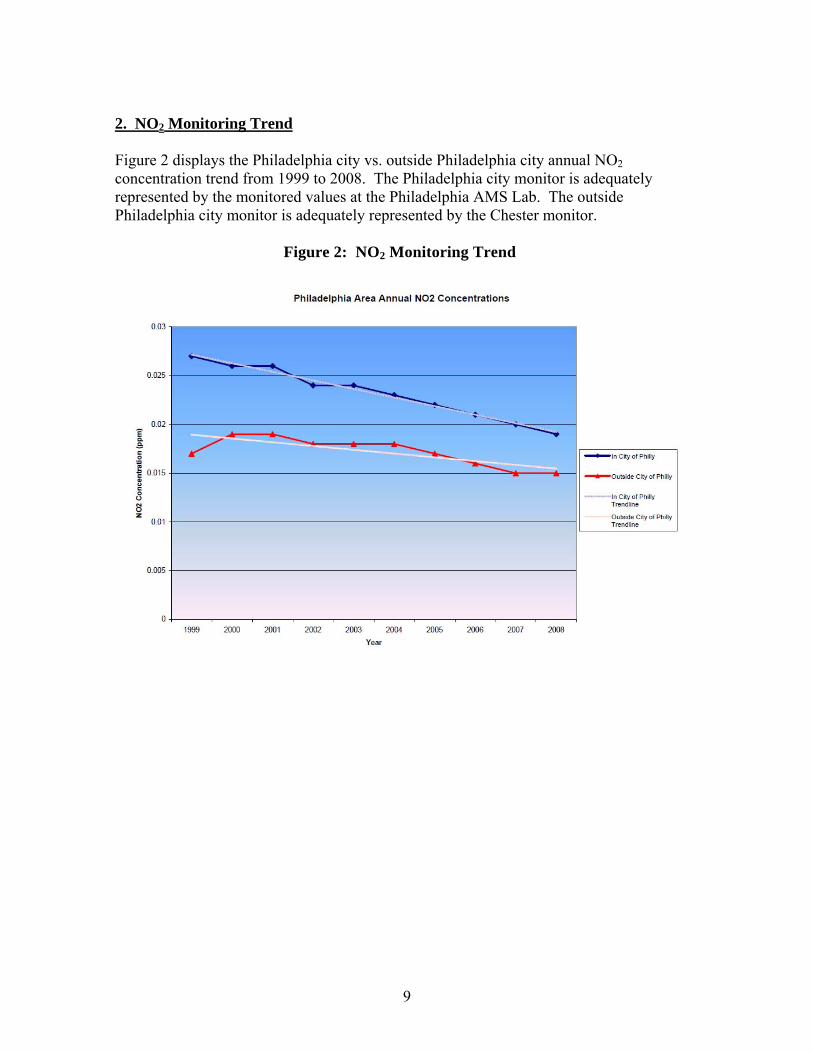
2. NO2 Monitoring Trend Figure 2 displays the Philadelphia city vs. outside Philadelphia city annual NO2 concentration trend from 1999 to 2008. The Philadelphia city monitor is adequately represented by the monitored values at the Philadelphia AMS Lab. The outside Philadelphia city monitor is adequately represented by the Chester monitor.

Figure 2: NO2 Monitoring Trend

10

3. SO2 Monitoring Trend Figure 3 displays the Philadelphia city vs. outside Philadelphia city annual SO2 concentration trend from 1999 to 2008. The Philadelphia city monitor is adequately represented by the monitored values at the Philadelphia AMS Lab. The outside Philadelphia city monitor is adequately represented by the Chester monitor.

Figure 3: SO2 Monitoring Trend

C. Seasonal Variability 1. FRM Monitoring Trends Summary of seasonal variability in FRM data: There appears to be little variability in quarterly FRM values at monitors located in the Philadelphia Area. Throughout the region, the monitors’ 3rd quarter values (summer) tend to report the highest concentrations and the 4th quarter (autumn) tend to report the lowest concentrations. This seasonal variability is primarily due to the meteorological conditions that set up in those particular seasons. The 3rd quarter tends to have more stable conditions, and the 4th quarter tends to have more volatile conditions.

11

2. Speciation Monitoring Trends Summary of seasonal variability in speciated data: Raw speciation data for the Philadelphia Area indicates some seasonal variability in the primary components. Sulfates have the largest variability with 1st quarter concentrations approximately half concentrations measured in the 3rd quarter. Nitrates vary in nearly the opposite direction with 1st quarter measurements higher than 2nd, 3rd and 4th quarter measurements. Organic carbon, elemental carbon, ammonium and crustal mass do not appear to show much seasonal variability.

12

III. EMISSION INVENTORIES

Section 51.1008 of 40 CFR Part 51 requires an inventory of pollutants to meet the requirements of section 172(c)(3) of the CAA. As specified by the EPA, the pollutants inventoried by Pennsylvania include PM10, PM2.5, SO2, NOx, VOC, and NH3. In addition, projections of future emissions have been made for the milestone year 2009. Information on the manmade sources of direct PM and its potential precursors, SO2, NOx, VOC, and NH3 was compiled for:

“Stationary sources” (or “point” sources), which are sources for which the Department collects individual emissions-related information. Generally, they represent major stationary sources but may be smaller.

“Area sources,” which are industrial, commercial, and residential sources too small

or too numerous to be handled individually. These include but are not limited to commercial and residential open burning, architectural and industrial maintenance coatings application and clean-up, consumer product use, and vehicle refueling at service stations. Where there is overlap between stationary point sources and stationary area sources, the area source values are adjusted to remove any double counting.

“Highway vehicles,” which include passenger cars and light-duty trucks, other

trucks, buses and motorcycles.

“Nonroad sources,” which encompass a diverse collection of engines, including but not limited to outdoor power equipment, recreational vehicles, farm and construction machinery, lawn and garden equipment, industrial equipment, recreational marine vessels, commercial marine vessels, locomotives, ships, and aircraft.

The inventory for the Pennsylvania portion of the Philadelphia Area was compiled for Bucks, Chester, Delaware, Montgomery and Philadelphia counties. A. Summary of 2002 Emissions An emission inventory is an estimate of the emissions from sources in a particular area. The Department developed an emission inventory for 2002, which is the base year for attainment planning purposes with respect to 8-hour ozone and PM2.5 SIPs, and for planning purposes with respect to the regional haze SIPs. The 2002 base year inventory includes the pollutants PM10, PM2.5, SO2, NOx, VOC, and NH3. The inventory consists of sources in four sectors: stationary point sources, stationary area sources, highway vehicle sources and nonroad sources. MANE-VU compiled a regional inventory from the emission inventories of the Northeastern and Mid-Atlantic states. This regional inventory was used to perform the regional modeling analysis used in Pennsylvania’s air quality

13

management planning efforts to attain the 8-hour ozone NAAQS and the PM2.5 NAAQS, and to prepare the regional haze plan. An emissions inventory for the base year, 2002, was developed in accordance with EPA guidance4. Table III-1 summarizes the emissions for 2002.

Table III-1: 2002 Annual Emissions (Tons per Year)

Philadelphia Area 2002 PM2.5 PM10 SO2 NOx VOC NH3

Stationary Point Sources 2139 3430 23745 22124 8183 256

Area Sources 10020 55224 13153 13029 59227 4821

Highway Vehicle Sources 1033 1492 1920 63476 33974 2614

Non-Road Sources 1535 1611 1640 21619 21589 14

Totals 14727 61758 40459 120248 122973 7705 B. Summary of Inventory Methodologies Inventory development methodology is summarized below. Stationary Point Sources. The Department requires owners and operators of larger facilities to submit annual production figures and emission calculations each year. Throughput data are multiplied by emission factors from Factor Information Retrieval (FIRE) Data System and the EPA’s publication series AP-42 and are based on Source Classification Codes (SCC). Each process has at least one SCC assigned to it. If the owners and operators of facilities provide more accurate emission data based upon other factors, these more accurate emission estimates supersede those calculated using SCC codes. Appendix B-1 includes information on stationary point source emission methodology, and Appendix B-2 is the data set for facility 2002 annual emissions. Appendix B-3 is a table documenting the banked emissions reduction credits for the five-county Philadelphia area in the 2009 emission projection. Area Sources. Area source emissions are generally estimated by multiplying an emission factor by some known indicator or collective activity for each area source category at the county level. Pennsylvania estimates emissions from area sources using emission factors and SCC codes in a method similar to that used for Stationary Point Sources. Emission factors may also be derived from research and guidance documents if those documents are more accurate than FIRE and AP-42 factors. Throughput estimates are derived from county-level activity data, by apportioning national or statewide activity data to counties, from census numbers, and from county employee numbers. County employee numbers are based upon North American Industry Classification System (NAICS) codes to establish

4 Emissions Inventory Guidance for Implementation of Ozone and Particulate Matter National Ambient Air Quality Standards (NAAQS) and Regional Haze Regulations – EPA-454/R-05-001. August, 2005. Updated November, 2005.

14

that those numbers are specific to the industry covered. More specific information on the procedure used for each industry type is contained in Pennsylvania 2002 Area Source Criteria Air Pollutant Emission Estimation Methods, (E.H. Pechan & Associates, Inc., February 2004) which is contained in Appendix C-1. Appendix C-2 is a table containing stationary area sources emissions data for the five-county Philadelphia area. Highway Vehicle Sources. The Department employs an emissions estimation methodology that uses the current EPA-approved highway vehicle emission model, MOBILE 6.2, to estimate highway vehicle emissions. In addition, Pennsylvania uses a MOBILE pre- and post-processing software package called PPSUITE to process and compile Pennsylvania’s robust highway network and detailed highway vehicle data. The Pennsylvania Department of Transportation (PennDOT) provided estimates of vehicle miles traveled (VMT) by vehicle type and roadway type. The Pennsylvania methodology is consistent with the January 2002 guidance published by the EPA’s Office of Transportation and Air Quality (OTAQ) entitled, Technical Guidance on the Use of MOBILE6 for Emissions Inventory Preparation. More information on highway emission methodology is available in Appendix E. Appendix E-1 provides the 2002 base year and 2009 projections of mobile (highway) VMT and annual PM2.5 direct and precursor emissions. The document summarizes the methodology and data inputs used to produce the mobile emissions inventory. Appendix E-2 is the table of 2009 five-county Philadelphia area Annual Highway Emissions listed by SCC. Appendix E-3 describes the inputs to MOBILE6.2 used to generate emission factors for a specific area. Some examples of the inputs described in Appendix E-3 are the type and frequency of vehicle emission testing, the fuel types required in the area, temperatures by month, and fleet age. The summary in Appendix E-3 indicates when default information contained in the model is used rather than specific area information. Finally, Appendix E-4 is an electronic file that provides all of the input coding for a sample segment and scenario used in Pennsylvania’s MOBILE6.2 modeling system. Nonroad Sources. The 2002 emissions for the majority of nonroad emission source categories and pollutants were estimated using the EPA NONROAD 2005 model. The NONROAD model estimates emissions for diesel, gasoline, liquefied petroleum gasoline, and compressed natural gas-fueled nonroad equipment types and includes growth factors. The National Mobile Inventory Model (NMIM) was used to estimate emissions of ammonia from sources contained in the NONROAD model. The NONROAD model does not estimate emissions from aircraft, locomotives or commercial marine vessels. Emissions from aircraft, locomotives, and commercial marine vessels were estimated using EPA guidance and best available information. If specific local operational data was available, that data was used to estimate emissions. State and national data was used if local data was unavailable. The Department has worked with the staff of the Philadelphia Division of Aviation to obtain accurate operational information for emission sources at Philadelphia International Airport (PHL). The Division of Aviation operates PHL as well as the Northeast Philadelphia Airport. The 2002 PHL Inventory described in Appendix F-3 includes

15

aircraft and aircraft-related equipment from the EPA-approved model, Emissions and Dispersion Modeling System (EDMS), and also additional on-airport highway, stationary and area source emissions. In some cases, emissions occurring at PHL are accounted for only in the regional inventory; these emissions are identified as such in the Appendix. For 2002 aircraft emissions from the Northeast Philadelphia Airport, the Department estimated emissions using operations data obtained from the Federal Aviation Administration’s (FAA) Terminal Area forecast and modeling the emissions directly with the EDMS. Emissions produced by aircraft at small airports in the Philadelphia area were estimated by using airport operation statistics, which can be found at www.airnav.com and the FAA’s Terminal Area Forecast Detailed Report. An emissions factor for a typical general aviation single engine, multi-engine, and jet engine aircraft were derived by averaging the emissions factors from a basket of emission factors for common aircraft of each of the three types of aircraft. Emission factors and operational characteristics contained in EDMS were used. The proportion of operations among the three groups of aircraft was determined by examining the number of each aircraft type based at each airport. For military operations at small airports, the type of aircraft and its emission factors are sometimes identifiable. If not, emission factors calculated to represent an “average” military aircraft are used. Growth was estimated using estimates of future operations at Philadelphia airports found in the FAA Terminal Area Forecast Detailed Report. For 2002 locomotive emissions, the Department projected emissions from a 1999 survey when the Department obtained fuel use statistics from class II and III railroads. For class I railroads, which produce most of the locomotive emissions in the Commonwealth, the Department conducted a 2002 inventory because the 1999 fuel use data for class I railroads was skewed by gridlock caused by the acquisition of Conrail by CSX and Norfolk Southern. Emissions were generated using EPA emission factors. Emissions were grown using national railroad fuel use trends supplied by the Association of American Railroads. The Philadelphia Area contains the Port of Philadelphia. The port is home to several refineries where large oil tankers often call and shipping terminals. All air emissions from commercial marine vessel (CMV) traffic in the Port of Philadelphia were estimated using the methodology outlined in the EPA’s publication Commercial Marine Activity for Deep Sea Ports in the United States, Final Report. A comprehensive understanding of the methodology can be achieved by reviewing this document. Additional understanding of the port’s operations was obtained from conversations with tugboat operators in the port and ship traffic data provided by the Philadelphia Regional Port Authority. Emission estimates were based on port activity data provided by the United States Army Corps of Engineers Waterborne Commerce Statistics Center and best available EPA nonroad emissions factors. Fuel use and emissions factors for CMV were based on the most current data available. Appendix F-1 is the technical document providing the methodology and description of the procedures used to generate 2002 and 2009 county-level pollutant emission estimates for

16

nonroad mobile engines included in the EPA’s NONROAD2005 model, locomotive engines, and aircraft operations. The table of the specific emissions data used to calculate the nonroad emissions sorted by source category is available as Appendix F-2. C. Projected Inventories 1. Summary of 2009 Estimated Emissions Table III-2 summarizes the emissions expected in 2009. These emissions take activity and emissions growth and/or controls from 2002 into account. Appendix D, relating to emissions projections, contains the technical support documents that describe the methodologies used to project the 2002 baseline emissions to 2009.

Table III-2: 2009 Projected Emissions (Tons per Year)

Philadelphia Area 2009 PM2.5 PM10 SO2 NOx VOC NH3

Stationary Point Sources 2817 3849 12658 22252 7881 357

Area Sources 10324 59533 13972 13775 55868 5749

Highway Vehicle Sources 699 1193 327 36318 20298 3118

Non-Road Sources 1356 1428 800 18874 15971 16

PHL Capacity Enhancement Program 0 0 0 0 254 0

Emission Reduction Credits Banked 23 32 442 432 1561 0

Totals 15219 66035 28200 91651 101834 9239 Sulfur and nitrogen are major contributors to the Philadelphia Area’s PM2.5 nonattainment problem. Therefore, even though the direct PM2.5 emissions increase in 2009, the reductions of PM2.5 precursors, SO2 and NOx, will ensure that the Philadelphia Area attains the PM2.5 NAAQS by 2010. 2. Growth Projection Methodologies This section describes the data, methods, and assumptions utilized in developing estimates of emissions changes between 2002 and the milestone year 2009. Appendix D-1 contains the technical support document entitled, Development of Emission Projections for 2009, 2012, and 2018 for Non-EGU Point, Area, and Nonroad Sources in the MANE-VU Region, developed by Mid-Atlantic Regional Air Management Association (MARAMA). The document provides details on the specific factors, control assumptions, and implementation schedules used in the emission projection calculations for each source category.

17

Stationary Point Sources. For electric generating units (EGUs), the Department used the EPA’s Integrated Planning Model (IPM) modeling as adjusted by the Visibility Improvement State and Tribal Association of the Southeast (VISTAS), specifically VISTAS 2.1.9, to predict the results of the EPA’s CAIR at affected facilities throughout the CAIR region. The emissions for 2009 resulting from application of the CAIR cap and trade program for annual NOx and SO2 emissions, as predicted by IPM, were used. The technical support documents that describe the methodologies used to project the emissions from EGUs, Documentation of 2018 Emissions from Electric Generating Units in the Eastern United States for MANE-VU’s Regional Haze Modeling (Alpine Geophysics, April 2008) and Future Year Electricity Generating Sector Emission Inventory Development Using the Integrated Planning Model (IPM®) in Support of Fine Particulate Mass and Visibility Modeling in the VISTAS and Midwest RPO Regions (ICF, April 2005) are included as Appendices D-2 and D-3, respectively. For non-EGU point sources, the methodology for projecting emissions to 2009 is the same as the methodology described below for stationary area sources as documented in Appendix D-1, Development of Emission Projections for 2009, 2012, and 2018 for Non-EGU Point, Area, and Nonroad Sources in the MANE-VU Region. This report was prepared for MARAMA as part of an effort to assist states in developing attainment plans for ozone and fine particles, and in developing regional haze plans. It describes the data sources, methods, and results for emission forecasts for three years, three emission sectors, two emission control scenarios, seven pollutants, and 11 states plus the District of Columbia. MARAMA developed projections for 2009, 2012, and 2018. Area Sources. Area source emissions were projected from the 2002 inventory. The factors used for the temporal allocation of projections to 2009 from the 2002 baseline inventory were provided by MARAMA, which is coordinating air quality technical projects for the Northeast and Mid-Atlantic states. The factors were in the form of Sparse Matrix Operator Kernel Emissions (SMOKE) v2.2 input files5. A table of growth factors for 2009 was provided by MARAMA. For each state, county and SCC, this table includes state growth factors derived from the Energy Information Administration (EIA) Annual Energy Outlook, 2005; and/or factors extracted from the Economic Growth Analysis System (EGAS). Where more than one factor was available, the first choice was the EIA factor followed by the EGAS factor. MARAMA also supplied tables of control factors, rule effectiveness factors, and rule penetration factors for any control measures applicable to these sources. For the area sources, these factors were available by SCC and pollutant. There may be more than one generic control factor that applies to a given SCC and pollutant. In cases

5 For additional information on the SMOKE file formats, please refer to the SMOKE v2.2 Users Manual, available from the Center for Environmental Modeling for Policy Development (CEMPD) at http://cf.unc.edu/cep/empd/products/smoke/index.cfm#Documentation.

18

where there was more than one applicable factor, the following formula may have been applied recursively to generate reductions that are a composite of those factors.

EmissionsRPRECFEmissionsEmissionsControlled

Where CF is the control factor RE is the rule effectiveness factor RP is the rule penetration factor As described for stationary point sources above, Appendix D includes the MARAMA report, Development of Emission Projections for 2009, 2012, and 2018 for NonEGU Point, Area, and Nonroad Sources in the MANE-VU Region, which documents the methodology for projecting emissions to 2009. Highway Vehicle Sources. The EPA’s approved highway vehicle emission model, MOBILE 6.2, projects highway vehicle average fleet emission factors. State specific information was used where available and appropriate. Traffic forecasts were compiled using information from PennDOT’s Traffic Information System and socioeconomic data. The Pennsylvania methodology for estimating highway vehicle emissions is consistent with the January 2002 guidance published by the EPA’s Office of Transportation and Air Quality (OTAQ) entitled, Technical Guidance on the Use of MOBILE6 for Emissions Inventory Preparation. Appendices E-1 through E-5 include specific information on the highway emissions inventory methodology, data files of emissions estimates, MOBILE6.2 input parameters, a MOBILE6.2 sample input file, and the traffic growth forecasting system report. As shown in Table III-3, VMT for the future analysis year increases 17% from 25.3 billion to 29.6 billion VMT within the five-county Philadelphia area. Despite the growth in VMT, emissions of the most significant vehicle-related precursors are significantly lower in the future analysis year.

Table III-3: Five-County Philadelphia Area VMT and Emissions

Direct PM PM Precursors

YEAR VMT PM2.5 PM10 VOC NOx SO2 NH3

2002 25,315,915,277 1,033 1,492 33,974 63,476 1,920 2,614

2009 29,561,772,617 699 1,193 20,298 36,318 327 3,118 Nonroad Sources. Projected emissions for the majority of nonroad emission source categories and pollutants were estimated using the EPA NONROAD 2005 model, which contains default assumptions for projected years. The NMIM estimated future NH3 emissions from source categories in the NONROAD model. The NONROAD model and NMIM estimate emissions for diesel, gasoline, liquefied petroleum gasoline, and compressed natural gas-fueled nonroad equipment types and include growth factors.

19

The Department worked with the staff of the Philadelphia Division of Aviation to obtain accurate operational information for emission sources at Philadelphia International Airport (PHL). Emissions from commercial aircraft are estimated using the EPA-approved Emissions & Dispersion Modeling System (EDMS). Growth was estimated using estimates of future operations at PHL from the Federal Aviation Administration’s (FAA) APO Terminal Area Forecast Detailed Report. The complete methodology for determining emissions produced from normal airport operations at PHL is described in Appendix F-3. Major construction is anticipated at PHL to relieve aircraft congestion, potentially starting in 2010. Emissions from small aircraft were calculated by using airport operation statistics, which can be found at www.airnav.com and the FAA’s APO Terminal Area Forecast Detailed Report. For locomotive emissions, the Department projected emissions from 2002 to 2009, using national fuel consumption data obtained from the Association of American Railroads and the EPA emission factors developed for the locomotive fleet in future years. Commercial marine vessel emissions were grown using projected activity, fuel use and emission estimates from the EPA document, Final Regulatory Analysis: Control of Emissions from Marine Diesel Engines, November 1999. Additional information about nonroad emission projection methodologies can also be found in Appendix F. Appendix F-1 is the technical document providing the methodology and description of the procedures used to generate 2002 and 2009 county-level pollutant emission estimates for nonroad mobile engines included in the EPA’s NONROAD2005 model, locomotive engines and aircraft operations. The table of nonroad emissions data sorted by source category is available as Appendix F-2. PHL Capacity Enhancement Program. PHL is planning to implement the Capacity Enhancement Program (CEP). The CEP will be an effort to reduce ground delays at the airport and throughout the nationwide air traffic system. The estimated maximum annual emissions of VOC, 254 tons, from the CEP were specifically identified and accounted for in the projected inventory in order to provide an emissions budget for the PHL CEP in accordance with the General Conformity Regulation in 40 CFR §93.158(a), (relating to criteria for determining conformity of general Federal actions). The methodology for estimating emissions produced during the CEP is described in Appendix F-4. The purpose of general conformity is: 1) not to cause or contribute to a new violation of the NAAQS, 2) not to increase the frequency or severity of existing violations of the NAAQS, and 3) not to delay the timely attainment of any NAAQS or any required interim emission reductions or milestones. PHL is one of the most congested airports in the nation. The CEP when complete will reduce aircraft delays and overall emissions at PHL. As of early 2010, the FAA, the agency taking the federal action, was considering two alternatives which were titled

20

Alternative A and Alternative B. Alternative A would produce fewer emissions than Alternative B. Emissions from Alternative A would be produced mostly in the first 5 years of the project while maximum emissions from Alternative B would occur at about year 10 of the project or 2020. Because the Department cannot determine which alternative will eventually be built, the maximum level of emissions produced due to aircraft delay and construction emissions from Alternative B are included as two line items in the 2009 inventory. In addition, the airport has implemented many mitigation projects that have reduced emissions from aircraft and ground support equipment operations. Mostly these emission reductions have addressed PM2.5 and NOx. Not many emission reduction projects are possible to reduce emissions of VOC on airport property. Pennsylvania proposes to establish budgets for CEP emissions of VOC in order to ensure that the CEP emissions do not impede clean air goals established in the SIP. The CEP budgeted emissions of VOC will not impede the clean air goals in the SIP because the VOC emissions used to model attainment of the fine particulate standard were over 10,000 tons in excess of the VOC emissions that were projected in the 2009 emissions inventory. Once the EPA approves the SIP, including the 2009 projected emissions inventory (Table III-2), a general conformity budget for PHL’s CEP project for VOC will be established. D. Reasonable Further Progress (RFP) Requirements Section 172(c)(2) of the CAA requires that plans for nonattainment areas provide reasonable further progress. In accordance with 40 CFR 51.1009, if a state submits an attainment demonstration for an area which demonstrates that the area will attain the PM2.5 NAAQS within five years of designation, the state is not required to submit a separate RFP plan. In that case, compliance with the emission reduction measures in the attainment demonstration and SIP will meet the requirements for achieving RFP for the area. This attainment demonstration and SIP revision demonstrate that the Philadelphia Area will attain the PM2.5 NAAQS by the area’s attainment date of April 2010, which is within five years of designation. Therefore, compliance with the emission reduction measures described in this plan meets the requirements for achieving RFP for the area. E. Motor Vehicle Emission Budgets for Transportation Conformity Section 176 of the CAA provides a mechanism by which federally funded or approved highway and transit plans, programs, and projects are determined not to produce new air quality violations, worsen existing violations, or delay timely attainment of the NAAQS. EPA regulations issued to implement transportation conformity provide that motor vehicle emission “budgets” establish caps of these emissions that cannot be exceeded by the predicted transportation system emissions in the future. Transportation agencies in Pennsylvania are responsible for making timely transportation conformity determinations. The responsible agency in the five-county Philadelphia area is the Delaware Regional Planning Commission, the designated Metropolitan Planning Organization (MPO) under federal transportation planning requirements.

21

Pennsylvania proposes to establish budgets for highway emissions for direct PM2.5 and NOx in order to ensure that transportation emissions do not impede clean air goals in the next decade and beyond. The information in Table III-5, once the EPA approves it for purposes of conformity, will establish transportation conformity budgets for the five-county Philadelphia area. Amendments to the 40 CFR part 93 transportation conformity regulations to address the 1997 PM2.5 standard were published in the Federal Register on May 6, 2005 (70 FR 24280) to account for PM2.5 and its precursors. Section 93.102 requires conformity determinations to be applicable to direct emissions of PM2.5 and NOx (unless a determination is made that transportation-related emissions are not significant contributors to PM2.5), but to emissions of SO2, VOC, and NH3 only if a finding is made that transportation-related emissions of these pollutants are significant contributors to PM2.5. Motor vehicle emissions of SO2, VOC, and NH3 were analyzed to determine if motor vehicle budgets should be established for these pollutants. Table III-4 illustrates the on-road mobile source fraction of the total 2009 inventory for each of these pollutants. Motor vehicle emissions of VOC and NH3 account for 20% and 34% of the total projected 2009 inventory for VOC and NH3, respectively. Motor vehicle emissions of SO2 account for 1% of the total projected 2009 inventory for SO2.

Table III-4 Comparison of 2009 On-Road Mobile Precursor Emissions to the Total

Projected 2009 Inventory

2009 SO2 VOC NH3

On-Road Mobile Source Projected Inventory (Tons) 327 20298 3118

Total Projected 2009 Inventory (Tons) 28200 101834 9239

Percent of Total Projected 2009 Inventory (%) 1.16 19.93 33.75 Motor vehicle emissions budget for SO2, VOC, and NH3 are needed only if the state air agency director or the EPA Regional Administrator makes a finding that motor vehicle emissions budgets must be established in order to attain the NAAQS for PM2.5. Because the reactions that form particulate matter from emissions of VOC are complex and highly variable, there is considerable uncertainty regarding the contribution of VOC to particulate formation. Likewise, much uncertainty remains regarding the role of NH3 in particulate formation. As discussed earlier in Section I, the Commonwealth is not considering VOC or NH3 as PM2.5 precursors for the purpose of the attainment plan because of the uncertainty surrounding their role in particulate formation. Therefore, this SIP revision is not establishing a motor vehicle emission budget for VOC or NH3. As shown in Table III-4, motor vehicle emissions of SO2 are a small percentage of the total inventory. Based on these facts and the fact that no applicable finding has been made for these pollutants, this SIP revision is only establishing motor vehicle emission budgets for direct PM2.5 and NOx, as shown in Table III-5.

22

Table III-5: Motor Vehicle Emission Budgets

2009 PM2.5 NOx Tons/year 699 36318

The Department has included direct PM2.5 re-entrained road dust emissions from paved and unpaved roads in the area source inventory. However, a number of fugitive dust studies have indicated that the PM2.5 / PM10 ratios measured by EPA FRM samplers are significantly lower than predicted by AP-42 emission factors. As a result, the PM2.5 emission estimates using AP-42 are biased high by as much as a factor of two, compared to FRM samplers. The Department believes that the emissions from paved and unpaved roads are significantly over-predicted and, therefore, has not included those emissions in the motor vehicle emission budgets at this time. Appendix C-2, relating to area source annual emissions, contains estimates of the PM2.5 emissions attributable to paved and unpaved roads. Transportation construction-related fugitive dust emissions are not a significant contributor to the air quality problem. At the Philadelphia Area speciation monitor, the crustal component was found to be small compared to other components of PM2.5 (see Section V, Figure 5). Given that construction-related fugitive dust is one of many source categories contributing to the crustal material observed at the monitor, and transportation construction is a small subset of all construction, it is safe to conclude that transportation construction-related fugitive emissions are insignificant.

23

IV. CONTROL STRATEGIES

A. Permanent and Enforceable Control Measures This section describes the federal and state measures that will provide the direct PM2.5, SO2 and NOx emission reductions leading to emission reductions and attainment of the standard. A summary of the quantity of emission reductions expected from 2002 to 2009 is included in Table IV-1. (Positive values indicate emission reductions, negative values indicate an increase in emissions.) The emission reduction estimates account for any anticipated growth in the activity of sources regulated by the strategy. For some pollutants and categories, emissions in 2009 are anticipated to be higher than they were in 2002. In those cases, projected growth in emissions is larger than anticipated emission reductions from control measures for that pollutant and source category. Each measure is explained in greater detail in the following sections.

Table IV-1: Summary of Emission Reductions 2002-2009 from Control Measures

2002-2009 Difference PM2.5 SO2 NOx Stationary Point Sources -678 11087 -128 Area Sources -304 -819 -745 Highway Vehicle Sources 334 1593 27158 Nonroad Sources 179 841 2745 Total -469 12702 29030

Note: Positive values indicate emission reductions. Negative values indicate an increase in emissions. 1. Stationary Point Sources Clean Air Interstate Rule (CAIR). EPA’s CAIR (70 FR 25162, May 12, 2005) was remanded to EPA for revisions by the United States Court of Appeals for the District of Columbia on December 23, 2008. The Court ordered the EPA to fix the flaws in CAIR, but did not set a deadline. EPA intends to promulgate a replacement rule in 2011. In the meantime, CAIR is being implemented. Pennsylvania transitioned from the NOx SIP Call to the federal CAIR in 2009. The CAIR is to provide the incentive for large electric generation units (EGUs) to reduce emissions below 2002 levels throughout the 28-state CAIR region. Pennsylvania and other nearby states were required to adopt a regulation implementing the requirements of the CAIR or an equivalent program. On April 28, 2006, the EPA promulgated Federal Implementation Plans (FIPs) to reduce the interstate transport of NOx and SO2 that contribute significantly to nonattainment and interfere with maintenance of the 8-hour ozone and PM2.5 NAAQS. The EGUs in Pennsylvania were regulated under the FIP until the EPA approved a SIP revision for the implementation of

24

CAIR for the affected EGUs, at which point the approved CAIR SIP revision superseded the FIP requirements in Pennsylvania. The Pennsylvania CAIR regulation was published in the Pennsylvania Bulletin on April 12, 2008. (38 Pa.B. 1705) On May 23, 2008, the Department submitted to the EPA a SIP revision for the Department’s CAIR regulatory requirements under §§ 145.201-145.223 (relating to CAIR NOx and SO2 trading programs), effective April 12, 2008 (38 Pa.B. 1705), that provide for a CAIR NOx Ozone Season Trading Program and a CAIR NOx Annual Trading Program. The EPA approved the Department’s CAIR regulation as a SIP revision effective December 10, 2009 (74 FR 65446). Interstate Pollution Transport Reduction -- In response to the federal NOx SIP call rule, Pennsylvania and other covered states adopted NOx control regulations for large industrial boilers and internal combustion engines, EGUs, and cement plants. The regulation covering industrial boilers and electric generators required emission reductions to commence May 1, 2003, while the regulation covering large internal combustion engines and cement plants required emission reductions to commence May 1, 2005. The EPA approved these regulations, found in 25 Pa. Code Chapter 145, on August 21, 2001 (66 FR 43795) and September 29, 2006 (71 FR 57428). Small Sources of NOx, Cement Kilns, and Large Stationary Internal Combustion Engines. The Department established additional ozone season requirements for small sources of NOx in the counties of Bucks, Chester, Delaware, Montgomery, and Philadelphia in regulations that were adopted December 11, 2004. The rules (25 Pa. Code Chapter 129) apply to owners and operators of certain boilers, turbines, and stationary internal combustion units located in Bucks, Chester, Delaware, Montgomery, and Philadelphia Counties. The emission limits are differentiated by fuel type and allow alternative compliance mechanisms. By November 1st of each year, owners and operators of these sources must surrender NOx allowances if actual emissions exceed allowable emissions. The amendments required the NOx emission limits to be implemented by May 1, 2005. EPA approved this program on September 29, 2006 (71 FR 57428). New Source Review Programs. The federal New Source Review (NSR) programs are preconstruction review and permitting programs applicable to new or modified major stationary sources subject to Title I, Parts C and D of the federal CAA. The programs consist of the Prevention of Significant Deterioration (PSD) requirements, which are applicable in areas attaining the NAAQS, and the Nonattainment NSR requirements, which are applicable in geographic areas not attaining and maintaining the NAAQS. The Department’s PSD regulations, codified in 25 Pa.Code Chapter 127, Subchapter D, were approved by the EPA on August 21, 1984 and codified at 40 CFR § 52.2058 (49 FR 33128). The federal PSD regulations codified in 40 CFR Part 52 are incorporated by reference in their entirety in 25 Pa. Code § 127.83 (relating to adoption by reference). The PSD program requires any new source to implement Best Available Control Technology (BACT) and limits a new source's allowable impact on the environment.

25

The EPA granted “limited” approval of the Department’s revised NSR regulations codified in 25 Pa.Code Chapter 127, Subchapter E, and published a final rule on December 7, 1997 (62 FR 64722). On October 19, 2001, the EPA converted the limited approval to a “full” approval for all areas of the Commonwealth except the five-county Philadelphia area (Bucks, Chester, Delaware, Montgomery, and Philadelphia counties) (66 FR 53904). Nonattainment NSR requirements include compliance with the lowest achievable emission rate and emission offsets.

These federally enforceable programs, incorporated in the Commonwealth’s SIP, will also reduce emissions to provide continued improvements. Federal Standards for Hazardous Air Pollutants. Federal standards to control hazardous air pollutants (HAPs) require Maximum Achievable Control Technology (MACT) at units located at major sources of HAPs. The EPA has issued a series of regulations that are applicable to sources in Pennsylvania. These MACT standards are adopted and incorporated by reference in Section 6.6 of Pennsylvania’s Air Pollution Control Act and implementing regulations and are also included in federally enforceable permits issued by the Department for affected sources. Controls with a 2002 compliance date and earlier are included in the base year inventory for 2002, while controls with a compliance date of 2003 and later are included in the projection inventories. A list of the categories for which federal MACT standards have been issued is contained in Appendix D-1. Source Surveillance. Pursuant to 40 CFR Part 51, Subpart K (relating to source surveillance), the SIP revision is required to provide for monitoring of the status of compliance with any rules and regulations that set forth any portion of the control strategy. These include provisions, as applicable, for:

emissions reports and recordkeeping for stationary sources; periodic testing and inspection of stationary sources; enforcement and complaint investigation of visible emission limitations; enforceable test methods for emission limits; and continuous emission monitoring for stationary sources.

Subpart K also requires monitoring of the implementation of transportation control measures (TCMs). There are no TCMs in this SIP. After review, the Department finds that the rules and regulations for stationary sources, which are part of the control strategy for attaining the PM2.5 standard, as well as the Department’s comprehensive permitting program requirements in 25 Pa. Code Chapter 127 and the Commonwealth’s SIP in 40 CFR 52.2020, meet the requirements of Subpart K.

26

2. Highway Vehicle Sources Even with increases in VMT that occur from 2002 through 2009, highway vehicle emissions will continue to decrease. As more vehicles subject to cleaner new car standards replace older vehicles subject to less stringent new vehicle standards, the fleet as a whole emits fewer emissions, compensating for the increase in vehicle miles traveled. These decreases can be attributed to the programs described below. Federal Motor Vehicle Control Programs (FMVCP) and Pennsylvania Clean Vehicle Program for passenger vehicles and light-duty trucks and cleaner gasoline. Tier 1 tailpipe standards established by the CAA Amendments of 1990 include NOx and VOC limits for light-duty gasoline vehicles (LDGVs) and light-duty gasoline trucks (LDGTs). These standards began to be phased in 1994. Evaporative VOC emissions were reduced in gasoline-powered cars starting with Model Year (MY) 1998.

In 1998, under the authority of section 177 of the CAA, the Department adopted the Pennsylvania Clean Vehicles Program (28 Pa. B. 5873, Dec. 5, 1998). The Pennsylvania Clean Vehicles Program incorporates by reference certain California Low Emission Vehicle (CA LEV) emission standards for passenger cars and light-duty trucks. As required under Section 177 of the CAA, these provisions are identical to the low emission standards adopted by California. The regulation does not incorporate by reference the California zero emissions vehicle (ZEV) or emissions control warranty systems statement provisions.

In the same rulemaking, the Department adopted the National Low Emission Vehicle (NLEV) program as a compliance alternative to the Pennsylvania Clean Vehicles Program. The NLEV program became effective in the Ozone Transport Region (OTR) in 1999. Pennsylvania’s New Motor Vehicle Emissions Control Program regulations in 25 Pa. Code Sections 126.401-126.441 allowed automobile manufacturers to comply with NLEV instead of the CA LEV program through MY 2005. These regulations affected vehicles 6,000 pounds and less and were the regulations in effect for new motor vehicles in the baseline year, 2002.

In 1999, the EPA promulgated regulations more stringent than NLEV (Tier 2), starting with MY 2004. In order to participate in NLEV, Pennsylvania had been required to adopt language that extended its “commitment” to NLEV until MY 2006. In practical terms, the NLEV program was replaced for MY 2004 and later by the more stringent Federal “Tier 2” vehicle emissions regulations, 65 FR 6698 (Feb. 10, 2000), and vehicle manufacturers operating under the NLEV program became subject to the Tier 2 requirements.

Pennsylvania amended the former New Motor Vehicle Control Program (which included the Pennsylvania Clean Vehicles Program) in 2006. The Clean Vehicles Program continues to incorporate the California Low Emission Vehicle Program (CA LEV II) by reference. As amended, the program affects MY 2008 and newer passenger cars and light-duty trucks vehicles. 36 Pa. B. 7424 (Dec. 9, 2006).

27

Emissions for milestone years were estimated based on compliance with the Pennsylvania Clean Vehicles Program according to the methodology described in section 7.4.1 of the Technical Guidance on the Use of MOBILE6.2 for Emissions Inventory Preparation published by the EPA’s OTAQ in January 2002. This methodology is further explained in Appendix E. The Department is assuming in its MOBILE modeling that the federal Tier 2 program applies to subject vehicles sold in Pennsylvania from MY 2004 through MY 2007 and the Pennsylvania Clean Vehicles Program applies to subject vehicles sold in MY 2008 and beyond. Reformulated Gasoline. Gasoline sold in the Philadelphia Area is required by the CAA to be the cleaner-burning reformulated gasoline meeting standards established in Section 211 of the CAA. This federally-enforced program has been in place since January 1995. Heavy-Duty Diesel Control Programs. The EPA promulgated more stringent national regulations for heavy-duty engines and vehicles (over 14,000 pounds) starting with MY 2004. In addition, consent decrees with seven of the largest heavy-duty engine manufacturers required, among other terms, that diesel engines made by these companies comply with these 2004 standards two model years early, in MY 2002. Pennsylvania includes these programs as provided in the MOBILE model. In 2002, the Department adopted the Heavy-Duty Diesel Emissions Control Program for model years starting after May 2004. The program incorporates California standards by reference and requires MY 2005 and subsequent new heavy-duty diesel highway engines to be those certified by California. California standards were more stringent than federal standards for the two model years between expiration of the consent decrees discussed above and the implementation of more stringent federal standards affecting MY 2007 and beyond. However, EPA’s MOBILE model already assumes that the engines would comply with consent decree standards, even without an enforcement mechanism. The Department has used MOBILE defaults to calculate emissions from MY 2005 and 2006 highway engines. The EPA adopted new emission standards for heavy-duty engines and vehicles for MY 2007 and subsequent. For diesel engines, the standards will be phased in from 2007 to 2010 for NOx and VOCs. For gasoline engines, the standards will be phased in during MY 2008 and 2009. Federal and California standards are virtually identical for MY 2007. For MY 2008, California adopted requirements for idling restriction engine programming and an optional “clean NOx idle” standard. However, there is no EPA-approved methodology to estimate emission reductions from this requirement. Therefore, the emission estimates use assumptions of the federal rule for MY 2007 through 2010. Because the new engine standards are adversely affected by sulfur in fuel, the EPA also requires most highway diesel fuel to contain no more than 15 parts per million (ppm) of sulfur, beginning in the fall of 2006. There is a temporary compliance option allowing refiners to continue to produce up to 20 percent of their highway diesel fuel at 500 ppm

28

fuel until 2010. The Department uses MOBILE defaults to estimate the effects of the phase-in provision. Vehicle Emission Inspection/Maintenance Program. The five-county Philadelphia area has had a vehicle emissions inspection program since 1984. In early 2004, Pennsylvania revised the implementation of its Vehicle Emission Inspection/Maintenance (I/M) Program in the five-county Philadelphia area. The program applies to gasoline-powered vehicles 9,000 pounds and under, MY 1975 and newer. For vehicles MY 1996 and newer, the program consists of an annual on-board diagnostics test and a gas cap pressure test. For subject vehicles MY 1995 and older, the program consists of an annual tailpipe test, visual inspection of pollution control devices to ensure they are present, connected and the proper type for the vehicle and a gas cap pressure test. For vehicles older than 25 years, the program is a visual inspection and gas cap test. These regulations can be found in 67 Pa. Code Chapter 177. Pennsylvania submitted the revised emissions program as a SIP revision on December 1, 2003. The EPA approved the SIP revision on October 6, 2005. (70 FR 58313). Low sulfur gasoline. Simultaneously with the Tier 2 program, the EPA published a regulation requiring the reduction of sulfur in gasoline beginning in 2004, with full implementation in 2006. Sulfur levels are capped at 80 ppm per gallon and annual refinery averages must be no more than 30 ppm. The emission reduction analysis uses the default assumptions provided in MOBILE6 to account for the implementation of the federal sulfur standard rule. Diesel Vehicle Idling Restrictions. On October 9, 2008, Governor Rendell signed the Diesel-Powered Commercial Motor Vehicle Idling Act (Act 124 of 2008). Act 124 of 2008 went into effect on February 6, 2009. This Act restricts subject drivers and owners statewide from idling a diesel-powered motor vehicle engaged in commerce with a gross vehicle weight of 10,001 pounds or more for more than five minutes in any continuous 60-minute period. Also, no owner or operator of a location where the aforementioned vehicles load, unload or park may allow the vehicles to idle for more than 5 minutes in a 60-minute continuous period. Act 124 of 2008 specifically excludes some vehicles, such as motor homes and farm vehicles used in farm applications. Additional exemptions are allowed for certain vehicles being used in specific applications. Truck drivers may idle sleeper-berth equipped vehicles for the purposes of long duration travel rest if the temperature is extremely hot or cold. In May 2010, this temperature exemption expires. A properly labeled “low-NOx idle” engine may idle for an unlimited amount of time. Act 124 of 2008 will be enforced by Department personnel, and by state and local law enforcement personnel. The law preempts and supersedes local ordinances, although rules in Allegheny County and Philadelphia County that are determined by those counties to be more stringent than the law may remain in effect. The Department estimates that 50 percent of all long duration idling for Class 8 trucks will be eliminated in 2010 when the temperature exemption for vehicles with sleeper berths expires. Statewide emission reductions are estimated to be 1610 tons, 45 tons and 30 tons per year for NOx, VOC, and PM2.5, respectively. Emission reductions expected from this strategy are not included in

29

the projected emissions inventory for 2009 for two reasons: 1) the first year was a period of education to the regulated community; and 2) most of the emission reductions from the law are expected to come from long-term travel rest idling associated with sleeper berth equipped vehicles. 3. Nonroad Sources The EPA has adopted a series of regulations affecting new diesel-powered (“compression ignition”) and gasoline-powered (“spark ignition”) nonroad engines of various sizes (horsepower) and applications. Information on these federal rules, including their implementation dates, can be found at www.epa.gov/nonroad. The Department used the assumptions built into the nonroad model (NONROAD2005) to estimate emissions for all milestone years. No new national or international regulations are expected to be applicable to aircraft by the attainment date. While the EPA has published a notice of proposed rulemaking for more stringent standards for locomotives and large commercial marine diesel engines, the agency has not finalized any new standards. The EPA will also require diesel fuel used in most nonroad applications to contain less sulfur. The sulfur will prevent damage to the more advanced emission control systems needed to meet the engine standards; it will also reduce fine particulate emissions from diesel engines. In 2007, fuel sulfur levels were limited to 500 ppm for nonroad applications other than ocean-going marine vessels. In 2010, fuel sulfur levels will be reduced to the same sulfur concentration as in highway fuel, 15 ppm; this requirement applies in 2012 to locomotive and marine diesel fuel. B. Reasonably Available Control Measures/Reasonably Available Control Technology Analysis Section 172(c) of the CAA requires states to “provide for implementation of all reasonably available control measures (RACM) as expeditiously as practicable.” The regulatory requirement for RACM and reasonably available control technology (RACT) for PM2.5 SIP revisions is codified in 40 CFR 51.1010: “For each PM2.5 nonattainment area, the state shall submit with the attainment demonstration a SIP revision demonstrating that it has adopted all reasonably available control measures (including RACT for stationary sources) necessary to demonstrate attainment as expeditiously as practicable and to meet any RFP requirements.” The EPA states in the Clean Air Fine Particle Implementation Rule preamble that it encourages states to conduct multi-pollutant analyses for PM2.5 and ozone to cull out potential RACM: “They can also try to use consistent meteorological fields and emissions inventories so that the same control strategies are relatively easy to evaluate for both ozone and PM2.5.

30

Modeling the same future year(s) for PM2.5 and ozone can also make it easier to evaluate the impacts of controls on both pollutants. It should be noted that there are no specific modeling requirements other than the recommendation to try to harmonize the ozone, PM2.5, and regional haze analyses whenever possible.”6

The Commonwealth participated in two such collaborative processes with other states in the region. First, the OTC states formed a workgroup to identify and evaluate candidate control measures. Working from a preliminary list of approximately 1,000 potential control measures, the workgroup identified and analyzed 30 candidate control measures. Appendix G-1 contains the OTC report entitled, Identification and Evaluation of Candidate Control Measures, Final Technical Support Document (MACTEC, Feb. 2007). The initial list of control measures considered is available as Appendix G-2. Based on the OTC Workgroup analysis, the Commissioners recommended that States consider emission reductions from the following source categories: • Consumer Products • Portable Fuel Containers • Adhesives and Sealants Application • Diesel Engine Chip Reflash • Cutback and Emulsified Asphalt Paving • Asphalt Production Plants • Cement Kilns • Glass Furnaces • Industrial, Commercial, and Institutional (ICI) Boilers • Regional Fuels • Electric Generating Units (EGUs) The final report, included as Appendix G-1, contains more detailed information about the process and includes tables summarizing the emission reduction potential of each control measure by source category and projection year. There are five subsections discussing the control measure and emission reductions for the five source category sectors: non-EGU point sources, area sources, EGUs, onroad mobile sources, and nonroad mobile sources. The Department also participated in an assessment of control measures for pollutants and sources affecting visibility through the MANE-VU regional haze planning process. As part of this effort, MANE-VU developed a list of possible control measures for consideration. The following categories were selected for analysis:

Coal and oil-fired EGUs Point and area source industrial, commercial and institutional boilers Cement kilns Lime kilns The use of heating oil Residential wood combustion and open burning

6. 72 FR 20609.

31

Appendix G-3 contains the final report entitled, Assessment of Reasonable Progress for Regional Haze in MANE-VU Class I Areas (MACTEC, July 2007) from the MANE-VU control measure assessment project. This report presents the results of an analysis of the economic and environmental impacts of the potential control scenarios that could be implemented by MANE-VU states to reduce emissions from selected source categories in order to make reasonable progress toward meeting visibility improvement goals. As required under 40 CFR 51.1010, a SIP revision for a PM2.5 nonattainment area must demonstrate that all RACM, including RACT for stationary sources, necessary to demonstrate attainment as expeditiously as practicable have been adopted. The cumulative impact of implementing available measures must be considered in determining whether a particular emission reduction measure or set of measures is required to be adopted as RACM. Potential measures that are reasonably available considering technical and economic feasibility must be adopted as RACM if, considered collectively, they would advance the attainment date by one year or more. As discussed earlier in this document, the Philadelphia Area expects to monitor attainment at the end of 2009. Therefore, any RACM measures would need to be in effect in 2008. The Department determined that there were no additional control measures that could be adopted by January 1, 2008. In addition, existing measures and those planned for implementation by 2009 are expected to enable the Philadelphia Area to attain the 1997 PM2.5 NAAQS. Therefore, no further actions on RACM or RACT are warranted. Although the measures explored by the OTC and MANE-VU workgroups are not required as RACM, many are worthwhile measures that Pennsylvania is currently pursuing. Others are measures that Pennsylvania may consider for the future. C. Other Measures - VOC Control Measures Although VOC is not a regulated PM2.5 precursor for the Philadelphia Area, several VOC control measures are discussed in this section because they are included in the modeling associated with this attainment demonstration. Portable Fuel Containers. The Department adopted a portable fuel container regulation, 25 Pa. Code Chapter 130, Subchapter A, to address VOC loss resulting from permeation through portable gasoline containers, evaporative loss through container openings, and spillage during the filling of small tanks on machines such as lawn mowers, chain saws and jet skis. The regulation was submitted to the EPA as a SIP revision on March 26, 2003 and approved on December 8, 2004 (69 FR 70893). Consumer Products. This regulation applies statewide to any person who sells, supplies, offers for sale, or manufactures certain consumer products on or after January 1, 2005, for use in the Commonwealth. The program is contained in 25 Pa. Code Chapter 130, Subchapter B. It was submitted to the EPA as a SIP revision on March 26, 2003 and approved on December 8, 2004 (69 FR 70895). Additional regulations were adopted on October 11, 2008 and submitted to the EPA as a SIP revision on April 14, 2009.

32

Architectural and Industrial Maintenance (AIM) Coatings. The Pennsylvania AIM Coatings regulation applies statewide to any person who supplies, sells, offers for sale, or manufactures, blends or repackages an AIM coating for use within the Commonwealth, as well as a person who applies or solicits the application of an AIM coating within the Commonwealth. The AIM coating program requirements are specified in 25 Pa. Code Chapter 130, Subchapter C. The regulation was submitted to the EPA as a SIP revision on December 3, 2003, with a supplement submitted on October 19, 2004. The EPA approved the provisions as an element of the SIP on November 23, 2004 (69 FR 69080).

33

V. ATTAINMENT DEMONSTRATION AND WEIGHT OF EVIDENCE (WOE)

A. Attainment Demonstration Background and Objectives The EPA issued fine particle standards in 1997 after evaluating hundreds of health studies and conducting an extensive peer review process. The 1997 annual health-based standard for PM2.5 is 15.0 μg/m3, based on the 3-year average of annual mean PM2.5 concentrations. The EPA also established a 24-hour health-based standard of 65 μg/m3, determined by the 3-year average of the 98th percentile of 24-hour concentrations. The EPA set levels to protect the environment at the same levels as it set the health-based standards. Note that while the EPA has subsequently revised the 24-hour standard in 2006 to be more protective, EPA designated the Philadelphia Area as nonattainment because it violated the 1997 annual standard of 15.0 μg/m3 based on 2001-03 monitoring data. Therefore, this SIP revision compares air quality data to the 1997 24-hour standard (65 μg/m3). On April 1, 2003, the EPA issued a memorandum, “Designations for the Fine Particle National Ambient Air Quality Standards” outlining the schedule for designating areas under the PM2.5 standard and related guidance on nine factors to consider in identifying nonattainment areas. The CAA provides for states and tribes to submit designation recommendations to the EPA, and it requires the EPA to provide time for consultation in cases where the Administrator plans to promulgate a designation that modifies the state or tribal recommendation. On December 17, 2004, the EPA published its air quality designations and classifications for the 1997 PM2.5 NAAQS. These designations became effective on April 5, 2005. Figure 4 graphically depicts all of the PM2.5 nonattainment areas in Pennsylvania. Based on 2006 – 2008 monitoring data, all monitors in the Philadelphia Area meet the EPA’s annual PM2.5 standard (15.0 μg/m3). The Philadelphia Area’s maximum 2008 annual design value of 14.5 μg/m3 was observed at the Broad Street monitor. Based on 2006 – 2008 monitoring data, all monitors within the Philadelphia Area are monitoring attainment of the 1997 24-hour PM2.5 standard (65 μg/m3). The maximum 2008 24-hour design value in the Philadelphia Area was 36 μg/m3, observed at the New Garden monitor. The Philadelphia Area is required to attain the PM2.5 standard no later than five years from the effective date of designation of April 5, 2005 (April, 2010). The purpose of the attainment demonstration is to ensure, through grid modeling, that projected emissions (with controls) will not cause the nonattainment area to exceed the 1997 PM2.5 NAAQS. A complex grid model was run and processed over the entire Northeast to determine if the Philadelphia Area would attain the PM2.5 standard by April 5, 2010. The procedures followed in this modeling analysis are in accordance with EPA’s Guidance on the Use of Models and Other Analyses for Demonstrating Attainment of Air Quality Goals for Ozone, PM2.5, and Regional Haze (EPA-454/B-07-002, April 2007). A brief summary of the modeling analysis used in this demonstration is included in the following

34

sections. The Department submitted a modeling protocol to the EPA in May 2006 for the Philadelphia Area that includes a more thorough description of the modeling analysis.

Figure 4: Pennsylvania’s PM2.5 Nonattainment Areas

B. Philadelphia Area Conceptual Model Description This section provides a brief description of the conceptual model for the Philadelphia Area. The conceptual model was based on information from the Northeast States for Coordinated Air-Use Management (NESCAUM) final report entitled The Nature of the Fine Particle and Regional Haze Air Quality Problems in the MANE-VU Region: A Conceptual Description (2006) and the Department’s modeling protocol documentation (October 2007).

35

Fine particulate formation in the eastern United States is a complex process involving local and regional meteorology, topography, chemistry and transport. Since a violation of an annual standard potentially involves a large range of conditions throughout the year, it is difficult to determine a direct cause-and-effect relationship for such a violation. Violations of the annual standard ensure a large range of conditions will contribute to nonattainment making direct cause-and-effect relationships difficult to determine. In general, the following statements can be used to provide a working conceptual model that describes the annual PM2.5 nonattainment problem in the Philadelphia Area:

Secondary fine particulate formation is a major contributor to annual PM2.5

nonattainment in the Philadelphia Area. Sulfates, organic carbon and nitrates make up almost 75% of the annual fine-particulate concentrations (see Figure 5).

Fine-particulate chemistry favors sulfate formation during the warm summer months and nitrate formation during the colder winter months.

In the summer time, large high pressure systems create favorable conditions for the oxidation of SO2, which eventually forms sulfates. These sulfates then contribute to episodes of high particulate concentrations.

In the winter time, local temperature inversions concentrate emissions near the surface leading to periods of elevated fine-particulate concentrations. This is especially apparent if significant terrain features are present.

Continuous measurements in the Philadelphia Area correlate well with the FRM data. This indicates measurements from the continuous monitor generally reflect actual concentrations in the nonattainment area.

Average concentrations from the continuous monitor show a general diurnal pattern with higher concentrations in the overnight and early morning hours than during the day, due to atmospheric conditions and possibly local mobile source emissions (peaks during rush hour traffic, etc.)

In addition to the diurnal signal noted in the continuous monitoring data, there is a strong weekly pattern in the continuous monitoring data with higher PM2.5 concentrations on weekdays than on weekends.

A range of control measures will be necessary to attain the PM2.5 standard in the Philadelphia Area due to the complex interaction between local and regional emissions and local meteorological conditions. Sulfates and nitrates are formed primarily through atmospheric reactions of precursor emissions of SO2, NOx and NH3. Organic carbon is a combination of secondary organic particles formed from emissions of VOC and the organic portion of primary PM2.5 that is directly emitted or condenses near its source. Currently, our understanding of sulfate and nitrate chemistry and its impacts on PM2.5 concentrations far exceeds our understanding of contributions from anthropogenic VOCs. This is important because sulfates, nitrates and organic carbon are major contributors to the fine particulate problem in the Philadelphia Area. Therefore, it is reasonable to assume that a mixture of regional and local SO2 and NOx controls in addition to VOC controls implemented for attainment of the 8-hour ozone standard will assist in attaining the PM2.5

standard.

36

Figure 5: Philadelphia Area Percentage of Total Mass Based on Speciated PM2.5 Data Collected at Chester

Averaged 2005 to 2007 Monitored Values

C. Modeling Domain and Photochemical Modeling System The modeling demonstration for the Philadelphia Area relies heavily on the OTC SIP quality-modeling platform. Ozone modeling was the primary focus of this effort. OTC’s interaction with MANE-VU and NESCAUM allowed it, through the regional modeling centers, to do additional year-round modeling for PM2.5 and Regional Haze. EPA’s Guidance on the Use of Models and Other Analyses for Demonstrating Attainment of Air Quality Goals for Ozone, PM2.5, and Regional Haze (EPA-454/B-07-002, April 2007) does not recommend a particular model or models for use in a SIP attainment demonstration. The OTC modeling committee used the CMAQ photochemical grid model (version 4.5) as part of its SIP modeling platform (OTC Final Modeling Protocol, 2006). CMAQ is an Eulerian grid model capable of simulating air pollutant concentrations in the atmosphere using mathematical equations to characterize chemical and physical properties. Meteorological and emission input files must be prepared regardless of which photochemical grid model is used. The regional fine particulate modeling analysis encompassed an entire year of simulation for the year 2002. This approach provided a good variety of episodes to characterize the Philadelphia Area’s PM2.5 nonattainment problem.

37

Figure 6 shows the modeling domain used by the OTC Modeling Workgroup. A nested-grid approach was used with the lower resolution outer grid providing boundary conditions for a more refined grid covering the area of interest. The modeling domain was chosen to be large enough to properly simulate regional transport. The outer domain boundary is far enough from the inner grid’s boundary so that clean-boundary condition assumptions along the outer domain’s boundary are realistic and probably do not unduly influence concentrations within the inner domain.

Figure 6. OTC Modeling Study Domain

Outer grid at 36-kilometer resolution, inner grid at 12-kilometer resolution The meteorological files used in CMAQ were produced using the Pennsylvania State University/National Center for Atmospheric Research (PSU/NCAR) Mesoscale Model version 5 (MM5). MM5 is a limited-area, nonhydrostatic, terrain-following sigma-coordinate model designed to simulate or predict mesoscale atmospheric circulation. The model is publicly available and has been used for various air quality modeling studies in the past. The OTC Modeling Committee also examined two emissions processors (EMS2001 and SMOKE, both using CB4 chemistry) in its prior work and concluded that there are differences between them that could be minimized by forcing the models to use a common speciation and surrogate database. For areas with an attainment date of no later than April 5, 2010 for the PM2.5 NAAQS, the emission reductions need to be implemented no later than the beginning of 2009. A determination of attainment will be based on air quality monitoring data collected in 2007, 2008, and 2009. Therefore, the year to project future emissions should be no later than the last year of the three-year monitoring period, which in this case is 2009.

38

The emissions inventory was developed for 2009 using standard emissions projection techniques. The 2009 inventories developed by MANE-VU were used in the attainment demonstration. The most recently available inventories from other regional planning organizations (RPOs) in the modeling domain were also used. Emission inventory guidance documents were followed for developing projection year inventories for point, area, mobile, and biogenic emissions. These procedures address projections of spatial, temporal, and chemical composition change between the base year and projection year. The control strategies developed for evaluation in the attainment demonstration were selected by the OTC’s Control Strategy Committee. These were selected from groups of strategies developed by the technical subcommittees responsible for identifying and developing the regulations and/or other control measures. Consideration was given to maintaining consistency with control measures likely to be implemented by other modeling domains that may be involved in region-wide analysis. Also, technology-based emission reduction requirements mandated by the CAA are included in the future year model runs. D. Model Performance Evaluation A critical component of every air quality modeling study is the model performance evaluation where modeled estimates for the current year base case are compared against observed values to assess the model’s accuracy and provide an indication of its reliability. The results presented here serve as an illustration of some of the model evaluation and assessment, as outlined in the EPA modeling guidance document entitled, Guidance on the Use of Models and Other Analyses for Demonstrating Attainment of Air Quality Goals for Ozone, PM2.5, and Regional Haze (EPA-454/B-07-002, April 2007), performed on the Base Year 2002 CMAQ simulation. The New York State Department of Environmental Conservation (DEC), Division of Air Resources, conducted a performance evaluation of the 2002 base case CMAQ simulation on behalf of the OTC member states. Model performance was evaluated over the entire year, except for the July 6-9, 2002 period which was excluded from this analysis since the observed PM2.5 and organic mass (OM) data at many sites were greatly affected by Canadian forest fires. Appendix H, relating to Modeling Demonstration, provides comprehensive operational and diagnostic evaluation results. Highlights of this evaluation are provided in the following sections. The analysis examines model performance over a wide area, including the entire OTR plus the State of Virginia (OTR+). 1. Daily PM2.5 Mass Model performance over the entire OTR+ region was examined using several statistics. These included overall mean fractionalized bias (MFB) and mean fractional error (MFE).

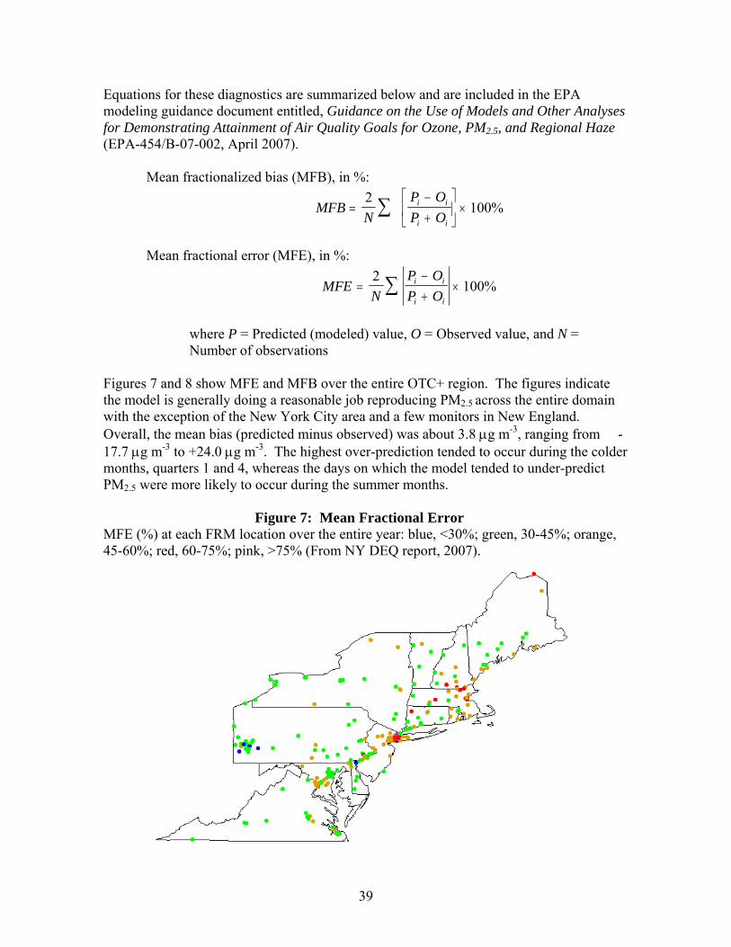
39

Equations for these diagnostics are summarized below and are included in the EPA modeling guidance document entitled, Guidance on the Use of Models and Other Analyses for Demonstrating Attainment of Air Quality Goals for Ozone, PM2.5, and Regional Haze (EPA-454/B-07-002, April 2007).

Mean fractionalized bias (MFB), in %:

MFBN

P O

P Oi i

i i

2

100%

Mean fractional error (MFE), in %:

MFEN

P O

P Oi i

i i

2100%

where P = Predicted (modeled) value, O = Observed value, and N = Number of observations

Figures 7 and 8 show MFE and MFB over the entire OTC+ region. The figures indicate the model is generally doing a reasonable job reproducing PM2.5 across the entire domain with the exception of the New York City area and a few monitors in New England. Overall, the mean bias (predicted minus observed) was about 3.8 g m-3, ranging from -17.7 g m-3 to +24.0 g m-3. The highest over-prediction tended to occur during the colder months, quarters 1 and 4, whereas the days on which the model tended to under-predict PM2.5 were more likely to occur during the summer months.

Figure 7: Mean Fractional Error MFE (%) at each FRM location over the entire year: blue, <30%; green, 30-45%; orange, 45-60%; red, 60-75%; pink, >75% (From NY DEQ report, 2007).

40

Figure 8: Mean Fractional Bias MFB (%) at each FRM location over the entire year: gray, <-45%; blue, -45 to -15%; green, -15 to 15%; orange, 15-45%; red, 45-75%; pink, >75% (From NY DEQ report, 2007).

2. PM2.5 Speciation PM2.5 is composed of several components. The primary components noted in the monitoring data include sulfates, nitrates and organic carbon; other components do not significantly contribute to PM2.5 concentrations. For proper performance, CMAQ predictions for each individual component of PM2.5 must also be examined. Data from the various speciation networks in the OTR+ region were compared to model predicted values for the base case (2002). Again, data from the July 6-9, 2002 period was excluded from this analysis due to the Canadian forest fires. Sulfates (SO4

-) are one of the primary contributors to the Philadelphia Area’s PM2.5 nonattainment. Figure 11 depicts modeled and actual sulfate measurements in the OTR+ region. The CMAQ model appears to reproduce actual sulfate concentrations quite well along with its seasonal variability. Nitrates (NO3

-) are another important contributor to the Philadelphia Area’s PM2.5 nonattainment. CMAQ does less well reproducing actual concentrations than it does for sulfates. Modeled concentrations appear to be less accurate during the colder months (1st and 4th quarters) than the warmer months.

41

OM is another important contributor to the Philadelphia Area’s PM2.5 nonattainment. CMAQ does not do well reproducing the seasonal variability of OM though it does appear to do a better job reproducing observed winter values.

Figure 9: Time Series of SO4 Mass Time series of SO4 mass based on the composite average of all 21 Interagency Monitoring of Protected Visual Environments (IMPROVE) monitors across the OTR+ region. IMPROVE is a long-term monitoring program established in the mid-1980s to provide data needed to assess the impacts of new emission sources, identify existing man-made visibility impairment, and assess progress toward improving visibility in National Parks and Wilderness Areas. The observed values are denoted with the black diamonds, the model predictions are denoted with gray squares (From NY DEQ report, 2007).

0

2

4

6

8

10

12

14

16

18

SO

4 (

g m

-3)

OBS PRED

NY DEQ’s model performance included an analysis of the meteorological model used to drive CMAQ, as well as actual PM2.5 values and PM2.5’s speciated components. Appendix H-2 is a technical listing of the model inputs, as well as an assessment of the MM5 simulation to real-world data. The analysis shows that, in general, the performance of the MM5 is reasonable both at the surface and in the vertical, thereby providing confidence in the use of these data in the CMAQ simulations. Both the MM5 and CMAQ runs appear to meet performance criteria over the entire OTR+ domain. Therefore, it can be assumed the modeling platform provides meaningful information in regard to projected 2009 PM2.5 concentrations that will be used to assess the Philadelphia Area’s future attainment of the PM2.5 standard.

42

E. Projected 2009 Design Values for the Philadelphia Nonattainment Area 1. Overview As mentioned previously, the Philadelphia Area has an attainment date of April 5, 2010. The PM2.5 NAAQS include an annual standard of 15.0 μg/m3 based on the 3-year average of annual mean PM2.5 concentrations, and a 24-hour standard of 65 μg/m3 based on the 3-year average of the 98th percentile of 24-hour concentrations. This section summarizes the procedures that are used to demonstrate attainment of the PM2.5 NAAQS. As described in EPA’s Guidance on the Use of Models and Other Analyses for Demonstrating Attainment of Air Quality Goals for Ozone, PM2.5, and Regional Haze (EPA-454/B-07-002, April 2007), an attainment demonstration consists of (a) analyses that estimate whether selected emissions reductions will result in ambient concentrations that meet the NAAQS, and (b) an identified set of control measures that will result in the required emissions reductions. The necessary emission reductions for both of these attainment demonstration components may be determined by relying on results obtained with air quality models. EPA’s Guidance on the Use of Models and Other Analyses for Demonstrating Attainment of Air Quality Goals for Ozone, PM2.5, and Regional Haze (EPA-454/B-07-002, April 2007) recommends applying a modeled attainment test to the air quality modeling results to determine if the PM2.5 NAAQS will be met. Additional technical or corroboratory analyses may also be used as part of a “supplemental analysis” or a more stringent “weight of evidence” determination to supplement the modeled attainment test and to further support a demonstration of attainment of the NAAQS. The modeled attainment test and additional corroborative analyses are described in further detail in the remaining portions of this section. 2. Modeled Attainment Test The purpose of a modeling assessment is to determine if control strategies currently being implemented “on the books” (OTB) and proposed control strategies (“on the way” or OTW) will lead to attainment of the NAAQS for PM2.5 by the attainment year of 2009. The modeling is applied in a relative sense, similar to the 8-hour ozone attainment test: however, the PM2.5 attainment test is more complicated and reflects the fact that PM2.5 is a combination of many different species. In the test, ambient PM2.5 is divided into major components. Then, a relative response factor (RRF) and future design value (DVF) is calculated for each of the PM2.5 components. Since the attainment test is calculated on a per species basis, the attainment test for PM2.5 is referred to as the Speciated Modeled Attainment Test (SMAT). The following sections outline the process to determine that 2009 projections of PM2.5 will meet the NAAQS from regional modeling, as suggested in EPA’s modeling guidance.

43

3. Determine Baseline Design Values The first step in any attainment test process is to determine the baseline design value (DVB). The EPA guidance recommends using a DVB that is the average of the three design value periods that straddle the baseline inventory year (i.e., the average of the 2000-2002, 2001-2003, and 2002-2004 design value periods for a 2002 baseline inventory year). This results in a 5-year weighted average, with the baseline year having the heaviest weight (i.e., {[2000] + 2*[2001] + 3*[2002] + 2*[2003] + [2004]}/9). For the SMAT process, a mean PM2.5 DVB is determined, as well as component specific DVB, for each quarter. The following section will detail the calculation of baseline design values needed for the PM2.5 attainment test. Mean PM2.5 Baseline Design Values To begin the SMAT process, a mean PM2.5 DVB is calculated on a quarterly basis for each FRM monitor in the PM2.5 nonattainment areas. Concentrations are calculated based on calendar quarters (Q1: January - March; Q2: April - June; etc.) as the NAAQS is calculated for a calendar year, and the quarters need to fit evenly within a year. Calculating the attainment test on a quarterly basis also allows states to examine the differences in PM2.5

composition that occur during the different seasons. Speciated Baseline Conditions The monitored attainment test for PM2.5 utilizes both PM2.5 and individual PM2.5 component species. A separate RRF is calculated for each PM2.5 species. In order to perform the recommended modeled attainment test, states should divide observed mass concentrations of PM2.5 into seven components (plus passive mass):

1. Mass associated with sulfates (SO4) 2. Mass associated with nitrates (NO3) 3. Mass associated with ammonium (NH4) 4. Mass associated with organic carbon (OC) 5. Mass associated with elemental carbon (EC) 6. Mass associated with particle bound water (PBW) 7. Mass associated with “other” primary inorganic particulate matter (Crustal) 8. Passively collected mass or the mass of the blank filter (Passive)

This yields the following formula in order to calculate PM2.5:

PM2.5FRM = [SO4] + [NO3] + [OC] + [EC] + [NH4] + [PBW] + [Crustal] + [Passive] The second part of the process is to use the quarterly mean PM2.5 DVBs with speciated data to calculate the quarterly mean concentrations of these 7 components at the FRM sites. This need to speciate the FRM data presents two issues:

44

1. FRM measurements and speciated PM2.5 measurements do not always measure the same mass.

2. Not all FRM monitoring sites have co-located Speciation Trends Network (STN) speciation monitors.

The following sections will explain how these issues are addressed to produce the speciated values needed for this attainment demonstration. SANDWICH As the EPA’s Guidance on the Use of Models and Other Analyses for Demonstrating Attainment of Air Quality Goals for Ozone, PM2.5, and Regional Haze (EPA-454/B-07-002, April 2007) notes, recent data analyses have noted that the FRM monitors do not measure the same components and do not retain all of the PM2.5 that is measured by STN samplers. Therefore, measurements from FRM monitors cannot be directly compared to speciation measurements from the STN monitors. By design, the FRM mass measurement does not retain all ammonium nitrate and other semi-volatile materials (negative sampling artifacts) and includes particle bound water associated with sulfates, nitrates and other hygroscopic species (positive sampling artifacts). This results in concentrations (and percent contributions to PM2.5 mass) that may be different from the ambient levels of some PM2.5 chemical constituents. To resolve the differences between FRM and STN total mass, EPA recommends using the “sulfate, adjusted nitrate, derived water, inferred carbonaceous” (SANDWICH) material balance approach. With the SANDWICH approach, nitrate mass is adjusted to account for volatilization based on hourly meteorology parameters. Subsequently, quarterly average nitrate, sulfate, elemental carbon, ammonium and crustal mass can be calculated, as well as the Degree of Neutralization (DON) of sulfates. Next, the mass of particle bound water can be calculated from the previously obtained DON, sulfate, nitrate, and ammonium values. (See more details on particle bound water calculations in the Annual SMAT Results section, below). Finally, organic carbon is calculated by taking the difference between the total PM2.5 mass as measured at the FRM monitor, and the calculated component mass (i.e., OC from mass balance ([OCMmb] = PM2.5FRM - {[EC] + [SO4] + [NO3] + [NH4] + [PBW] + [Crustal] + [Passive]}), where the Passive (mass) is the FRM sampling artifact normally set equal to 0.5). EPA Region 3 office provided SANDWICHed data for the Philadelphia Area monitors. For a description and use of the SANDWICH method, see the Definition of SANDWICHed STN Data (EPA, 2006). Speciated Profiles While the SANDWICH method reconciles the differences between FRM and STN, a lingering issue is that not all FRM monitoring sites have co-located STN monitors to provide speciated data. EPA guidance suggests four measures that can be taken to resolve the lack of speciated data:

45

1. Use of concurrent data from a nearby speciated monitor 2. Use of representative data (from a different time period) 3. Use of interpolation techniques to create a spatial field using ambient speciation

data 4. Use of interpolation techniques to create spatial fields, and gridded modeling

outputs to adjust the species concentrations Of the four methodologies, EPA recommends using one of the spatial interpolation techniques to estimate species concentrations at FRM sites that do not have speciation data (numbers 3 and 4, above). To assist in this task, EPA began developing a software tool called “Modeled Attainment Test Software” (or MATS) that would perform the spatial analysis of described options number 3 and 4. However, the MATS tool was not available at the time this analysis was completed. In trying to pursue the EPA recommended course of action, option 1 (use of concurrent data from a nearby speciated monitor) was utilized. 4. Relative Response Factor Calculations The calculation of RRFs for this study was performed using the EPA recommended method for “nearby” grid cells for a 12-kilometer horizontal grid resolution, with a 3x3 grid cell array for 12-km resolution modeling. The relative response factor used in the modeled attainment test is computed by taking the ratio of the mean of the predictions in the future to the mean predictions with baseline emissions, over all relevant days. For the 24-hour and annual PM2.5 NAAQS, the spatially averaged value of the nearby predictions (mean value of the grid cell array) was used. Each component-specific RRF was used in the modeled attainment test by taking the ratio of the mean of the spatially averaged daily predictions in the future to the mean of the spatially averaged daily predictions with current emissions. The basis for this approach is as follows:

1. Consequence of a control strategy may be “migration” of a predicted peak. If a state were to confine its attention only to the cell containing a monitor, it might underestimate the RRF (i.e., overestimate the effects of a control strategy).

2. Uncertainty in the formulation of the model and the model inputs is consistent with recognizing some leeway in the precision of the predicted location of concentrations.

3. Standard practice in defining a gridded modeling domain is to start in the southwest corner of the domain and determine grid cell location from there. Considering several cells “near” a monitor rather than the single cell containing the monitor diminishes the likelihood of inappropriate results that may occur from the geometry of the superimposed grid system.

4. The area does not exhibit strong spatial concentration gradients of observed primary PM2.5.

46

5. Annual SMAT Results A difficulty presented in estimating the future design values was missing STN data for 2000 and 2001at the Philadelphia Area monitors. This limitation restricted the calculation of SANDWICH data to the period 2002–2004. Therefore, the 2009 projected design values are based on speciation profiles developed using 2002-2004 STN data. There are four FRM monitors in the Pennsylvania portion of the Philadelphia Area that are co-located with a speciated sampler: Chester, New Garden, Elmwood, and Philadelphia AMS Lab. However, since there are eight FRM monitors within the Philadelphia Area, the Department was able to determine that the four speciated monitors (including an additional monitor in Camden, NJ) in the nonattainment area were representative of all FRM monitor locations in order to complete the SMAT analysis. RRFs were only calculated for the sulfates, nitrates, organic carbon, elemental carbon and crustal component of PM2.5. Referencing the PM2.5 FRM formula in section 3 above, the only components of PM2.5 that were not included in the RRF calculation were ammonium and water. Base and future case ammonium was calculated based on the DON value and the following formula presented in EPA’s Guidance on the Use of Models and Other Analyses for Demonstrating Attainment of Air Quality Goals for Ozone, PM2.5, and Regional Haze:

NH4 = 0.29 * NO3 + DON * SO4. The particle bound water was then calculated using the particle bound water formula estimated from the Aerosol Inorganic Model. Due to the hygroscopic nature of ammonium sulfate and ammonium nitrate, retained sulfate, nitrate and ammonium will all contain water. Therefore, the final polynomial equation (seen below and referenced (EPA, 2006 (2))) contains sulfates, nitrates and ammonium within its calculation. The equation utilized was that for low acidity.

PBW = [202049.0 – 391494.6 * S – 390912.1 * N + 442.4 * (S^1.5) – 155.3 * (N^1.5) - 293406.8 * (A^1.5) + 189277.5 * (S^2) + 377992.6 * N * S + 188636.8 * (N^2)

– 447.1 * (S^2.5) – 507.2 * (S^1.5) * N – 12.8 * (S^3) + 146.2 * (N^1.5) * S + 217.2 * (N^2.5) + 30.0 * (N^1.5) * (S^1.5) – 18.6 * (N^3) + 216267.0 * (A^1.5) * S

+ 215419.9 * (A^1.5) * N – 621.8 * (A^1.5) * (S^1.5) + 239.1 * (A^1.5) * (N^1.5) + 35413.1 * (A^3)] * (SO4 + NO3+ NH4)

where S = SO4 / (SO4 + NO3 + NH4) N = NO3 / (SO4 + NO3 + NH4) A = NH4 / (SO4 + NO3 + NH4)

Table V-1 displays the calculated quarterly RRFs for the design monitor of the Philadelphia Area, Broad Street. Based on the results of the RRF calculations, all PM2.5

constituents either remain the same or undergo a downward trend, except for the crustal portion.

47

Table V-1: Annual PM2.5 Quarterly RRF Values

Table V-2 presents the results of the annual SMAT results for all of the monitors in the Pennsylvania portion of the Philadelphia Area. The SMAT results demonstrate that the projected average annual arithmetic mean PM2.5 concentration calculated at each FRM monitor attains the annual PM2.5 NAAQS. Specifically, all DVF calculations are less than 15.0 μg/m3. Table V-2 presents the results of the annual SMAT results for a suite of regional modeling runs conducted by OTC, with each modeling run representing OTB/OTW control measures. All runs demonstrate timely attainment of the annual NAAQS.

Table V-2: Annual SMAT Results for the Philadelphia Area 2009 On The Books/On

The Way Control Measures

Source: 2000-2004 DVB quarterly concentrations calculated from data in Appendix A-2.

Quarter Sulfates Nitrates OC EC Crustal

1st 0.9429 0.8976 0.9514 0.8171 1.0988

2nd 0.7272 0.7450 0.9867 0.8083 1.1700

3rd 0.6619 0.8218 0.9875 0.7927 1.1869

4th 0.9043 0.9008 0.9848 0.8058 1.1433

2000-2004 DVB 2009 AIRS ID

Site Name County State Q1 Q2 Q3 Q4 DVF

420170012 Bristol Bucks PA 14.14 13.69 14.73 13.85 12.1

420290100 New Garden Chester PA 14.39 14.73 16.36 13.76 12.4

420450002 Chester Delaware PA 15.07 15.96 16.34 13.74 13.3

420910013 Norristown Montgomery PA 12.68 13.62 13.96 12.34 11.3

421010004 AMS Lab Philadelphia PA 15.99 14.01 15.95 13.82 12.9

421010024 NE Airport Philadelphia PA 13.58 13.63 14.95 12.96 11.9

421010047 Broad Street Philadelphia PA 16.59 16.45 15.80 15.37 13.5

421010136 Elmwood Philadelphia PA 15.70 14.20 15.27 12.99 12.7

100031003 Bellefonte New Castle DE 14.87 15.16 15.50 13.13 12.6

100031007 Lums Pond New Castle DE 13.16 14.37 16.05 10.66 11.3

100031012 Newark New Castle DE 15.27 14.91 16.53 13.14 12.6

100032004 MLK New Castle DE 16.41 15.40 17.61 14.04 13.3

340070003 Camden Camden NJ 13.99 14.54 15.76 12.47 12.3

340071007 Pennsauken Camden NJ 13.99 14.00 14.75 13.59 12.3

340155001 Gibbstown Gloucester NJ 13.92 13.43 15.08 11.39 11.7

48

6. 24-Hour SMAT Results As with obtaining the annual SMAT Results, a difficulty presented in estimating the future design values was missing STN data for 2000 and 2001 at all of the Philadelphia area monitors. This limitation restricted the calculation of SANDWICH data to the period 2002–2004. Therefore, the 2009 projected design values are based on speciation profiles developed using 2002-2004 STN data. The RRF calculations were very similar to those that were computed in the annual SMAT analysis, except that all modeled RRFs were compared with each monitoring year’s 24-hour 98th percentile design value. A quarterly analysis was completed consistent with the procedure outlined in EPA’s Guidance on the Use of Models and Other Analyses for Demonstrating Attainment of Air Quality Goals for Ozone, PM2.5, and Regional Haze (EPA-454/B-07-002, April 2007). The procedure that was completed was as follows. The top 25% of the days of the speciation and the modeling data were computed on a quarterly basis. The speciation data was compared with the quarterly PM2.5 FRM data to compute a speciated composition of the FRM data. After the RRFs were calculated (the RRF values for Elmwood, are shown below in Table V-3), these RRF values were applied to the speciated composition data to compute a 2009 speciated composition data. Once this was completed, a future year design value was reconstructed.

Table V-3: 24-hour PM2.5 Quarterly RRF Values

Quarter Sulfates Nitrates OC EC Crustal

1st 0.9549 0.9235 0.9211 0.8157 1.0852

2nd 0.6761 0.7858 0.9841 0.8091 1.1758

3rd 0.6023 0.8698 0.9947 0.7978 1.2134

4th 0.9036 0.9237 0.9830 0.8089 1.1514 Table V-4 displays the 24-hour PM2.5 SMAT results for all of the monitors within the Philadelphia Area. The SMAT results demonstrate that the projected 24-hour 98th percentile PM2.5 concentration calculated at the FRM monitor attains the 24-hour PM2.5 NAAQS. Specifically, all DVF calculations are less than 65 μg/m3. Table V-4 presents the results of the 24-hour SMAT results for a suite of regional modeling runs conducted by OTC each representing OTB/OTW control measures. All runs demonstrate attainment of the 24-hour PM2.5 NAAQS.

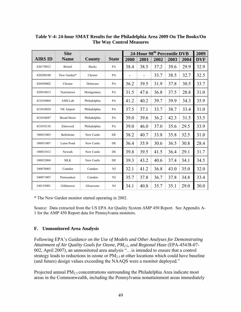
49

Table V-4: 24-hour SMAT Results for the Philadelphia Area 2009 On The Books/On

The Way Control Measures

24-Hour 98th Percentile DVB 2009AIRS ID

Site Name County State 2000 2001 2002 2003 2004 DVF

420170012 Bristol Bucks PA 38.4 38.5 37.2 39.6 29.9 32.9

420290100 New Garden* Chester PA - - 33.7 38.5 32.7 32.5

420450002 Chester Delaware PA 36.2 39.5 31.9 37.8 30.5 33.7

420910013 Norristown Montgomery PA 31.5 47.6 36.8 37.5 28.8 31.0

421010004 AMS Lab Philadelphia PA 41.2 40.2 39.7 39.9 34.3 35.9

421010024 NE Airport Philadelphia PA 37.5 37.1 33.7 38.7 33.4 31.0

421010047 Broad Street Philadelphia PA 39.0 39.6 36.2 42.3 31.5 33.5

421010136 Elmwood Philadelphia PA 39.0 46.0 37.0 35.6 29.5 33.9

100031003 Bellefonte New Castle DE 38.2 40.7 33.8 35.8 32.5 31.0

100031007 Lums Pond New Castle DE 36.4 35.9 30.6 36.5 30.8 28.4

100031012 Newark New Castle DE 39.8 39.5 41.5 36.4 29.1 31.7

100032004 MLK New Castle DE 39.3 43.2 40.6 37.4 34.1 34.5

340070003 Camden Camden NJ 32.1 41.2 36.8 43.0 35.0 32.0

340071007 Pennsauken Camden NJ 35.7 37.8 36.7 37.8 34.8 33.4

340155001 Gibbstown Gloucester NJ 34.1 40.8 35.7 35.1 29.0 30.0

* The New Garden monitor started operating in 2002. Source: Data extracted from the US EPA Air Quality System AMP 450 Report. See Appendix A-1 for the AMP 450 Report data for Pennsylvania monitors. F. Unmonitored Area Analysis Following EPA’s Guidance on the Use of Models and Other Analyses for Demonstrating Attainment of Air Quality Goals for Ozone, PM2.5, and Regional Haze (EPA-454/B-07-002, April 2007), an unmonitored area analysis “…is intended to ensure that a control strategy leads to reductions in ozone or PM2.5 at other locations which could have baseline (and future) design values exceeding the NAAQS were a monitor deployed.”

Projected annual PM2.5 concentrations surrounding the Philadelphia Area indicate most areas in the Commonwealth, including the Pennsylvania nonattainment areas immediately

50

surrounding the Philadelphia Area, are projected to attain the standard by 2009. This indicates there should be no areas where concentrations could reasonably be expected to exceed the annual PM2.5 NAAQS within the nonattainment area.

The Air Quality Modeling Group (EPA Research Triangle Park) has developed the MATS, described on p. 39, above. MATS is a PC-based software tool that can perform the modeled attainment tests for PM2.5 and ozone (O3), and perform the uniform rate of progress analysis for regional haze (visibility). However, when this analysis was conducted, MATS was still in development and therefore was not utilized within this analysis.

G. Local Area Analysis EPA’s Guidance on the Use of Models and Other Analyses for Demonstrating Attainment of Air Quality Goals for Ozone, PM2.5, and Regional Haze (2007) suggests that it may be necessary to evaluate the impact of local primary PM sources for contributions to both the 24-hour and annual NAAQS. Evaluation of local PM sources and their effects on monitor concentrations could be evaluated using a near-scale model such as AERMOD or CALPUFF. Since the end of 2008, there are a total of eight (8) FRM monitors within the Philadelphia Area; four (4) FRM monitors run by the Department and four (4) FRM monitors run by the Philadelphia AMS. In addition, there are four (4) speciation monitors and at least five (5) continuous PM2.5 monitors located within the Philadelphia Area. Pennsylvania has noted local source interference at PA DEP’s Chester monitor (PA DEP, September 2004). Chester has the second highest annual PM2.5 design value (14.1 µg/m3) and the fifth highest 24-hour design value (33 µg/m3) in the Philadelphia Area in 2008. The 24-hour design value is below the (1997) 24-hour standard indicating attainment of the NAAQS even with significant local effects. A review of the Commonwealth’s, Philadelphia County’s, Delaware’s, Maryland’s and New Jersey’s 2002 emissions from the NEI database indicates eighteen (18) large sources with greater than 50 tons per year (TPY) of direct PM2.5 emissions within 50 kilometers of the Chester PM2.5 monitor. These sources are listed in Table V-5. Each source’s PM2.5 emissions, distance from the Chester monitor, direction from the Chester monitor, county, state, and emission to distance ratio (Q/d) are included in the table.

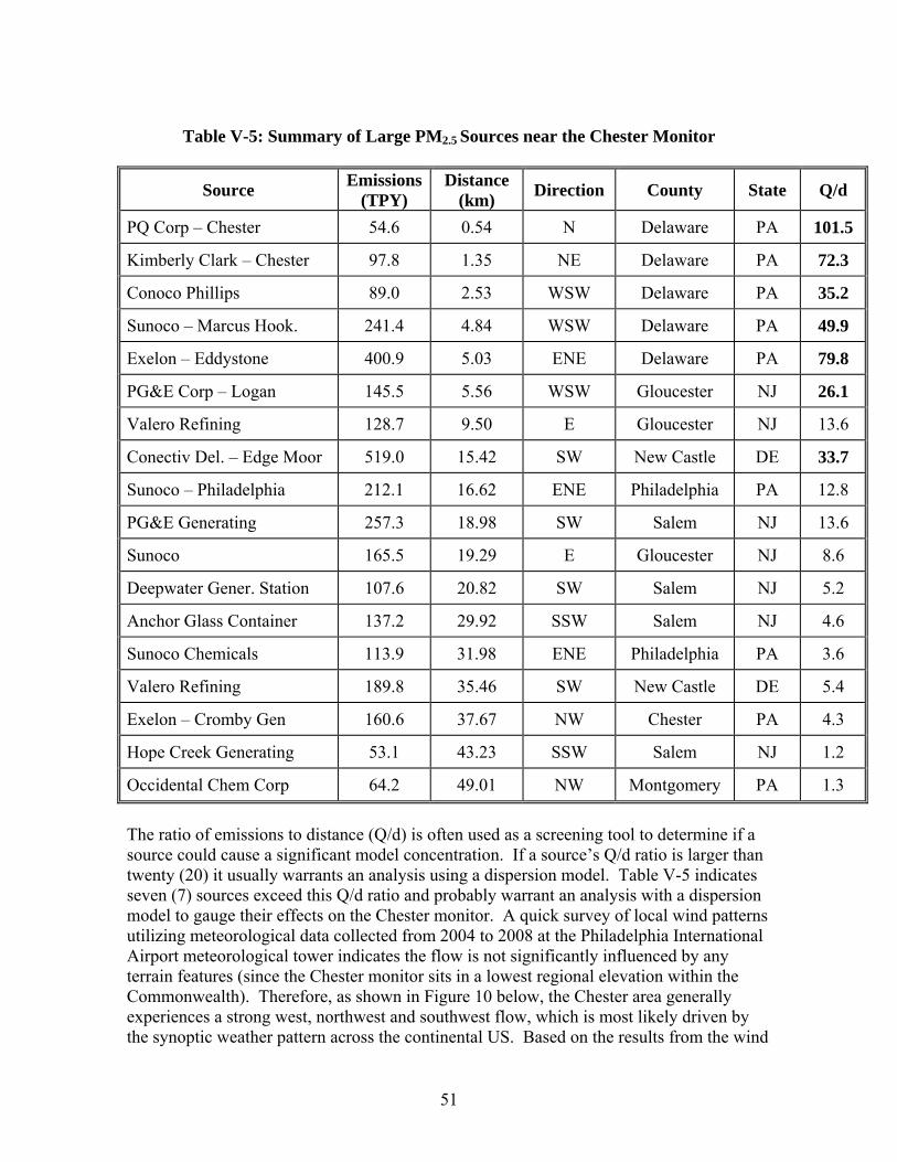
51

Table V-5: Summary of Large PM2.5 Sources near the Chester Monitor

Source Emissions

(TPY) Distance

(km) Direction County State Q/d

PQ Corp – Chester 54.6 0.54 N Delaware PA 101.5

Kimberly Clark – Chester 97.8 1.35 NE Delaware PA 72.3

Conoco Phillips 89.0 2.53 WSW Delaware PA 35.2

Sunoco – Marcus Hook. 241.4 4.84 WSW Delaware PA 49.9

Exelon – Eddystone 400.9 5.03 ENE Delaware PA 79.8

PG&E Corp – Logan 145.5 5.56 WSW Gloucester NJ 26.1

Valero Refining 128.7 9.50 E Gloucester NJ 13.6

Conectiv Del. – Edge Moor 519.0 15.42 SW New Castle DE 33.7

Sunoco – Philadelphia 212.1 16.62 ENE Philadelphia PA 12.8

PG&E Generating 257.3 18.98 SW Salem NJ 13.6

Sunoco 165.5 19.29 E Gloucester NJ 8.6

Deepwater Gener. Station 107.6 20.82 SW Salem NJ 5.2

Anchor Glass Container 137.2 29.92 SSW Salem NJ 4.6

Sunoco Chemicals 113.9 31.98 ENE Philadelphia PA 3.6

Valero Refining 189.8 35.46 SW New Castle DE 5.4

Exelon – Cromby Gen 160.6 37.67 NW Chester PA 4.3

Hope Creek Generating 53.1 43.23 SSW Salem NJ 1.2

Occidental Chem Corp 64.2 49.01 NW Montgomery PA 1.3

The ratio of emissions to distance (Q/d) is often used as a screening tool to determine if a source could cause a significant model concentration. If a source’s Q/d ratio is larger than twenty (20) it usually warrants an analysis using a dispersion model. Table V-5 indicates seven (7) sources exceed this Q/d ratio and probably warrant an analysis with a dispersion model to gauge their effects on the Chester monitor. A quick survey of local wind patterns utilizing meteorological data collected from 2004 to 2008 at the Philadelphia International Airport meteorological tower indicates the flow is not significantly influenced by any terrain features (since the Chester monitor sits in a lowest regional elevation within the Commonwealth). Therefore, as shown in Figure 10 below, the Chester area generally experiences a strong west, northwest and southwest flow, which is most likely driven by the synoptic weather pattern across the continental US. Based on the results from the wind

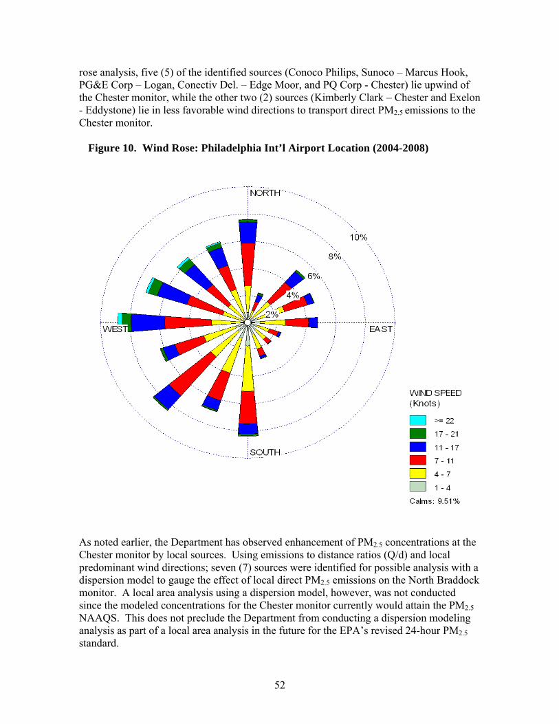
52

rose analysis, five (5) of the identified sources (Conoco Philips, Sunoco – Marcus Hook, PG&E Corp – Logan, Conectiv Del. – Edge Moor, and PQ Corp - Chester) lie upwind of the Chester monitor, while the other two (2) sources (Kimberly Clark – Chester and Exelon - Eddystone) lie in less favorable wind directions to transport direct PM2.5 emissions to the Chester monitor.

Figure 10. Wind Rose: Philadelphia Int’l Airport Location (2004-2008)

As noted earlier, the Department has observed enhancement of PM2.5 concentrations at the Chester monitor by local sources. Using emissions to distance ratios (Q/d) and local predominant wind directions; seven (7) sources were identified for possible analysis with a dispersion model to gauge the effect of local direct PM2.5 emissions on the North Braddock monitor. A local area analysis using a dispersion model, however, was not conducted since the modeled concentrations for the Chester monitor currently would attain the PM2.5 NAAQS. This does not preclude the Department from conducting a dispersion modeling analysis as part of a local area analysis in the future for the EPA’s revised 24-hour PM2.5 standard.

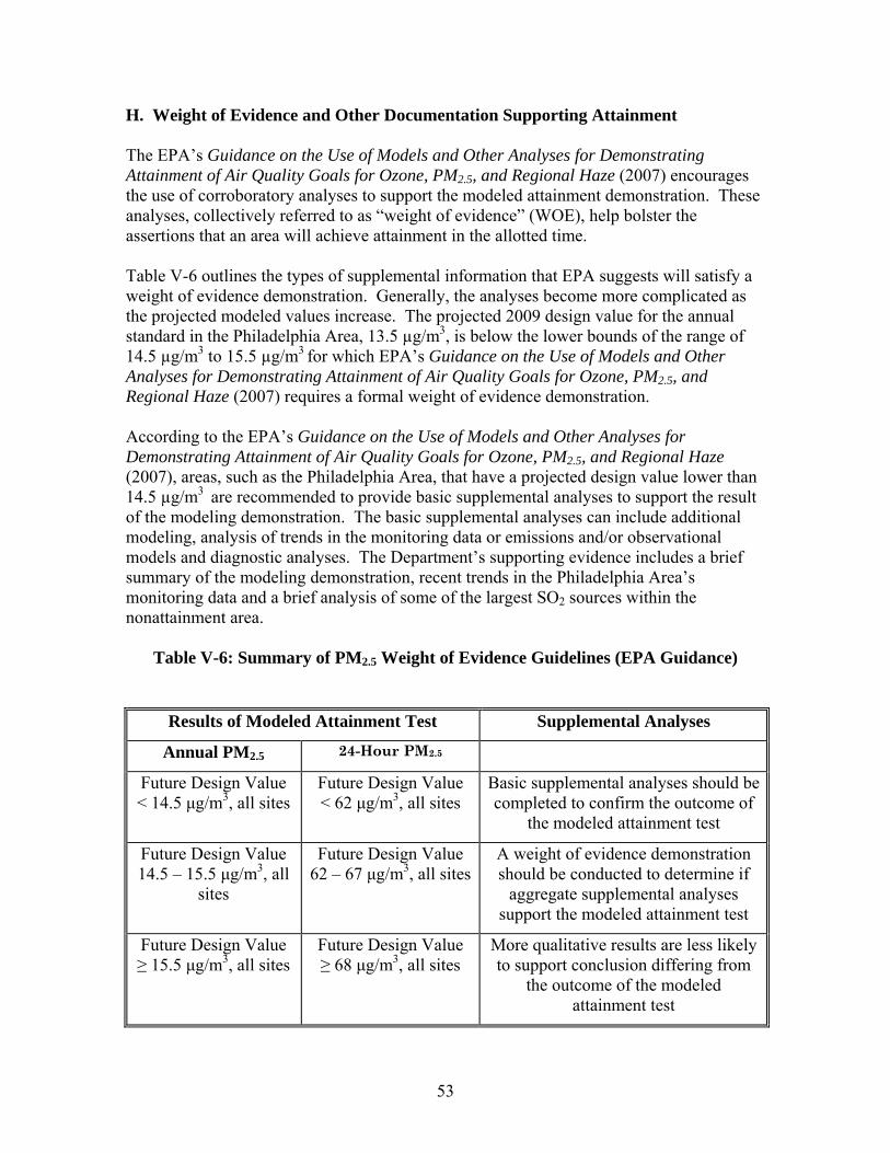
53

H. Weight of Evidence and Other Documentation Supporting Attainment The EPA’s Guidance on the Use of Models and Other Analyses for Demonstrating Attainment of Air Quality Goals for Ozone, PM2.5, and Regional Haze (2007) encourages the use of corroboratory analyses to support the modeled attainment demonstration. These analyses, collectively referred to as “weight of evidence” (WOE), help bolster the assertions that an area will achieve attainment in the allotted time. Table V-6 outlines the types of supplemental information that EPA suggests will satisfy a weight of evidence demonstration. Generally, the analyses become more complicated as the projected modeled values increase. The projected 2009 design value for the annual standard in the Philadelphia Area, 13.5 µg/m3, is below the lower bounds of the range of 14.5 µg/m3 to 15.5 µg/m3 for which EPA’s Guidance on the Use of Models and Other Analyses for Demonstrating Attainment of Air Quality Goals for Ozone, PM2.5, and Regional Haze (2007) requires a formal weight of evidence demonstration. According to the EPA’s Guidance on the Use of Models and Other Analyses for Demonstrating Attainment of Air Quality Goals for Ozone, PM2.5, and Regional Haze (2007), areas, such as the Philadelphia Area, that have a projected design value lower than 14.5 µg/m3 are recommended to provide basic supplemental analyses to support the result of the modeling demonstration. The basic supplemental analyses can include additional modeling, analysis of trends in the monitoring data or emissions and/or observational models and diagnostic analyses. The Department’s supporting evidence includes a brief summary of the modeling demonstration, recent trends in the Philadelphia Area’s monitoring data and a brief analysis of some of the largest SO2 sources within the nonattainment area.

Table V-6: Summary of PM2.5 Weight of Evidence Guidelines (EPA Guidance)

Results of Modeled Attainment Test Supplemental Analyses

Annual PM2.5 24-Hour PM2.5

Future Design Value < 14.5 μg/m3, all sites

Future Design Value < 62 μg/m3, all sites

Basic supplemental analyses should be completed to confirm the outcome of

the modeled attainment test

Future Design Value 14.5 – 15.5 μg/m3, all

sites

Future Design Value 62 – 67 μg/m3, all sites

A weight of evidence demonstration should be conducted to determine if

aggregate supplemental analyses support the modeled attainment test

Future Design Value ≥ 15.5 μg/m3, all sites

Future Design Value ≥ 68 μg/m3, all sites

More qualitative results are less likely to support conclusion differing from

the outcome of the modeled attainment test

54

2009 Projected Modeling Concentration: The Department’s attainment demonstration relies on results from the OTB/OTW CMAQ runs completed by the Virginia Department of Environmental Quality. Emissions for the base case (2002) and projected (2009) time frames were developed by MARAMA with input from all jurisdictions that are part of the OTR. Base-case and projected emissions within the Philadelphia Area appear to be reasonable; therefore, the projected design value for 2009 should reflect what will actually be monitored. Recent analyses of projected CMAQ ozone design values suggest the model may actually underestimate the impact of emission reductions on actual concentrations. This modeled underestimation of changes in ozone concentrations may be due to the model’s inability to adequately reproduce changes in ozone concentrations due to large emission reductions. If CMAQ has the same shortfall with fine particulate concentrations, then it may also overestimate the projected 2009 PM2.5 design values for the Philadelphia Area. Since the calculated design value is already well below 15.0 µg/m3, any overestimation of the projected 2009 annual PM2.5 design value provides a further cushion bolstering the argument that the Philadelphia Area will reach attainment. PM2.5 and Emission Trends: Many monitors within the region are heavily influenced by the mobile source sector. Emissions from the mobile source sector are predicted to be significantly lower in 2009 compared to 2002. As more vehicles subject to cleaner new car standards replace older vehicles subject to less stringent standards, the fleet as a whole emits fewer emissions. Figure 11 shows the annual and 24-hour PM2.5 concentrations for the Chester monitor from 1999 through 2008. Over the last two years, annual PM2.5 averages appear to have declined slightly. In fact, all PM2.5 monitors, excluding the Broad Street monitor, in the Philadelphia Area are monitoring attainment of the annual PM2.5 standard, based on 2006 – 2008 monitoring data. This may be due to a combination of weather conditions and emission decreases in the mobile source sector and may be indicative of lower future PM2.5 design values allowing the Philadelphia Area to attain the annual PM2.5 standard with a comfortable margin.

55

Figure 11: Philadelphia Area PM2.5 Trends

56

I. Conclusions

The Philadelphia Area’s projected 2009 annual PM2.5 concentration was estimated using the OTC’s modeling platform. A review of the base case (2002) run indicated the CMAQ model did a reasonable job reproducing actual concentrations. Based on this analysis, it is reasonable to assume the model can estimate the projected PM2.5 concentrations within the Philadelphia Area for 2009. The Department understands that the EPA anticipates using 2009 data to determine whether the Philadelphia Area attains the PM2.5 standard by its April 2010 attainment date.

Projected PM2.5 concentrations from CMAQ indicate the Philadelphia Area will attain the annual standard by 2009. Additional evidence supporting this conclusion includes lower concentrations at all of the PM2.5 monitors within the Philadelphia Area the last couple of years and possible model under-predictions of the air quality benefits of emission reductions.

57

VI. CONTINGENCY MEASURES FOR THE ATTAINMENT DEMONSTRATION

A. Contingency Measure Requirement Pursuant to 40 CFR 51.1012, the attainment plan for the Philadelphia Area must include a contingency plan that contains measures that qualify as contingency measures for the attainment demonstration. This section fulfills the contingency measures requirement for the attainment demonstration. The contingency plan must provide for one year of reductions needed for attainment. By 2009, emissions of SO2 and NOx in the Pennsylvania portion of the Philadelphia Area are projected to decrease by 12,259 tons and 28,597 tons, respectively. Based on modeling of the projected 2009 emissions, the Philadelphia Area is predicted to have a 2009 design value of 13.5 ug/m3. This is lower than the 15 ug/m3 required for attainment of the PM2.5 standard. Calculations were made to estimate the portion of the emission reduction that is necessary to reach the attainment concentration of 15 ug/m3 and the portion of the emission reduction that reduces the design value below 15 ug/m3 and is, therefore, excess. Table VI-1 contains information about the changes in design value and emissions expected by 2009 in the five-county Philadelphia area. Table VI-1 displays the 2002 actual and 2009 modeled design values and the 2002 actual and 2009 projected emissions of PM2.5, SO2 and NOx.

Table VI-1: Changes in Design Value and Emissions Expected by 2009

Philadelphia Area Design Value

(ug/m3) PM2.5

(tons/year)SO2

(tons/year) NOx

(tons/year)

2002 16.6 14727 40459 120248

2009 (Modeled/Projected) 13.5 15219 28200 91651

Predicted Change from 2002-2009 3.1 -492 12259 28597

As shown in Table VI-2, for each pollutant, the change in pollutant emissions was divided by the predicted change in design value to yield the design value reduction rate. Next, the change in design value necessary to attain the standard (16.6 ug/m3 – 15 ug/m3 = 1.6 ug/m3) was multiplied by the design value reduction rate to estimate the target emissions reduction. This represents the portion of emissions reduction necessary to attain the standard. The rest of the emissions reduction is beyond what is necessary for attainment and is, therefore, considered to be “excess” reduction.

58

Table VI-2: Calculation of Required and Excess Emissions Reductions

Philadelphia Area Design Value

(ug/m3) PM2.5

(tons/year) SO2

(tons/year)NOx

(tons/year)

Predicted Change from 2002-2009 3.1 -492 12259 28597

Design Value Reduction Rate (tons/ug/m3) N/A 3955 9225

Target Reductions for Attainment 1.6 N/A 6327 14760

Calculated Excess Reductions 1.5 N/A 5932 13837

The contingency requirement is calculated by dividing the target emissions reduction by seven which is the number of years between 2002 and 2009. Table VI-3 shows the calculation of the contingency requirement reduction and demonstrates that the calculated excess reduction exceeds the amount of reduction necessary for the contingency plan.

Table VI-3: Calculation of Required Contingency Plan Reductions

Philadelphia Area PM2.5 (tons/year)

SO2 (tons/year)

NOx (tons/year)

Target Reductions for Attainment N/A 6327 14760

Calculated Excess Reductions N/A 5932 13837

Contingency Requirement N/A 904 2109

Excess Reductions Satisfy Contingency Requirement

N/A Yes Yes

B. Identified Contingency Measures In addition to the calculated excess reductions shown in Tables VI-2 and VI-3 above, the Department has identified additional control measures. EPA guidance encourages early implementation of contingency measures to guard against failure either to meet a milestone or attain the standard. EPA's guidance on early implementation of control measures encourages the early implementation of required control measures and of contingency measures as a means of guarding against failures to meet a

59

milestone or to attain. The EPA states that any implemented measures (that are not needed for the rate-of-progress requirements or for the attainment requirements) would need to be “backfilled”, meaning replaced with another measure, only to the extent they are used to meet a milestone.7 The reductions from the designated contingency measures are surplus vis-à-vis the attainment demonstration contained in this SIP. As a result, the Department will not be required to replace any contingency measures that it chooses to implement in advance of the contingency plan requirement. The following describes specific control measures that are anticipated to be in place in order to bring the area back into attainment should a violation occur. On October 9, 2008, Governor Rendell signed Senate Bill 295, which became Act 124 of 2008, the Diesel-Powered Commercial Motor Vehicle Idling Act (Act 124). Act 124 went into effect on February 6, 2009. The Department estimates that 50 percent of all long duration idling for Class 8 trucks will be eliminated in 2010 when the temperature exemption for sleeper truck rest expires. Statewide emission reductions are estimated to be 1610 tons, 45 tons and 30 tons per year for NOx, VOC, and PM2.5, respectively. The Department may also utilize enhanced enforcement to obtain additional emission reductions. Significant additional reductions in NOx, direct PM2.5 and, to a limited extent, SO2 emissions will occur in emissions from highway and nonroad mobile sources after 2009. NOx emissions from mobile sources are more than one-third of the emissions in 2009. In addition, the following regulations are in development and are anticipated to be adopted in the relatively near future:

NOx controls for cement kilns NOx controls for glass furnaces Sulfur limits for fuel oil (home heating oil and residual fuel oil)

Regulations to reduce VOC emissions are also in development, including controls on the manufacture and use of adhesives, primers and sealants and regulations incorporating the Control Techniques Guidelines issued by the EPA in 2006, 2007 and 2008. Once the Department’s Bureau of Air Quality has obtained an approved request to initiate a rulemaking, the rulemaking may proceed as follows:

7 EPA, "Guidance on the Post-1996 Rate-of-Progress Plan and the Attainment Demonstration," Corrected Version as of February 18, 1994, p. 50.

60

Within 2 months: Review by Air Quality Technical Advisory Committee (AQTAC), Citizens Advisory Council and other advisory committees,8 as appropriate. Within 5 months: Environmental Quality Board (EQB) meeting/action. Within 7 months: Publication in the Pennsylvania Bulletin for comment as proposed rulemaking. Within 9 months: Public hearing takes place and comment period on proposed rule closes. Within 10 months: House and Senate Standing Committees and Independent Regulatory Review Commission (IRRC) comment on proposed rule. Within 12 months: AQTAC, Citizens Advisory Council and other committees, as appropriate, review responses to comments and draft final rulemaking. Within 15 months: EQB meeting/action. Within 16 months: IRRC action on final rulemaking. Within 17 months: Attorney General review/action. Within 18 months: Publication in the Pennsylvania Bulletin as final rulemaking and submission to the EPA as a SIP revision. The regulation would become effective

upon publication in the Pennsylvania Bulletin.

8 Other committees could include the Small Business Compliance Advisory Committee and Agriculture Advisory Committee.

61

REFERENCES SECTION I Pope III, C. Arden, M. Ezzati and D. Dockery. “Fine-Particulate Air Pollution and Life Expectancy in the United States.” New England Journal of Medicine. 360: 376-386 January 22, 2009. EPA, 2007. Clean Air Fine Particle Implementation Rule. Final Rule. 72 FR 20586 (April 25, 2007). SECTION III EPA, 2005. Emissions Inventory Guidance for Implementation of Ozone and Particulate Matter National Ambient Air Quality Standards (NAAQS) and Regional Haze Regulations. EPA-454/R-05-001. August, 2005. Updated November, 2005 Final Technical Support Document, Development of Emission Projections for 2009, 2012, and 2018 for NonEGU Point, Area, and Nonroad Sources in the MANE-VU Region. Prepared by MACTEC for MARAMA, February 28, 2007. Final Regulatory Analysis: Control of Emissions from Marine Diesel Engines, EPA, November 1999. SECTION V The Nature of the Fine Particle and Regional Haze Air Quality Problems in the MANE-VU Region: A Conceptual Description. Prepared by the Northeast States for Coordinated Air-Use Management (NESCAUM), November 2006. Summary of Pennsylvania’s PM2.5 Nonattainment Analysis, Prepared by the Pennsylvania Department of Environmental Protection, October 2007. Guidance on the Use of Models and Other Analyses for Demonstrating Attainment of Air Quality Goals for Ozone, PM2.5, and Regional Haze. EPA, EPA-454/B-07-002, April 2007. Final Air-Quality Modeling Protocol for the Annual PM2.5 NAAQS: Philadelphia-Wilmington PA-NJ-DE Annual PM2.5 Nonattainment Area, prepared by the Pennsylvania Department of Environmental Protection, October 2007. A Modeling Protocol for the OTC SIP Quality Modeling System For Assessment of the Ozone National Ambient Air Quality Standard in the Ozone Transport Region, The Modeling Committee of the Ozone Transport Commission, March 2006.

62

CMAQ Model Performance and Assessment for Base Year 2002: PM2.5 Mass and Speciation, Prepared by the New York State Department of Environmental Conservation, December 2007. Clegg, S.L., P. Brimblecombe, and A. S. Wexler, (1998), “Aerosol Inorganics Model; A Thermodynamic Model of the System H+ - NH4+ - SO42- - NO3- - H2O at Tropospheric Temperatures.”, J. Phys. Chem., 102A, 2137-2154. (http://www.aim.env.uea.ac.uk/aim/project.htm). EPA, 2004. Procedures for Estimating Future PM2.5 Values for the CAIR Final Rule by Application of the (Revised) Speciated Modeled Attainment Test (SMAT). July 26, 2004. Available on EPA’S CAIR PDF web page (www.epa.gov/CAIR/pdfs/Revised-SMAT.pdf). EPA, 2006. Definition of SANDWICHed STN Data. November 1, 2006. Available on EPA’s Air Explorer web page (www.epa.gov/mxplorer/sandwich_description.doc). EPA, 2006 (2). SANDWICH Material Balance Approach for PM 2.5 Data Analysis (Presented at the 2006 National Air Monitoring Conference). November 6-9, 2006. Available on EPA’s AMTIC web page (www.epa.gov/ttn/amtic/files/ambient/2006conference/frank.pdf). SECTION VI U. S. EPA, "State Implementation Plans; General Preamble for the Implementation of Title I of the Clean Air Act Amendments of 1990", Proposed Rule, 57 Federal Register 13,498 (April 16, 1992). EPA, "Guidance on the Post-1996 Rate-of-Progress Plan and the Attainment Demonstration," Corrected Version as of February 18, 1994, p. 50. OTC 2007. Identification and Evaluation of Candidate Control Measures: Final Technical Support Document. Prepared by MACTEC Federal Programs, Inc., Herndon, Virginia for the Ozone Transport Commission. February 28, 2007.

63

ACRONYMS AND ABBREVIATIONS AIM Architectural and Industrial Maintenance Coatings AQTAC Air Quality Technical Advisory Committee BACT Best Available Control Technology CAA Clean Air Act CAIR Clean Air Interstate Rule CA LEV California Low Emission Vehicle (program) CF Control Factor CFR Code of Federal Regulations CMAQ Community Multi-scale Air-Quality Model CMV Commercial Marine Vessel DON Degree of Neutralization DVB Baseline Design Value DVF Future Design Value EC Elemental Carbon EDMS Emissions and Dispersion Modeling System EGAS Economic Growth Analysis System EGU Electric Generating Unit EIA Energy Information Administration EPA The United States Environmental Protection Agency EQB Environmental Quality Board FAA Federal Aviation Administration FIP Federal Implementation Plan FIRE Factor Information Retrieval FMVCP Federal Motor Vehicle Control Program FR Federal Register FRM Federal Reference Method HAP Hazardous Air Pollutant ICI Industrial, Commercial, Institutional I/M Inspection and Maintenance IPM Integrated Planning Model IRRC Independent Regulatory Review Commission LDGV Light Duty Gasoline Vehicles LDGT Light Duty Gasoline Trucks MACT Maximum Achievable Control Technology MANE-VU Mid-Atlantic/Northeast Visibility Union MARAMA Mid-Atlantic Regional Air Management Association MATS Modeled Attainment Test Software MM5 Mesoscale Model Version 5 MPO Metropolitan Planning Organization MY Model Year NAAQS National Ambient Air Quality Standard NAICS North American Industry Classification System NBP NOx Budget Program NESCAUM Northeast States for Coordinated Air-Use Management NH3 Ammonia

64

NH4+ Ammonium

NLEV National Low Emission Vehicle (program) NMIM National Mobile Inventory Model NOx Oxides of Nitrogen NO2 Nitrogen Dioxide NO3

- Nitrates NSR New Source Review OC Organic Carbon OM Organic Mass OTAQ Office of Transportation and Air Quality OTB On the Books OTC Ozone Transport Commission OTW On-the-Way OTR Ozone Transport Region PBW Particle Bound Water PennDOT Pennsylvania Department of Transportation PHL Philadelphia International Airport PM Particulate Matter PM2.5 Particulate Matter less than 2.5 microns in diameter or Fine Particulates PM10 Particulate Matter less than 10 microns in diameter ppm parts per million PSD Prevention of Significant Deterioration PSU/NCAR Pennsylvania State University National Center for Atmospheric Research RACM Reasonably Available Control Measure RACT Reasonably Available Control Technology RE Rule Effectiveness RFP Reasonable Further Progress RP Rule Penetration RPO Regional Planning Organization RRF Relative Response Factor RVP Reid Vapor Pressure SANDWICH Sulfate, Adjusted Nitrate, Derived Water, Inferred Carbonaceous Material

Balance Approach SCC Source Classification Code SCR Selective Catalytic Reduction SIP State Implementation Plan SMAT Speciated Modeled Attainment Test SMOKE Sparse Matrix Operator Kernel Emissions SO2 Sulfur Dioxide SO4

- Sulfates STN Speciation Trends Network TCM Transportation Control Measures TEOM Tampered Element Oscillating Microbalance Monitor TSD Technical Support Document μg/m3 Microgram per cubic meter μm Micrometer

65

VISTAS Visibility Improvement State and Tribal Association of the Southeast VMT Vehicle Miles Traveled VOC Volatile Organic Compound WOE Weight of Evidence ZEV Zero Emissions Vehicle