1

S-38.3148Ns2 simulation exercise

Fall 2007

2

Table of contents

1. Introduction................................................................................................................................ 32. Theoretical background ............................................................................................................ 3

2.1. IEEE 802.11 MAC protocol ................................................................................................ 32.2. Overview of TCP’s congestion control ............................................................................... 42.3. Simple flow-level model for TCP........................................................................................ 4

3. Exercise....................................................................................................................................... 53.1. Skeleton code....................................................................................................................... 53.2. Using ns2 ............................................................................................................................. 63.3. Task 1 : Throughput achieved using UDP........................................................................... 63.4. Task 2 : Throughput achieved using TCP ........................................................................... 73.5. Task 3 : Load sustained by WLAN under TCP................................................................... 83.6. Handout requirements.......................................................................................................... 93.7. Getting help ......................................................................................................................... 9

A. Appendix................................................................................................................................... 10A.1. Installing and using ns2 ..................................................................................................... 10A.2. General description............................................................................................................ 10A.3. Otcl basics.......................................................................................................................... 11

A.3.1. Assigning values to variables .................................................................................... 11A.3.2. Procedures.................................................................................................................. 11A.3.3. Files and lists ............................................................................................................. 12A.3.4. Calling subprocesses.................................................................................................. 12

A.4. Creating the topology ........................................................................................................12A.4.1. Nodes ......................................................................................................................... 13A.4.2. Agents, applications and traffic sources .................................................................... 13A.4.3. Traffic Sinks .............................................................................................................. 14A.4.4. Links .......................................................................................................................... 15

A.5. Adding loss modules..........................................................................................................16A.6. Tracing and monitoring ..................................................................................................... 16

A.6.1. Traces......................................................................................................................... 16A.6.2. Monitors..................................................................................................................... 18

A.7. Controlling the simulation ................................................................................................. 19A.8. Simple ns2 example...........................................................................................................19

3

1. Introduction

In this exercise, the aim is to make the students familiar with the ns2 simulation tool. This will bedone in the context of analyzing the performance of Wireless LAN(WLAN). The purpose of theassignment is to make one familiar with the following:(i) TCP Congestion control mechanism(ii) Wireless LAN performance issues under static traffic and dynamic traffic settings

Notice that you are supposed to carry out this exercise independently, group work is not allowed.

2. Theoretical background

2.1. IEEE 802.11 MAC protocol

The IEEE 802.11 MAC layer supports two access modes: DCF (Distributed Coordination Function)and PCF (Point Coordination Function). The PCF mechanism is rarely used in practise andcorresponds to a centrally controlled method, where the base station polls the clients for their trafficdemands and issues the grants for transmission. The DCF mechanism is the one that is used in(almost) all practical situations and is the one that we study in this exercise, as well.

The DCF mechanism is a random access mechanism based on carrier sensing, similarly as Ethernet.However, in a wireless environment detecting collisions is not possible, and hence a strategy knownas collision avoidance is used, instead. In more detail the 802.11 DCF works as follows.

State machine of the node: DCF uses carrier sensing and also includes short additional delaysbefore sending a packet. A short interframe space (SIFS) is used before sending a response packetsuch as CTS or ACK and a longer distributed coordination function interframe space (DIFS) is usedbefore sending a data. This is done to give priority for the “more important” control traffic. A nodethat has a packet to transmit operates as follows:

1. Sense the channel. If the channel is idle, wait for a DIFS. If the channel is still idle, starttransmitting data.

2. If the channel is busy, defer transmitting and continue sensing the channel.3. When the transmission that had reserved the channel is over, wait for a DIFS. If the channel

is idle, wait for a random backoff time (use the frozen backoff time if it exists). If thechannel is still idle, start transmitting. If the medium becomes busy during the backoff time,freeze the backoff time and go to Step 2.

4. If no ACK was received, collision has occurred. Double backoff time and go to Step 1.

Binary exponential backoff: DCF uses the binary exponential backoff algorithm to vary therandom backoff time. When a transmitting node notices that a collision has occurred, it doubles itsmean value of the backoff time before attempting to retransmit. Repeated failed transmissionattempts result in longer and longer backoff times until the maximum value is reached. The mean ofthe backoff time is restored to its minimum whenever a node successfully completes a datatransmission. The use of the backoff algorithm is used to break the synchronization of transmissionattempts when there are many competing stations under heavy load.

4

RTS/CTS handshake: The above basic method leaves room for some efficiency improvementswhen the network corresponds to a multihop wireless network. In such networks, there may beconfigurations where the problems of hidden/exposed nodes may occur. To solve these situationsthe basic DCF mechanism can be augmented with an RTS/CTS handshake prior to actual datatransmission. This only affects Step 1 in the above state machine (prior to data transmission shortcontrol messages are exchanged to let the surrounding nodes learn about the coming datatransmission).

The efficiency of the DCF method clearly depends on the size of the data packets. This issue will bestudied in our simulations in this exercise.

2.2. Overview of TCP’s congestion control

TCP offers a reliable transport for the applications over an IP network. This implies that a TCPflow/connection is always bi-directional, where data packets are sent to the receiver and the receiveris constantly generating acknowledgements back to the sender in the reverse direction.

Further more, TCP implements a window based flow/congestion control mechanism, as explainedin [APS99]. Roughly speaking, a window based protocol means that the so called current windowsize defines a strict upper bound on the amount of unacknowledged data that can be in transitbetween a given sender-receiver pair. The idea in the congestion control is to modify the value ofthe congestion window based on the reception of acknowledgements from the receiver. The mainprinciple in the control is the AIMD (additive increase multiplicative decrease) algorithm:

1. The window is increased by 1 for each RTT (round trip time) as long as ACKs are receivedcorrectly.

2. For each detected packet loss, the window size is halved.

The second important principle in TCP is that new packets can only be sent upon reception of anacknowledgement packet. This is the principle known as “self-clocking” and together with thewindow control mechanisms, they are responsible for implementing fairness between competingTCP flows in the Internet.

We will use TCP over WLAN in our exercise. In this case the main aspects affecting theperformance are the bi-directional nature of TCP operation and also the congestion control methods(especially in a dynamic traffic setting).

2.3. Simple flow-level model for TCP

Flow-level models are used to capture the performance of elastic data traffic, i.e., traffic thatbasically represents the behaviour of file transfers as controlled, for example by TCP. For suchtraffic it is characteristic that the data rate fluctuates randomly during the transfer of the file andwhat is important from the user’s perspective is not the RTTs of individual packets but thetotalcompletion timeof the file transfer, the file transfer delay. The reason for the fluctuating data ratesduring the transfer is that during the transfer other new flows enter the system and all on-goingflows share the capacity in some (fair) manner.

Under certain assumptions the performance of TCP can be approximated with a simple model. Letus consider a single link with capacityC (bit/s), and we assume that all TCP flows have more or

5

less the same RTTs. Then it can be argued that TCP is approximately able to achieve a perfectly fairsharing of the link capacity so that if there areN(t) flows in the system at timet each flow is servedwith a rateC/N(t). The flows are assumed to arrive according to a Poisson process with rateλ(flows/time unit) and the mean size of each flow isB (bits). This corresponds to a processor sharingsystem for which the mean delay of flowsT is given by

(1)λµ −

= 1T ,

whereµ = C/B denotes the service rate of files.

Additionally, let us denote the load of the system byρ, which is defined as

(2)µλρ = .

For the above system it also holds that in order for the system to be stable (i.e., to have∞<T ), wemust have

(2) 1<ρ .

We will experiment in this exercise with a dynamic traffic simulation of file transfers controlled byTCP over a WLAN base station. In such a setting the main questions affecting the performance arerelated to the notion of the capacityC in the above processor sharing model.

3. Exercise

The exercise contains three tasks. All the tasks are based on a WLAN network.

1. Maximum Throughput provided by WLAN when using UDP as transport protocol2. Maximum Throughput provided by WLAN when using TCP as transport protocol3. Maximum load sustained by WLAN under TCP in a dynamic setting

Note that, a primer on OTcl and ns2 is given in Appendix A.

3.1. Skeleton code

Skeleton codes are provided for each case. Tasks 1 and 2 are quite straight forward and do notrequire much in terms of simulation. However, for Task 3 we will do event based simulation at theTCL level. A skeleton code is provided which contains functions for generating randomly arrivingflows with random files sizes. Additionally, the routine to be performed upon completion of a flowis given, which implements the basic statistics collection.

The skeleton code can be downloaded from the course web page.

6

3.2. Using ns2

Ns2 is installed in the Linux machines located in the class rooms Maari A and Maari C. For a listingof the machines in these rooms, see:

• http://www.hut.fi/atk/luokat/Maari-A.html• http://www.hut.fi/atk/luokat/Maari-C.html

In order to be able to use ns2, you first have to source the file /p/edu/s383148/usens2.csh, i.e., enterin your shell the command:

source /p/edu/s383148/usens2.csh

The file usens2.csh contains the required settings for environmental variables. Give this commandeach time you start an ns2 session in a shell.

Then, to run your simulation script “myscript.tcl”, just write:

ns myscript.tcl

3.3. Task 1 : Throughput achieved using UDP

Refer file: task-1.tcl

The task-1.tcl file already has code that configures a WLAN test network. In the script two nodesare created at a certain fixed location and the idea is to create a greedy UDP application on top ofWLAN MAC layer to see the effective throughput under a saturated load.

To Do:1. Attach a UDP Agent to node 0 and a NULL Agent to node 1. The NULL Agent acts as the

sink node.2. Attach a CBR Traffic Generator to the UDP Agent.3. Configure the CBR rate as 10Mb and packet Size parameter to a suitable value as explained

below.4. Start and stop the CBR Generator at the time specified in the script (25 seconds). Note that

for the small packet sizes, you may have to decrease the time (the trace becomes quitelarge).

Measurements to be taken: We investigate how the packet size affects the achievable throughputin WLAN. To this end use the following packet sizes in your simulations:

• Packet sizes: 50, 100, 200, 400, 800, 1000, 1200, 1400

At the end of every run, store the trace file generated by the simulation. The objective is to computethe throughput for each packet size according to

timesimulation

bitsreceivedthput

_

_#= .

7

What do you observe? Can you explain the behaviour?

To get the received bits you need to figure out from the trace how many packets were successfullyreceived and the time difference between the first and last reception (and the packet size, of course).

This is a deterministic simulation and there is no randomness, so you don’t need to worry aboutconfidence intervals.

Analyzing the trace file: A typical line in the trace file looks like the following:

s 0.036000000 _0_ AGT --- 81 cbr 750 [ 0 0 0 0] ------- [0:0 1:0 32 0] [60] 0 0SFs 0.036000000 _0_ 81 [0 -> 1] 1(0) to 1r 0.036143844 _1_ AGT --- 56 cbr 750 [13 a 1 0 800] ------- [0:0 1:0 32 1] [35] 1 0s 0.036600000 _0_ AGT --- 82 cbr 750 [ 0 0 0 0] ------- [0:0 1:0 32 0] [61] 0 0SFs 0.036600000 _0_ 82 [0 -> 1] 1(0) to 1s 0.037200000 _0_ AGT --- 83 cbr 750 [ 0 0 0 0] ------- [0:0 1:0 32 0] [62] 0 0SFs 0.037200000 _0_ 83 [0 -> 1] 1(0) to 1r 0.037640874 _1_ AGT --- 57 cbr 750 [13 a 1 0 800] ------- [0:0 1:0 32 1] [36] 1 0s 0.037800000 _0_ AGT --- 84 cbr 750 [ 0 0 0 0] ------- [0:0 1:0 32 0] [63] 0 0SFs 0.037800000 _0_ 84 [0 -> 1] 1(0) to 1s 0.038400000 _0_ AGT --- 85 cbr 750 [ 0 0 0 0] ------- [0:0 1:0 32 0] [64] 0 0

The lines with SFs, are related to the use of DSR routing protocol and can be ignored. Also, in thebeginning of the trace there are many trace lines related to setting up the simulation and the networkand they can be ignored. For the traffic related events we look for the lines that begin with “r”, “s”or “d” . For such lines the following information elements are given:

• r, s, d : event type (receive, send, drop)• time : time of the event• _X_ : X reflects the node_id where the event is processed• AGT : event is related to Agent level data• --- : some unknown flags• Number : unique id of the packet• cbr : type of application• 750 : packet size (in bytes)

Thus, in our case we are only interested in events of type “r” which happen at node 1. You can usethe following command:

fgrep “string” trace_file > out_file

This searches for the variable “string” in your trace file and directs (>) the output to another file. Toget the number of packets you just need to figure out how many lines there are and the times of thefirst and the last reception events.

3.4. Task 2 : Throughput achieved using TCP

Refer file: task-2.tcl

The task-2.tcl file already has code that configures a WLAN test network. In the script two nodesare created at a certain fixed location. The idea is to repeat the same simulation as above but withTCP instead of UDP.

8

To do:1. Attach a TCP Agent to one node and a TCP Sink Agent to the other node.2. Attach an FTP traffic Generator to the TCP Agent.3. Transfer a file of length 50 000 packets with the different packet sizes.

Measurements to be taken: Repeat the same experiment as in Task 1 for the same values of thepacket size. In this case the skeleton code uses TCP’s “done” method to determine the time of thecompletion of the transfer and can therefore deduce the throughput directly (given the file size).

What do you observe for the throughput as a function of the packet size? Compare your results tothe results you obtained with UDP. Can you explain the results?

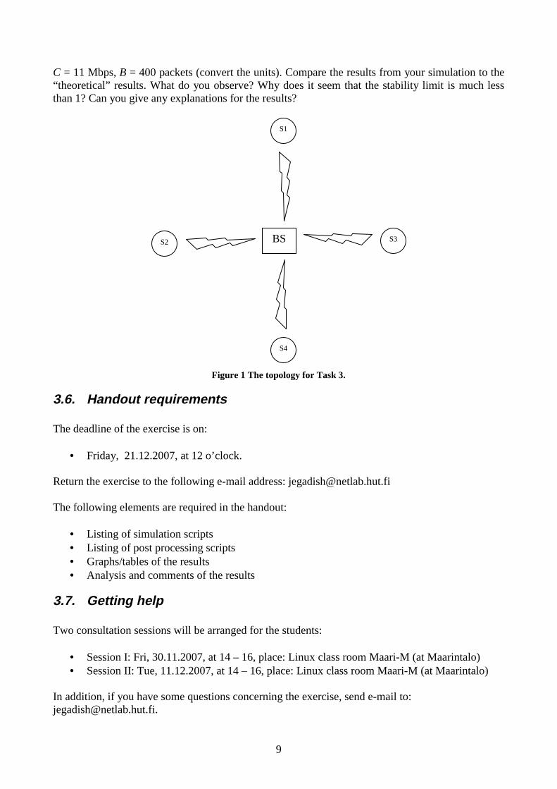
3.5. Task 3 : Load sustained by WLAN under TCP

Refer file: task-3.tcl

In this scenario, there are 5 nodes in the WLAN. One node acts as receiver and the rest of them actas senders. All the senders are at equal distance from the receiver node. In this case we aresimulating the system at the flow level so that flows/file transfers arrive randomly (according to aPoisson process) and the task of TCP is to transfer a file of random size (exponentially distributed).

The script has a parameter to configure the load that need to be generated. Basically, the script usesthe flow inter-arrival time to change the load.

To do:1. Attach 100 TCP sources to each sender node. (So, a total of 400 TCP Agents are created).2. Attach all the TCP sinks to the receiver node (5th Node, node_4). A total of 400 TCP sinks

would be created.3. Set the flow ID (fid_ of TCP Agent) to the agents from 0 to 399. Flow ID values between 0

to 99 correspond to TCP Sender 1 and the next every 100 values correspond to the TCPSender 2, 3 and 4.

4. Attach an FTP Application to each created TCP Agent.5. Set the Packet Size parameter of the TCP Agent to 1460 and the packet count parameter of

FTP Agent to 400.6. Start of the flow generation for each sender node, by calling the 'start flow' procedure. This

is done to set the simulation going.

Measurements to be taken:1. Vary the load (variable rho) from 0.1 to 0.5 (in steps of 0.1).2. The times taken for the file transfers are stored in the array variable 'delres'. Code need to be

added to calculate the average transfer delay (per sender node) by using this values stored inthe variable.

3. The results give you the delay for the flows per node. However, each node is identical, soyou can average also over the results for the different nodes.

4. Remember to implement initial transient control. Also, now you need either batch means orrepeated simulations to construct your 95% confidence intervals.

Also calculate the “theoretical” mean delay assuming that the system would behave as the “ideal”processor sharing model as described in Section 2.3, where the service parameters of the model are

9

C = 11 Mbps,B = 400 packets (convert the units). Compare the results from your simulation to the“theoretical” results. What do you observe? Why does it seem that the stability limit is much lessthan 1? Can you give any explanations for the results?

Figure 1 The topology for Task 3.

3.6. Handout requirements

The deadline of the exercise is on:

• Friday, 21.12.2007, at 12 o’clock.

Return the exercise to the following e-mail address: jegadish@netlab.hut.fi

The following elements are required in the handout:

• Listing of simulation scripts• Listing of post processing scripts• Graphs/tables of the results• Analysis and comments of the results

3.7. Getting help

Two consultation sessions will be arranged for the students:

• Session I: Fri, 30.11.2007, at 14 – 16, place: Linux class room Maari-M (at Maarintalo)• Session II: Tue, 11.12.2007, at 14 – 16, place: Linux class room Maari-M (at Maarintalo)

In addition, if you have some questions concerning the exercise, send e-mail to:jegadish@netlab.hut.fi.

S1

S3

S4

BSS2

10

Appendix

A.1. Installing and using ns2

Ns2 can be built and run both under Unix and Windows. Instructions on how to install ns2 onWindows can be found at:http://www.isi.edu/nsnam/ns/ns-win32-build.html. However, theinstallation may be smoother under Unix.

Modifying ns2

In ns2 it is also possible to modify the existing C++ code or create completely new C++ code. Afterthe changes have been made, the code has to be recompiled by running make in the ns-2.xxdirectory. However, in this exercise you do not have to (and you are not allowed to!) make anychanges at the C++ level, only at the tcl-level.

A.2. General description

Ns2 is an event driven, object oriented network simulator enabling the simulation of a variety oflocal and wide area networks. It implements different network protocols (TCP, UDP), trafficsources (FTP, web, CBR, Exponential on/off), queue management mechanisms (RED, DropTail),routing protocols (Dijkstra) etc. Ns2 is written in C++ and Otcl to separate the control and data pathimplementations. The simulator supports a class hierarchy in C++ (the compiled hierarchy) and acorresponding hierarchy within the Otcl interpreter (interpreted hierarchy).

The reason why ns2 uses two languages is that different tasks have different requirements: Forexample simulation of protocols requires efficient manipulation of bytes and packet headers makingthe run-time speed very important. On the other hand, in network studies where the aim is to varysome parameters and to quickly examine a number of scenarios the time to change the model andrun it again is more important.

In ns2, C++ is used for detailed protocol implementation and in general for such cases where everypacket of a flow has to be processed. For instance, if you want to implement a new queuingdiscipline, then C++ is the language of choice. Otcl, on the other hand, is suitable for configurationand setup. Otcl runs quite slowly, but it can be changed very quickly making the construction ofsimulations easier. In ns2, the compiled C++ objects can be made available to the Otcl interpreter.In this way, the ready-made C++ objects can be controlled from the OTcl level.

There are quite many understandable tutorials available for new ns-users. By going through, forexample, the following tutorials should give you a rather good view of how to create simplesimulation scenarios with ns2:

http://nile.wpi.edu/NS/http://www.isi.edu/nsnam/ns/tutorial/index.html

The next chapters will summarise and explain the key features of tcl and ns2, but in case you needmore detailed information, the ns-manual provides the required information.

http://www.isi.edu/nsnam/ns/ns-documentation.html

11

Other useful ns2 related links, such as archives of ns2 mailing lists, can be found from ns2homepage:

http://www.isi.edu/nsnam/ns/index.html

A.3. Otcl basics

This chapter introduces the syntax and the basic commands of the Otcl language used by ns2. It isimportant that you understand how Otcl works before moving to the chapters handling the creationof the actual simulation scenario.

A.3.1. Assigning values to variables

In tcl, values can be stored to variables and these values can be further used in commands:

set a 5set b [expr $a/5]

In the first line, the variable ‘a’ is assigned the value “5”. In the second line, the result of thecommand [expr $a/5], which equals 1, is then used as an argument to another command, which inturn assigns a value to the variable b. The “$” sign is used to obtain a value contained in a variableand square brackets are an indication of a command substitution.

A.3.2. Procedures

You can define new procedures with the proc command. The first argument to proc is the name ofthe procedure and the second argument contains the list of the argument names to that procedure.For instance a procedure that calculates the sum of two numbers can be defined as follows:

proc sum {a b} {expr $a + $b

}

The next procedure calculates the factorial of a number:

proc factorial a {if {$a <= 1} {

return 1}#here the procedure is called againexpr $x * [factorial [expr $x-1]]}

It is also possible to give an empty string as an argument list. However, in this case the variablesthat are used by the procedure have to be defined as global. For instance:

proc sum {} {global a bexpr $a + $b

}

12

A.3.3. Files and lists

In tcl, a file can be opened for reading with the command:

set testfile [open test.dat r]

The first line of the file can be stored to a list with a command:

gets $testfile list

Now it is possible to obtain the elements of the list with commands (numbering of elements startsfrom 0) :

set first [lindex $list 0]set second [lindex $list 1]

Similarly, a file can be written with a puts command:

set testfile [open test.dat w]puts $testfile “testi”

A.3.4. Calling subprocesses

The command exec creates a subprocess and waits for it to complete. The use of exec is similar togiving a command line to a shell program. For instance, to remove a file:

exec rm $testfile

The exec command is particularly useful when one wants to call a tcl-script from within another tcl-script. For instance, in order to run the tcl-script example.tcl multiple times with the value of theparameter “test” ranging from 1 to 10, one can type the following lines to another tcl-script:

for {set ind 1} {$ind <= 10} {incr ind} {

set test $indexec ns example.tcl test

}

A.4. Creating the topology

To be able to run a simulation scenario, a network topology must first be created. In ns2, thetopology consists of a collection of nodes and links.

Before the topology can be set up, a new simulator object must be created at the beginning of thescript with the command:

set ns [new Simulator]

13

The simulator object has member functions that enable creating the nodes and the links, connectingagents etc. All these basic functions can be found from the class Simulator. When using functionsbelonging to this class, the command begins with “$ns”, since ns was defined to be a handle to theSimulator object.

A.4.1. Nodes

New node objects can be created with the command

set n0 [$ns node]set n1 [$ns node]set n2 [$ns node]set n3 [$ns node]

The member function of the Simulator class, called “node” creates four nodes and assigns them tothe handles n0, n1, n2 and n3. These handles can later be used when referring to the nodes. If thenode is not a router but an end system, traffic agents (TCP, UDP etc.) and traffic sources (FTP,CBR etc.) must be set up, i.e, sources need to be attached to the agents and the agents to the nodes,respectively.

A.4.2. Agents, applications and traffic sources

The most common agents used in ns2 are UDP and TCP agents. In case of a TCP agent, severaltypes are available. The most common agent types are:

• Agent/TCP – a Tahoe TCP sender• Agent/TCP/Reno – a Reno TCP sender• Agent/TCP/Sack1 – TCP with selective acknowledgement

The most common applications and traffic sources provided by ns2 are:

• Application/FTP – produces bulk data that TCP will send• Application/Traffic/CBR – generates packets with a constant bit rate• Application/Traffic/Exponential – during off-periods, no traffic is sent. During on-periods,

packets are generated with a constant rate. The length of both on and off-periods isexponentially distributed.

• Application/Traffic/Trace – Traffic is generated from a trace file, where the sizes andinterarrival times of the packets are defined.

In addition to these ready-made applications, it is possible to generate traffic by using the methodsprovided by the class Agent. For example, if one wants to send data over UDP, the method

send(int nbytes)

can be used at the tcl-level provided that the udp-agent is first configured and attached to somenode.

14

Below is a complete example of how to create a CBR traffic source using UDP as transport protocoland attach it to node n0:

set udp0 [new Agent/UDP]$ns attach-agent $n0 $udp0set cbr0 [new Application/Traffic/CBR]$cbr0 attach-agent $udp0$cbr0 set packet_size_ 1000$cbr0 set rate_ 1000000

An FTP application using TCP as a transport protocol can be created and attached to node n1 inmuch the same way:

set tcp1 [new Agent/TCP]$ns attach-agent $n1 $tcp1set ftp1 [new Application/FTP]$ftp1 attach-agent $tcp1$tcp1 set packet_size_ 1000

The UDP and TCP classes are both child-classes of the class Agent. With the expressions [newAgent/TCP] and [new Agent/UDP] the properties of these classes can be combined to the newobjects udp0 and tcp1. These objects are then attached to nodes n0 and n1. Next, the application isdefined and attached to the transport protocol. Finally, the configuration parameters of the trafficsource are set. In case of CBR, the traffic can be defined by parameters rate_ (or equivalentlyinterval_, determining the interarrival time of the packets), packetSize_ and random_ . With therandom_ parameter it is possible to add some randomness in the interarrival times of the packets.The default value is 0, meaning that no randomness is added.

A.4.3. Traffic Sinks

If the information flows are to be terminated without processing, the udp and tcp sources have to beconnected with traffic sinks. A TCP sink is defined in the class Agent/TCPSink and an UDP sink isdefined in the class Agent/Null.

A UDP sink can be attached to n2 and connected with udp0 in the following way:

set null [new Agent/Null]$ns attach-agent $n2 $null$ns connect $udp0 $null

A standard TCP sink that creates one acknowledgement per a received packet can be attached to n3and connected with tcp1 with the commands:

set sink [new Agent/Sink]$ns attach-agent $n3 $sink$ns connect $tcp1 $sink

There is also a shorter way to define connections between a source and the destination with thecommand:

15

$ns create-connection <srctype> <src> <dsttype> <dst> <pktclass>

For example, to create a standard TCP connection between n1 and n3 with a class ID of 1:

$ns create-connection TCP $n1 TCPSink $n3 1

One can very easily create several tcp-connections by using this command inside a for-loop.

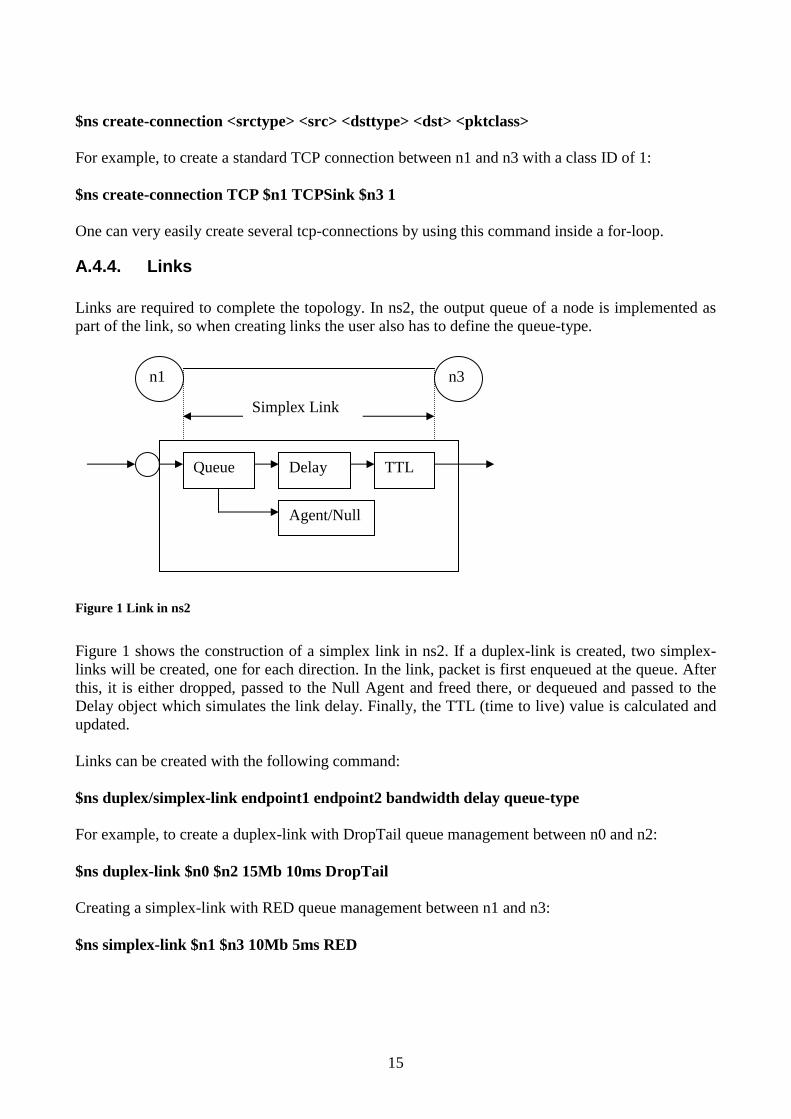
A.4.4. Links

Links are required to complete the topology. In ns2, the output queue of a node is implemented aspart of the link, so when creating links the user also has to define the queue-type.

Figure 1 Link in ns2

Figure 1 shows the construction of a simplex link in ns2. If a duplex-link is created, two simplex-links will be created, one for each direction. In the link, packet is first enqueued at the queue. Afterthis, it is either dropped, passed to the Null Agent and freed there, or dequeued and passed to theDelay object which simulates the link delay. Finally, the TTL (time to live) value is calculated andupdated.

Links can be created with the following command:

$ns duplex/simplex-link endpoint1 endpoint2 bandwidth delay queue-type

For example, to create a duplex-link with DropTail queue management between n0 and n2:

$ns duplex-link $n0 $n2 15Mb 10ms DropTail

Creating a simplex-link with RED queue management between n1 and n3:

$ns simplex-link $n1 $n3 10Mb 5ms RED

n1 n3

Queue Delay TTL

Agent/Null

Simplex Link

16

The values for bandwidth can be given as a pure number or by using qualifiers k (kilo), M (mega), b(bit) and B (byte). The delay can also be expressed in the same manner, by using m (milli) and u(mikro) as qualifiers.

There are several queue management algorithms implemented in ns2, but in this exercise onlyDropTail and RED will be needed.

A.5. Adding loss modules

You can create packet losses artificially by adding a separate loss module to a link. The loss modulecan be created and configured as follows:

# create a random variable that follows the uniform distributionset loss_random_variable [new RandomVariable/Uniform]$loss_random_variable set min_ 0 # the range of the random variable;$loss_random_variable set max_ 100

set loss_module [new ErrorModel] # create the error model;$loss_module drop-target [new Agent/Null] #a null agent where the dropped packets go to$loss_module set rate_ 10 # error rate will then be (0.1 = 10 / (100 - 0));$loss_module ranvar $loss_random_variable # attach the random variable to loss module;

You can attach the loss module to a certain link between two nodes, n1 and n2, with the command:

$ns lossmodel $loss_module $n1 $n2

A.6. Tracing and monitoring

In order to be able to calculate the results from the simulations, the data has to be collectedsomehow. Ns2 supports two primary monitoring capabilities: traces and monitors. The traces enablerecording of packets whenever an event such as packet drop or arrival occurs in a queue or a link.The monitors provide a means for collecting quantities, such as number of packet drops or numberof arrived packets in the queue. The monitor can be used to collect these quantities for all packets orjust for a specified flow (a flow monitor)

A.6.1. Traces

All events from the simulation can be recorded to a file with the following commands:

set trace_all [open all.dat w]$ns trace-all $trace_all$ns flush-traceclose $trace_all

First, the output file is opened and a handle is attached to it. Then the events are recorded to the filespecified by the handle. Finally, at the end of the simulation the trace buffer has to be flushed andthe file has to be closed. This is usually done with a separate finish procedure.

17

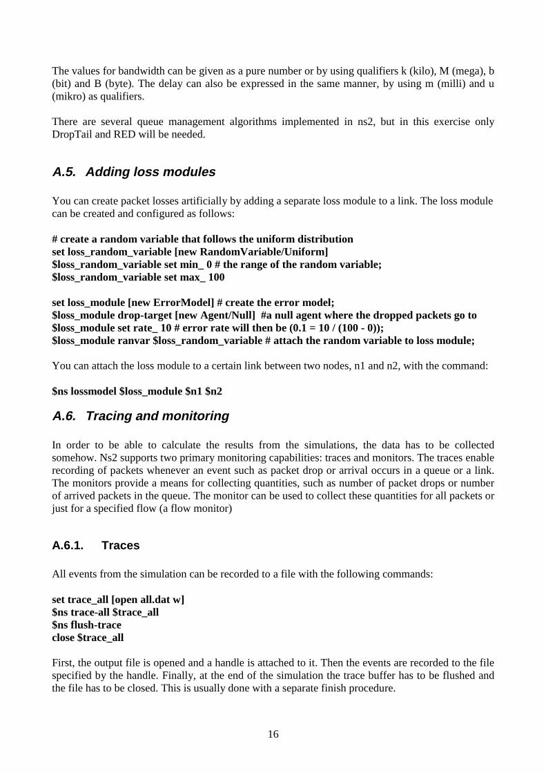
If links are created after these commands, additional objects for tracing (EnqT, DeqT, DrpT andRecvT) will be inserted into them.

Figure 2 Link in ns2 when tracing is enabled

These new objects will then write to a trace file whenever they receive a packet. The format of thetrace file is following:

+ 1.8437 5 0 2 cbr 210 ------- 0 0.0 3.1 225 610- 1.8437 5 0 2 cbr 210 ------- 0 0.0 3.1 225 610r 1.8447 1 2 1 cbr 210 ------- 1 3.0 1.0 195 600r 1.8456 6 2 0 ack 40 ------- 2 3.2 0.1 82 602+ 1.8456 6 0 2 tcp 1000 ------- 2 0.1 3.2 102 611- 1.8456 6 0 2 tcp 1000 ------- 2 0.1 3.2 102 611

+ : enqueue- : dequeued : dropr : receive

The fields in the trace file are: type of the event, simulation time when the event occurred, sourceand destination nodes, packet type (protocol, action or traffic source), packet size, flags, flow id,source and destination addresses, sequence number and packet id.

In addition to tracing all events of the simulation, it is also possible to create a trace object betweena particular source and a destination with the command:

$ns create-trace type file src dest

where the type can be, for instance,

• Enque – a packet arrival (for instance at a queue)• Deque – a packet departure (for instance at a queue)• Drop – packet drop• Recv – packet receive at the destination

Tracing all events from a simulation to a specific file and then calculating the desired quantitiesfrom this file for instance by using perl or awk and Matlab is an easy way and suitable when thetopology is relatively simple and the number of sources is limited. However, with complextopologies and many sources this way of collecting data can become too slow. The trace files willalso consume a significant amount of disk space.

Queue Delay TTL

Agent/Null

EnqT DeqT

DrpT

RecvT

18

A.6.2. Monitors

With a queue monitor it is possible to track the statistics of arrivals, departures and drops in eitherbytes or packets. Optionally the queue monitor can also keep an integral of the queue size overtime.

For instance, if there is a link between nodes n0 and n1, the queue monitor can be set up as follows:

set qmon0 [$ns monitor-queue $n0 $n1 stdout]

The monitor does not automatically produce any trace data. The above command just prepares thequeue for maintaining certain statistics. For example, the packet arrivals and byte drops can be readwith the commands (executing these would have to be scheduled for a certain time):

set parr [$qmon0 set parrivals_]set bdrop [$qmon0 set bdrops_]

Notice that besides assigning a value to a variable the set command can also be used to get the valueof a variable. For example here the set command is used to get the value of the variable “parrivals”defined in the queue monitor class.

A flow monitor is similar to the queue monitor but it keeps track of the statistics for a flow ratherthan for aggregated traffic. A classifier first determines which flow the packet belongs to and thenpasses the packet to the flow monitor.

The flowmonitor can be created and attached to a particular link with the commands:

set fmon [$ns makeflowmon Fid]$ns attach-fmon [$ns link $n1 $n3] $fmon

Notice that since these commands are related to the creation of the flow-monitor, the commands aredefined in the Simulator class, not in the Flowmonitor class. The variables and commands in theFlowmonitor class can be used after the monitor is created and attached to a link. For instance, todump the contents of the flowmonitor (all flows):

$fmon dump

If you want to track the statistics for a particular flow, a classifier must be defined so that it selectsthe flow based on its flow id, which could be for instance 1:

set fclassifier [$fmon classifier]set flow [$fclassifier lookup auto 0 0 1]

In this exercise all relevant data concerning packet arrivals, departures and drops should be obtainedby using monitors. If you want to use traces, then at least do not trace all events of the simulation,since it would be highly unnecessary. However, it is still recommended to use the monitors, sincewith the monitors you will directly get the total amount of events during a specified time interval,whereas with traces you will have to parse the output file to get these quantities.

19

A.7. Controlling the simulation

After the simulation topology is created, agents are configured etc., the start and stop of thesimulation and other events have to be scheduled.

The simulation can be started and stopped with the commands

$ns at $simtime “finish”$ns run

The first command schedules the procedure finish at the end of the simulation, and the secondcommand actually starts the simulation. The finish procedure has to be defined to flush the tracebuffer, close the trace files and terminate the program with the exit routine. It can optionally startNAM (a graphical network animator), post process information and plot this information.

The finish procedure has to contain at least the following elements

proc finish {} {global ns trace_all$ns flush-traceclose $trace_allexit 0

}

Other events, such as the starting or stopping times of the clients can be scheduled in the followingway:

$ns at 0.0 “cbr0 start”$ns at 50.0 “ftp1start”$ns at $simtime “cbr0 stop”$ns at $simtime “ftp1 stop”

If you have defined your own procedures, you can also schedule the procedure to start for exampleevery 5 seconds in the following way:

proc example {} {global nsset interval 5….…$ns at [expr $now + $interval] “example”

}

A.8. Simple ns2 example

To give you a better idea of how these pieces can be put together, a very simple example script isgiven here. The script in itself does not do anything meaningful, the purpose is just to show youhow to construct a simulation.

20

n0 n2n1

3 Mbps1 ms

5 Mbps15 ms

The script first creates the topology shown in Figure 3 and then adds one CBR traffic source usingUDP as transport protocol and records all the events of the simulation to a trace file.

Figure 3 Example simulation topology

The example script:

#Creation of the simulator objectset ns [new Simulator]

#Enabling tracing of all events of the simulationset f [open out.all w]$ns trace-all $f

#Defining a finish procedure

proc finish {} {global ns f$ns flush-traceclose $fexit0

}

#Creation of the nodesset n0 [$ns node]set n1 [$ns node]set n2 [$ns node]

#Creation of the links$ns duplex-link $n0 $n1 3Mb 1ms DropTail$ns duplex-link $n0 $n1 1Mb 15ms DropTail

#Creation of a cbr-connection using UDPset udp0 [new Agent/UDP]$ns attach-agent $n0 $udp0set cbr0 [new Application/Traffic/CBR]$cbr0 attach-agent $udp0$cbr0 set packet_size_ 1000$udp0 set packet_size_ 1000$cbr0 set rate_ 1000000$udp0 set class_ 0

set null0 [new Agent/Null]

21

$ns attach-agent $n2 $null0$ns connect $udp0 $null0

#Scheduling the events$ns at 0.0 “$cbr0 start”$ns at $simtime “$cbr0 stop”

$ns at $simtime “finish”

$ns run