econstorMake Your Publications Visible.

A Service of

zbwLeibniz-InformationszentrumWirtschaftLeibniz Information Centrefor Economics

Headey, Bruce; Muffels, Ruud

Working Paper

Two-way Causation in Life Satisfaction Research:Structural Equation Models with Granger-Causation

IZA Discussion Papers, No. 8665

Provided in Cooperation with:IZA – Institute of Labor Economics

Suggested Citation: Headey, Bruce; Muffels, Ruud (2014) : Two-way Causation in LifeSatisfaction Research: Structural Equation Models with Granger-Causation, IZA DiscussionPapers, No. 8665, Institute for the Study of Labor (IZA), Bonn

This Version is available at:http://hdl.handle.net/10419/106605

Standard-Nutzungsbedingungen:

Die Dokumente auf EconStor dürfen zu eigenen wissenschaftlichenZwecken und zum Privatgebrauch gespeichert und kopiert werden.

Sie dürfen die Dokumente nicht für öffentliche oder kommerzielleZwecke vervielfältigen, öffentlich ausstellen, öffentlich zugänglichmachen, vertreiben oder anderweitig nutzen.

Sofern die Verfasser die Dokumente unter Open-Content-Lizenzen(insbesondere CC-Lizenzen) zur Verfügung gestellt haben sollten,gelten abweichend von diesen Nutzungsbedingungen die in der dortgenannten Lizenz gewährten Nutzungsrechte.

Terms of use:

Documents in EconStor may be saved and copied for yourpersonal and scholarly purposes.

You are not to copy documents for public or commercialpurposes, to exhibit the documents publicly, to make thempublicly available on the internet, or to distribute or otherwiseuse the documents in public.

If the documents have been made available under an OpenContent Licence (especially Creative Commons Licences), youmay exercise further usage rights as specified in the indicatedlicence.

www.econstor.eu

DI

SC

US

SI

ON

P

AP

ER

S

ER

IE

S

Forschungsinstitut zur Zukunft der ArbeitInstitute for the Study of Labor

Two-way Causation in Life Satisfaction Research: Structural Equation Models with Granger-Causation

IZA DP No. 8665

November 2014

Bruce HeadeyRuud Muffels

Two-way Causation in Life Satisfaction Research: Structural Equation Models

with Granger-Causation

Bruce Headey Melbourne University

Ruud Muffels

Tilburg University and IZA

Discussion Paper No. 8665 November 2014

IZA

P.O. Box 7240 53072 Bonn

Germany

Phone: +49-228-3894-0 Fax: +49-228-3894-180

E-mail: iza@iza.org

Any opinions expressed here are those of the author(s) and not those of IZA. Research published in this series may include views on policy, but the institute itself takes no institutional policy positions. The IZA research network is committed to the IZA Guiding Principles of Research Integrity. The Institute for the Study of Labor (IZA) in Bonn is a local and virtual international research center and a place of communication between science, politics and business. IZA is an independent nonprofit organization supported by Deutsche Post Foundation. The center is associated with the University of Bonn and offers a stimulating research environment through its international network, workshops and conferences, data service, project support, research visits and doctoral program. IZA engages in (i) original and internationally competitive research in all fields of labor economics, (ii) development of policy concepts, and (iii) dissemination of research results and concepts to the interested public. IZA Discussion Papers often represent preliminary work and are circulated to encourage discussion. Citation of such a paper should account for its provisional character. A revised version may be available directly from the author.

IZA Discussion Paper No. 8665 November 2014

ABSTRACT

Two-way Causation in Life Satisfaction Research:

Structural Equation Models with Granger-Causation* Two-way causation issues are the bete noire of life satisfaction research. As acknowledged in several landmark reviews, many variables routinely reported as causes or determinants of life satisfaction could equally well be consequences, or perhaps both causes and consequences (Diener, 1984; Diener, Suh, Lucas and Smith, 1999; Argyle, 2001; Frey and Stutzer, 2002). These variables include one’s state of health, social support and participation, exercise, job satisfaction and satisfaction with one’s partner and family life. In previous attempts to disentangle two-way causation issues, a wide variety of statistical models have been deployed. Conflicting empirical results have been reported, together with concerns about model ‘goodness of fit’ and model stability. In this paper we estimate five-wave structural equation models using data from large, nationally representative panel surveys in Australia, Britain and Germany. The models are based on a modified concept of Granger-causation (Granger, 1969). The main intuition behind Granger-causation is that if lagged versions of time-series variable x have statistically significant effects on time-series variable y in equations in which multiple lagged versions of y are also included, then it can be inferred that x is one cause (or ‘Granger-cause’) of y. We adapt Granger’s approach, extending it to encompass two-way causation and panel survey data. It transpires that our Granger-style models have satisfactory fits to the panel data and are stable. Alternative models fit the data much less well. Substantively, we find that two-way causation is pervasive: all of the x variables mentioned above appear to be both causes and consequences of life satisfaction. With minor exceptions, results replicate across all three datasets, despite non-trivial differences between the measures used in the three countries. One implication is that researchers who have assumed one-way causation have seriously over-estimated the effects of x variables on LS. A second implication is that many people apparently experience multi-year gains or losses of life satisfaction rather than just recording short term fluctuations around their own normal level or ‘set-point’. JEL Classification: J01, I12, I31 Keywords: life satisfaction, health, job satisfaction and social behaviours,

two-way causation, Granger-causation, panel surveys Corresponding author: Bruce Headey Melbourne Institute of Applied Economic and Social Research Level 5, Faculty of Business and Economics Building 111 Barry Street University of Melbourne Australia E-mail: b.headey@unimelb.edu.au

* We would like to thank Ulrich Schimmack of the University of Toronto at Mississauga and Derek Headey of the International Food Policy Research Institute (IFPRI) for helpful suggestions on modelling reciprocal causation.

3

1. INTRODUCTION

The purpose of this paper is to propose a modified Granger-causation model

(Granger, 1969) to assess possible two-way causation between life satisfaction (LS)

and a range of x variables. The selected x’s are intended to be reasonably

representative of variables usually reported as determinants or causes of LS: health,

social networks and social participation, exercise, job satisfaction and satisfaction

with family life. Models are estimated using data from three long-running national

panel surveys: the Household Income and Labour Dynamics Australia (HILDA)

Survey, the British Household Panel Survey (BHPS) and the German Socio-

Economic Panel Survey (SOEP).

The agreed focus of most LS research is on explaining why some people are more

satisfied with life (happier) than others. So, with a few notable exceptions (e.g. Deeg

& van Zonneveld, 1989; Veenhoven, 1989), the research literature is about presumed

causes of LS. But, as has been recognised in major reviews of the field, many of the

variables usually reported as causes could be consequences, or perhaps both causes

and consequences (Diener, 1984; Diener, Suh, Lucas & Smith, 1999; Argyle, 2001;

Frey & Stutzer, 2002). The tendency to sweep two-way causation issues under the

carpet in empirical work can lead to logical contradictions. For example, one’s state

of health is routinely reported to be a major determinant of happiness, particularly in

older age groups (Gerstorf et al., 2008), but it is also well established that happy

people live longer than unhappy people, even controlling for state of health at baseline

(Deeg & van Donneveld, 1989; Headey, Hoehne & Wagner, 2013). It follows that

happiness must have the effect of promoting better health; otherwise happy people

would not live longer. In this paper, the first models we estimate relate to health and

happiness, and we find that there is, indeed, clear evidence of two-way causation.

Difficult epistemological and statistical issues arise, as soon as one tries to

conceptualize and then estimate two-way causation models. First, some terminology:

in reviewing the field, Diener and colleagues (Diener, 1984, Diener, Suh, Lucas &

Smith, 1999) distinguish between bottom-up (BU) and top-down (TD) models of LS.

In bottom-up models overall LS or happiness is viewed as the outcome variable and

other variables (e.g. health, social support) are conceived of as causes of LS. In top-

4

down models these latter variables are conceived of as consequences (one might say

‘spin-offs’) of overall LS. Extending this framework, other researchers have

suggested that some variables may be both causes and consequences of LS (e.g.

Lance, Lautenschlager, Sloan & Varca, 1989; Headey, Veenhoven & Wearing, 1991).

That is, it is possible that changes over time in x could lead to changes in LS, and that

changes in LS could lead to changes in x. For example, changes in job satisfaction or

health satisfaction could lead to changes in LS, and changes in LS could have spin-off

effects on job or health satisfaction, and possibly on satisfaction with other domains

of life too. A final possibility is that apparent links between changes in x and changes

in LS could be spurious, due to omitted variables bias.

Figure 1 illustrates these possibilities in the context of a model based on just three

waves of panel data, rather than the five waves used in this paper. In the causal

modelling literature, this type of model is known as a cross-lagged panel model,

because of the criss-cross links between x and LS.

Insert Figure 1 here

Assuming that there is a statistically significant correlation (or covariance) between

an x variable and LS, four sets of results are possible when the Figure 1 model is

estimated. One possibility is that BU links from x to LS are found to be statistically

significant, but not TD links. The reverse possibility may also be found. A third

possibility is two-way causation in that both BU and TD links are significant. The

final possibility is a model in which links between x and LS are wholly or partly

spurious. In a wholly spurious model, only the curved two-way links marked SP in

Figure 1 would be significant. As explained in the Methods section, these links

represent correlations between the error terms of a structural equation for LS and an

equation for an x variable. If SP is statistically significant, it is likely due to the effects

of variables omitted from the model (presumably because not measured), which affect

both LS and x.

A crucial point here is that all four possible outcomes must be allowed for in

empirical modelling. An approach that, by accident or design, precludes the empirical

possibility of finding one or more of these outcomes is seriously flawed. As will

5

become clear in the literature review below, some previous approaches are flawed for

this reason.

We next consider some merits and limitations of Granger-causation (Granger, 1969,

Granger & Newbold, 1974; Pearl, 2009). The key intuition behind the concept of

Granger-causation for which Clive Granger won the Noble Prize in Economics in

2003, is that multiple lags, rather than just a single lag of both an x variable and an

outcome variable should initially be included in one’s models. Then if any lag of the x

variable is found to be statistically, significantly related to the outcome variable, x

may reasonably be regarded as one cause (although presumably not the only cause) of

the outcome variable. Granger suggested both substantive and methodological

reasons for including multiple lags. Substantively, multiple lags are worth including

because results at time t may depend on results at t-2, t-3 etc as well as t-1. For

example, people may be more likely to experience a high level of LS at time t, if they

were relatively happy at t-2 or t-3 etc, even net of the effect of their happiness at t-1.

The same could be hypothesized in relation to health, poverty and many other

phenomena studied by social scientists. Methodologically, one benefit of including

multiple lags may be to reduce the effects of omitted variables bias which influence

both x and y, and whose effects might lead the researcher to conclude that x caused y,

when in fact the relationship was spurious (Granger & Newbold, 1974; Finkel, 1995).

Granger-causation has originally been proposed for analysis of long time-series data

in which numerous observations of an x variable and a y variable were available, and

the question was: “Is x a cause of y?”. Our suggestion in this paper is to extend

Granger’s approach to issues of two-way causation and to panel survey data. In

practice, we shall find that our adapted Granger models are an excellent fit to the

three-nation panel data. Inclusion of additional lags of dependent variables improves

model fit, over and above what is achieved by including only single lags. The four

dotted arrows in Figure 1 represent the only “Granger” lags that can be added to a

three-wave panel model. However, the reader is asked to envisage the extra lags

between all previous waves of x and y and all later waves, which can be included in

our five-wave models.

Another important issue to consider in causal modelling is the time lag between

changes in an explanatory variable and changes in the outcome variable. A ‘common

6

sense’ view, which underlies Granger-causation and most other accounts of causation,

is that causes must precede effects. In Figure 1 it is implicitly assumed that changes in

x affect changes in LS after some discrete time lag, and that changes in LS, if they

affect x at all, also take effect after a time lag. However, in considering our data, it is

plausible to believe that the effects of x variables on LS might well be (a) continuous

and/or (b) simultaneous or almost simultaneous. As an example, consider possible

two-way effects between job satisfaction and LS. It is reasonable to suppose that these

two-way effects (if significant at all) are continuous and almost simultaneous. In the

case of changes in social support, on the other hand, effects might be more or less

continuous, but probably not simultaneous.1

It can be shown mathematically that, if effects are continuous, cross-lagged models of

the kind shown in Figure 1 – and, by extension, Granger models - yield unbiased and

consistent estimates of the relevant coefficients (Coleman, 1968; Tuma and Hannan,

1984; Finkel, 1995). The point is that, if effects are continuous, the time points at

which panel survey measurements are taken are arbitrary, and the task of the

researcher is to recover the coefficients of change, using calculus:

0 1 2

3 4 5

(1.1)

(1.2)

iti it i it

iti it i it

dy x ydt

dx y xdt

γ γ γ

γ γ γ

= + +

= + +

These two differential equations state that instantaneous rates of change for each

individual i (the coefficients) in xi and yi are dependent on each other over time

(Coleman, 1968; Tuma and Hannan, 1984; Finkel, 1995). Straighforward

mathematics show that these equations are equivalent to the standard structural

equations (2.1 and 2.2 below) for two-way cross-lagged causation between x and y,

except that in the structural equations random error terms are added to take account of

omitted variables.

1 i.e. one might expect a time delay before a loss of social support affected LS, or a decline in LS affected social support.

7

1 1 1 2 1 1

2 3 1 4 1 2

(2.1) (2.2)

it it it i

it it it i

y x y ex y x e

α β βα β β

− −

− −

= + + += + + +

The structural equations can be estimated to provide unbiased and consistent

estimates of the continuous effect of x on y and y on x (Finkel, 1995).

Finally, we need to discuss additional modelling issues which arise because the

changes we are considering may be not just continuous, but also simultaneous. In

Granger-causation it is assumed that causes precede effects, so strictly speaking,

Granger’s approach cannot be extended to simultaneous causation (Pearl, 2009).

However, the word ‘simultaneous’ should not be taken absolutely literally in this

context. The causal influences in question could be almost simultaneous, or more

practically, could take effect at an interval considerably shorter than the length of time

between panel surveys (Finkel, 1995). It might be thought that the way to deal with

this possibility would be just to add simultaneous causal links to the model in Figure

1. Unfortunately, models with both simultaneous and cross-lagged links cannot

usually, in practice, be estimated. This is due to problems both of under-identification

and multicollinearity (Kessler and Greenberg, 1981; Finkel, 1995).2 A practical, fall-

back procedure that can be followed if, as we found here, a model of this type cannot

be estimated is to estimate a model with only simultaneous links, and then compare

results with those from a model with only cross-lagged links, or by extension,

Granger-links (Greenberg and Kessler, 1982). If the signs of coefficients of interest in

both models are the same, and the coefficients are also statistically significant, then

the researcher can feel reassured that results are consistent with each other, although if

the ‘true’ causal (time) lag is misspecified in both models, coefficients are likely to be

under-estimates. This procedure was followed in the present paper and, as reported in

detail below, the BU and TD estimates of main interest were always consistent. More

2 Kessler and Greenberg (1981, chap. 3) describe how a multi-wave panel model of this kind may in principle be identified by using equality constraints (i.e. by constraining sets of parameters to be equal to each other). In practice, this approach to identification only succeeds if relationships among variables are quite far from equilibrium (i.e. relationships differ substantially from wave to wave of the panel data). In panel surveys of life satisfaction, it is reasonably clear that relationships between LS and causal variables of interest are much the same from wave to wave. Estimation of models with both simultaneous and cross-lagged links is also likely to run into problems because of multicollinearity; the effects on LS of x at time t and x at t-1 are likely to be too highly correlated for estimates to be reliable.

8

to the point, the Granger-style models were in all cases a much better fit to the data

than models with only cross-lagged links or only simultaneous links.

2. PREVIOUS RESEARCH ON TWO-WAY CAUSATION

The first investigations of two-way causation focussed on links between LS and

domain satisfactions, including job satisfaction, marital satisfaction and satisfaction

with social activities. Cross-sectional data were analysed (not panel data), so

equations had to be statistically identified by using instrumental variables (Schmitt

and Bedeian, 1982; Lance et al, 1989; Lance, Mallard and Michalos, 1995). The main

requirements for valid instruments are that (a) the variable(s) used to identify the y

equation have to be substantially correlated with y, but only linked indirectly to y via x

and, similarly, (b) the variable(s) used to identify the x equation have to be

substantially correlated with x but only linked to x indirectly via y. In practice, it is

usually difficult to find valid instruments. The instruments used in the first

investigations of two-way causation included demographic variables like age and

marital status, measures of social support and personality traits. The results generally

suggested two-way causation between LS and domain satisfactions but it is hard to be

convinced that the instruments were valid.3

From the 1990s onwards most investigations of two-way causation used panel survey

data. If two or more waves of panel data are available, a cross-lagged model (see

Figure 1) is bound to be identified, because lagged versions of the dependent variable

in each equation serve as instruments (Kessler and Greenberg, 1981; Finkel, 1995). If

three or more waves are available, a simultaneous causation model can also be

identified by using equality constraints (Kessler and Greenberg, 1981). Headey,

Veenhoven and Wearing (1991) used four waves of panel data to assess two-way

links between LS and domain satisfactions. They compared results from cross-lagged

and simultaneous causation models, finding that the simultaneous models were a

better fit to the data. They reported two-way causation between marital satisfaction

and LS, and top-down causation from LS to job satisfaction, leisure satisfaction, and

3 The main difficulty in these studies lay in finding instruments for LS. Age, marital status and personality traits were used. It seems likely that these variables would be directly related to domain satisfactions, as well as LS.

9

satisfaction with one’s standard of living. The association between LS and

satisfaction with friendships appeared to be spurious.

Scherpenzeel and Saris (1996) cast doubt on previous results in analyses based on

four Dutch surveys, three of which were panels. They assessed links between LS and

satisfaction with one’s housing, financial situation and social contacts. Analysing the

panel studies, they estimated cross-lagged models, using as instruments both lagged

versions of dependent variables and exogenous demographic variables. Their main

conclusion was that results were not stable from dataset to dataset, and also varied

depending on which specific variables were used as instruments. They viewed their

analysis as showing that even a multi-wave panel approach is fundamentally flawed,

because stable results cannot be obtained.

Against this view, it seems fair to point out that, if one conducts two and three-wave

panel surveys within the course of a single year, little or no real change is likely to

occur in the lives of most respondents, so unstable model estimates are not

unexpected.4 Also, although the authors state whether models with BU, or TD or two-

way links provided the best Chi-square fit for each domain satisfaction in each

dataset, they give no details, so it is not possible for readers to assess which if any of

the model fits was satisfactory. A further observation is that, contrary to standard

structural equation modelling procedure, they did not estimate correlations between

the error terms of equations for LS and domain satisfactions (see Figure 1; the curved

links marked SP). That is, they did not specifically allow for the possibility that some

apparently significant BU or TD links might be spurious, due to omitted variables.

This would usually lead to biased over-estimation of BU and TD links. Experience in

modelling LS data also suggests that omission of these correlated error terms often

results in models with unacceptably poor fits.

A carefully designed study of links between health (the Health SF-36 scale; Ware,

Snow and Kosinski, 2000) and perceived quality of life was undertaken by Mathison

et al (2007). They collected four waves of panel data from about 170 patients before

and after heart surgery. Structural equation models with cross-lagged and

4 The authors report that in two of the panel surveys interviews were conducted only a few weeks apart.

10

simultaneous links were estimated separately. Both models indicated significant two-

way causation between health and perceived quality of life. The fit of the models to

the data was satisfactory, with the simultaneous model having a closer fit.

Two-way linkages have been consistently reported in studies of volunteering and LS.

Thoits and Hewitt (2001) undertook a two-wave panel study and reported significant

cross-lagged links. In Kuskova’s (2011) four-wave panel which investigated

volunteering by company employees, there were stronger TD links from LS to

volunteering than the other way round, but both links were statistically significant.

Meier and Stutzer (2004) sought to address the same issues in a quasi-experimental

study. They observed that when communism collapsed in East Germany in 1989, an

elaborate volunteering structure also collapsed. Using SOEP data, they showed that

those who managed to remain as volunteers in reunified Germany were significantly

more satisfied with life, net of their pre-unification scores, than people who ceased to

be volunteers. However, TD links from LS to volunteering also proved to be

statistically significant. Also using a quasi-experimental design, and SOEP data,

Nagazato, Schimmack and Oishi (2011) assessed the effects of recent house moves on

housing satisfaction and LS. Their cross-lagged model, using two waves of data,

indicated two-way causation. Their two-way model had a satisfactory fit to the data

and was clearly preferable to a BU or TD model.

In summary, previous research has not yielded entirely consistent results, but in

general leads us to hypothesize that two-way causal relationships will be found

between overall LS and variables substantially correlated with it. In assessing these

relationships, it is crucial to estimate models which allow for the empirical possibility

of finding one of four alternatives: (1) only BU links are statistically significant (2)

only TD links are significant (3) both BU and TD links are significant (i.e. there is

two-way causation), or (4) only SP links are significant (i.e. correlations between LS

and the x variable are spurious). It should also be clear that different alternatives -

different patterns of causation - could be found for different x variables.

From a methodological standpoint, our aim is to compare the model fit and stability of

Granger-style models – models with multiple lags – with one-way causation models

and also with the two main two-way causation alternatives deployed in previous

research, namely cross-lagged panel models and simultaneous causation panel

11

models. Again, it is possible that results could differ from x variable to x variable. It

will be a bonus if one type of model is the best fit for all variables.

All of the x variables selected for inclusion in our structural equation models are

usually listed as causes of LS. A person’s state of health, whether self-rated or

measured objectively by physicians or tests, is invariably found to be positively

associated with LS (Schwarze, 2000). However, subjective/self-rated measures are

much more highly correlated than objective ones (Ambrasat, Schupp and Wagner,

2011), which itself suggests some degree of TD causation. Among the strongest

findings in the first empirical studies of LS was that the quality of a person’s social

support, and also frequency of participation in social activities with friends and

acquaintances, are strongly associated with happiness (Bradburn, 1969; Andrews and

Withey, 1976; Campbell, Converse and Rodgers, 1976). Regular exercise is not

routinely listed among possible causes of LS, but has been shown to be associated

with LS even in fixed effects models (Headey, Muffels and Wagner, 2010; 2012).

Finally, job satisfaction and satisfaction with one’s partner/marriage and family life

are always found to strongly related to LS… but researchers sometimes note that

issues of causal direction are unresolved.

3. METHODS

This section is in three parts. We briefly describe the three national household panel

surveys, which are our data sources. Then we describe the main measures used: LS

and the x variables. Then comes a longer section on contentious issues involved in

modelling two-causation.

Three long-running national household panel surveys

The Household Income and Labour Dynamics Australia (HILDA) Survey

The HILDA panel began in 2001 with a sample of 13,969 individuals in 7,700

households (Watson and Wooden, 2004). Interviews were achieved in 61% of in-

scope households. In the Australian panel all household members aged 15 and over

are interviewed. The cross-sectional representativeness of the panel is maintained by

interviewing ‘split-offs’ and their new families. So when a young person leaves home

(‘splits off’) to marry and set up a new family, the entire new family becomes part of

12

the panel. It may be noted that, as happens in many panels with good retention rates,

the sample size is now increasing. That is, the number of individuals added to the

panel each year, via split-offs and young people turning 15, exceeds the number who

die, cannot be traced, or drop out by refusing an interview. In this paper we use

annual data for 2001-11.

The British Household Panel Survey (BHPS)

The British (BHPS) panel was launched in 1991 with about 10,300 individuals in

5,500 households (Lynn, 2006). However, a question about life satisfaction was not

included until 1996, so in this paper only 1996-2008 data are used. All individuals in

sample households who are aged 16 and over are interviewed. Again, sample

representativeness is maintained by including split-offs and their new households. The

British panel was augmented by booster samples for Scotland and Wales in 1991 and

a new Northern Ireland sample in 2001. In 2008, the latest year used in this paper, the

sample size was just over 14,000. A major change occurred in 2009-10 when the

BHPS panel was merged into the new United Kingdom Household Longitudinal

Study (‘Understanding Society’), which included a great many additional questions,

especially in the health area.

The German Socio-Economic Panel Survey (SOEP)

SOEP was the first of these panels to get underway. It began in 1984 in West

Germany with a sample of 12541 respondents (Wagner et al., 2007). Interviews have

been conducted annually ever since. Everyone in the household aged 16 and over is

interviewed. Split-offs are traced and their new family members (if any) join the

panel. The sample was extended to East Germany in 1990, shortly after the Berlin

Wall came down, and since then has also been boosted by the addition of new

immigrant samples, a special sample of the rich, and recruitment of new respondents

partly to increase numbers in ‘policy groups’. There are now over 60,000 respondents

on file, including some grandchildren as well as children of the original respondents.

The main topics covered in the annual questionnaire are family, income and labor

force dynamics. Questions on LS, domain satisfactions (job satisfaction, satisfaction

with income etc), health, social participation and exercise have been included every

year. Data for 1984-2011 are used in this paper.

13

Measures

Life Satisfaction (LS)

LS is measured on a 0-10 (‘totally dissatisfied’ to ‘totally satisfied’) scale in HILDA

(mean=7.910 sd=1.510) and also in SOEP (mean=7.001 sd=1.834). In the BHPS a 1-7

scale is used (mean=5.223 sd=1.299). Single item measures of LS are plainly not as

reliable or valid as multi-item measures, but are internationally widely used in

household panel surveys and have been reviewed as acceptably reliable and valid

(Diener et al, 1999).

Variables potentially implicated in two-way causation with LS

The specific measures of what we are treating as x variables in this paper differ in

non-trivial ways among the three surveys. Because researchers in Melbourne,

Colchester and Berlin happened to select different measures, we have a particularly

stringent test of whether results relating to two-way causation replicate cross-

nationally.

Health

The main health measures in HILDA are derived from the internationally widely used

SF-36 Health Outcomes Survey (Ware, Snow and Kosinski, 2000). The 36 items

cover physical and mental health issues. The data are factor analysed to yield physical

and mental health summary scales. The physical health scale used here is mainly

based on questions about whether, “Your health now limits you in these activities

…lifting or carrying groceries…climbing one flight of stairs…bathing or dressing

yourself?” Also included are self-assessment items (e.g. “In general, would you

describe your health as excellent, very good, good, fair or poor?”). Scores are

standardized to range from 0 to 100. The scale’s correlation with LS in HILDA is

0.322.

The BHPS and SOEP have only included short versions of the Health Outcomes

Survey in recent years. However, they have for many years included a very simple,

but internationally widely used, self-rated health measure on which respondents rate

their own health on a 1-5 scale (‘very poor’ to ‘excellent’). Despite its simplicity, or

perhaps because of it, this scale has been assessed as reasonably valid in that it

14

correlates satisfactorily with physician ratings (Schwarze, Andersen and Silke, 2000).

Its correlation with LS in the BHPS is 0.279 and in SOEP it is 0.378.

Social support and participation

Social network measures are intended to assess the quality of social support available

to a person. The social support measure included in HILDA defines support in terms

of availability of intimate attachments, friendships and alliances (Henderson, Byrne

and Duncan-Jones, 1981). The ten survey items, which are asked on a 1-7 scale, can

be combined into a single measure of quality of social support. Typical items are:

“When I need someone to help me out, I can usually find someone” and “I don’t have

anyone I can confide in”. The correlation of this social support measure with LS is

0.371.

The BHPS and SOEP only measure social networks intermittently, rather than

annually. However, they include annual measures of social participation and, in

particular, measures of interaction with friends and neighbours. These are measures of

flow/interaction, whereas HILDA measures a stock; that is, the quality of a person’s

support network.

For the British panel, our social participation index combines two correlated items

relating to frequency of ‘meeting with friends and relatives’ and frequency of ‘talking

with neighbors’. These are asked on a response scale running from ‘on many days’

(code 1) to ‘never’ (code 5). The correlation of this index with LS is 0.092. The

social participation index used for Germany combines two correlated items about

frequency of ‘meeting with friends, relatives or neighbors’ and ‘helping out friends,

relatives or neighbors’.5 The response scale has three points: ‘every week’, ‘every

month’ and ‘seldom or never’.6 The correlation of this index with LS is 0.133.

Exercise

Frequency of exercise is usually found to be associated with LS, as well as longevity

(Gremeaux et al, 2012). HILDA respondents are asked annually about how frequently

they engage in moderate or intensive physical activity lasting for at least 30 minutes 5 The correlations have varied from year to year but are usually around 0.3. 6 ‘Seldom’ or ‘never’ have been included as separate categories in more recent waves of SOEP.

15

(ABS, 1996). The response scale runs from 0 (‘not at all’) to 5 (‘every day’). The

correlation of this item with LS is 0.109. SOEP respondents are asked a somewhat

different question about how frequently they engage in active sport or exercise. The

response scale runs from 0 (‘not at all’) to 5 (‘every day’). This item’s correlation

with LS is 0.185. In the British panel the comparable question is about how often

respondents walk, swim or play sport. The 5-point response scale runs from ‘at least

once a week’ to ‘never/almost never’. Its correlation with LS is 0.093.

Job satisfaction, satisfaction with one’s partner and satisfaction with family life

Satisfaction with various domains of life is measured annually in all three surveys.

Mindful of Freud’s dictum that “To be happy is to work and to love”, we include job

satisfaction and satisfaction with one’s partner or family life in our two-way analyses.

It is surely reasonable to hypothesize (perhaps not in line with Freud) that satisfaction

in these domains could be caused by, as well as cause LS.

HILDA and SOEP measure job satisfaction with a single question asked on the same

0-10 (‘totally dissatisfied’ to ‘totally satisfied’) scale as LS, while the BHPS uses its

1-7 scale (as for LS). The correlations of these items with LS are 0.419 (Australia),

0.473 (Britain) and 0.402 (Germany).

HILDA and the BHPS include single item measures of satisfaction with one’s spouse

or partner (again using their different scales). These items correlate quite strongly

with LS: 0.379 (Australia) and 0.253 (Britain). In SOEP a measure of partner

satisfaction has only been included in the last few years, so we instead use a longer-

running measure of satisfaction with family life (0-10 scale), which has a correlation

with LS of 0.462.

Exogenous variables included as ‘controls’ and also to assist with model

identification

Additional exogenous variables are included in the five-wave panel models, both as

standard ‘controls’ and also to assist with model identification. Standard ‘controls’

are: gender (female=1 male=0), age, age-squared, partner status (partnered=1 not

partnered=0), level of education, household net income, unemployed (unemployed=1

16

other=0), disability status (disability=1 other=0).7 It is also desirable to control for

personality traits known to be correlated with LS (Lucas, 2008). Traits measured in all

three panels are the so-called Big Five, which many psychologists regard as

adequately describing normal or non-psychotic personality: neuroticism, extroversion,

openness to experience, agreeableness and conscientiousness (Costa and McCrae,

1991). Since the traits are partly genetic (Lucas, 2008), it clearly makes sense to treat

them as exogenous and causally antecedent to LS and the x variables in our models.

In any panel survey, what are called ‘panel conditioning effects’ are a possible source

of bias. That is, panel members might tend to change their answers over time – and

answer differently from the way non-panel members would answer - as a consequence

just of being panel members. There is evidence for all three panels that panel

members, in their first few years of responding, tend to report higher LS scores than

when they have been in the panel for a good many years (Frijters, Haisken-DeNew

and Shields, 2004; Headey, Muffels and Wagner, 2012). This could be due to ‘social

desirability bias’; a desire to look good and appear to be a happy person, which is

stronger in the first few years of responding than in later years. Or it could be due to a

‘learning effect’; learning to use the middle points of the 0-10, rather than the

extremes and particularly the top end.

To compensate for these possible sources of bias, we include in all equations a

variable which measures the number of years in which each panel member has

already responded to survey questions.

Data analysis: structural equation modelling of two-way causation

In this paper we estimate five-wave panel models. As explained earlier, at least three

years of data are required for it to be possible to use equality constraints to identify

equations. The addition of an extra two years has the advantage of making it feasible

to relax these constraints to see whether they are empirically justified, or whether the

model would be improved if they were omitted. Sensitivity tests of this kind make a

useful contribution to assessing model fit (Kessler and Greenberg, 1981; Finkel,

1995). It has also been suggested that models tend to ‘settle down,’ and that more

7 Disability status was not included in models in which the a health scale was the x variable.

17

reliable, stable estimates are obtained, if five or more waves of data are used, rather

than three (Kessler and Greenberg, 1981).

The five-wave panel models estimated in this paper are somewhat unusual. In

analysing all three datasets, we made use of every year of data in which LS was

measured. The variables were grouped as Year 1, Year2, Year3, Year 4 or Year 5. So,

for example, in the German panel, the five-year periods covered are 1984-88, 1985-

1989…up to 2007-11. The reason for using all available waves of data, instead of

(say) just the last five years, is to obtain more reliable results due to larger sample

numbers. An assumption which has to be met for this decision to be sensible is that

relationships among variables do not change much within the overall time period.

Inspection of bivariate correlations within and across waves suggests that this

assumption is plausible. A further point is that sample numbers in all analyses relate

to person-years, rather than persons.

Structural equation modelling, rather than OLS regression analysis, is required

whenever the aim is to estimate a set of equations, rather than a single equation, and

especially when two-way causal links are involved.8 The structural equations in this

article are estimated using maximum likelihood analysis.9 Maximum likelihood

coefficients and their associated standard errors can be given the same interpretation

as regression coefficients. However, assessing the ‘goodness of fit’ of structural

models is more complicated than for regression models. It is necessary to assess the

overall fit between estimates for several equations and the input data for the model (a

correlation or variance-covariance matrix).10 Several measures of fit are

conventionally used. The root mean squared error of approximation (RMSEA) and the

8 Regression analysis is essentially a single equation technique. Regression estimates derived from multi-equation systems are likely to be biased, due to correlations between explanatory variables and error terms in some or all equations. A key assumption of OLS regression is that such correlations are zero. 9 ML estimates are usually consistent and asymptotically normal under the (not very restrictive) assumption of conditional normality (StataCorp, 2013). Only paths or covariances linking conditioning (i.e. control) variables may not be consistent and asymptotically normal (even then, the main problem lies just with estimates of standard errors). These paths are not usually of substantive interest. Substantive interest lies in paths (1) linking exogenous with endogenous variables and (2) between endogenous variables. 10 From a mathematical standpoint, a model can be viewed as a set of constraints - or a set of restricted paths - limiting the possibilities of simply reproducing the input data. Attempts by a researcher to improve his/her model involve modifying these constraints to improve model fit…subject to the theory/hypotheses underlying the model.

18

standardized root mean residual (SRMR) are directly based on comparing differences

(residuals) between the actual input matrix with the matrix implied by model

estimates. It has become conventional to regard an RMSEA under 0.05 and an SRMR

under 0.08 as satisfactory (Bentler, 1990; Browne and Cudeck, 1993).

More complicated assessments are provided by the Comparative Fit Index (CFI) and

the Tucker-Lewis index (TLI). The CFI is based on a likelihood ratio (LR) chi-square

test and takes account of the contribution of each estimate in the model to overall

goodness of fit. The TLI is also derived from an LR chi-square test, and is particularly

useful because it rewards parsimony and penalises models including explanatory

variables which account for little variance, even if statistically significant. CFI and

TLI fits above 0.90 used to be regarded as satisfactory, but some recent reviews

recommend 0.95 (Bentler, 1990; Browne and Cudeck, 1993).

As well as achieving satisfactory model fit, assessed by these composite measures, it

is important to check for autocorrelated errors, since they are the usual symptom of

unobserved heterogeneity (omitted variables bias).

We used the new STATA 13 module for structural equation modelling to generate the

results reported here (StataCorp, 2013). This package offers a range of estimators,

including maximum likelihood, and includes the tests of goodness of fit described

above. The STATA output also provides routine checks for autocorrelated errors.

Models involving two-way causation can be unstable in the sense that they would

never reach equilibrium and would ‘blow up’ if sufficient iterations were run (Finkel,

1995; StataCorp, 2013).11 In view of this, Bentler and Freeman (1983) developed a

test of model stability, which is used here.

Strictly speaking, maximum likelihood estimation of structural equations requires an

assumption the endogenous variables are measured on an interval or ratio scale. In

fact, all the endogenous variables in our equations (LS and the x variables) are 11 Model ‘stability’ is here used as a technical term. In the Previous Research section, we used the term in a different sense to refer to Scherpenzeel and Saris’s claim that two-way causation models of LS are unstable because apparently small differences in model specification can lead to substantially different estimates.

19

measured on fairly long ordinal scales. However, it has become routine in research on

LS to treat the data as interval-level. Andrews and Withey (1976) were the first

researchers to show that, substantively, results using interval-level statistics were

much the same as those using ordinal statistics. Most researchers since have followed

their lead. An important practical reason for making interval scale assumptions in

structural equation modelling is that, although equations can be estimated for models

with ordinal or binary endogenous variables, few measures of model fit are available,

so it is often unclear whether one model is statistically preferable to another.12

Model identification

In reviewing previous research, we alluded to complicated issues of model

identification that always arise in estimating models with possible two-way causal

links. The basic question is whether there are there sufficient independent pieces of

information (variances and covariances) in the input matrix to enable all free

parameters in one’s model to be estimated. If there are not enough independent pieces

of information, the model is said to ‘under-identified’ and no mathematically correct

solution is possible. In models with only one-way causation, identification is usually

not a problem. But special steps are always needed to achieve identification of two-

way causation models. There are three main approaches, all of which are implemented

in this paper:-

1. Exogenous variables may serve as instrumental variables. In our models the

exogenous variables described earlier – socio-economic variables, personality traits and years in the panel - are linked to wave 1 versions of x and LS, but not to later waves. So they act as instruments to identify the equations for waves 2-5. The rationale for omitting links to later waves is that, while one expects all these exogenous variables to influence x and LS at wave 1, there is no reason to expect them to influence measures taken at later waves, net of their effects on wave 1 variables (Kessler and Greenberg, 1981). Equivalently, we may say that there is no reason to expect the exogenous variables to be associated with changes over time in x and LS.

2. As we have seen, lagged versions of x and LS have served as instruments in previous research. However, in our models the inclusion of multiple Granger-style lags increases rather than reduces the number of free parameters that need to be estimated. Our models are nevertheless still identified, due to inclusion of the exogenous variables. Further, in later computer runs we modified our models by removing some Granger-style lags – specifically

12 Another limitation is that covariances between the error terms of equations cannot be estimated, so it becomes difficult to assess whether relationships are spurious.

20

longer term lagged effects of x on LS, and LS on x. Consequently, in our final models, this second approach to model identification came back into play.

3. Equality constraints may be imposed. That is, sets of coefficients may be fixed (programmed) to be equal to each other, so reducing the number of free parameters that need to be estimated (Kessler and Greenberg, 1981; Finkel, 1995). No equality constraints were imposed in the initial models estimated for this paper. However, both a priori reasoning and initial computer runs indicated that, empirically, some causal links appeared to be almost exactly the same in consecutive waves of data. So equality constraints were added in later runs, and in some cases improved model fit.

Because we make use of all three approaches to achieving identification in panel data

models with two-way causation, our models are ‘over-identified’; that is, they actually

contain many more bits of information than are required to estimate parameters. This

may seem like overkill, but it is ideal for maximum likelihood estimation; the

maximum likelihood estimator is designed to find the best solution among the range

of solutions available.

A final point relating to identification: the STATA 13 structural equation module

includes built-in checks for identification; models that are not identified are either

rejected outright, or else the iterative model-fitting procedure fails to converge.13

4. RESULTS: TWO-WAY CAUSATION BETWEEN LS AND X VARIABLES

In analysing the 5-wave panel data, we first estimate relationships between LS and

each particular x variable, deploying a Granger-style model with multiple lags. We

then modify this model, removing statistically insignificant links and imposing

equality constraints where appropriate. We then compare our final Granger-style

model - both substantive causal estimates and measures of model fit - with results

from cross-lagged and simultaneous causation models of the kind deployed in

previous research.

13 When convergence fails, exactly the same Chi-square LR is produced repeatedly, model iteration after iteration.

21

Health and LS

Our first step was to estimate a ‘full’ Granger-style model; that is, a model in which

all lags of both self-rated health scales and of LS were included in equations. It

immediately became clear that, in all three datasets, all lags of the health measure

were statistically significant in health equations, and all lags of LS were significant in

LS equations. This already suggested that the Granger approach was going to improve

model fit, compared with previous approaches. It was also clear, however, that the

model could be pruned. While self-rated health lagged by one time period had a

statistically significant effect on LS, and LS lagged by one period had a significant

effect on health, little additional variance was accounted for in any dataset by ‘extra’

(2nd, 3rd etc) cross-lags. No extra cross-lags of LS were significant, and although some

two-year cross-lags of self-rated health were significant at the 0.05 level, their effects

were substantively trivial.14 So we dropped extra cross-lags from final models.

We also experimented with imposing equality constraints on the one-year cross-

lagged links of main interest, marked =a and =b in Figure 2 (below).15 The rationale

for imposing these constraints was that inspection of correlation matrices for each

country indicated that relationships between self-rated health and LS were similar

within each wave of data, and also between consecutive waves. So it seemed

reasonable to hypothesize that ‘true’ relationships were, in fact, constant or almost

constant over time. In the event, for all three countries, a model with equality

constraints was neither clearly a better, nor clearly a worse fit than a model without

these constraints. It depended on which measures of fit one chose to place faith in.

The LR Chi-square test and the CFI diagnosed a somewhat worse fit with the equality

constraints in place, but the RMSEA and TLI tests, which reward model parsimony,

diagnosed an improved fit. On grounds of parsimony, we elected to treat the Figure 2

model with equality constraints as our preferred model.

Insert Figure 2 here

14 With a very large sample size, it is obvious that many statistically significant but substantively trivial effects are likely to be found. 15 In the final run of these models, the equality constraints on the BU and TD estimates for the equations for Health2 and LS2 were dropped. The reason is that these are not ‘Granger’ equations in that no ‘extra’ (2nd, 3rd, etc) lags are available. Consequently, as Granger would predict, the estimates of the BU and TD links from these equations are considerably higher than from the equations with multiple lags, and are probably biased (Granger and Newbold, 1974).

22

A crucial point is that all reasonable variations of a Granger-style model, including

the ‘full’ model with all available lags, indicated two-way causation between LS and

self-rated health. All had similarly close fits to the data.

Table 1 for each country gives both metric and standardized maximum likelihood

estimates for the relationships of main interest (BU, TD and SP) in Figure 2. The

standardized results are particularly useful because they enable us to compare effect

sizes. (The health measures and LS are all measured on ordinal scales of different but

arbitrary lengths). The tables also provide a fairly comprehensive set of measures of

model fit.

Insert Table 1 for each country here

Two-way causal links were found between self-rated health and LS. A comparison of

the standardized coefficients indicates that, in the Australian and German data, the BU

links (=a in Figure 2) from Health to LS are considerably stronger than the TD links

(=b in Figure 2) from LS to Health. The Australian two-way links are BU=0.073

(p<0.001), compared with TD=0.018 (p<0.001). The equivalent German results are

BU=0.093 (p<0.001), compared with TD=0.044 (p<0.001). However, in Britain the

BU and TD effects appear about equally strong (BU=0.062 p<0.001, TD=0.069

p<0.001). There is no obvious explanation for the apparent cross-national difference.

More detailed analyses (not printed here) showed that the relative size of BU and TD

links in all three countries are approximately the same for men and women, and for

older and younger people.16 Not unexpectedly, SP links, reflecting the effects of

omitted variables, are substantial in all three datasets.17

These Granger-style models have satisfactory fits to the data. The models for each

country have CFIs and TLIs which are comfortably above the standard ‘close fit’

16 Results for sub-sets of the population are not printed here; available from the authors. 17 There are 5 of these correlated error terms: one for each wave of data. The tables report correlations for the fifth wave. Among the omitted variables which may account for the high SP coefficients are the other x variables included in later analyses. We partially deal with this issue in multivariate models estimated later in the paper.

23

criterion of 0.95. The RMSEAs are all satisfactorily below the standard cut-off of

0.05, and the SRMRs are well below the cut-off of 0.08. No significant

autocorrelated error terms were found. Finally, model stability is satisfactory; all

eigenvalues are within the unit circle (Bentler and Freeman, 1983).

Additional sensitivity tests were performed to check whether the equality constraints

in the model are justified. The results were slightly ambiguous. It transpired that, if all

constraints were removed, estimates of the BU and TD links of main interest all

remained within 0.02 (standardized) of the estimates reported in these tables.

Lagrange multiplier tests indicated that, in each country, model fit would be slightly

improved by removing just one pair of imposed equalities. For example, in the model

for the BHPS data, the removal of the imposed equality between (i) the link from LS

in Year 2 to Health in Year 3 and (ii) from LS in Year 4 to Health in Year 5…would

result in re-estimated links which were significantly different from each other,

although only at the 0.01 level. On grounds of theory and parsimony, we elected not

to make this change and to retain the model shown in Figure 2.

It should be mentioned that all our other models are ‘nested’ versions of a larger

Granger-style model, so model fit can be directly compared (Bentler, 1990). In the

event, the Granger models are a much closer fit to the input data than either one-way

causation models, or cross-lagged or simultaneous causation models of the kind

deployed in previous research on two-way causation. In all three countries a model

with only one-way causation from health to LS (still including ‘extra’ Granger lags

and equality constraints) is a much worse fit to the data. For example, a German one-

way model has these fit readings: CFI=0.829, TLI=0.757, RMSEA=0.104 and

SRMR=0.066. A one-way TD model with causation running only from LS to health

is even worse: CFI=0.817, TLI=0.740, RMSEA=0.105 and SRMR=0.067. A cross-

lagged, two-way causation model with equality constraints gives the following fit

readings: CFI=0.853, TLI=0.809, RMSEA=0.079 and SRMR=0.072. A

simultaneous causation model, also with equality constraints, is a similarly poor fit to

the data: CFI=0.853, TLI=0.809, RMSEA=0.078 and SRMR=0.072.18 Similar

differences were found for the other two countries. However, despite poor fits, it is 18 The simultaneous causation models also had negative correlated error terms (the SP links), which are probably another sign of poor model specification (Finkel, 1995).

24

important to record that substantive estimates for BU and TD links in both cross-

lagged and simultaneous causation models are consistent with, although somewhat

larger than estimates for our preferred models. Continuing with the German case, the

cross-lagged model gives a standardized BU estimate of 0.131 (p<0.001) and a TD

estimate of 0.074 (p<0.001). The simultaneous causation model yields standardized

BU and TD estimates of 0.194 (p<0.001) and 0.125 (p<0.001) respectively. The

reason for these higher estimates – found for all three countries - is presumably that

one consequence of omitting extra ‘Granger’ lags is to give an upward bias to

estimates of the BU and TD links of main interest (Granger and Newbold, 1974).

Social support, social participation and LS

Full multiple-lag Granger models for links between LS and social support (Australia)

and social participation (Britain and Germany) indicated that both first and second

lags of BU and TD relationships were statistically significant. However, the effect

sizes of the second lags were small, suggesting just lingering effects. Again, as with

the health models, inspection of the input correlation matrices made it clear that

relationships within and between waves of data were quite similar over time. So we

again estimated models in which, as in Figure 2, the cross-lagged causal links of main

interest were constrained to be equal. As before, all Granger lags of LS and the x

variables were included.

Insert Table 2 for each country here

The results indicate modest, but clearly statistically significant two-way links

(p<0.001) in all three countries. However, effects appear stronger in the Australian

data (BU=0.085 p<0.001, TD=0.056 p<0.001) than in the other two countries. This is

probably because the measure taken in Australia is a social network stock measure,

rather than a measure of current social participation.19 The SP link is again significant

in all three countries (p<0.001). The measures of fit again do not give an

unambiguous message as between the full Granger-style models and the reduced

(Figure 2) models. Measures which reward parsimony indicate that the reduced 19 Again, no statistically significant differences in these relationships were found between men and women, or between older and younger people.

25

models are marginally preferable, whereas measures which give less weight to

parsimony suggest that the full models are a slightly better fit. BU and TD estimates

for both models in all three countries are approximately the same, except that in the

full Granger models the BU and TD variance accounted for is partitioned between

first and second lags of the explanatory variables, rather than being entirely attributed

to first lags.20 As was the case with the health models, Lagrange multiplier tests

diagnosed just one pair of imposed equalities in each dataset as unjustified; again, on

grounds of theory we chose to retain the Figure 2 model.

For all three countries, alternative one-way causation models are a much worse fit to

the input data. For example, for Australia a BU model with links only from social

networks to LS has these fit readings: CFI=0.783, TLI=0.665, RMSEA=0.100 and

SRMR=0.068. A one-way TD model has these readings: CFI=0.848, TLI=0.767,

RMSEA=0.095 and SRMR=0.071. Cross-lagged and simultaneous models without

‘extra’ Granger lags yield two-way causal estimates which are larger (in the case of

the simultaneous models much larger) than the Granger-style models, but the

alternative models are poor fits to the data. For example, for Australia the cross-

lagged and simultaneous models both have CFIs of 0.837, the TLIs are 0.787 and

0.788 respectively, and the RMSEAs and SRMRs are unsatisfactory and much higher

than for the Granger-style models. Furthermore, the SP links in the simultaneous

models are substantial and negative (approximately -0.200). Negative correlated

errors are almost certainly a symptom of model misspecification. It is hard to

conceive of any omitted variables which could somehow generate negative links

between LS and either social support or social participation.

20 For example, the German data yield the following estimates: in the full Granger model the first BU lag (standardized) = 0.059 (p<0.001) and the second BU lag = 0.019 (p<0.001). The first TD lag = 0.045 (p<0.001) and the second lag = 0.010 (p<0.05).

26

Exercise and LS

Based on evidence from one-way causation models, exercise is usually reported as

having a moderate positive effect on LS (Argyle, 2001; Headey, Muffels and Wagner,

2010, 2012). Table 3 for each country gives results for two-way models.

Insert Table 3 for each country here

In all three countries the effect of exercise on LS is considerably stronger that the

reverse effect. The standardized estimates for the effects of exercise are 0.031

(Australia), 0.035 (Britain) and 0.042 (Germany); all significant at the 0.001 level.

The measures of fit in the right hand columns of each table diagnose very close fits to

the data. Again, no statistically significant autocorrelated errors were reported. Just

one pair of imposed equalities for each country is found not to be strictly justified, but

the overall model, assessed by a likelihood ratio (LR) test, would only be slightly

improved if these constraints were lifted.

As we now expect, alternative one-way causation models, and also two-way cross-

lagged and simultaneous causation models yield BU and TD estimates which are

larger but broadly consistent with estimates for our preferred model. Again, however,

the fit of these models makes them unacceptable.

A multivariate two-way causal model: links between health, social participation,

exercise and LS

So far we have only assessed two-way causation between LS and x variables, taking

one x at a time. However, it is a plausible hypothesis that health, social support (or

social participation) and exercise exert combined effects on LS, and so should be

entered at the same step in a causal model. It seemed possible that, in a multivariate

model, one or more of these x variables, would be shown not to have significant

effects on LS. Table 4 for each country gives results for our preferred multivariate

model with imposed equality constraints.

27

Insert Table 4 for each country here

It transpires that self-rated health, social support (or participation) and exercise all still

have statistically significant (p<0.001) BU and TD links with LS in these multivariate

models. It still appears to be the case that the standardized BU links between health

and LS are considerably larger than the TD links in Australia and Germany, but not in

Britain. Both social support/participation and exercise are still shown to have modest

but statistically significant links (p<0.001) with LS.

It is often the case that large structural equation models are a poor fit to the data. It is

pleasing that, for all three countries, these relatively large models have satisfactory

fits.21 Only the TLI result for Australia (0.948) drops marginally below what is

regarded as the cut-off point for a satisfactorily close fit (0.950).

Job satisfaction, satisfaction with partner or family life and LS

In our final model we assess the combined effects of job satisfaction and satisfaction

with one’s partner or family life on LS. Again, the estimates given in Table 5 are

from our preferred model with constrained equalities.

Insert Table 5 for each country here Significant two-way causation is found between both these domain satisfactions and

LS. However, the standardized TD links between LS and job satisfaction are

considerably stronger in all three countries than the BU links, although the BU links

are still significant at the 0.001 level. This suggests that happy people tend to feel

happy with their jobs, rather than that job satisfaction makes a big contribution to LS

(see also Schmitt and Bedeian,1982; Headey, Veenhoven and Wearing, 1991; Lance

et al, 1995). Results for the links between LS and satisfaction with one’s partner or

family life differ among these countries. In the Australian dataset the BU link from 21 As was the case for models with only one x variable, some imposed equality constraints in these multivariate models (in fact, 2 out of 18 in each dataset) were diagnosed as not strictly justified. Again, however, the measures of fit which reward parsimony – the TLI and RMSEA - provided countervailing evidence in favour of retaining the constraints. On grounds of theory we preferred to keep them.

28

partner satisfaction to LS is somewhat stronger than the reverse link, whereas in

Britain and Germany it is the other way round.

These domain satisfaction models all have good fits to the input data: CFIs and TLIs

are all above 0.95, RMSEAs are below 0.05, and SRMRs are below 0.08.

5. DISCUSSION

Granger-style models fit the data well, and two-way causation is pervasive

Modified Granger-style models provide a coherent, consistent account of relationships

between LS and x variables of interest. Granger-style models have a satisfactory fit to

the data, and indeed are a much closer fit than one-way causation models, or than

cross-lagged and simultaneous causation models of the kind deployed in previous

research. However, we have found that estimates from these alternative two-way

causation models are broadly consistent with estimates from Granger-style models, at

least in the sense that they also indicate two-way causation.

Results replicate quite strongly across the three national datasets, despite non-trivial

differences in both the measures of LS, and more particularly the x variables, which

researchers in the three countries selected for inclusion in their surveys.

It appears that in this area of research two-way causation is pervasive. In previous

research contradictory results were found, and it was suggested that models were

unstable, because there was some evidence that small, apparently reasonable changes

in model specification could produce substantially different estimates (Scherpenzeel

and Saris, 1996). We think that there are several reasons why results in this paper are

more stable/consistent. First, data come from large nationally representative panel

surveys in which respondents are interviewed annually. A great deal of ‘real’ change

occurs in the lives of many respondents in any given year. Secondly, estimates are

derived from five waves of panel data, rather than the two or three waves used in most

previous research. Simulation studies indicate that, as more waves of panel data are

brought into play, estimates ‘settle down’ and become more reliable (Kessler and

Greenberg, 1981). Thirdly, we combined several different approaches to achieving

model identification. Both exogenous variables and lagged outcome variables were

29

used as instruments, and equality constraints were imposed on relationships which we

had reason to believe were constant over time. Consequently, our structural equation

models are over-identified; an ideal situation for maximum likelihood estimation.

The assumption of one-way causation leads to biased over-estimates of the effects of x

variables on LS

The main interest in this area of research lies in finding causes/determinants of LS.

One implication of our findings is that researchers who have assumed one-way

causation have usually produced seriously biased over-estimates of the effects of x

variables on LS. Our estimates of BU effects in this paper are smaller than found in

most previous research. Plainly, this is due to estimating two-way causation, and

explicitly allowing for spuriousness, rather than assuming one-way causation. To

illustrate this point, consider as a typical example what happens to the relationship in

the German survey between the self-rated health scale and LS, when one moves from

estimating a one-way relationship to two-way causation. The Pearson correlation

between the two variables in the SOEP data is 0.378, and it is usual to see

standardized multivariate regression estimates not much below this level (Andrews

and Withey, 1976; Campbell, Converse and Rodgers, 1976; Argyle, 2001). In our first

two-way causation model (Table 1 Germany), the estimated BU link is 0.093

(p<0.001) and in our final multivariate model (Table 4 Germany) it is 0.087

(p<0.001). Similarly, to take an example from the Australian data, the Pearson

correlation between social support and LS is 0.371. Our standardized BU estimate in a

multivariate model (Table 4) is 0.069 (p<0.001).

Checks for a range of x variables (including some not in this paper) indicate that these

two examples are quite typical of what happens to relationships between x and LS

when two-way causation and spuriousness are taken into account. It appears that the

usual consequence of assuming one-way causation is over-estimation of relationships

by factors of four to ten.22

22 This statement takes no account of measurement error. Typically, measurement error leads to under-estimation (‘attenuation’) of relationships. However, this applies equally to estimates of one-way and two-way causal relationships.

30

It may be argued that LS researchers should not be overly concerned about reporting

small effect sizes. It seems certain that multiple factors contribute to LS, so maybe we

should be content to estimate multivariate models, find variables that make some

difference and report small partial derivatives.

Two-way causation models imply that many people experience multi-year gains or

losses of LS

A final implication of our two-way causation results is that some people experience

multi-year gains or losses of LS. This implication is somewhat contrary to the usual

understanding of set-point theory (Lykken and Tellegen, 1996). The central claim of

set-point theory is that adult LS is stable, except for temporary fluctuations due to life

events. We have critiqued set-point theory in previous articles by showing that some

life choices and changes, including increased exercise and increased social

participation, can lead to medium term changes in LS (Headey, Muffels and Wagner,

2010, 2012). In this paper we have filled in that account by showing that changes in

exercise, social support and participation, health, job satisfaction and satisfaction with

one’s partner and family life, which occur in one particular year, produce changes in

LS in the subsequent year, and are also likely to lead to further changes in exercise,

social support etcetera in the year after that, leading to further gains or losses of LS. In

other words it appears that positive feedback loops contribute to multi-year gains or

losses of satisfaction. It is, of course, somewhat unlikely that these positive feedback

loops could continue to occur for very long periods in the lives of the same people,

since that would imply that some people are getting continuously happier and others

continuously unhappier. This is implausible. What is more likely is that adaptation

mechanisms begin to take effect (Brickman and Campbell, 1971), so that some

individuals stabilize at new, higher (or lower) levels of satisfaction, while others

revert to their previous level. These issues require much further research. Here we

simply note that two-way causation results could have quite significant implications

for a theory of happiness.

31

References

Ambrasat, J., Schupp, J. and Wagner, G.G. (2011) Comparing the Predictive Power of

Subjective and Objective Health Indicators: Changes in Hand Grip Strength and

Overall Satisfaction with Life as Predictors of Mortality, SOEPpapers on

Multidisciplinary Panel Data Research from DIW Berlin No. 398.

Andrews, F.M. and Withey, S.B. (1976) Social Indicators of Well-Being. New York,

Plenum.

Argyle, M. (2001) The Psychology of Happiness. London, Taylor and Francis, 2nd ed.

Australian Bureau of Statistics (ABS)(1996) National Health and Nutrition Survey,

1995. Canberra, ABS.

Bentler, P.M. (1990) Comparative fit indices in structural models, Psychological

Bulletin, 107, 238-46.

Bentler, P.M. and Freeman, E.H. (1983) Tests for stability in linear structural equation

systems, Psychometrika, 143-45.

Bradburn, N.M. (1969) The Structure of Psychological Well-Being, Chicago, Aldine.

Brickman, P.D. and Campbell, D.T. (1971) ‘Hedonic relativism and planning the

good society’ in M.H. Appley ed. Adaptation Level Theory. New York,

Academic Press.

Browne, M.W. and Cudeck, R. (1993) ‘Alternative ways of assessing model fit’ in

K.A. Bollen and J.S. Long eds. Testing Structural Equation Models. Newbury

Park, Ca., Sage.

Campbell, A., Converse, P.E. and Rodgers, W.R. (1976) The Quality of American

Life. New York, Sage. Coleman, J.S. (1968) ‘The mathematical study of change’ in H. Blalock and A. Blalock eds.

Methodology In Social Research. New York, McGraw Hill. Pp. 428-78.

Costa, P.T. and McCrae, R.R. (1991) NEO PI-R. PAR, Odessa, Fla.

Deeg, D. and van Zonneveld (1989) ‘Does happiness lengthen life?’ In R.Veenhoven

ed. How Harmful Is Happiness? Rotterdam, Erasmus University Press, chap. 5.

Diener, E. (1984) Subjective Well-Being, Psychological Bulletin, 95, 542-75.

Diener, E., Suh, E.M., Lucas, R.E. and Smith, H.L. (1999). Subjective well-being:

Three decades of progress, Psychological Bulletin, 25, 276-302.

Finkel, S.E. (1995) Causal Analysis With Panel Data. Thousand Oaks, Ca., Sage.

Frey, B.S. and Stutzer, A. (2002) What can economists learn from happiness

research? Journal of Economic Literature, 40, 402-35.

32

Frick, J.R., Schupp, J. and Wagner, G.G. (2007) Enhancing the power of the German

Socio-Economic Panel Study (SOEP) – evolution, scope and enhancements,

Schmollers Jahrbuch, 127, 139-69.

Granger, C. W. J. (1969) Investigating causal relations by econometric models and

cross-spectral methods, Econometrica, 37.3, 424–38.

Granger, C. W. J. and Newbold, P. (1974). "Spurious regressions in econometrics".

Journal of Econometrics, 2.2, 111–120.

Gerstorf, D., Ram, N., Roecke, C., Lindenburger, U. and Smith, J. (2008) Decline in

life satisfaction in old age: longitudinal evidence for links to distance-to-death,

Psychology and Aging, 23, 154-68.

Greenberg, D.F. and Kessler, R.C. (1982) Equilibrium and identification in linear

panel models, Sociological Research and Methods, 10, 435-51.

Gremeaux, V., Gayda, M., Lepers, R, Sosner, P., Juneau, M. and Nigam, A. (2012)

Exercise and longevity, Maturitas, 73, 312-17.

Headey, B.W., Hoehne, G. and Wagner G.G. (2013) Does religion make you healthier

and longer lived? Evidence for Germany, Social Indicators Research, published

online (Dec. 24).

Headey, B.W., Muffels, R.J.A. and Wagner, G.G. (2010) Long-running German panel

survey shows that personal and economic choices, not just genes, matter for

happiness, Proceedings of the National Academy of Sciences, 107.42, 17922-

17926 (Oct. 19).

Headey, B.W., Muffels, R.J.A. and Wagner, G.G. (2012) Choices which change life

satisfaction: Similar results for Australia, Britain and Germany, Social

Indicators Research (24 May) 1-24. Published online DOI 10.1007/s11205-012-

0079-8.

Headey, B.W., Veenhoven, R. and Wearing, A.J. (1991) Top-down versus bottom-up

theories of subjective well-being, Social Indicators Research, 24, 81-100.

Henderson, S., Byrne, D.G. and Duncan-Jones, P. (1981) Neurosis and the Social

Environment. New York, Academic Press.

Kessler, R.C. and Greenberg, D.F. (1981) Linear Panel Analysis. New York,

Academic Press.

Kuskova,V.A. (2011) A longitudinal analysis of the relationship between life

satisfaction and employee volunteerism, Academy Of Management

Proceedings,1, 1-6.

33

Lance, C.E., Lautenschlager, G.J., Sloan, C.E. and Varca, P.E. (1989) A comparison

between bottom-up, top-down and bi-directional models of relationships

between global and life facet satisfaction, Journal of Personality, 57, 601-24.

Lance, C. E., Mallard, A.G. and Michalos, A.C. (1995) Tests of the causal directions of

global-life facet satisfaction relationships, Social Indicators Research, 34, 69–92.

Lucas, R.E. (2008) Personality and subjective well-being in M. Eid and R.J. Larsen

eds. The Science of Subjective Well-Being. New York, Guilford Press, pp. 171-

94.

Lykken, D. and Tellegen, A. (1996) Happiness is a stochastic phenomenon,

Psychological Science, 7, 186-89.

Lynn, P. (2006) Quality Profile: BHPS Version 2.0: Waves 1 to 13 1991-2003.

University of Essex, Institute for Social Research.

Mathison, L., Andersen, M.H., Veenstra, M, Wahl, AK, Hanestad, BR and Fosse, E

(2007) Quality of life can both influence and be an outcome of general health

perceptions after heart surgery, Health and Quality of Life Outcomes, 5:27

doi:1186/1477-7525-5-27.

Meier, S. and Stutzer, A. (2004) Is volunteering rewarding in itself? IZA Discussion

Paper No 1045 (March) IZA, Bonn.

Nagazato, N., Schimmack, U., and Oishi, S. (2011) Effect of changes in living

conditions on well-being: a prospective top-down bottom-up model, Social

Indicators Research, 100, 115-35.

Pearl, J. Causality: Models, Reasoning and Inference. Cambridge, Cambridge

University Press, 2009.

Scherpenzeel, A. and Saris, W.E. (1996) Causal direction in a model of life

satisfaction: the top-down/bottom-up controversy, Social Indicators Research,

38, 161-180.

Schmitt, N. and Bedeian, A.G. (1982) A comparison of LISREL and two-stage least

squares analysis of a hypothesized life-job satisfaction reciprocal relationship,

Journal of Applied Psychology, 67, 806-17.

Schwarze, J., Andersen, H and Silke, A. (2000) Self-rated health and changes in self-

rated health as predictors of mortality – first evidence from the German panel

data, DIW Discussion Paper No. 203, Berlin, DIW.

StataCorp (2013) Structural Equation Modelling Reference Manual, Release 13.

College Station Texas, Stata Press.

34

Thoits, P.A. and Hewitt, L.N. (2001) Volunteer work and well-being, Journal of

Health and Social Behavior, 42, 115-31.

Tuma, N. and Hannan, M. (1984) Social Dynamics. New York, Academic Press.

Veenhoven, R. ed. (1989) How Harmful Is Happiness? Rotterdam, Rotterdam Univ.

Press.

Ware, J.E., Snow, K and Kosinski, M. (2000) SF-36 Health Survey: Manual and

Interpretation Guide. Lincoln, Rhode Island, QualityMetric Inc.

Watson, N. and Wooden, M. (2004) Assessing the quality of the HILDA Survey

Wave 2 data. Melbourne, Melbourne Institute of Applied Economic and Social

Research.

35

TABLES AND FIGURES

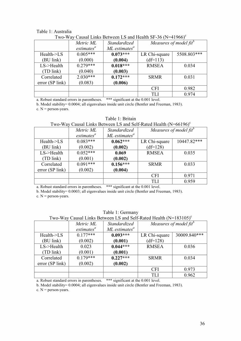
36

Table 1: Australia Two-Way Causal Links Between LS and Health SF-36 (N=41966)c

Metric ML estimatesa

Standardized ML estimatesa

Measures of model fitb

Health->LS (BU link)

0.005*** (0.000)

0.073*** (0.004)

LR Chi-square (df=113)

5508.803***

LS->Health (TD link)

0.279*** (0.040)

0.018*** (0.003)

RMSEA 0.034

Correlated error (SP link)

2.030*** (0.083)

0.172*** (0.006)

SRMR 0.031

CFI 0.982 TLI 0.974

a. Robust standard errors in parentheses. *** significant at the 0.001 level. b. Model stability= 0.0004; all eigenvalues inside unit circle (Bentler and Freeman, 1983). c. N = person-years.

Table 1: Britain Two-Way Causal Links Between LS and Self-Rated Health (N=66196)c Metric ML

estimatesa Standardized ML estimatesa

Measures of model fitb

Health->LS (BU link)

0.083*** (0.002)

0.062*** (0.002)

LR Chi-square (df=128)

10447.82***

LS->Health (TD link)

0.052*** (0.001)

0.069 (0.002)

RMSEA 0.035

Correlated error (SP link)

0.091*** (0.002)

0.156*** (0.004)

SRMR 0.033

CFI 0.971 TLI 0.959

a. Robust standard errors in parentheses. *** significant at the 0.001 level. b. Model stability= 0.0003; all eigenvalues inside unit circle (Bentler and Freeman, 1983). c. N = person-years.

Table 1: Germany Two-Way Causal Links Between LS and Self-Rated Health (N=183105)c Metric ML

estimatesa Standardized ML estimatesa

Measures of model fitb

Health->LS (BU link)

0.177*** (0.002)

0.093*** (0.001)

LR Chi-square (df=128)

30009.840***

LS->Health (TD link)

0.023 (0.001)

0.044*** (0.001)

RMSEA 0.036

Correlated error (SP link)

0.179*** (0.002)

0.227*** (0.002)

SRMR 0.034

CFI 0.973 TLI 0.962

a. Robust standard errors in parentheses. *** significant at the 0.001 level. b. Model stability= 0.0004; all eigenvalues inside unit circle (Bentler and Freeman, 1983). c. N = person-years.

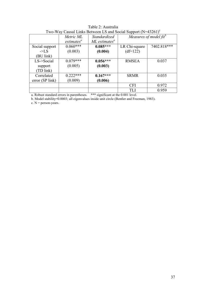
37

Table 2: Australia Two-Way Causal Links Between LS and Social Support (N=43261)c

Metric ML estimatesa

Standardized ML estimatesa

Measures of model fitb

Social support ->LS

(BU link)

0.060*** (0.003)

0.085*** (0.004)

LR Chi-square (df=122)

7402.818***

LS->Social support

(TD link)

0.079*** (0.005)

0.056*** (0.003)

RMSEA 0.037

Correlated error (SP link)

0.222*** (0.009)

0.167*** (0.006)

SRMR 0.035

CFI 0.972 TLI 0.959

a. Robust standard errors in parentheses. *** significant at the 0.001 level. b. Model stability=0.0003; all eigenvalues inside unit circle (Bentler and Freeman, 1983). c. N = person-years.

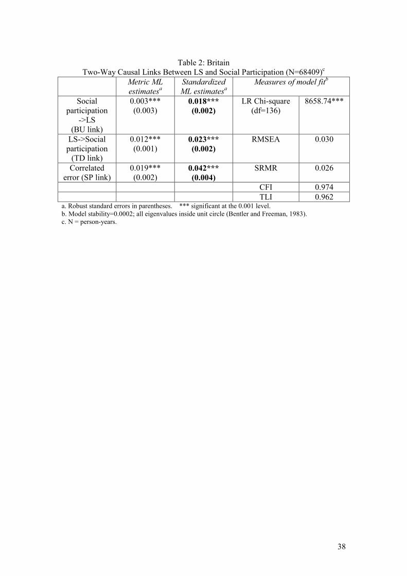
38

Table 2: Britain

Two-Way Causal Links Between LS and Social Participation (N=68409)c Metric ML

estimatesa Standardized ML estimatesa

Measures of model fitb

Social participation

->LS (BU link)

0.003*** (0.003)

0.018*** (0.002)

LR Chi-square (df=136)

8658.74***

LS->Social participation

(TD link)

0.012*** (0.001)

0.023*** (0.002)

RMSEA 0.030

Correlated error (SP link)

0.019*** (0.002)

0.042*** (0.004)

SRMR 0.026

CFI 0.974 TLI 0.962

a. Robust standard errors in parentheses. *** significant at the 0.001 level. b. Model stability=0.0002; all eigenvalues inside unit circle (Bentler and Freeman, 1983). c. N = person-years.

39

Table 2: Germany Two-Way Causal Links Between LS and Social Participation (N=182467)c

Metric ML estimatesa

Standardized ML estimatesa

Measures of model fitb

Social participation

->LS (BU link)

0.127*** (0.007

0.032*** (0.001)

LR Chi-square (df=122)

19034.395***

LS->Social participation

(TD link)

0.007*** (0.000)

0.027*** (0.001)

RMSEA 0.028

Correlated error (SP link)

0.010*** (0.001)

0.024*** (0.002)

SRMR 0.025

CFI 0.981 TLI 0.973

a. Robust standard errors in parentheses. *** significant at the 0.001 level. b. Model stability=0.0004; all eigenvalues inside unit circle (Bentler and Freeman, 1983). c. N = person-years.

40

Table 3: Australia Two-Way Causal Links Between LS and Exercise (N=43927)c

Metric ML estimatesa

Standardized ML estimatesa

Measures of model fitb

Exercise->LS (BU link)

0.028*** (0.003)

0.031*** (0.003)

LR Chi-square (df=120)

5167.150***

LS->Exercise (TD link)

0.017*** (0.004)

0.016*** (0.003)

RMSEA 0.031

Correlated error (SP link)

0.060*** (0.007)

0.050*** (0.006)

SRMR 0.030

CFI 0.974 TLI 0.961

a. Robust standard errors in parentheses. *** significant at the 0.001 level. b. Model stability=0.0002; all eigenvalues inside unit circle (Bentler and Freeman, 1983). c. N = person-years.

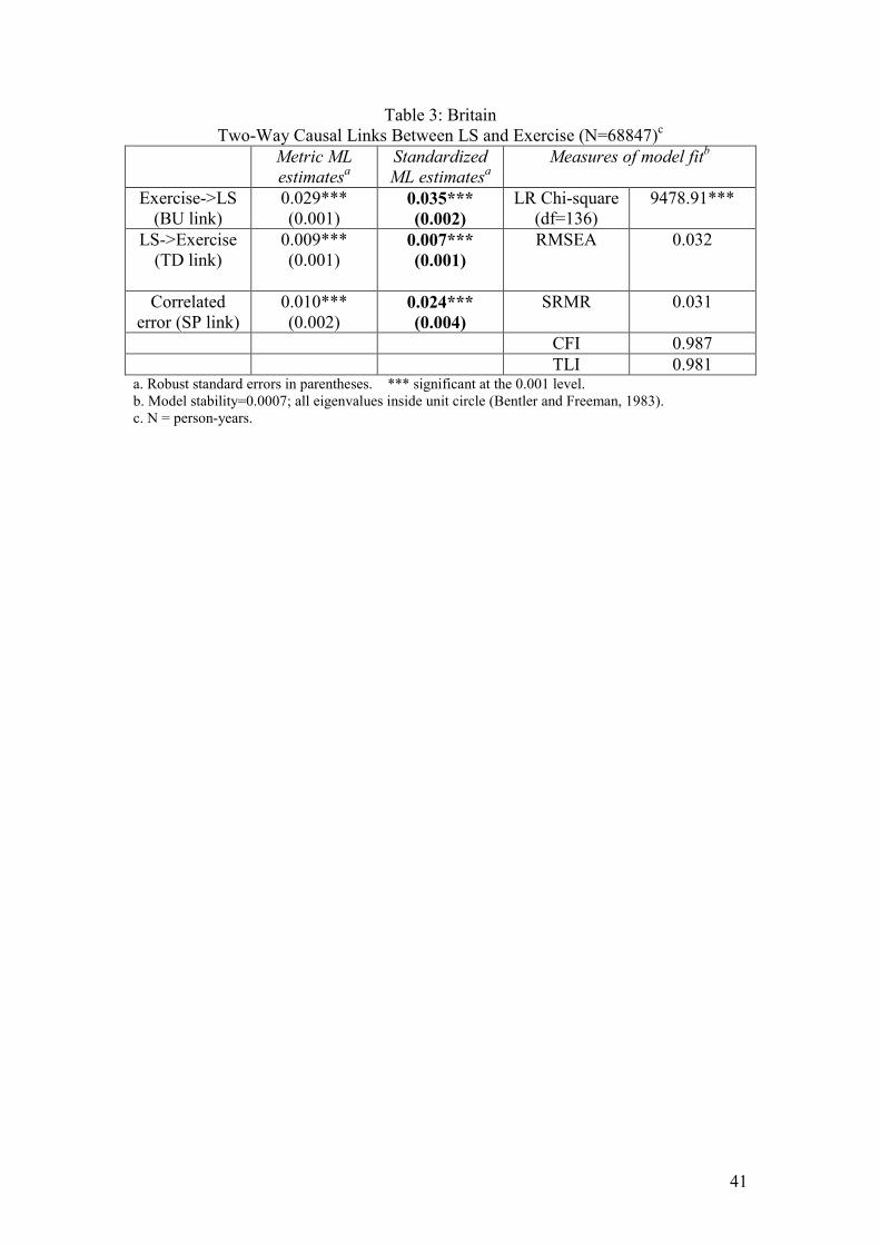
41

Table 3: Britain Two-Way Causal Links Between LS and Exercise (N=68847)c

Metric ML estimatesa

Standardized ML estimatesa

Measures of model fitb

Exercise->LS (BU link)

0.029*** (0.001)

0.035*** (0.002)

LR Chi-square (df=136)

9478.91***

LS->Exercise (TD link)

0.009*** (0.001)

0.007*** (0.001)

RMSEA 0.032

Correlated error (SP link)

0.010*** (0.002)

0.024*** (0.004)

SRMR 0.031

CFI 0.987 TLI 0.981

a. Robust standard errors in parentheses. *** significant at the 0.001 level. b. Model stability=0.0007; all eigenvalues inside unit circle (Bentler and Freeman, 1983). c. N = person-years.

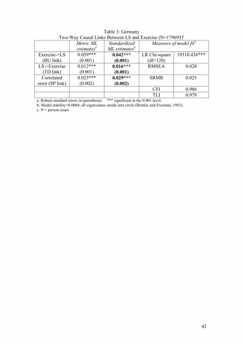
42

Table 3: Germany Two-Way Causal Links Between LS and Exercise (N=179693)c

Metric ML estimatesa

Standardized ML estimatesa

Measures of model fitb

Exercise->LS (BU link)

0.059*** (0.001)

0.042*** (0.001)

LR Chi-square (df=120)

19310.436***

LS->Exercise (TD link)

0.012*** (0.001)

0.016*** (0.001)

RMSEA 0.028

Correlated error (SP link)

0.025*** (0.002)

0.029*** (0.002)

SRMR 0.025

CFI 0.986 TLI 0.979

a. Robust standard errors in parentheses. *** significant at the 0.001 level. b. Model stability=0.0004; all eigenvalues inside unit circle (Bentler and Freeman, 1983). c. N = person-years.

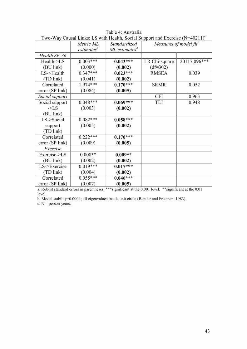
43

Table 4: Australia Two-Way Causal Links: LS with Health, Social Support and Exercise (N=40211)c

Metric ML estimatesa

Standardized ML estimatesa

Measures of model fitb

Health SF-36 Health->LS (BU link)

0.003*** (0.000)

0.043*** (0.002)

LR Chi-square (df=302)

20117.096***

LS->Health (TD link)

0.347*** (0.041)

0.023*** (0.002)

RMSEA 0.039

Correlated error (SP link)

1.974*** (0.084)

0.170*** (0.005)

SRMR 0.052

Social support CFI 0.963 Social support

->LS (BU link)

0.048*** (0.003)

0.069*** (0.002)

TLI 0.948

LS->Social support

(TD link)

0.082*** (0.005)

0.058*** (0.002)

Correlated error (SP link)

0.222*** (0.009)

0.170*** (0.005)

Exercise Exercise->LS

(BU link) 0.008** (0.002)

0.009** (0.002)

LS->Exercise (TD link)

0.019*** (0.004)

0.017*** (0.002)

Correlated error (SP link)

0.055*** (0.007)

0.046*** (0.005)

a. Robust standard errors in parentheses. ***significant at the 0.001 level. **significant at the 0.01 level. b. Model stability=0.0004; all eigenvalues inside unit circle (Bentler and Freeman, 1983). c. N = person-years.

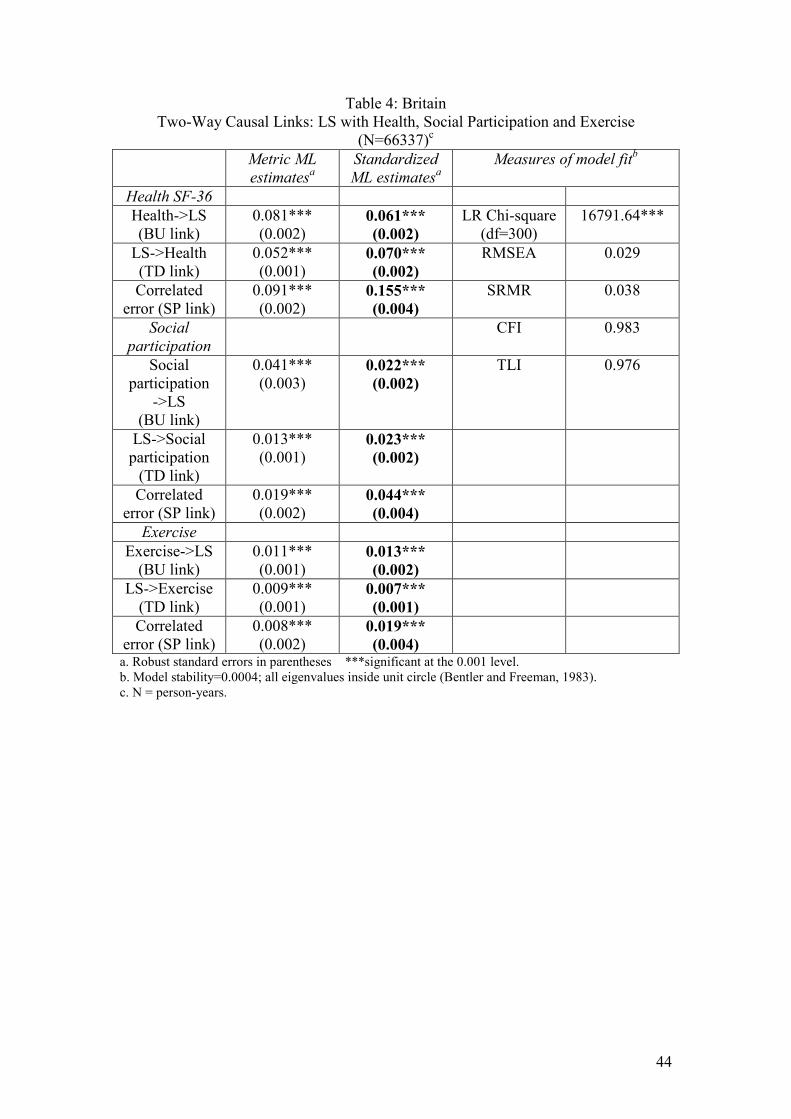
44

Table 4: Britain Two-Way Causal Links: LS with Health, Social Participation and Exercise

(N=66337)c Metric ML

estimatesa Standardized ML estimatesa

Measures of model fitb

Health SF-36 Health->LS (BU link)

0.081*** (0.002)

0.061*** (0.002)

LR Chi-square (df=300)

16791.64***

LS->Health (TD link)

0.052*** (0.001)

0.070*** (0.002)

RMSEA 0.029

Correlated error (SP link)

0.091*** (0.002)

0.155*** (0.004)

SRMR 0.038

Social participation

CFI 0.983

Social participation

->LS (BU link)

0.041*** (0.003)

0.022*** (0.002)

TLI 0.976

LS->Social participation

(TD link)

0.013*** (0.001)

0.023*** (0.002)

Correlated error (SP link)

0.019*** (0.002)

0.044*** (0.004)

Exercise Exercise->LS

(BU link) 0.011*** (0.001)

0.013*** (0.002)

LS->Exercise (TD link)

0.009*** (0.001)

0.007*** (0.001)

Correlated error (SP link)

0.008*** (0.002)

0.019*** (0.004)

a. Robust standard errors in parentheses ***significant at the 0.001 level. b. Model stability=0.0004; all eigenvalues inside unit circle (Bentler and Freeman, 1983). c. N = person-years.

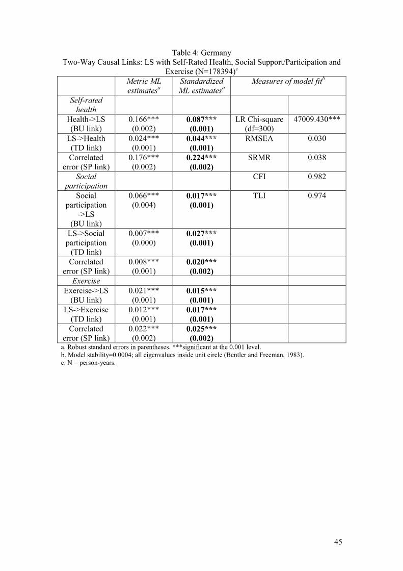
45

Table 4: Germany Two-Way Causal Links: LS with Self-Rated Health, Social Support/Participation and

Exercise (N=178394)c Metric ML

estimatesa Standardized ML estimatesa

Measures of model fitb

Self-rated health

Health->LS (BU link)

0.166*** (0.002)

0.087*** (0.001)

LR Chi-square (df=300)

47009.430***

LS->Health (TD link)

0.024*** (0.001)

0.044*** (0.001)

RMSEA 0.030

Correlated error (SP link)

0.176*** (0.002)

0.224*** (0.002)

SRMR 0.038

Social participation

CFI 0.982

Social participation

->LS (BU link)

0.066*** (0.004)

0.017*** (0.001)

TLI 0.974

LS->Social participation

(TD link)

0.007*** (0.000)

0.027*** (0.001)

Correlated error (SP link)

0.008*** (0.001)

0.020*** (0.002)

Exercise Exercise->LS

(BU link) 0.021*** (0.001)

0.015*** (0.001)

LS->Exercise (TD link)

0.012*** (0.001)

0.017*** (0.001)

Correlated error (SP link)

0.022*** (0.002)

0.025*** (0.002)

a. Robust standard errors in parentheses. ***significant at the 0.001 level. b. Model stability=0.0004; all eigenvalues inside unit circle (Bentler and Freeman, 1983). c. N = person-years.

46

Table 5: Australia Two-Way Causal Links: LS with Job Satisfaction and Satisfaction with Partner

(N=15848)c Metric ML

estimatesa Standardized ML estimatesa

Measures of model fitb

Job satisfaction

Job satis.->LS (BU link)

0.041*** (0.005)

0.055*** (0.004)

LR Chi-square (df=196)

1923.755***

LS->Job satis. (TD link)

0.163*** (0.011)

0.080*** (0.004)

RMSEA 0.024

Correlated error (SP link)

0.308*** (0.013)

0.288*** (0.007)

SRMR 0.031

Partner satisfaction

CFI 0.985

Partner satis. ->LS

(BU link)

0.051*** (0.004)

0.080*** (0.004)

TLI 0.978

LS->Partner satis. support

(TD link)

0.109*** (0.011)

0.067*** (0.004)

Correlated error (SP link)

0.228*** (0.014)

0.204*** (0.011)

a. Robust standard errors in parentheses. *** significant at the 0.001 level. b. Model stability=0.0002; all eigenvalues inside unit circle (Bentler and Freeman, 1983). c. N = person-years.

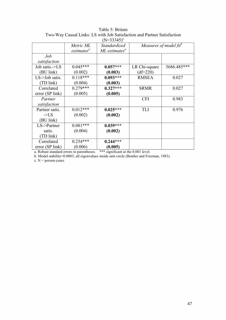
47

Table 5: Britain Two-Way Causal Links: LS with Job Satisfaction and Partner Satisfaction

(N=33345)c Metric ML

estimatesa Standardized ML estimatesa

Measures of model fitb

Job satisfaction

Job satis.->LS (BU link)

0.045*** (0.002)

0.057*** (0.003)

LR Chi-square (df=220)

5686.485***

LS->Job satis. (TD link)

0.118*** (0.004)

0.093*** (0.003)

RMSEA 0.027

Correlated error (SP link)

0.279*** (0.005)

0.327*** (0.005)

SRMR 0.027

Partner satisfaction

CFI 0.983

Partner satis. ->LS

(BU link)

0.012*** (0.002)

0.025*** (0.002)

TLI 0.976

LS->Partner satis.

(TD link)

0.081*** (0.004)

0.039*** (0.002)

Correlated error (SP link)

0.254*** (0.006)

0.244*** (0.005)

a. Robust standard errors in parentheses. *** significant at the 0.001 level. b. Model stability=0.0003; all eigenvalues inside unit circle (Bentler and Freeman, 1983). c. N = person-years.

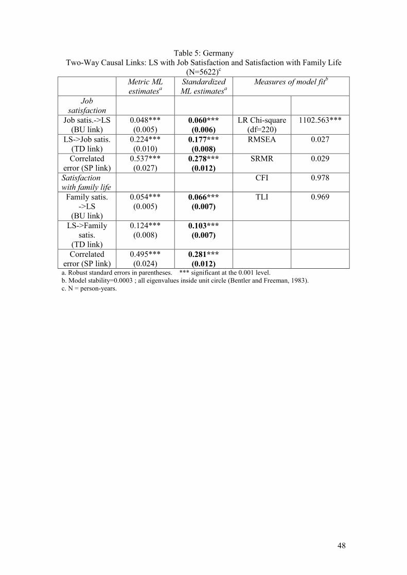
48

Table 5: Germany Two-Way Causal Links: LS with Job Satisfaction and Satisfaction with Family Life

(N=5622)c Metric ML

estimatesa Standardized ML estimatesa

Measures of model fitb

Job satisfaction

Job satis.->LS (BU link)

0.048*** (0.005)

0.060*** (0.006)

LR Chi-square (df=220)

1102.563***

LS->Job satis. (TD link)

0.224*** (0.010)

0.177*** (0.008)

RMSEA 0.027

Correlated error (SP link)

0.537*** (0.027)

0.278*** (0.012)

SRMR 0.029

Satisfaction with family life

CFI 0.978

Family satis. ->LS

(BU link)

0.054*** (0.005)

0.066*** (0.007)

TLI 0.969

LS->Family satis.

(TD link)

0.124*** (0.008)

0.103*** (0.007)

Correlated error (SP link)

0.495*** (0.024)

0.281*** (0.012)

a. Robust standard errors in parentheses. *** significant at the 0.001 level. b. Model stability=0.0003 ; all eigenvalues inside unit circle (Bentler and Freeman, 1983). c. N = person-years.

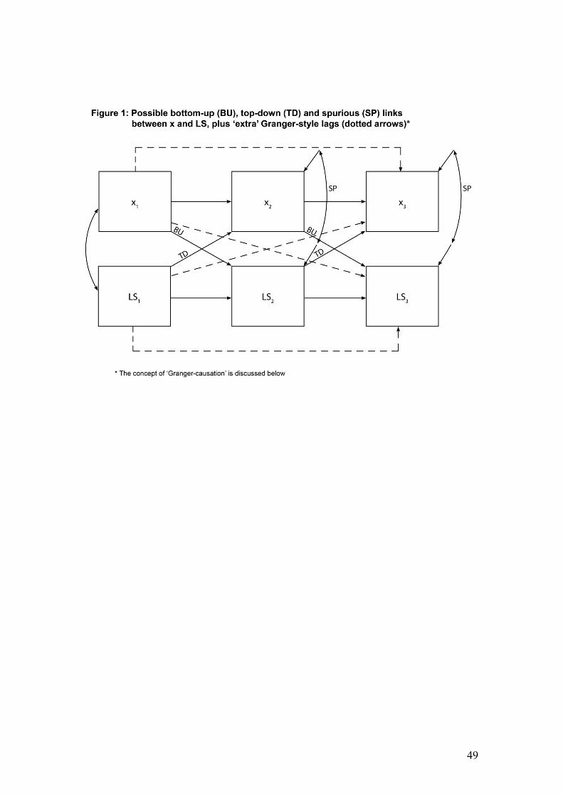
49

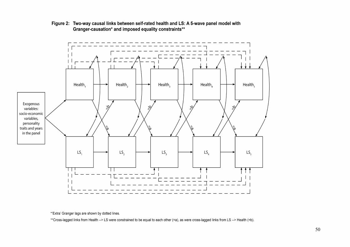
50