FIELD TESTING AND FINITE ELEMENT ANALYSIS FOR

EVALUATION OF RAILROAD BRIDGES

by

OZAN ETKIN KARA

A Thesis submitted to the

Graduate School – New Brunswick

Rutgers, The State University of New Jersey

in partial fulfillment of the requirements

for the degree of

Master of Science

Graduate Program in Civil and Environmental Engineering

written under the direction of

Dr. Hani H. Nassif

and approved by

_____________________________________

_____________________________________

_____________________________________

New Brunswick, New Jersey

January 2011

ii

ABSTRACT OF THE THESIS

FIELD TESTING AND FINITE ELEMENT ANALYSIS FOR

EVALUATION OF RAILROAD BRIDGES

by OZAN ETKIN KARA

Thesis Director:

Dr. Hani H. Nassif

ABSTRACT OF THE THESIS

Throughout the centuries, railroads have been the most important means of

transportation. The capacity of railroads should be increased with the booming economy.

In order to keep in step with an increased demand for freight, goods and services, New

Jersey Department of Transportation increased the capacity of existing railroads to be

able to increase the freight capacity. In New Jersey, a proposed increase of railcar weight

limits from 263,000 lb to 286,000 lb raised additional concerns for the passenger rail

systems since the bridges in the passenger rail system were not designed based on the

increased freight railcar weight. The effect of increased freight railcars on passenger rail

systems must be evaluated.

The impact of the proposed increase freight railcars on three rail road bridges in

New Jersey is investigated through the study presented herein. The AREMA

Specifications were utilized to estimate the load rating of the bridge. Moreover, strain

iii

transducers were implemented to the structural members of Bridge A, one of the selected

bridges, to collect strain measurements. Various measurements were performed to

measure the deflection in companion with the strain measurements by means of reflective

target tapes and Laser Doppler Vibration Unit. A total of 6 tests were performed with the

passenger railcars that NJ Transit provided the axle configuration and axle weights.

Additionally, a three dimensional finite element (FE) model was developed to

evaluate the behavior of three bridges under 286,000 lb railcar on a software program

ABAQUS (Version 6.8.1). The recorded deflection and strain readings from the strain

transducers and Laser Doppler Vibration Unit were utilized to calibrate the three

dimensional FE model. Results from AREMA evaluation procedure and those from FE

Model were compared.

A considerable difference arose between finite element analysis and simple beam

analysis based on AREMA Specifications. It was found out that the bridge has more

capacity to allow the increase of the freight railcar according to the finite element

analysis. A more conservative approach was adopted in AREMA Specifications.

iv

ACKNOWLEDGEMENTS

I would like thank my advisor Dr. Hani H. Nassif for his support throughout all

my study at Rutgers. It was an honor to work with him and have a state of his engineering

and life experience.

I would also like to thank Dr. Husam Najm and Dr. Kaan Ozbay for being in my

thesis committee and their valuable advices.

I would like to thank Rohit Patel and Michael Colville from Arora and Associates

for their help on my study.

I would like to thank Ed Konrath and Miki Krauker from NJDOT, David Dieck,

Charles Maliszewski and Paul Falkowski from NJ Transit for their suggestions and help.

I would like to thank my family for their infinite support and care during all

stages of my life.

Special thanks to Amy Deighan for her support and care at every stage in my life.

Special thanks to Ufuk Ates for his help at the early stages of my laboratory

experience. His friendship and support was really important.

Special thanks to Pasa Ahmet Iscanli, Arda Bakir, Pamir Erturk, Samed Atak,

Sinan Cankaya, Tayfun Kip, Turgut Karaman, Ekrem Gorkem, Aydin Sipit, Batuhan

Uslu, Gokhan Dogan, Caner Aksoy and Ali Fuat Aksoy for their infinite support

regardless of distance.

v

I would like to thank to Mehmet Yildiriouglu, Mert Kural, Aytug Pala, Erman

Ozguven, Kagan Aktas and Anil Yazici for their support and friendship during my study.

I would like to thank Tim Walkowich, Alex Rothstein and Parth Oza for their

help on my study. Special thanks to Dan Su for being a mentor for my study.

vi

TABLE OF CONTENTS

ABSTRACT OF THE THESIS .......................................................................................... ii

ACKNOWLEDGEMENTS ............................................................................................... iv

1 INTRODUCTION .......................................................................................................1

1.1 Problem Statement .............................................................................................1

1.2 Research Objectives and Scope .........................................................................4

1.3 The Selected Bridges .........................................................................................4

1.3.1 Bridge A .....................................................................................................4

1.3.2 Bridge B .....................................................................................................5

1.3.3 Bridge C .....................................................................................................5

1.4 Typical 286 Kips Railcars .................................................................................5

2 LITERATURE REVIEW ............................................................................................8

2.1 Introduction .......................................................................................................8

2.2 Bridge Load Rating Conducted by Other DOT .................................................9

2.2.1 Wisconsin DOT ..........................................................................................9

2.2.2 Pennsylvania DOT ...................................................................................14

2.3 Field Tests on Railroad Bridges ......................................................................18

2.3.1 Timber Trestle Bridges (Colorado State university) ................................18

2.3.2 Built-up Steel Girder Bridge (Rutgers University) ..................................21

vii

2.3.3 Built-up Steel Girder Bridge (University of Delaware) ...........................26

2.3.4 Built-up Truss Bridge (University of Connecticut)..................................28

2.4 Finite Element Modeling .................................................................................31

2.5 Summary ..........................................................................................................34

3 LOAD RATING USING AREMA SPECIFICATIONS ...........................................36

3.1 Rating of Existing Steel Bridge .......................................................................36

3.2 Load Rating of Bridge A .................................................................................41

3.2.1 286K Freight Railcar Ratings (Project Proposal Railcar) ........................46

3.2.1.1 Impact Factor ...................................................................................46

3.2.1.2 Moment Rating ................................................................................48

3.2.1.3 End Shear Rating .............................................................................50

3.2.1.4 286 Kip Equivalent Cooper-E Load Ratings ...................................51

4 INSTRUMENTATION AND FIELD TESTING ......................................................54

4.1 Structural Testing System ................................................................................54

4.2 Laser Doppler Vibrometer ...............................................................................57

4.3 Testing .............................................................................................................58

5 FINITE ELEMENT BRIDGE ANALYSIS ...............................................................72

5.1 Finite Element Model ......................................................................................72

5.1.1 Material Properties ...................................................................................73

viii

5.1.2 Element Selection and Analysis Procedure ..............................................74

5.1.3 Model Verifications..................................................................................75

6 COMPARISON OF RESULTS .................................................................................81

6.1 286Kip Rail Car Analysis ................................................................................81

6.2 E Cooper 80 Rail Car Analysis........................................................................86

6.3 Load Rating Calculations Using Finite Element Analysis ..............................87

6.3.1 Moment Rating .........................................................................................87

6.3.2 Shear Rating .............................................................................................89

6.4 286kip Rail Car and Field Data Comparison...................................................90

6.5 Load Rating Comparison between FE Model and Load Rating Calculations

Using AREMA Specifications .......................................................................................91

7 SUMMARY AND CONCLUSIONS ........................................................................94

7.1 Summary and Conclusions ..............................................................................94

7.2 Scope for Future Research ...............................................................................95

APPENDIX A – BRIDGE B .............................................................................................97

APPENDIX B – BRIDGE C............................................................................................100

APPENDIX C – quickBridge RESULTS ........................................................................103

REFERENCES ................................................................................................................115

ix

LIST OF FIGURES

Figure 1. View of Selected Bridge A for Field instrumentation and Testing. (Inspection

Cycle Report 3, 2005). .........................................................................................................3

Figure 2. General and Plan View of the Superstructure of Bridge B (Inspection Cycle

Report 3, 2002). ...................................................................................................................3

Figure 3. General Plan of Bridge C (Inspection Cycle Report 3, 2002). .............................4

Figure 4. 286 kips rail car (West Brook Associate and E80 Plus Constructors 2006) ......10

Figure 5. Defects in timber bridge (West Brook Associate and E80 Plus Constructors

2006) ..................................................................................................................................11

Figure 6. Differential settlement of steel bridge pier (West Brook Associate and E80 Plus

Constructors 2006) .............................................................................................................11

Figure 7. Rail car loadings (West Brook Associate and E80 Plus Constructors 2006) .....12

Figure 8. Railcar weight and dimension (Leighty III et al. 2004) .....................................16

Figure 9. Open-deck timber bridge; (a) Schematic drawing; (b) Stringer layout ..............18

Figure 10. Instrumentation on the bridge (Gutkowski et al. 2003) ....................................19

Figure 11. Test train (Gutkowski et al. 2003) ....................................................................20

Figure 12. Typical load position (Gutkowski et al. 2003) .................................................20

Figure 13. Tested Bridge (Nassif et al. 2002) ....................................................................22

x

Figure 14. Instrumentation locations (Nassif et al. 2002) ..................................................23

Figure 15. Installed sensors (Nassif et al. 2002) ................................................................23

Figure 16. Train positioned for static test (Nassif et al. 2002) ..........................................24

Figure 17. Typical deflection profile in Trough under train loading (Nassif et al. 2007) .25

Figure 18. Dynamic strain measured under moving train (Nassif et al. 2002 ...................25

Figure 19. Tested bridge (Chajes et al. 2001) ....................................................................26

Figure 20. Transducer locations (Chajes et al. 2001) ........................................................27

Figure 21. Typical strain time history data (Chajes et al. 2001) ........................................28

Figure 22. Tested railroad truss bridge (DelGrego 2008) ..................................................29

Figure 23. Stresses in diagonal members (DelGrego et al. 2008) .....................................30

Figure 24. Tied arch bridge (Malm and Andersson 2006).................................................32

Figure 25. Investigated arch bridge (Calcada et al. 2002) .................................................33

Figure 26. Finite element model of bridge for high speed train ........................................34

Figure 27. General View of Span 2 Superstructure and Underside of Girder 2 ................44

Figure 28. Cut-off Points on Girder 2 Span 2. ...................................................................45

Figure 29. Impact Load Configuration on the Floor Beams ..............................................47

Figure 30. Wireless Data Collection System, Bridge Diagnostics Inc. .............................55

xi

Figure 31. Technical Specications of Wi -Fi Data Collection System ..............................56

Figure 32. STS Strain Transducer Installed on a Bridge Superstructure Member ............57

Figure 33. Laser Doppler Vibrometer Measuring Deflections ..........................................58

Figure 34. General View of the Main Span and the Controlling Member for the Load

Rating (Center Girder), View from Google Maps. ............................................................58

Figure 35. Sensor Instrumentation and Test Equipment ....................................................59

Figure 36. Sensor Locations on the Plan View ..................................................................60

Figure 37. Sensor Locations at A-A Section (Midspan) ....................................................62

Figure 38. Sensor Locations at B-B Section (First Cut-off Point ......................................63

Figure 39. Location of Strain Gage Number 2 and 3 .........................................................63

Figure 40. Location of Strain Gages Number 5,6 and 7,8. ................................................64

Figure 41. Plan View and Direction of Case 2 and 3.........................................................64

Figure 42. Strain Data from Case 2, Sensors (a) 2045, (b) 2046, (c) 2049. (d) 2050. .......67

Figure 43. Strain Data from Case 4, Sensors (a) 2045, (b) 2046, (c) 2049. (d) 2050. .......68

Figure 44. Strain Data from Case 3, Sensors (a) 2045, (b) 2046, (c) 2049. (d) 2050 ........69

Figure 45. Strain Data from Case 5, Sensors (a) 2045, (b) 2046, (c) 2049. (d) 2050 ........70

Figure 46. Deflection Measurements, (a) Case 1, (b) Case 2. ...........................................71

Figure 47. FE Model ..........................................................................................................72

xii

Figure 48. Deflected Model with GP40-PH-2B Rail Car Loading. ...................................73

Figure 49. Connectors between Different Element Sets ....................................................74

Figure 50. Strain Data Comparison for Case 2, (a) Sensor 2049, (b) Sensor 2046. ..........76

Figure 51. Strain Data Comparison for Case 2, (a) Sensor 2050, (b) Sensor 2045. ..........77

Figure 52. Strain Data Comparison for Case 2, (a) Sensor 2487, (b) Sensor 2491. ..........77

Figure 53. Strain Data Comparison for Case 3, (a) Sensor 2045, (b) Sensor 2046. ..........78

Figure 54. Strain Data Comparison for Case 3, (a) Sensor 2049, (b) Sensor 2050. ..........78

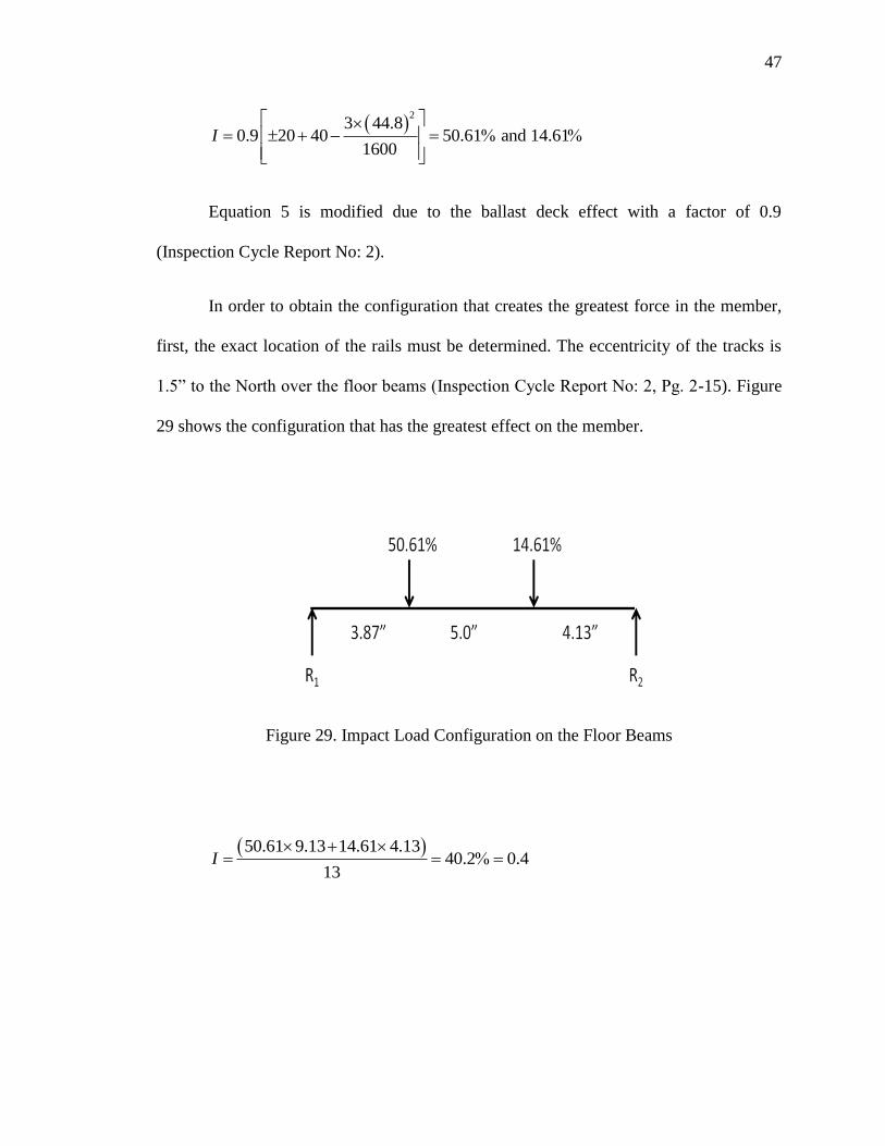
Figure 55. Strain Data Comparison for Case 3, (a) Sensor 2487, (b) Sensor 2490. ..........79

Figure 56. Strain Data Comparison for Case 3, (a) Sensor 2491, (b) Sensor 2493. ..........79

Figure 57. Deflection Data Comparison, (a) Case 1, (b) Case 2. ......................................80

Figure 58. Deflected Shape of FE Model due to Dead Load + Wind Load ......................82

Figure 59. Stress at, (a) First Cut-off Point, (b) Second Cut-off Point, (c) Third Cut-off

Point, (d) Midspan. ............................................................................................................83

Figure 60. Deflected Shape of the Finite Element Model under 286kip Rail Car Live

Load Configuration. ...........................................................................................................84

Figure 61. 286kip Rail Car Analysis, Deflection at the Midspan. .....................................84

Figure 62. 286kip Rail Car Analysis Results at the Location of Sensors , (a) 2487, (b)

2046, (c) 2491, (d) 2050. ...................................................................................................85

xiii

Figure 63. Deflected Shape of the Model due to Cooper E-80 Rail Car Loading .............86

Figure 64. Comparison between 286kip Rail Car Analysis, GP40-PH-2B Rail Car

Analysis and Field Data, (a) Midspan, (b) Second Cut-off Point, (c) Third cut-off Point,

(d) First Cut-off Point. .......................................................................................................90

Figure 65. Load Rating Results, Comparison between FEM and Simple Analysis ..........93

Figure 66. Bridge B – Finite Element Model ....................................................................99

Figure 67. Bridge C – Finite Element Model ..................................................................102

xiv

LIST OF TABLES

Table 1. 286-Kip Railcar Diagrams .....................................................................................7

Table 2. Timber bridge rating results (West Brook Associate and E80 Plus Constructors

2006) ..................................................................................................................................13

Table 3. Steel and concrete bridge rating results (West Brook Associate and E80 Plus

Constructors 2006) .............................................................................................................13

Table 4. Bridge sample selected for evaluation (Leighty III et al. 2004) ..........................15

Table 5. Capacity/Load ration in percentage (Leighty III et al. 2004) ..............................17

Table 6. Train axle weight (Gutkowski et al. 2003) ..........................................................21

Table 7. Allowable Stresses for Normal Rating (AREMA Manual 2010, Table 15-1-11,

Pg. 15-1-40) .......................................................................................................................39

Table 8. Allowable Stresses for Maximum Rating (AREMA Manual 2010, Table 15-7-1,

Pg. 15-7-19), y yK=F , where F is the allowable stress. (AREMA 2010, Pg. 15-7-18). .....40

Table 9. Live Load due to E-Cooper 80 Railcar & Section Capacity and Allowable

Stresses ...............................................................................................................................42

Table 10. Necessary Moments for Bridge A Load Rating.................................................48

Table 11. Necessary Shear Forces to Calculate End Shear Rating ....................................50

Table 12. Number of Sensors and Reflector Gages at Bridge A. ......................................60

xv

Table 13. Sensor ID Numbers and Locations ....................................................................61

Table 14. Information about the Tested Trains. .................................................................65

Table 15. Types and Configurations of Tested Rail Cars. .................................................66

Table 16. Laser Doppler Vibrometer, Location of Deflection Measurements ..................71

Table 17. Dead Load and Wind Load. ...............................................................................82

Table 18. 286kip Rail Car Analysis Results. .....................................................................82

Table 19. Cooper E-80 Analysis Results ...........................................................................86

Table 20. 286kip Rail Car Analysis Results, Shear Forces ...............................................89

Table 21. Normal Load Rating Comparison between FE Model Results and Simple Beam

Analysis Results at First Cut-off Point and Second Cut-off Point.....................................91

Table 22. Normal Load Rating Comparison between FE Model Results and Simple Beam

Analysis Results at First Cut-off Point and Second Cut-off Point.....................................92

Table 23. Maximum Load Rating Comparison between FE Model Results and Simple

Beam Analysis Results at First Cut-off Point and Second Cut-off Point. .........................92

Table 24. Maximum Load Rating Comparison between FE Model Results and Simple

Beam Analysis Results at First Cut-off Point and Second Cut-off Point. .........................93

Table 25. 286K Rail Car Live Loads Effecting on Girder 8, Midspan. .............................97

Table 26. Section Properties and Allowable Stresses for Midspan Girder 8. ....................98

xvi

Table 27. Comparison between FE Model and Simple Beam Analysis ............................99

Table 28. 286K Rail Car Live Loads Effecting on Member L4-L8 Span 13, Midspan. .100

Table 29. Section Properties and Allowable Stresses for Member L4-L8 Span 13,

Midspan............................................................................................................................101

Table 30. Comparison between FE Model and Simple Beam Analysis ..........................102

1

CHAPTER I

INTRODUCTION

1 INTRODUCTION

1.1 Problem Statement

The overall growth in the economy and population in the United States led to a

significant expansion of railroad traffic levels by the late 1990s. The freight railroad

system facilitates large volume of freight movement cost-effectively. The railroad system

is obviously important because the other alternative transportation methods, such as

vehicles and trucks, cause concerns about congestion, air quality, and safety. Moreover,

the cost to build and maintain new infrastructure and equipment is extremely high. Many

railroad bridges were built before World War II approaching their design lives, and

freight railcars, in many cases, use passenger rail systems to reduce maintenance cost.

In New Jersey freight railcars travel over many passenger rail systems. Recent

increase of railcar weight limits from 263,000 lb to 286,000 lb raised additional concerns

for the passenger rail systems since the bridges in the passenger rail system were not

designed based on the increased railcar weight. Impact of the railcar weight on those

bridges should be evaluated first to allow the use of passenger lines for the freight travels.

In this study, the impact of the increased railcar weight was investigated on the

bridges located in New Jersey. The research approach adopted by the RIME team is

aiming at evaluating current load-carrying capacity of various types of bridges and

2

providing recommendations for load rating, repair, and maintenance to allow 286,000-lb

railcar traffic on the passenger lines.

A detailed literature review was conducted to find similar previous research and

practices, followed by a review of inspection reports of all bridges. In cases where

inspection reports were not available or there was lack of information, current bridge

conditions and actual dimensions of the bridges were evaluated from field inspections.

Based on the field inspections, Bridges A and B (Figure 1) bridges on New Jersey’s rail

lines were selected and load-rated based on the current American Railway Engineering

and Maintenance-of-Way Association (AREMA) specifications as well as the analytical

studies. The selected bridges represent bridges with various structural systems and

material types. Finite element modeling was also adopted and the model was validated

using the data gathered in the field for more accurate assessment of the bridges and to

develop a methodology for evaluating and load-rating railroad bridges. The selected

bridges were instrumented and tested under live loads (moving railcars). Finally,

recommendations for load rating, maintenance, repair, and rehabilitation of the bridges

were provided for safe operation of the bridges on various New Jersey lines. The

recommendations will be applicable for other railroad bridges that support railcars with

the increased standard weight.

Briefly, this project addresses problems with the existing railroad bridges under

the increased railcar loading. Through this research, the RIME research team provides

guidelines for the inspection, maintenance, and load rating of the existing railroad bridges

as well as the cost-effective analysis of this change in the freight weight limits.

3

Figure 1. View of Selected Bridge A for Field instrumentation and Testing. (Inspection

Cycle Report 3, 2005).

Figure 2. General and Plan View of the Superstructure of Bridge B (Inspection Cycle

Report 3, 2002).

4

Figure 3. General Plan of Bridge C (Inspection Cycle Report 3, 2002).

1.2 Research Objectives and Scope

The main objective of this study is to evaluate current conditions of various

railroad bridges, and load-rate the bridges according to AREMA provisions to allow

travels of 286-kip railcars. Field tests and detailed finite element analysis were conducted

for more accurate condition evaluation of the bridges. Based on the study of the selected

railway bridges, general guidelines for bridge inspection and maintenance are also

provided in this study.

1.3 The Selected Bridges

1.3.1 Bridge A

Bridge A is a two track, three spans, simply supported riveted steel through plate

Girder Bridge which 77.0’ in length and 15.0’ in width. Both tracks are active. The

ballasted desk is supported by a steel deck late on rolled steel floor beams which frame

onto three through girders. The abutments and wing walls are plain concrete and the pier

column bents are built-up steel columns that are fully encased in concrete. The bridge

was built in 1930.

5

1.3.2 Bridge B

Bridge B is a four span, open deck, riveted deck plate girder. The bridge is

supported by one stone masonry abutment, one concrete abutment and 3 concrete piers.

The bridge carries two active tracks which are supported by Girders 5 through G8. The

bridge was built in 1902.

1.3.3 Bridge C

Bridge C is a seventeen span structure comprising through truss, bascule span and

deck girder approach spans. It has two active tracks. The bridge was built in 1911.

1.4 Typical 286 Kips Railcars

The basis of this study is to evaluate the live load effect on the selected bridges

due to various 286 kip railcars. Other than the project proposal car, five different 286 kip

railcars were investigated in terms of their live load effect on the bridges. Table 1 shows

the diagrams of 286 kip railcars.

Railcar diagrams through Number 2 to 4 were taken from the web page of

FreightCar America, Inc. The reasoning behind selecting those three railcars is due to the

fact that railcars with closer axle spacing provide conservative values needed. Railcars

Number 2, 3 and 4 have the shortest axle distances amongst the railcars available in the

FreightCar America catalogue.

The railcar diagram Number 5 is taken from a study of Wisconsin Department of

Transportation on which “Impact of Railcar Weight Change on Bridges of the State of

Wisconsin Owned Railroad System’.

6

The last railcar diagram is represented as a model railcar to develop a program

that will provide a consistent methodology for evaluating the timber bridge inventory.

This study was performed by John Horney, P.E. and presented in American Short Line

and Regional Railroad Association’s AREMA Conference in 2003, Chicago, IL.

7

Table 1. 286-Kip Railcar Diagrams

Car Type

Loading Diagram

1) Project Proposal

Railcar

2) Ore Hopper Railcar

(FreightCarAmerica)

3) Aggregate Railcar

(FreightCarAmerica)

4) Ballast Railcar

(FreightCarAmerica

)

5)WSOR Railcar

6) AREMA

Conference Railcar

2003

8

CHAPTER II

LITERATURE REVIEW

2 LITERATURE REVIEW

2.1 Introduction

In New Jersey freight railcars travel over many passenger rail systems. Recent

increase of railcar weight from 263,000 lb to 286,000 lb raised additional concerns for the

passenger rail systems since the bridges in the passenger rail system were not designed

based on the increased railcar weight. To increase the railcar weight, the 31 bridges on

the line between Oak Island rail yard and Metuchen need to be inspected and load-rated

to allow the 286,000-lb freight car travels. It is also required to provide maintenance,

repair, and retrofit recommendations to facilitate the heavier railcars.

As a first step of the project, previous research studies and practices were

reviewed in this study. Similar studies were already conducted by other transportation

agencies (West Brook Associate and E80 Plus Constructors 2006, Leighty III et al. 2004).

Wisconsin DOT and Pennsylvania DOT recognized the problem of the load-carrying

capacities of existing railroad bridges. They conducted bridge inspection, load rating, and

structural evaluations for the existing railroad bridges.

Field tests of the railroad bridges were conducted in many research studies

(Gutkowski, et al. 2003, Nassif et al. 2002, Chajes et al. 2001). Due to deterioration,

complex geometry, unexpected restraints, effects of non-structural elements, repair, and

9

modifications, the behavior of the railroad bridge under train loading can be different

from the intended behavior at the time of design and construction. Field tests sometimes

provide engineers with better understanding of the bridge behavior and load rating.

Information regarding test methods, instrumentation, and test setup was gathered in this

study to obtain better data from the possible bridge testing.

Due to the economical and practical limit, field tests cannot be conducted for all

the bridges. Finite element analysis method can be adopted for accurate load rating of the

bridge. Previous research studies on finite element modeling of the railroad bridges were

reviewed to build accurate bridge models.

Brief descriptions of load rating and strengthening methods of concrete, steel,

timber bridges are also presented in this study. American Railway Engineering and

Maintenance-of-Way Association (AREMA) also provides methods for repair and

strengthening of existing railroad bridges (AREMA 2000).

2.2 Bridge Load Rating Conducted by Other DOT

2.2.1 Wisconsin DOT

Similar study was conducted on Wisconsin railroad system to determine the

impact of 286-kips railcars (Figure 4). The condition of older existing railroad bridges

was additional concerns for the bridges. The scope of the project covers evaluating of

current condition, determining their load carrying capacity, and making repair and retrofit

recommendations based on the investigations.

10

Figure 4. 286 kips rail car (West Brook Associate and E80 Plus Constructors 2006)

In the study, 26 sample bridges were selected on two rail lines operated by

Wisconsin & Southern Railroad Co. The selected bridges consisted of steel bridges,

concrete bridges, timber bridges, and combined timber-steel bridges. The sample bridges

were built between 1900 and 1965.

Current condition of the selected bridges was inspected by field engineers.

Recommendations for repair and priority lists were provided based on the on-site

inspection results. For timber bridges, a complete visual inspection was conducted for

both superstructure and substructure. Bridge members were hammer sounded to inspect

the conditions of the bridge members, and holes were drilled to investigate the internal

decay if necessary. For steel and concrete bridges, a visual inspection was conducted

first. Concrete structures suspecting deterioration were hammer sounded to evaluate the

deterioration.

The inspection results indicate a requirement of several years of maintenance on

timber bridges. Many defects in the timber bridges were observed, including caps,

stringers and deck timbers (Figure 5). For steel and concrete bridges, the conditions were

11

relatively good. However, the pier settlement was observed at one of the bridge, which

requires a significant amount of maintenance cost (Figure 6).

(a) Defective stringer (b) Pile settlement

Figure 5. Defects in timber bridge (West Brook Associate and E80 Plus Constructors

2006)

Figure 6. Differential settlement of steel bridge pier (West Brook Associate and E80 Plus

Constructors 2006)

Two rail car loadings, the Cooper E80 load and the 286 kip railcar load, were

used for the load rating. The two railcar loads used for the analysis are shown in Figure 7.

12

In addition to the two railcar loading, the equivalent Cooper E load for the 286 kip rail

car was also used for the load rating. The equivalent Cooper E load causes the same load

effect as a series of 286 railcar loads.

Figure 7. Rail car loadings (West Brook Associate and E80 Plus Constructors 2006)

Two rating levels, normal rating and maximum rating, were considered in the load

rating. The normal rating level is the rating level which the structure can carry for its

service life without damage in the structure. The maximum rating level is the rating level

which the structure can carry at infrequent interval. The maximum load level may begin

to deteriorate and reduce its service life.

Rating results of a few bridges are shown in Table 2 and Table 3. In the study, the

rating results of the timber bridges showed that many of them are not able to carry

13

sustained heavy weight railcar traffic. For steel and concrete bridges, most of them are

able to allow the 286 kips freight car.

Table 2. Timber bridge rating results (West Brook Associate and E80 Plus Constructors

2006)

Table 3. Steel and concrete bridge rating results (West Brook Associate and E80 Plus

Constructors 2006)

14

The evaluation of the 26 sample bridges in Wisconsin showed that a sizable

amount of maintenance and repair were required for the bridges to support the 286-kips

freight cars. The study estimated the repair and strengthening cost of the bridges over the

next five years, and the cost was about $25 million to upgrade the railroad bridges in

Wisconsin and owned by the Wisconsin & Southern CO. For the sample bridges, about

$3 million was required to allow the 286-kips rail freight car.

The study gave priority for the repair recommendations from 1st priority

(Emergency) to 5th priority (Regular Maintenance) to have the State allocate the budget

more efficiently. The study also recommended immediate inspection and rating of all

bridges in Wisconsin and a routine maintenance and inspection program. This may

enable to extend the service life of the current bridges.

2.2.2 Pennsylvania DOT

Pennsylvania State University (Leighty III et al. 2004) sponsored by the

Pennsylvania Department of Transportation investigated the impact of higher rail car

weight on the load carrying capacity of short-line railroads (SLRR). Out of 2,000 bridges

located in Pennsylvania short-line railroads, 1,174 bridges were under consideration, and

25 sample bridges were selected and evaluated based on field test results and the

American Railway Engineering Association (AREA) Specifications. Load ratings of five

bridges out of 25 bridges were not high enough to support the 286 kips rail car loading

safely. Bridge strengthening methods were recommended for the under-capacity bridges,

and the retrofit cost was also obtained from contractors. Based on the studies of 25

bridges, state-wide rail bridge retrofit cost was also estimated in the study, which is $8.5

million.

15

Through a combination of mail surveys, telephone interviews, and on-site visits,

data was gathered from each bridge. The data gathered included milepost location, bridge

type, length, construction material, construction data, bridge width, Gross Car Weight

(GCW) capacity, date inspected, description of physical condition, availability of bridge

plans. Information was gathered for total 1,174 SLRR bridges.

The main interest of the study was to evaluate the cost for bridge strengthening to

carry the 286 kips rail car. The variables and bridge characteristics affecting the cost

include construction material, bridge type, length, deck width, and age. Considering those

variables, 25 representative bridges were selected to estimate a statewide bridge

strengthening. The selected bridges consist of eight bridge types and four construction

materials as shown in Table 4

.

Table 4. Bridge sample selected for evaluation (Leighty III et al. 2004)

16

For the selected 25 bridges, field inspections were conducted to evaluate current

conditions of the bridge which can be used for the load rating. This includes section loss

of structural members, unrecorded repair, and damage. The field inspection results were,

then, used for load rating. The sample bridges were evaluated for five different loading,

which are Cooper loading, Alternative live load, 263 kips railcar, 286 kips railcar, and

315 kips railcar (Figure 8). The loadings were applied with standard impact factor

without a reduction corresponding to speed.

Figure 8. Railcar weight and dimension (Leighty III et al. 2004)

17

In the study, evaluation results were reported as the percentage ratio of allowable

resistance to applied load. The results are listed in Table 5. As shown in the table, five

bridges out of the 25 sample bridges cannot carry the 286 kips railcar loading. Of the

sample bridges, 12 bridges meet E80 loading criteria. Note that many bridges can carry

315 kips railcar loading.

Table 5. Capacity/Load ration in percentage (Leighty III et al. 2004)

For the bridge which cannot carry the heavier 286 kips railcar and 315 kips

railcar, cost-effective methods were developed to strengthen the bridges. The

strengthening scheme includes post-tensioning floor-beam, alleviating soil pressure on

the wall of arch bridge, attaching steel channels to timber stringers, replacing deteriorated

timber members, and adding ties to steel truss members.

18

Construction cost of the developed strengthening techniques was estimated, and

the results were extrapolated to evaluate the repair and strengthening cost of the SLRR

bridges in Pennsylvania. Inspection, screening analysis, engineering analysis,

strengthening design costs were also added to the cost estimation. Detailed cost

estimation was made and the results were extrapolated to 2,000 bridges statewide. The

study concluded that the total cost to strengthen SLRR bridges n Pennsylvania for the

heavy axle railcars would be about $8.5 million.

2.3 Field Tests on Railroad Bridges

2.3.1 Timber Trestle Bridges (Colorado State university)

Colorado State University and Association of American Railroads (AAR)

conducted field tests of a timber trestle railroad bridge to determine the effects of

additional stringers on the stiffness of the bridge. A three-span timber bridge tested in the

study is shown Figure 9. The bridge is about 40 ft long, and main components were made

of creosote-treated Douglas fir timbers.

Figure 9. Open-deck timber bridge; (a) Schematic drawing; (b) Stringer layout

19

The bridge was instrumented with various sensors, which are displacement

transducers, extensometers, optical surveying equipment, and accelerometers. The

linearly variable differential transducers (LVDTs) were installed to measure relative

displacement between components and vertical displacement. Vertical displacements of

the bridge during the static tests were also measured with the optical survey equipment.

Accelerometers were used for the moving load testing. Figure 10 shows installed LVDTs

and extensometer for the tests.

Figure 10. Instrumentation on the bridge (Gutkowski et al. 2003)

Loading was applied to the bridge using the AAR’s track loading vehicle (TLV)

as shown in Figure 11. The TLV is able to apply concentrated loading to railroad track

using hydraulic actuators. By moving the TLV at various locations, the bridge was tested

under static loading. A typical TLV loading position is shown in Figure 12. Moving load

tests were also conducted while the test train passed over the bridge. The test train

consists of a locomotive, instrumentation car and TLV. The train axle weights are shown

in Table 6. In the study, sinusoidal loading using the TLV actuator was also applied to the

bridge.

20

Figure 11. Test train (Gutkowski et al. 2003)

Figure 12. Typical load position (Gutkowski et al. 2003)

21

Table 6. Train axle weight (Gutkowski et al. 2003)

Gutkowski et al. (2003) at Colorado State University also conducted similar tests

on part of a 31-span bridge, and a four-span bridge. Both of them are timber trestle

railroad bridges. Based on the test results and following analysis, the three span bridge

was strengthened by adding stringers in the bridge.

2.3.2 Built-up Steel Girder Bridge (Rutgers University)

Nassif et al. (2002) tested two steel girder bridges located in New Jersey. The

bridges have three spans with simply supported girders. The thru-girders are riveted built-

up girders, and overall length of the bridge is about 60 ft (Figure 13). A transverse trough

floor filled with stone ballast supports the rail lines. The field tests were conducted to

evaluate stresses and deflections of the bridges under passenger train loading and

compare with allowable stresses according to the current provisions.

Strain transducers and Linearly Variable Differential Transducers (LVDTs) were

installed to measure strains and displacements, respectively. A portable data acquisition

system was used to obtain data under the train loading. The instrumentation locations are

shown in Figure 14. The strain transducers and LVDTs were installed at south span

because the span had better accessibility than the other spans. Installed sensors are shown

22

in Figure 15. The strain transducers were installed to the steel flange with C-clamps or to

a custom-made steel plate attached to the bottom of the trough. The LVDTs were

installed on a temporary platform.

Figure 13. Tested Bridge (Nassif et al. 2002)

23

(a) LVDT locations in the bridge

(b) Strain transducer locations

Figure 14. Instrumentation locations (Nassif et al. 2002)

Figure 15. Installed sensors (Nassif et al. 2002)

24

Static tests were conducted by positioning a railcar at predetermined locations at

night time. A field engineer from Metro North communicated with an onboard engineer

to position the train at the locations (Figure 16). The train was stopped at each location

for 2 to 5 min. to obtain static test results. A typical deflection results from the static

loading is shown in Figure 17. Dynamic live load tests were also conducted under

multiple train passages with known axle weights. These dynamic tests were conducted to

evaluate the dynamic impact on the bridges. The trains were passed over the bridge at 10

mph and 70 mph.

The test results showed that the measured deflections are higher than the

calculated deflections with the full section properties (assuming no section loss). This

might be attributed to the section loss due to corrosion. Dynamic test results in the study

indicate that the dynamic impact factor for the bridge is lower than the AREMA

provisions. Figure 18 shows strain data measured at a girder, showing the difference in

the maximum strains between the two tests is not significant.

Figure 16. Train positioned for static test (Nassif et al. 2002)

25

Dynamic Trough Mid-Span Deflection

-0.25

-0.20

-0.15

-0.10

-0.05

0.00

0 1 2 3 4 5 6

Longitudinal Distance (ft)

Def

lect

ion

(in

.)

Genesis (2996) 70 mphGenesis (2903) 70 mphGenesis (2903) 10 mphGenesis (2901) 70 mph

South (LVDT 6)

Middle (LVDT 10)

North (LVDT 9)

Figure 17. Typical deflection profile in Trough under train loading (Nassif et al. 2007)

Girder Strain Profile

Train #2903 (Genesis) At Gage #5161

0 5 10 15 20 25 30 35

Time (sec.)

Str

ain

(me)

10 mph

70 mph

0

100

200

300

0

100

200

300

-100

-100

400

Max Strain = 291.1 me

Max Stress = 8.73 ksi

Max Strain = 278.0 me

Max Stress = 8.34 ksi

Figure 18. Dynamic strain measured under moving train (Nassif et al. 2002

26

2.3.3 Built-up Steel Girder Bridge (University of Delaware)

Chajes et al. (2001) at the University of Delaware conducted load tests and in-

service monitoring of a steel-girder railroad bridge. The bridge is located on the New

Jersey Transit line. The bridge is about 45-ft long, with simply supported girders (Figure

19). The bridge has two rails, but only one rail is used for service. Load rating of the

bridge is sufficiently low that the restriction on speed was applied on the bridge. To

evaluate the steel-girder bridge under the train loading, strain transducers were installed

on the bridge. Strain transducer locations and plan view of the bridge are shown in Figure

20.

Figure 19. Tested bridge (Chajes et al. 2001)

27

Figure 20. Transducer locations (Chajes et al. 2001)

The load test was conducted using the regularly scheduled transit train without

interrupting the train service. The locomotive weight was provided by NJ Transit

officials. A typical strain time history data measured under the moving passenger train is

shown in Figure 21. An in-service monitoring system was installed in the bridge after the

load test, and the stresses in the structural components were measured for a week. The

system automatically records time, peak strain, and strain transducer number when the

strains in the sensors are higher than a pre-specified strain limit. The test results showed

that the measured stresses were 15 percent of the computed stresses in the load rating,

indicating possible increase of current load rating of the bridge.

28

Figure 21. Typical strain time history data (Chajes et al. 2001)

2.3.4 Built-up Truss Bridge (University of Connecticut)

DelGrego et al. (2008) conducted tests on a truss railroad bridge with built-up

section members. Field monitoring under regularly scheduled train loading were

conducted to evaluate the structural behavior and live load distribution in the bridge. The

bridge tested by the team of the University of Connecticut was one of the typical large

truss bridge structures which were constructed with eye-bars, small angles, channels,

plates, lacing, and bars. The connections were made with large pins and rivets. The

monitoring of the bridge was conducted because of the lateral movement of the middepth

pins on the bridge. The experimental data provided an opportunity to compare the bridge

behavior under the train loading with the expected behavior in the original design which

was conducted more than 100 years ago.

29

The bridge tested has seven spans and the tested span is 210-ft long (Figure 22

(a)). A total 372 weldable strain gages were placed on different truss members, primarily

to tension members. Main interests of the tests were the load distribution in diagonal

members and load sharing in multiple eyebars (Figure 22 (b)), and the influence of floor

beam rotation on the adjacent truss members.

(a) Tested span (b) Multiple eyebars

Figure 22. Tested railroad truss bridge (DelGrego 2008)

Tests were conducted and data were collected for 16 different trains. A typical strain data

obtained during the tests is shown in Figure 23 which is for diagonal members. In the

study, DelGrego et al (2008) emphasized a significant influence of aging on the load-

carrying ability of the century-old truss. The difference in behavior from the design

assumption was also noted in the study.

30

(a) Truss member layout

(b) Collected data

Figure 23. Stresses in diagonal members (DelGrego et al. 2008)

31

2.4 Finite Element Modeling

Railway bridges have relatively short span compared to the bridges for the truck

traffic. Many railroad bridges have been in service for a long time and are composed of

timbers and built-up truss, and riveted built-up sections. Due to the simple structural

systems, simple frame analysis was adopted in many previous research studies

(Gutkowski et al. 2001, Chajes et al. 2001, Nassif et al. 2002). Detailed finite element

analysis for railroad bridges can be found in studies on the dynamic interaction between

railcars and tracks (Majka and Hartnett 2009, Song et al. 2003).

Malm and Andersson (2006) investigated dynamic effects of train passages on a

tied arch bridge. The bridge investigated is 45m long and used for both passenger and

freight train traffic. The bridge consists of two hollow arches without ballast. The finite

element (FE) model shown in Figure 24 was developed using the general purpose finite

element program, ABAQUS. The developed model was used to compare the field test

results with the simulation results and better understand the bridge behavior under the

moving train loading. Dynamic characteristics and structural behavior of the bridge were

investigated with the model as well as the field tests.

(a) Investigated bridge

32

(b) Bridge FE model

Figure 24. Tied arch bridge (Malm and Andersson 2006)

At the University of Porto (Calcada et al. 2002), Portugal, an arch bridge used for

urban road traffic was evaluated for possible use of the light rail (Figure 25 (a)). A

detailed FE model was developed to evaluate interaction between the bridge and the

trains and dynamic amplification factors for the moving train loads. The model was built

using the beam element as shown in Figure 25(b) and the developed model was validated

with field test results. After the validation, numerical simulations were conducted to

evaluate structural behaviors under the rail traffic.

33

(a) Existing bridge

(b) 3-dimensionl finite element model

Figure 25. Investigated arch bridge (Calcada et al. 2002)

Song et al. (2003) investigated the interaction between the high-speed train and

the bridge, and the analysis results with the model were compared with test results

conducted on the bridge. The deck of the bridge was modeled with the shell element and

the track structures were modeled with the beam element. Spring elements were used to

34

model ballast (Figure 26). In the study, a high-speed train model was also developed to

investigate the interaction between the train and the bridge.

Figure 26. Finite element model of bridge for high speed train

These detailed finite element analysis is not considered to be adequate for

the load rating of the existing railroad bridges in New Jersey. The modeling technique of

the railroad bridges, however, can be adopted for the bridge load rating.

2.5 Summary

The needs for condition evaluation of existing railroad bridges have been

identified by other transportation agencies. Wisconsin DOT and Pennsylvania DOT

conducted research on the existing bridges to allow the 286-kip railcars. The research

results showed that many timber trestle bridges do not satisfy the load rating for the

increased railcar weight. Field investigation of the bridges indicated significant

maintenance needs over several years.

35

Field tests of railroad bridges have been conducted in many research agencies to

identify bridge behavior under moving train loading and to evaluate stresses in the

structural components under the loading. Strains, deflections, and accelerations in the

bridges were measured in many studies. Many field tests were conducted under normally

scheduled train loading, and some tests were conducted by stopping trains at

predetermined locations. To further evaluate the bridge behavior, finite element analysis

programs were used in many studies. Field test results were used to validate the

developed model, and parametric studies were conducted with the validated model.

Due to the large number of railroad bridges and economical reasons, it is not

practically possible to replace many structurally deficient bridges in short time period.

Thus, studies have been conducted to develop efficient repair and strengthening methods

for existing bridges. It is considered that the developed methods by other researchers can

be used for existing bridges in New Jersey.

36

CHAPTER III

LOAD RATING USING AREMA SPECIFICATIONS

3 LOAD RATING USING AREMA SPECIFICATIONS

The American Railway Engineering and Maintenance-of-Way

Association (AREMA) was founded October 1, 1997 by merging four industry-related

groups: the American Railway Bridge and Building Association, the American Railway

Engineering Association (AREA), the Roadmasters and Maintenance of Way

Association, and the Communications and Signal Division of the Association of

American Railroads. AREMA publishes Manual for Railway Engineering with updates

annually. The Railway Company and consultants use the manual’s recommendation as a

basis for railway design in the United States and Canada.

3.1 Rating of Existing Steel Bridge

The rating of the existing steel bridges in terms of carrying capacity shall be

determined by the computation of stresses based on authentic records of the design,

details, materials, workmanship and physical condition, including data obtained by

inspection (and tests if the records are not complete). If deemed advisable, field

determination of stresses shall be made and the results given due consideration in the

final assignment of the structure carrying capacity. For a specific service the location and

behavior under load shall be taken into account (AREMA 2010). Please note the rating of

the bridge should be controlled by its weakest member.

37

The existing steel bridges may be assigned two types of ratings: Normal rating

and Maximum rating. The rating or ratings assignment should be directed by the

Engineer. If both ratings were computed, the lesser will govern.

(1) Normal Rating:

For Normal rating, it considered the load level can be carried by the expected life

of the bridge. This rating could be computed with allowable reduced speed per Article

7.3.3.3, Chapter 15 for impact deduction. The speed selection shall be directed by the

Engineer. Allowable stresses for normal rating were specified in Section 1.4, Chapter 15

supplemented by Article 1.3.14.3, and Chapter 15. The Normal rating should include the

fatigue requirements of Article 7.3.4.2, Chapter 15 unless a remaining fatigue service life

is computed.

The rating factor (SLN) was computed using the following formula:

fS D E B SF

SLNL I CF

Equation 1

Where,

SLN = Service Load Normal Rating Factor,

fS = Permissible Stress due to the Dead Load,

E = Effect due to the Earth Pressure,

B = Effect due to Buoyancy,

SF = Effect due to Stream Flow Pressure,

38

L = Effect due to Live Load,

I = Effect due to Impact Load,

CF = Effect due to Centrifugal Force.

Please note if the rating needs to be expressed in terms of Cooper EM (E) Series,

the rating value shall be computed using Equation 2 with regards to Cooper EM3600

(E80) series. For other Cooper EM (E) Series, the rating value would be changed

accordingly:

Normal Rating = SLN 360 (SLN 80) Equation 2

Normal ratings are evaluated with design allowable stresses shown in Table 7.

(2) Maximum Rating

For the Maximum rating, it considered the load level can be carried at infrequent

intervals with any applicable speed restrictions. Table 8 presents the allowable stresses

for Maximum rating. Fatigue need not be considered in Maximum Rating.

This rating factor (SLM) shall be computed in accordance with the following

formula:

fS D E B SFSLM

L I CF

Equation 3

Where,

SLM = Service Load Maximum Rating Factor.

39

Please note if the rating needs to be expressed in terms of Cooper EM (E) Series,

the rating value shall be computed using Equation 4 with regards to Cooper EM3600

(E80) series. For other Cooper EM (E) Series, the rating value would be changed

accordingly:

Maximum Rating = SLM 360 (SLM 80) Equation 4

This rating may be increased if the speed of traffic reduced. A reduction of impact

as defined in Section 19.3.4, Chapter 8, AREMA Manual for Railway Engineering (2010)

can be used to recalculate the rating.

Table 7. Allowable Stresses for Normal Rating (AREMA Manual 2010, Table 15-

1-11, Pg. 15-1-40)

40

Table 8. Allowable Stresses for Maximum Rating (AREMA Manual 2010, Table 15-7-1,

Pg. 15-7-19), y yK=F , where F is the allowable stress. (AREMA 2010, Pg. 15-7-18).

41

3.2 Load Rating of Bridge A

The steel used in the determination of member capacity of Bridge A were

assumed to be fabricated from “Open Hearth Steel” in accordance with Inspection Cycle

Reports. The yield strength,YF for open-hearth steel was taken as 30 ksi from AREMA

2010 Specification 7.3.4.3.

In this study, effect due to live load of 286 kips railcar was determined by using

the quickBridge, Moment and Shear Envelopes V1.2 – 2001 (Prof. Noyan Turkkan,

Ecole de Genie/School of Eng., Universite de Moncton, Canada). quickBridge is an Excel

program which analysis and estimates the moment and shear envelopes of a bridge due to

a moving vehicle. Vehicles may have 2 to 20 axles and bridges 1 to 5 spans which have

the constant EI. Results can be obtained either in tabular or graphical forms.

42

Table 9. Live Load due to E-Cooper 80 Railcar & Section Capacity and Allowable

Stresses

Section 1 Section 2 Section 3 Section 4

Mid span x=14.4' x=11.0' x=8.65'

MLL-E80 (k-ft) 3094.5 2756.3 2392.8 2009.3

Normal Moment Rating E 64 E 62 E 58 E 52

Maximum Moment Rating E 102 E 98 E 92 E 84

Section Modulus in3

3420.9 2940.5 2408.6 1878.5

Fy NORMAL (ksi) 16.5 16.5 16.5 16.5

Fy MAXIMUM (ksi) 24 24 24 24

M Capacity-NORMAL (k-ft) 4703.7 4043.2 3311.8 2582.9

M Capacity-MAXIMUM (k-ft) 6841.8 5881 4817.2 3757

V Allowable-NORMAL (ksi) 10.5

V Allowable-MAXIMUM (ksi) 18

V Capacity-NORMAL (kips) 543.4

V Capacity-MAXIMUM (kips) 931.5

Shear Normal Rating

Shear Maximum Rating

LIVE LOAD DUE TO E80 RAILCAR and LOAD RATINGS & SECTION CAPACITY

AND ALLOWABLE STRESSES

Only one section is considered for Shear Rating

Shear Area is 51.75 in2

E 77

E 144

43

Load ratings and the live load effect due to E-Cooper 80 Railcar represented on

Table 9 were acquired from Inspection Cycle Report No: 1, 1994, Pg. 65-72, where the

section properties and dimensions were taken from Inspection Cycle Report No: 2, 2001,

Pg. 2-23.

The load rating calculations based on following assumptions:

1- Ratings are as per New Jersey Transit Corp. “Rating Existing Railroad Bridges”

(2000).

2- Assumed each Girder carries half of the load per adjacent track.

3- Ratings for moments are at point of maximum moment and at plate cut-off.

Ratings for shear are at supports.

4- Steel assumed to be fabricated from “Open Hearth Steel”.

5- Allowable stresses for Ratings are as per A.R.E.M.A article 7.3.4.3 and 1.41.

6- Overstress calculations are not included.

7- Fatigue ratings are not included.

Controlling superstructure member was designated as Girder 2- Span 2 (Figure

27) in Inspection Cycle Report No: 2, 2001. Span length is 44.8 feet.

44

GIRDER 2

Figure 27. General View of Span 2 Superstructure and Underside of Girder 2

Girder 2 is riveted plate girder which has three cover plates on top and bottom.

The angles on top and bottom are riveted to the web plate. It is 69” in depth and 15” in

width. The methodology covered in Inspection Life Cycle Reports simply applies load

rating checks and calculations to the cut-off points and the maximum moment point

(Figure 28).

45

Third Cut-Off PointFirst Cut-Off Point

Second Cut-Off Point

Figure 28. Cut-off Points on Girder 2 Span 2.

First cut-off point is at 8.65’ distance from the bearing, where second and third

cut-off points are at 11.0’ and 14.4’ distance consecutively.

Since, Girder 2 is in good condition, as-inspected ratings are equal to as-built

ratings. Therefore, following calculations are for both as-inspected and as-built

conditions.

46

3.2.1 286K Freight Railcar Ratings (Project Proposal Railcar)

3.2.1.1 Impact Factor

Impact load, due to the sum of vertical effects and rocking effect created by

passage of locomotives and train loads, is determined by taking a percentage of the live

load. It is applied vertically at top of each rail.

Impact load due to vertical effects for span length less than 80 feet is determined

by the formula below;

23Impact 40

1600

L Equation 5

Equation 5 shows the related formula to calculate the impact factor in accordance

with AREMA 2010 1.3.5.

On the other hand, impact load due to rocking effect, RE, is created by the

transfer of load from the wheels on one side of the railcar to the other side from periodic

lateral rocking of the equipment. RE is calculated as a vertical force couple, each being

20 percent of the wheel load without impact, acting downward on one rail and upward on

the other. The couple is oriented in a way that creates the greatest force in the member.

Therefore, Equation 5 can be modified as follows;

23I 40

1600

LRE

Where,

20RE Equation 6

47

2

3 44.80.9 20 40 50.61 and 14.61

1600I

Equation 5 is modified due to the ballast deck effect with a factor of 0.9

(Inspection Cycle Report No: 2).

In order to obtain the configuration that creates the greatest force in the member,

first, the exact location of the rails must be determined. The eccentricity of the tracks is

1.5” to the North over the floor beams (Inspection Cycle Report No: 2, Pg. 2-15). Figure

29 shows the configuration that has the greatest effect on the member.

Figure 29. Impact Load Configuration on the Floor Beams

50.61 9.13 14.61 4.1340.2 0.4

13I

48

3.2.1.2 Moment Rating

Moment rating due to 286 kip railcar is calculated by modifying the equations 1

and 3. After finding the rating factor, it is multiplied with 71.5 kips which is the

maximum axle weight of the Project Proposal Railcar to find out the member rating due

to 286 kip railcar.

The effect due to live load of 286k Project Proposal Railcar, LL 286kipM (Table 10)

was determined by using qBridge Excel Program. Table 10 also shows DLM and

WLM values taken from the Inspection Cycle Report No: 2, Pg. 2-23.

Table 10. Necessary Moments for Bridge A Load Rating

MOMENT (k-ft) Section 1 Section 2 Section 3 Section 4

Maximum Resisting Capacity, Mrm 6841.8 5881.1 4817.2 3757.0

Normal Resisting Capacity, Mrn 4703.7 4043.2 3311.8 2582.9

Dead Load, MDL 972.7 844.7 718.3 603.3

Wind Load, MWL 72.0 62.5 53.4 44.9

Live Load due to 286kip railcar 2338.1 2079.3 1761.7 1498.3

49

Section 1 (Maximum Moment Point)

Cap DL WL

Normal Moment

LL 286kip

4703.7 972.7 72 = 71.5 71.5 79.92

Impact 1 2338.1 1.40

M M MR

M

Cap DL WL

Maximum Moment

LL 286kip

6841.8 972.7 72 = 71.5 71.5 126.63

Impact 1 2338.1 1.40

M M MR

M

Section 2 ( 14.4'x )

Cap DL WL

Normal Moment

LL 286kip

4043.2 844.7 62.5 = 71.5 71.5 77.03

Impact 1 2079.3 1.40

M M MR

M

Cap DL WL

Maximum Moment

LL 286kip

5881.0 844.7 62.5 = 71.5 71.5 122.17

Impact 1 2079.3 1.40

M M MR

M

Section 3 ( 11.0'x )

Cap DL WL

Normal Moment

LL 286kip

3311.8 718.3 53.4 = 71.5 71.5 73.64

Impact 1 1761.7 1.40

M M MR

M

Cap DL WL

Maximum Moment

LL 286kip

4817.2 718.3 53.4 = 71.5 71.5 117.28

Impact 1 1761.7 1.40

M M MR

M

Section 4 ( 8.65'x )

Cap DL WL

Normal Moment

LL 286kip

2582.9 603.3 44.9 = 71.5 71.5 65.95

Impact 1 1498.3 1.40

M M MR

M

50

Cap DL WL

Maximum Moment

LL 286kip

3757.0 603.3 44.9 = 71.5 71.5 105.97

Impact 1 1498.3 1.40

M M MR

M

3.2.1.3 End Shear Rating

Ratings for shear were carried for supports. Basically, the maximum reaction at

the supports due to 286 kip railcar live loading is used for end shear rating calculations.

Table 11 shows the necessary shear forces to carry out the shear end rating

calculations. Shear due to dead load and wind load were taken from Inspection Cycle

Report No: 2, Pg. 2-23. And live load effect due to 286 kip railcar is calculated by using

qBridge Excel Program.

Table 11. Necessary Shear Forces to Calculate End Shear Rating

VDL (kips) 86.84

VWL (kips) 6.44

VLL-286 (kips) 242.20

VRM (kips) 931.50

VRN (kips) 543.40

Cap DL WL

Normal Shear

LL 286kip

543.4 86.84 6.44 = 71.5 71.5 94.91

Impact 1 242.2 1.40

V V VR

V

Cap DL WL

Maximum Shear

LL 286kip

931.5 86.84 6.44 = 71.5 71.5 176.75

Impact 1 242.2 1.40

V V VR

V

51

3.2.1.4 286 Kip Equivalent Cooper-E Load Ratings

Equivalent Cooper E load rating is a measure of equipment in terms of live load

effect on a bridge member. It is simply to find out the live load effect of a Cooper E

railcar that is the same with the equipment generates.

In order to be able to make a reliable comparison between the load capacity of a

bridge member and live load effect of a railcar, to compute equivalent Cooper E load

rating is a significant milestone of the study.

Section 1 (Maximum Moment Point)

First, the ratio between moments of 286 kips railcar and Cooper E-80;

286

80

2338.1 0.756

3094.5

LL ki p

LL E

MMoment Ratio

M

Then, multiply the ration with the heaviest axle load of Cooper E-80 railcar which

is 80 kips.

286 Kips Equivalent Cooper E Load = Moment Ratio 80 0.756 80 60.48

Section 2 ( 14.4'x )

286

80

2079.3 0.75

2756.3

LL ki p

LL E

MMoment Ratio

M

E 60

52

286 Kips Equivalent Cooper E Load = Moment Ratio 80 0.75 80 60.35

Section 3 ( 11.0'x )

286

80

1761.7 0.736

2392.8

LL ki p

LL E

MMoment Ratio

M

286 Kips Equivalent Cooper E Load = Moment Ratio 80 0.736 80 58.9

It is not uncommon to have different equivalent load ratings on the same girder. It

is due to the differences in the axle spacing and positioning of the rail cars at the different

points of output generation. It means the load ratings can be different from each other

depending where the cutoff point is. It is possible that one axle of the 286 kip car "falls

off" the bridge. In other words, it is on the approach and not loading the bridge.

Section 4 ( 8.65'x )

286

80

1498.3 0.75

2009.3

LL ki p

LL E

MMoment Ratio

M

E 60

E 58

53

286 Kips Equivalent Cooper E Load = Moment Ratio 80 0.75 80 60.0

Since Section 8.65’ is critical (lowest rating), it is necessary to check whether

speed reduction calculations is required or not;

The AREMA rating equation for speed restrictions (Equation 7) must be equal or

greater than 0.2. This agrees with the principle that impact is no longer reduced once the

speed of the train goes below 10 mph, which would give 0.2 when input into the

equation. Speed restrictions apply only to the maximum ratings.

20.8 601 0.2

2500

SR

Equation 7

E 60 < E 84

(Original Cooper E Maximum Load Rating Value taking from Inspection Cycle

No: 3, Page 3-7a.)

Therefore, speed reduction calculations are not necessary.

E 60

54

CHAPTER IV

INSTRUMENTATION AND FIELD TESTING

4 INSTRUMENTATION AND FIELD TESTING

A complete field testing program was performed to understand the behavior of the

Bridge A. The target bridge was monitored to determine the actual strain and deflection

for load rating calculations and improve accuracy of the analysis model. In the bridge

monitoring, Structural Testing System (STS) Sensors and Laser Doppler Vibrometer

(LDV) were utilized.

4.1 Structural Testing System

The Structural Testing System (STS) is a modular data acquisition system

manufactured by Bridge Diagnostics, Inc. (BDI) of Boulder, Colorado. The system

consists of a main processing unit that samples data, junction boxes, and strain

transducers. The strain transducers are mounted to structural elements with clamps or

bolted to epoxied tabs. Each sensor has a unique identification number and a microchip,

so the sensors can be identified easily in the system. The sensor calibration factors are

stored in the configuration files and applied automatically. Main components and the

technical specifications of the Wi-Fi system are shown in Figure 30 and Figure 31

respectively.

55

Figure 30. Wireless Data Collection System, Bridge Diagnostics Inc.

The test system consists of strain transducers, junction box, and the main STS unit.

Each test is assigned to an automatic file number and the test is initiated using a trigger

button called the clicker. Once the test is completed, the data can be downloaded from the

STS unit to a laptop computer. The STS data files contain basic test information such as

date, time, duration, sensor ID numbers, and the stress data in ASCII text format. Figure

32 shows a strain gages installed on the floor beam flange.

56

Figure 31. Technical Specications of Wi -Fi Data Collection System

( Source ; http://www.bridgetest.com/products/STS3-WiFi.pdf)

57

Figure 32. STS Strain Transducer Installed on a Bridge Superstructure Member

4.2 Laser Doppler Vibrometer

The Laser Doppler Vibrometer (LDV), shown in Figure 33, is a non-contact

sensor that measures displacement and velocity of a remote point. A change in the

distance between the laser head and the reflective target will produce a Doppler shift in

the light frequency that is decoded into displacement and velocity. The system is

composed of three parts: 1) the helium neon Class II laser head, 2) the decoder unit, and

3) the reflective target attached to the structure. The laser head is mounted to a tripod

that is positioned underneath the target. The reflective target, typically retro-reflective

tape, provides the strongest signal. The signal strength is read on a scale on the laser

head. The tripod is adjusted to maximize the signal prior to a test run.

58

Figure 33. Laser Doppler Vibrometer Measuring Deflections

4.3 Testing

The sensor instrumentation at this structure will be focused on the center girder on

Span #2 since this member rates the lowest due to loading from 2 adjacent tracks on the

ballast deck. The behavior of the center girder will be evaluated at the cut-off locations

and at mid span.

For the exterior girders, strain gage installation will not be possible since the

girders are encased in concrete and the girder flanges are not accessible.

Figure 34. General View of the Main Span and the Controlling Member for the Load

Rating (Center Girder), View from Google Maps.

59

Figure 35. Sensor Instrumentation and Test Equipment

On 18th of September 2010, Saturday Rutgers Research Team met with Arora

Associates and Paterson Police to instrument strain transducers and laser reflective tapes

on Bridge A. Instrumentation started at 9:30 AM and finished at 12:30 PM. The sensors

and reflective tapes were installed to the bridge by means of a bucket truck which was

provided by Arora Associates. Research Team have run several tests with the scheduled

passenger trains of NJTransit from Paterson to Hawthorne at 11:58 AM, 12:58 PM &

1:58 PM and from Hawthorne to Paterson at 12:39, 1:39 and 2:39 PM (Table 14). During

the first run at 11:58 AM, only Laser Doppler Unit measurement could be executed, on

the other hand, the other runs involve STS Strain Transducer strain measurements also.

Table 12 shows the number of gages and reflector tapes that installed to the bridge.

60

Table 12. Number of Sensors and Reflector Gages at Bridge A.

Type of Sensor Number of Sensors Remark

STS strain transducers 12

Every 4 STS sensors connect

to one junction box, and then

the 5 junction boxes will be a

series system connects to

main processing unit.

Reflector for Laser

Doppler Vibrometer 5

Monitor the deflection of

various location on Floor-

beam and Girder

14'-8" 44'-10" 14'-8"

13'

13'

G1

G2

G3G4

G5

G6 G9

G8

G7

2 4

3

7

A

A

8

1 6

B

B

5

1

2

3

45

FB(TYP)

(Span 1) (Span 2) (Span 3)

Strain Gages

Laser Reflectors

Connection Boxes

PIER

CAP

2& 3

1

4

5 & 6 7 & 8 9

12

11

10

Figure 36. Sensor Locations on the Plan View

Figure 36 shows the location of the strain gages and reflector tapes that were

instrumented on the members of Bridge A. Since the controlling member was found out

61

to be the center girder after reviewing the previous inspection reports, the focus of sensor

instrumentation was shifted to this member.

Notes for Figure 36:

1. B-B Section is at the first cut-off location. (8.65 feet from the support).

Reflectors 1, 2, and 3. Strain gages 1, 2, 3 and 4.

2. A-A Section is at the mid span section. Reflector 5, Strain gages 10, 11, and 12.

3. Strain gages 5 and 6 are at the second cut off location.(11 feet from the support)

4. Reflectors 4 and Strain gages 7 and 8 are at the third cut off location.(14 feet from

the support)

Table 13. Sensor ID Numbers and Locations

Sensor No. Sensor ID Number Sensor Location

1 2047 Floor Beam (First Cut-off Point, G2-G3)

2 2049 Girder 2, First Cut-off Point, First Plate

3 2050 Girder 2, First Cut-off Point, Second Plate

4 2042 Floor Beam (First Cut-off Point, G1-G2)

5 2045 Girder 2, Second Cut-off Point, Second Plate

6 2046 Girder 2, Second Cut-off Point, Third Plate

7 2491 Girder 2, Third Cut-off Point, Third Plate

8 2490 Girder 2, Third Cut-off Point, Fourth Plate

9 2493

Girder 2, between Midspan and Third Cut-

off

10 2487 Girder 2, Midspan

11 2488 Floor Beam (Midspan, G2-G3)

12 2484 Floor Beam (Midspan, G2-G1)

62

Table 13 shows the unique ID numbers of the STS Strain Transducers that been

utilized for instrumentation of Bridge A.

Figure 37 to Figure 40 illustrates the sensor layout in a detailed view. At every

cut-off point, two sensors were attached to both of the plates to understand the behavior

of the girder when the cross section is changing throughout the length. Figure 39 and

Figure 40 demonstrate the sensor configuration on the cut-off points.

13' 13'

73.88"

15"

A-A Section

G2 G3G1

7

68

5

Strain Gages

Laser Reflectors

1112

10

Figure 37. Sensor Locations at A-A Section (Midspan)

63

13' 13'

73.88"

15"

B-B Section

G2 G3G1

2

13

2

Strain Gages

Laser Reflectors

3 14

2 & 3

1

Figure 38. Sensor Locations at B-B Section (First Cut-off Point

5 @ 3"11.5" 5 @ 4.5 "3.5"2 ' - 0 1316

First Cover

PlateFirst Physical

Cut-Off Point

Second Cover

Plate

4.38 "

1.25 "

1 ' - 3"

A

A

Figure 39. Location of Strain Gage Number 2 and 3

64

Second Cover Plate

Second Physical

Cut-Off Point

4.38 "

1.25 "

4.38 "

1.25 "

Third Cover

Plate

Third Physical

Cut-Off Point

13 @ 3 "8 @ 2 34

A

A

Figure 40. Location of Strain Gages Number 5,6 and 7,8.

Case 2, 4 and 6 to Paterson

Case 1, 3 and 5 to Hawthorne

Figure 41. Plan View and Direction of Case 2 and 3.

65

Table 14. Information about the Tested Trains.

Train

No

Case

Number Direction Time

Unit

Number Type

Locomotive

Weight, lbs

Number

of Axes

Distance

Between

Truck

Centers

Axle

Spacing

Axle

Weight

lbs

Speed

mph

1715 1 Paterson -

Hawthorne

11:58

AM 4100

GP40-

PH-20 293650 4 37’3” 9’

73412.

5 31.6

76 2 Hawthorne -

Paterson

12:39

PM 4201

GP40-

PH-2B 284200 4 37’3” 9’ 71050 31.4

1717 3 Paterson -

Hawthorne

12:58

PM 4029

PL-

42AC 288000 4 42’4” 9’5” 72000 30.9

1716 4 Hawthorne -

Paterson

1:39

PM 4100

GP40P

H-20 293650 4 37’3” 9’

73412.

5 37.4

1719 5 Paterson -

Hawthorne

1:58

PM 4904

GP40F

H-2M 282500 4 37’3” 9’ 70625 31.4

1718 6 Hawthorne -

Paterson

2:39

PM 4029

PL-

42AC 288000 4 42’4” 9’5” 72000 33.4

66

Table 15. Types and Configurations of Tested Rail Cars.

Train Type Rail Car Configuration

GP40-PH-20

GP40-PH-2B

PL-42AC

GP40FH-2M

The information about the tested trains including the axle configuration, axle

weight and speed (Table 14 and Table 15) were provided by NJ Transit to the Rutgers

Research Team.

Figure 41 shows the direction of each Case that tested with related trains on Table

14 and Table 15.

67

The strain and deflection measurements taken from the same direction cases show

similar values. Figure 42 to Figure 45 show typical strain data obtained from the STS

Strain Transducers.

-20

0

20

40

60

80

100

0 2 4 6 8 10 12

Sensor 2045

Str

ain

(µ

)

Time (s)

-20

0

20

40

60

80

100

0 2 4 6 8 10 12

Sensor 2046

Str

ain

(µ

)Time (s)

-20

0

20

40

60

80

100

0 2 4 6 8 10 12

Sensor 2049

Str

ain

(µ

)

Time (s)

-20

0

20

40

60

80

100

0 2 4 6 8 10 12

Sensor 2050

Str

ain

(µ

)

Time (s)

(a) (b)

(c) (d)

Figure 42. Strain Data from Case 2, Sensors (a) 2045, (b) 2046, (c) 2049. (d) 2050.

68

-20

0

20

40

60

80

100

0 2 4 6 8 10 12

Sensor 2045

Str

ain

(µ

)

Time (s)

-20

0

20

40

60

80

100

0 2 4 6 8 10 12

Sensor 2046

Str

ain

(µ

)

Time (s)

-20

0

20

40

60

80

100

0 2 4 6 8 10 12

Sensor 2049

Str

ain

(µ

)

Time (s)

-20

0

20

40

60

80

100

0 2 4 6 8 10 12

Sensor 2050

Str

ain

(µ

)

Time (s)

(a) (b)

(c) (d)

Figure 43. Strain Data from Case 4, Sensors (a) 2045, (b) 2046, (c) 2049. (d) 2050.

69

-20

0

20

40

60

80

100

0 2 4 6 8 10 12

Sensor 2045

Str

ain

(µ

)

Time (s)

-20

0

20

40

60

80

100

0 2 4 6 8 10 12

Sensor 2046

Str

ain

(µ

)

Time (s)

-20

0

20

40

60

80

100

0 2 4 6 8 10 12

Sensor 2049

Str

ain

(µ

)

Time (s)

-20

0

20

40

60

80

100

0 2 4 6 8 10 12

Sensor 2050

Str

ain

(µ

)

Time (s)

(a) (b)

(c) (d)

Figure 44. Strain Data from Case 3, Sensors (a) 2045, (b) 2046, (c) 2049. (d) 2050

70

-20

0

20

40

60

80

100

0 2 4 6 8 10 12

Sensor 2045

Str

ain

(µ

)

Time (s)

-20

0

20

40

60

80

100

0 2 4 6 8 10 12

Sensor 2046

Str

ain

(µ

)

Time (s)

-20

0

20

40

60

80

100

0 2 4 6 8 10 12

Sensor 2049

Str

ain

(µ

)

Time (s)

-20

0

20

40

60

80

100

0 2 4 6 8 10 12

Sensor 2050

Str

ain

(µ

)

Time (s)

(a) (b)

(c) (d)

Figure 45. Strain Data from Case 5, Sensors (a) 2045, (b) 2046, (c) 2049. (d) 2050

71

Table 16. Laser Doppler Vibrometer, Location of Deflection Measurements

Case No Reflective Target No

1 5

2 5

3 4

4 4

5 3

6 2

0

0.01

0.02

0.03

0.04

0.05

0.06

0.07

0.08

0

0.005

0.01

0.015

0.02

0.025

0.03

0 2 4 6 8 10 12

Defle

ction (

cm

)

Defle

ctio

n (in

ch)

Time (s)

0

0.01

0.02

0.03

0.04

0.05

0.06

0.07

0.08

0

0.005

0.01

0.015

0.02

0.025

0.03

0 2 4 6 8 10 12

Defle

ction (

cm

)

Defle

ctio

n (in

ch)

Time (s)

(a) (b)

Figure 46. Deflection Measurements, (a) Case 1, (b) Case 2.

72

CHAPTER V

FINITE ELEMENT BRIDGE ANALYSIS

5 FINITE ELEMENT BRIDGE ANALYSIS

Rail Bridge A was modeled and analyzed in the finite element program

ABAQUS (Version 6.8.1) to simulate the structural behavior of Span 2. The ultimate

objective is to evaluate the load rating of the bridge under 286kip railcar loading. This

section illustrates the ABAQUS FE model of the target bridge.

5.1 Finite Element Model

A three-dimensional finite element model was adopted to point out the behavior

of the bridge under 286kip railcar loading. To create the FE model, various modeling

features were considered including element types, material behavior, boundary conditions

and interaction between the floor beams and steel girders.

STEEL

GIRDER

FLOOR

BEAM

WOOD-TIE

RAILS

Figure 47. FE Model

73

Figure 47 shows the FE model. The model consists of 4 different members.

Figure 47 illustrates the members; 1) Steel Girders, 2) Steel Floor Beams, 3) Wood-Ties

and 4) Steel Rails.

Figure 48. Deflected Model with GP40-PH-2B Rail Car Loading.

5.1.1 Material Properties

The modulus of elasticity of the steel girder, steel beams and rails, E, and

Poisson’s Ratio, s , is used as 29,000 ksi and 0.3, respectively. Since, the steel girders,

steel beams and rails are not expected to show inelastic behavior, therefore, steel material

behavior was not considered in inelastic behavior.

Material properties for Wood-Tie members such as modulus of elasticity, E, and

Poisson’s Ratio, s were considered as 1,600 ksi and 0.3, respectively.

74

5.1.2 Element Selection and Analysis Procedure

The Steel Girders were modeled by using a 4-node shell element (S4). Element

type S4 in ABAQUS is a fully integrated, finite membrane strain shell element.

Simpson’s Rule is used to calculate the cross-sectional behavior of the shell elements

(ABAQUS 2008).

A 2-node linear beam element (B31) was selected in the model to simulate the

steel Floor Beams, Rails and Wood Ties. Element type B31 is a first-order, shear

deformable beam elements, meaning that shear deformation as well as flexural

deformation can be accounted in the analysis (ABAQUS 2008).

One type of connector element was used in the analysis model. Connection type

JOIN which makes the position of one node the same with the other node was utilized to

idealized the pin connections. JOIN connectors were used to idealize the bold

connections between Steel Girders and Floor Beams.

JOIN Connectors between Rail and Wood – Tie Elements

JOIN Connectors between Wood-Tie and Floor Beam Elements

Figure 49. Connectors between Different Element Sets

75

JOIN connectors were used to simulate the ballast deck between the wood ties

and the floor beams (Figure 49). Every element of a Wood – Tie member was connected

to the Floor Beam members to distribute the load uniformly as the ballast deck distributes

in reality.

JOIN connectors were also utilized to connect the Rail Elements to the Wood tie

elements (Figure 49).

In the model, a set of point loads simulating a rail car was applied on the Rail

Elements. A multiple load case analysis was adopted to apply the rail car loading at

various nodes on both tracks of the target bridge.

The accuracy of the model can be verified with comparing the strain and

deflection results gathered from the finite element analysis and the obtained field test

data.

5.1.3 Model Verifications

Deflections and strains of the structural elements were recorded from the strain

transducers and Laser Doppler Unit as the test rail cars passing over the bridge span. The

found deflection and strain of the structural members under the rail car loading were

compared with the analysis results.

Figure 50 to Figure 52 show the comparison for Case 2, when the rail car travels

from Hawthorne to Paterson. The horizontal axis shows the location of the rail car front

axle from west (designated direction in Cycle Reports) support in the span. The same

analysis was carried out for Case 3 (Figure 53 to Figure 56) when the rail car trails from

76

Paterson to Hawthorne. The horizontal axis shows the location of the rail car front axle

from east (designated direction in Cycle Reports) support in the span. Analysis results

using ABAQUS reflect good prediction of the bridge behavior under the same rail car

loading.

Deflection of the bridge under the rail car loading was also compared with the

model results. Figure 57 show the deflection comparison between FE Model and field

data at the Midspan for both Case 1 and Case 2. The horizontal axis is the distance from

the supports in the traveling direction.

-10

0

10

20

30

40

50

0 5 10 15 20 25 30 35 40 45

EXP

FE MODEL

Str

ain

(µ

)

Distance from Support (ft)

-10

0

10

20

30

40

50

0 5 10 15 20 25 30 35 40 45

EXP

FE MODELS

train

(µ

)

Distance from Support (ft)

(a) (b)

-10

0

10

20

30

40

50

0 5 10 15 20 25 30 35 40 45

EXP

FE MODEL

Str

ain

(µ

)

Distance from Support (ft)

Figure 50. Strain Data Comparison for Case 2, (a) Sensor 2049, (b) Sensor 2046.

77

-10

0

10

20

30

40

50

0 5 10 15 20 25 30 35 40 45

EXP

FE MODEL

Str

ain

(µ

)

Distance from Support (ft)

-10

0

10

20

30

40

50

0 5 10 15 20 25 30 35 40 45

EXP

FE MODEL

Str

ain

(µ

)

Distance from Support (ft)

(a) (b)

-10

0

10

20

30

40

50

0 5 10 15 20 25 30 35 40 45

EXP

FE MODEL

Str

ain

(µ

)

Distance from Support (ft)

Figure 51. Strain Data Comparison for Case 2, (a) Sensor 2050, (b) Sensor 2045.

-10

0

10

20

30

40

50

0 5 10 15 20 25 30 35 40 45

EXP

FE MODEL

Str

ain

(µ

)

Distance from Support (ft)

(a) (b)

-10

0

10

20

30

40

50

0 5 10 15 20 25 30 35 40 45

EXP

FE MODEL

Str

ain

(µ

)

Distance from Support (ft)

Figure 52. Strain Data Comparison for Case 2, (a) Sensor 2487, (b) Sensor 2491.

78

-10

0

10

20

30

40

50

0 5 10 15 20 25 30 35 40 45

EXPFE MODEL

Str

ain

(µ

)

Distance from Support (ft)

(a) (b)

-10

0

10

20

30

40

50

0 5 10 15 20 25 30 35 40 45

EXP

FE MODEL

Str

ain

(µ

)

Distance from Support (ft)

Figure 53. Strain Data Comparison for Case 3, (a) Sensor 2045, (b) Sensor 2046.

-10

0

10

20

30

40

50

0 5 10 15 20 25 30 35 40 45

EXPFE MODEL

Str

ain

(µ

)

Distance from Support (ft)

-10

0

10

20

30

40

50

0 5 10 15 20 25 30 35 40 45

EXPFE MODEL

Str

ain

(µ

)

Distance from Support (ft)

(a) (b)

Figure 54. Strain Data Comparison for Case 3, (a) Sensor 2049, (b) Sensor 2050.

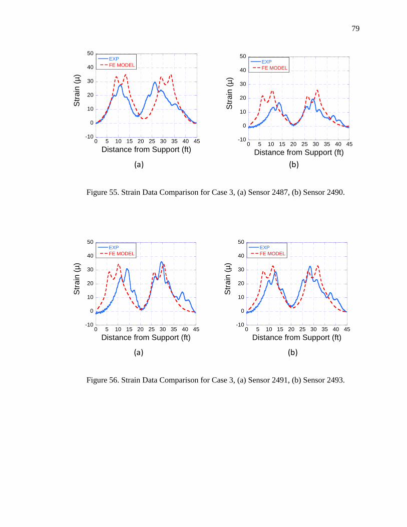
79

-10

0

10

20

30

40

50

0 5 10 15 20 25 30 35 40 45

EXP

FE MODEL

Str

ain

(µ

)

Distance from Support (ft)

-10

0

10

20

30

40

50

0 5 10 15 20 25 30 35 40 45

EXP

FE MODEL

Str

ain

(µ

)

Distance from Support (ft)

(a) (b)

Figure 55. Strain Data Comparison for Case 3, (a) Sensor 2487, (b) Sensor 2490.

-10

0

10

20

30

40

50

0 5 10 15 20 25 30 35 40 45

EXP

FE MODEL

Str

ain

(µ

)

Distance from Support (ft)

-10

0

10

20

30

40

50

0 5 10 15 20 25 30 35 40 45

EXP

FE MODEL

Str

ain

(µ

)

Distance from Support (ft)

(a) (b)

Figure 56. Strain Data Comparison for Case 3, (a) Sensor 2491, (b) Sensor 2493.

80

0

0.01

0.02

0.03

0.04

0.05

0 5 10 15 20 25 30 35 40 45

EXP

FE MODEL

Dis

pla

cem

ent

(inches)

Distance from Support (ft)

0

0.01

0.02

0.03

0.04

0.05

0 5 10 15 20 25 30 35 40 45

EXP

FE MODEL

Dis

pla

cem

ent

(inches)

Distance from Support (ft)

(a) (b)

Figure 57. Deflection Data Comparison, (a) Case 1, (b) Case 2.

The difference between the FE model analysis results and the field test results can

be addressed to the unexpected restraints at connections and supports. Possible small

dimension differences between the actual bridge sections and the FE model can be

attributed to the variation between the analysis results and the field test results. Another

reason of having that variation can be also addressed to idealization of load distribution

through the ballast deck. The connectors between Wood-Tie members and Floor Beam

members were modeled to distribute load applying on the Rail element, where, in reality,

the load is distributed to the floor beams and girders through the ballast deck. From the

comparison made, the developed analytical model displays good estimate for the actual

behavior of the target bridge under rail car loading.

81

CHAPTER VI

COMPARISON OF RESULTS

6 COMPARISON OF RESULTS

6.1 286Kip Rail Car Analysis

The Project Proposal Rail Car was selected to analyze for 286kip rail car analysis

case after having the model calibrated. Table 1 shows the configuration of the rail car.

The loading was considered two rail cars traveling on the direction Hawthorne to

Paterson consecutively. In order to input the necessary parameters to Equation 1, two

separate cases were analyzed on finite element model. The loading system of the first

case consists of live load effect due to the 286kip rail car. On the other hand, dead load

and wind load without any effect of live load was considered on the second case (Figure

58). Figure 61 shows how the model deflects at the Midspan. Figure 62 illustrates how

the model behaves under Project Proposal Rail Car in terms of stress and strain at cut-off

points and Midspan.

Dead Load and Wind Load are taken from Bridge Evaluation Survey Report,

Cycle 1.

82

Table 17. Dead Load and Wind Load.

Load Type Load, K/FT

G1, Dead Load 3.16

G2, Dead Load 3.47

G3, Dead Load 3.16

Wind Load 0.2

Table 18. 286kip Rail Car Analysis Results.

Midspan

Third

Cut-off

Point

Second

Cut-off

Point

First

Cut-off

Point

Max. Stress, ksi 1.70 1.62 1.43 0.98

Section Modulus, in3

3420.90 2940.5 2408.6 1878.5

Max. Moment due to

Live Load, k-ft 484 397 287 153

Moment due to Dead

Load + Wind Load, k-ft 328 168 165 54

Figure 58. Deflected Shape of FE Model due to Dead Load + Wind Load

83

-1000

-500

0

500

1000

1500

2000

0 10 20 30 40

Str

ess,

psi

Distance from Support, ft

-1000

-500

0

500

1000

1500

2000

0 10 20 30 40

Str

ess,

psi

Distance from Support, ft

-1000

-500

0

500

1000

1500

2000

0 10 20 30 40

Str

ess,

psi

Distance from Support, ft

-1000

-500

0

500

1000

1500

2000

0 10 20 30 40

Str

ess,

psi

Distance from Support, ft

(a) (b)

(c) (d)

Figure 59. Stress at, (a) First Cut-off Point, (b) Second Cut-off Point, (c) Third Cut-off

Point, (d) Midspan.

84

Figure 60. Deflected Shape of the Finite Element Model under 286kip Rail Car Live

Load Configuration.

0

0.01

0.02

0.03

0.04

0.05

0.06

0 10 20 30 40 50

286

Defle

ction

(in

ch)

Distance from Support (ft)

Figure 61. 286kip Rail Car Analysis, Deflection at the Midspan.

85

.

-10

0

10

20

30

40

50

60

-0.5

0

0.5

1

1.5

2

0 10 20 30 40 50

strain

stress

Str

ain

(µ

)

Stre

ss (k

si)

Distance from Support (ft)

-10

0

10

20

30

40

50

60

-0.5

0

0.5

1

1.5

2

0 10 20 30 40 50

strain

stress

Str

ain

(µ

)

Stre

ss (k

si)

Distance from Support (ft)

-10

0

10

20

30

40

50

60

-0.5

0

0.5

1

1.5

2

0 10 20 30 40 50

strain

stress

Str

ain

(µ

)

Stre

ss (k

si)

Distance from Support (ft)

-10

0

10

20

30

40

50

60

-0.5

0

0.5

1

1.5

2

0 10 20 30 40 50

strain

stress

Str

ain

(µ

)

Stre

ss (k

si)

Distance from Support (ft)

(a) (b)

(c) (d)

Figure 62. 286kip Rail Car Analysis Results at the Location of Sensors , (a) 2487, (b)

2046, (c) 2491, (d) 2050.

86

6.2 E Cooper 80 Rail Car Analysis

E Cooper -80 Rail Car was analyzed to rate the effect of 286kip rail car in terms

of E-Cooper Loading. Table 19 shows the found stresses and moments.

Table 19. Cooper E-80 Analysis Results

Midspan

Third

Cut-off

Point

Second

Cut-off

Point

First

Cut-off

Point

Max. Stress, ksi 2.22 2.04 1.83 1.24

Section Modulus, in3

3420.9 2940.5 2408.6 1878.5

Max. Moment due to

Live Load, k-ft 627 500 368 194

Figure 63. Deflected Shape of the Model due to Cooper E-80 Rail Car Loading

87

6.3 Load Rating Calculations Using Finite Element Analysis

6.3.1 Moment Rating

Section 1 (Maximum Moment Point)

Cap DL WL

Normal Moment

LL 286kip

4703.7 328 = 71.5 71.5 460

Impact 1 485 1.40

M M MR

M

Cap DL WL

Maximum Moment

LL 286kip

6841.8 328 = 71.5 71.5 685

Impact 1 485 1.40

M M MR

M

286

80

484.0 0.7719

627

LL ki p

LL E

MMoment Ratio

M

286 Kips Equivalent Cooper E Load = Moment Ratio 80 0.7719 80 61

Section 2 ( 14.4'x )

Cap DL WL

Normal Moment

LL 286kip

4043.2 168 = 71.5 71.5 498

Impact 1 397 1.40

M M MR

M

Cap DL WL

Maximum Moment

LL 286kip

5881.0 168 = 71.5 71.5 734

Impact 1 397 1.40

M M MR

M

286

80

397 0.794

500

LL ki p

LL E

MMoment Ratio

M

286 Kips Equivalent Cooper E Load = Moment Ratio 80 0.794 80 63

88

Section 3 ( 11.0'x )

Cap DL WL

Normal Moment

LL 286kip

3311.8 165 = 71.5 71.5 559

Impact 1 287.14 1.40

M M MR

M

Cap DL WL

Maximum Moment

LL 286kip

4817.2 165 = 71.5 71.5 827

Impact 1 287.14 1.40

M M MR

M

286

80

287 0.779

368

LL ki p

LL E

MMoment Ratio

M

286 Kips Equivalent Cooper E Load = Moment Ratio 80 0.79 80 62

Section 4 ( 8.65'x )

Cap DL WL

Normal Moment

LL 286kip

2582.9 53.68 = 71.5 71.5 844

Impact 1 153.04 1.40

M M MR

M

Cap DL WL

Maximum Moment

LL 286kip

3757.0 53.68 = 71.5 71.5 1235

Impact 1 153.04 1.40

M M MR

M

286

80

153 0.788

194

LL ki p

LL E

MMoment Ratio

M

286 Kips Equivalent Cooper E Load = Moment Ratio 80 0.788 80 63

89

6.3.2 Shear Rating

Table 20. 286kip Rail Car Analysis Results, Shear Forces

V DL + VWL 39.58 kips

V LL 61.7 kips

V Normal 543.4 kips

V Maximum 931.5 kips

Cap DL WL

Normal Shear

LL 286kip

543.4 39.58 = 71.5 71.5 417

Impact 1 61.7 1.40

V V VR

V

Cap DL WL

Maximum Shear

LL 286kip

931.5 39.58 = 71.5 71.5 738

Impact 1 61.7 1.40

V V VR

V

90

6.4 286kip Rail Car and Field Data Comparison

When the strain values in Figure 62 compares to the testing data obtained from

GP40-PH-2B Rail Car run, it can be said that the 286kip rail car analysis will show a

good prediction. Figure 64 shows the comparison between 286kip rail car analysis,

GP40-PH-2B Rail Car analysis and field test data.

-10

0

10

20

30

40

50

60

0 10 20 30 40 50

EXPFE MODEL286

Str

ain

(µ

)

Distance from Support (ft)

-10

0

10

20

30

40

50

60

0 10 20 30 40 50

EXPFE MODEL286

Str

ain

(µ

)

Distance from Support (ft)

-10

0

10

20

30

40

50

60

0 10 20 30 40 50

EXPFE MODEL286

Str

ain

(µ

)

Distance from Support (ft)

(a) (b)

(c) (d)

-10

0

10

20

30

40

50

60

0 10 20 30 40 50

EXPFE MODEL286

Str

ain

(µ

)

Distance from Support, ft

Figure 64. Comparison between 286kip Rail Car Analysis, GP40-PH-2B Rail Car

Analysis and Field Data, (a) Midspan, (b) Second Cut-off Point, (c) Third cut-off Point,

(d) First Cut-off Point.

91

Figure 64 points out that the analysis gives reasonable results. The difference

between two finite element analyses arises from the different kind of load cases. 286kip

rail car analysis carried out using two consecutive railcars whereas GP40-PH-2B Rail Car

analysis consists of just one rail car.

6.5 Load Rating Comparison between FE Model and Load Rating Calculations

Using AREMA Specifications

Table 21 and Table 22 show the comparison and difference between FEM model

and simple beam analysis results for normal load rating calculation of Girder #2 at cut-off

points and the midspan. Table 23 and Table 24 display the same comparison for

maximum load rating results at cut-off points and midspan which is the maximum

moment point. Figure 65 illustrates the tendency of normal and maximum load rating

values along Girder #2 for both FE Analysis and Simple Beam Analysis.

Table 21. Normal Load Rating Comparison between FE Model Results and Simple Beam

Analysis Results at First Cut-off Point and Second Cut-off Point.

Section

8.65’ from the End of the Girder #2 11.0’ from the End of Girder #2

FE Model

Simple

Beam

Analysis

%

Difference FE Model

Simple

Beam

Analysis

%

Difference

844 65 1198 559 73 665

92

Table 22. Normal Load Rating Comparison between FE Model Results and Simple Beam

Analysis Results at First Cut-off Point and Second Cut-off Point.

Section

14.4’ from the End of the Girder #2 Midspan

FE Model

Simple

Beam

Analysis

%

Difference FE Model

Simple

Beam

Analysis

%

Difference

498 77 546 460 79 482

Table 23. Maximum Load Rating Comparison between FE Model Results and Simple

Beam Analysis Results at First Cut-off Point and Second Cut-off Point.

Section

8.65’ from the End of the Girder #2 11.0’ from the End of Girder #2

FE Model

Simple

Beam

Analysis

%

Difference FE Model

Simple

Beam

Analysis

%

Difference

1235 105 1076 827 117 606

93

Table 24. Maximum Load Rating Comparison between FE Model Results and Simple

Beam Analysis Results at First Cut-off Point and Second Cut-off Point.

Section

14.4’ from the End of the Girder #2 Midspan

FE Model

Simple

Beam

Analysis

%

Difference FE Model

Simple

Beam

Analysis

%

Difference

734 122 501 685 126 443

0

200

400

600

800

1000

1200

1400

0 10 20 30 40 50

FEM-NormalAREMA-NormalFEM-MaxAREMA-Max

Loa

d R

ating

Distance from Support, ft

Figure 65. Load Rating Results, Comparison between FEM and Simple Analysis

94

CHAPTER VII

SUMMARY AND CONCLUSIONS

7 SUMMARY AND CONCLUSIONS

7.1 Summary and Conclusions

The primary purpose of this study is to analyze and investigate the behavior of

Rail Bridge A under 286kip rail car loading. A total of 6 test runs were obtained from the

scheduled NJT passenger rail cars traveling over the bridge by mounting and utilizing 12

STS Strain Transducers and Laser Doppler Vibration Unit. Later, the obtained data were

used to validate and calibrate the FE model which was created to simulate the structural

behavior of Rail Bridge A. After validating and running the model for 286kip rail car,

results were compared to the results that calculated based on AREMA Specifications. As

it can be seen in Chapter 6, there is a huge difference between two approaches. The

following conclusions can be made from the results:

1) The assumed boundary conditions while calculating the load rating values

using AREMA Specifications were not found to reflect the actual bridge

boundary conditions. The field data obtained from the test runs show that

the target bridge has small values for strain and deflection. In the FE

Model, the girders were modeled as a fixed – pin supports. Moreover,

being encased with concrete and built as a half concrete and ballast deck,

the girders were also modeled to prevent the any kind of displacement at

the top flange of girders in the third degree of freedom. As it seems in

95

Chapter 5, presumed boundary conditions reflect very good correlation

with the field test data.

2) The loading cases simulated on finite element model are based on

applying the live load and the wind load to the rail as concentrated loads.

The load transfer is assumed to go through the connectors between the

wood tie and floor beam elements. However, in reality, the load transfer is

distributed to the floor beams and girders through the ballast deck. This

phenomenon can cause some inaccuracy in the model.

3) FE Model shows us that the target bridge has more capacity than AREMA

Specifications predict. This extra capacity can be addressed to the good

condition of the target bridge.

4) E-Cooper Equivalent Equipment Rating calculated both using AREMA

Specifications and FE Analysis show that both approach have almost

exactly the same rating for 286kip rail car. These phenomena can be used

to prove the validity of the model.

5) The 286kip rail car analysis on the FE model is close to the actual data

obtained from the field. It should be kept in mind that the rail car used for

Case 2 has a similar rail car configuration and axle weight.

7.2 Scope for Future Research

Future research is needed to investigate the other selected bridge for the field

testing. More data will be needed to verify the results and identify the reasons the

96

difference between finite element analysis and AREMA Specification analysis. Using the

experimental philosophy described in this study, the AREMA Specifications could be

studied in more detail to make it more reliable in terms of load rating the bridges.

97

APPENDIX A – BRIDGE B

Table 25. 286K Rail Car Live Loads Effecting on Girder 8, Midspan.

Load Unit

MDL 98.4 k-ft

MWL 53.7 k-ft

MLL-286 kip 945 k-ft

Eccentricity (2.567%) 0.026

Meccentricity-286 25 k-ft

Impact 1.526

(MLL-286 +MEccentricity)* Impact 1480.034 k-ft

VDL 10.2 kips

VWL 5.6 kips

VLL-286 kip 110 kips

Veccentricity-286 3 kips

(VLL-286 +VEccentricity)* Impact 172.6941 kips

98

Table 26. Section Properties and Allowable Stresses for Midspan Girder 8.

Normal Rating

Section Modulus Shear Area(in

2)

Tension (in3) Compression (in

3)

1252.4 1482.9 20.25

Allowable Stress

Tension (ksi) Compression (ksi) Shear (ksi)

16.5 15.87 10.5

Maximum Rating

Section Modulus Shear Area(in

2)

Tension (in3) Compression (in

3)

1252.4 1482.9 20.25

Allowable Stress

Tension (ksi) Compression (ksi) Shear (ksi)

24 23.1 18

99

Figure 66. Bridge B – Finite Element Model

Table 27. Comparison between FE Model and Simple Beam Analysis

Types of

Loading

Section

Girder 8 Midspan, Normal Rating Girder 8 Midspan, Maximum

Rating

FE Model Simple

Beam

Analysis

%

Difference FE Model

Simple

Beam

Analysis

%

Difference

286 Rail Car

Loading 201 75 168% 294 113 160%

100

APPENDIX B – BRIDGE C

Table 28. 286K Rail Car Live Loads Effecting on Member L4-L8 Span 13, Midspan.

Load Unit

MDL 280.44 k-ft

MWL 132.25 k-ft

MLL-286 kip 1684.293 k-ft

Meccentricity-286 202.1 k-ft

Impact Factor 1.538

VDL 18.5 kips

VWL 9.2 kips

VLL-286 kip 141.3368 kips

Veccentricity-286 16.96 kips

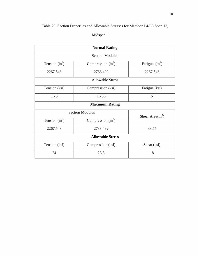
101

Table 29. Section Properties and Allowable Stresses for Member L4-L8 Span 13,

Midspan.

Normal Rating

Section Modulus

Tension (in3) Compression (in

3) Fatigue (in

3)

2267.543 2733.492 2267.543

Allowable Stress

Tension (ksi) Compression (ksi) Fatigue (ksi)

16.5 16.36 5

Maximum Rating

Section Modulus Shear Area(in

2)

Tension (in3) Compression (in

3)

2267.543 2733.492 33.75

Allowable Stress

Tension (ksi) Compression (ksi) Shear (ksi)

24 23.8 18

102

Rails

Wood-

Ties

Girders

Cross

Frames

Figure 67. Bridge C – Finite Element Model

Table 30. Comparison between FE Model and Simple Beam Analysis

Types of

Loading

Section

Span 13 Midspan, Normal Rating Span 13 Midspan, Maximum

Rating

FE Model Simple

Beam

Analysis

%

Difference FE Model

Simple

Beam

Analysis

%

Difference

286 Rail Car

Loading 169 66 156% 255 101 152%

103

APPENDIX C – quickBridge RESULTS

BRIDGE A

Truck definition

Number of axles

8

Axle No X W

1 0 71.5

X is the coordinate and

2 5.68 71.5

W the weight of the axle

3 25.27 71.5

Coordinate of axle 1 is 0

4 30.95 71.5 5 37.61 71.5 6 43.29 71.5 7 62.88 71.5 8 68.56 71.5

Bridge geometry

Number of span

1

Span No L q div

L is the length,

1 44.8 0 115

q uniform load and

div number of divisions

on a particular span

L and div must be > 0

104

Results

X Vmax Mmin Mmax

N Rmin Rmax

0.00 239.1 0.0 0.0

1 0.0 239.1

0.39 235.4 0.0 91.7

2 0.0 239.1

0.78 231.6 0.0 180.5 1.17 227.9 0.0 267.3 1.56 224.8 0.0 351.7 1.95 221.7 0.0 434.4 2.34 218.6 0.0 514.7 2.73 215.5 0.0 592.6 3.12 212.4 0.0 668.1 3.51 209.3 0.0 741.1 3.90 206.1 0.0 811.7 4.29 203.0 0.0 879.9 4.67 199.9 0.0 945.7 5.06 196.8 0.0 1009.1 5.45 193.7 0.0 1070.0 5.84 190.6 0.0 1128.5 6.23 187.5 0.0 1184.6 6.62 184.4 0.0 1238.2 7.01 181.5 0.0 1289.5

7.40 179.0 0.0 1340.2

7.79 176.6 0.0 1391.6 8.18 174.1 0.0 1441.0 8.57 171.6 0.0 1488.5 8.96 169.1 0.0 1534.0 9.35 166.6 0.0 1577.6 9.74 164.1 0.0 1619.2 10.13 161.6 0.0 1663.1 10.52 159.2 0.0 1709.5 10.91 156.7 0.0 1753.5 11.30 154.2 0.0 1795.0 11.69 151.7 0.0 1834.2 12.08 149.2 0.0 1870.9 12.47 146.7 0.0 1905.1 12.86 144.2 0.0 1940.4 13.25 141.7 0.0 1978.1 13.63 139.3 0.0 2014.0 14.02 136.8 0.0 2047.9 14.41 134.3 0.0 2079.9 14.80 131.8 0.0 2109.9 15.19 129.3 0.0 2138.0 15.58 126.8 0.0 2164.1 15.97 124.3 0.0 2188.4 16.36 121.8 0.0 2210.6 16.75 119.4 0.0 2231.0 17.14 116.9 0.0 2249.4

105

17.53 114.4 0.0 2266.4 17.92 111.9 0.0 2281.9 18.31 109.4 0.0 2295.5 18.70 106.9 0.0 2307.1 19.09 104.4 0.0 2316.8 19.48 101.6 0.0 2324.6 19.87 98.5 0.0 2330.4 20.26 95.4 0.0 2334.2 20.65 92.3 0.0 2336.2 21.04 89.2 0.0 2336.2 21.43 86.0 0.0 2334.2 21.82 82.9 0.0 2330.3 22.21 79.8 0.0 2324.5 22.59 79.9 0.0 2324.5 22.98 83.0 0.0 2330.3 23.37 86.1 0.0 2334.2 23.76 89.2 0.0 2336.1 24.15 92.3 0.0 2336.1 24.54 95.4 0.0 2334.2 24.93 98.5 0.0 2330.3 25.32 101.6 0.0 2324.5 25.71 104.5 0.0 2316.7 26.10 107.0 0.0 2307.0 26.49 109.4 0.0 2295.4 26.88 111.9 0.0 2281.8 27.27 114.4 0.0 2266.3 27.66 116.9 0.0 2249.5 28.05 119.4 0.0 2231.1 28.44 121.9 0.0 2210.7 28.83 124.4 0.0 2188.5 29.22 126.8 0.0 2164.2 29.61 129.3 0.0 2138.1 30.00 131.8 0.0 2110.0 30.39 134.3 0.0 2079.9 30.78 136.8 0.0 2048.0 31.17 139.3 0.0 2014.0 31.55 141.8 0.0 1978.2 31.94 144.3 0.0 1940.4 32.33 146.7 0.0 1905.2 32.72 149.2 0.0 1870.9 33.11 151.7 0.0 1834.2 33.50 154.2 0.0 1795.1 33.89 156.7 0.0 1753.5 34.28 159.2 0.0 1709.5 34.67 161.7 0.0 1663.1 35.06 164.2 0.0 1619.2 35.45 166.6 0.0 1577.5 35.84 169.1 0.0 1533.9 36.23 171.6 0.0 1488.4 36.62 174.1 0.0 1440.9

106

37.01 176.6 0.0 1391.5 37.40 179.1 0.0 1340.2 37.79 181.6 0.0 1289.4 38.18 184.4 0.0 1238.2 38.57 187.5 0.0 1184.5 38.96 190.6 0.0 1128.4 39.35 193.7 0.0 1069.9 39.74 196.8 0.0 1008.9 40.13 200.0 0.0 945.6 40.51 203.1 0.0 879.8 40.90 206.2 0.0 811.6 41.29 209.3 0.0 741.0 41.68 212.4 0.0 667.9 42.07 215.5 0.0 592.4 42.46 218.6 0.0 514.5 42.85 221.7 0.0 434.2 43.24 224.8 0.0 351.5 43.63 227.9 0.0 267.1 44.02 231.7 0.0 180.5 44.41 235.4 0.0 91.7 44.80 239.1 0.0 0.0

107

BRIDGE B

Truck definition

Number of axles

8

Axle No X W

1 0 71.5

X is the coordinate and

2 5.68 71.5

W the weight of the axle

3 25.27 71.5

Coordinate of axle 1 is 0

4 30.95 71.5 5 37.61 71.5 6 43.29 71.5 7 62.88 71.5 8 68.56 71.5

Bridge geometry

Number of span

1

Span No L q div

L is the length,

1 40 0 115

q uniform load and

div number of divisions

on a particular span

L and div must be > 0

108

Results

X Vmax Mmin Mmax

N Rmin Rmax

0.00 224.2 0.0 0.0

1 0.0 224.2

0.35 221.1 0.0 76.9

2 0.0 223.8

0.70 218.0 0.0 151.6 1.04 214.8 0.0 224.2 1.39 211.7 0.0 294.6 1.74 208.6 0.0 362.8 2.09 205.5 0.0 428.9 2.43 202.8 0.0 493.8 2.78 200.3 0.0 557.5 3.13 197.8 0.0 619.4 3.48 195.4 0.0 679.5 3.83 192.9 0.0 738.0 4.17 190.4 0.0 794.7 4.52 187.9 0.0 849.6 4.87 185.4 0.0 903.6 5.22 182.9 0.0 956.0 5.57 180.4 0.0 1006.6 5.91 178.0 0.0 1055.5 6.26 175.5 0.0 1102.7

6.61 173.0 0.0 1148.2

6.96 170.5 0.0 1191.9 7.30 168.0 0.0 1233.9 7.65 165.5 0.0 1274.2 8.00 163.0 0.0 1312.7 8.35 160.5 0.0 1349.6 8.70 158.1 0.0 1384.6 9.04 155.6 0.0 1418.0 9.39 153.1 0.0 1449.6 9.74 150.6 0.0 1479.5 10.09 148.1 0.0 1510.9 10.43 145.6 0.0 1550.3 10.78 143.1 0.0 1588.0 11.13 140.6 0.0 1623.9 11.48 138.2 0.0 1658.6 11.83 135.7 0.0 1692.0 12.17 133.2 0.0 1723.6 12.52 130.7 0.0 1753.5 12.87 128.2 0.0 1781.7 13.22 125.7 0.0 1808.1 13.57 123.2 0.0 1832.8 13.91 120.8 0.0 1855.8 14.26 118.3 0.0 1877.0 14.61 115.8 0.0 1896.5 14.96 113.3 0.0 1914.3 15.30 110.8 0.0 1930.3 15.65 108.3 0.0 1944.7 16.00 105.8 0.0 1957.2

109

16.35 103.3 0.0 1968.1 16.70 100.9 0.0 1977.2 17.04 98.4 0.0 1984.6 17.39 95.9 0.0 1990.3 17.74 93.4 0.0 1994.2 18.09 90.9 0.0 1996.5 18.43 88.4 0.0 1996.9 18.78 85.9 0.0 1995.7 19.13 83.4 0.0 1992.7 19.48 80.8 0.0 1988.0 19.83 77.7 0.0 1981.6 20.17 77.4 0.0 1981.6 20.52 80.5 0.0 1988.1 20.87 83.2 0.0 1992.9 21.22 85.7 0.0 1996.0 21.57 88.2 0.0 1997.4 21.91 90.6 0.0 1997.0 22.26 93.1 0.0 1994.9 22.61 95.6 0.0 1991.0 22.96 98.1 0.0 1985.4 23.30 100.6 0.0 1978.1 23.65 103.1 0.0 1969.1 24.00 105.6 0.0 1958.3 24.35 108.0 0.0 1945.8 24.70 110.5 0.0 1931.6 25.04 113.0 0.0 1915.7 25.39 115.5 0.0 1898.0 25.74 118.0 0.0 1878.6 26.09 120.5 0.0 1857.4 26.43 123.0 0.0 1834.5 26.78 125.5 0.0 1809.9 27.13 127.9 0.0 1783.6 27.48 130.4 0.0 1755.5 27.83 132.9 0.0 1725.7 28.17 135.4 0.0 1694.2 28.52 137.9 0.0 1661.0 28.87 140.4 0.0 1626.0 29.22 142.9 0.0 1589.3 29.57 145.4 0.0 1550.8 29.91 147.8 0.0 1510.9 30.26 150.3 0.0 1479.6 30.61 152.8 0.0 1449.8 30.96 155.3 0.0 1418.3 31.30 157.8 0.0 1385.0 31.65 160.3 0.0 1350.0 32.00 162.8 0.0 1313.3 32.35 165.2 0.0 1274.8 32.70 167.7 0.0 1234.7 33.04 170.2 0.0 1192.8 33.39 172.7 0.0 1149.1

110

33.74 175.2 0.0 1103.8 34.09 177.7 0.0 1056.7 34.43 180.2 0.0 1007.8 34.78 182.7 0.0 957.3 35.13 185.1 0.0 905.0 35.48 187.6 0.0 851.0 35.83 190.1 0.0 795.2 36.17 192.6 0.0 737.8 36.52 195.1 0.0 678.6 36.87 197.6 0.0 618.5 37.22 200.1 0.0 556.7 37.57 202.6 0.0 493.2 37.91 205.2 0.0 428.2 38.26 208.3 0.0 362.2 38.61 211.4 0.0 294.1 38.96 214.5 0.0 223.8 39.30 217.6 0.0 151.4 39.65 220.7 0.0 76.8 40.00 223.8 0.0 0.0

111

BRIDGE C

Truck definition

Number of axles

8

Axle No X W

1 0 71.5

X is the coordinate and

2 5.68 71.5

W the weight of the axle

3 25.27 71.5

Coordinate of axle 1 is 0

4 30.95 71.5 5 37.61 71.5 6 43.29 71.5 7 62.88 71.5 8 68.56 71.5

Bridge geometry

Number of span

1

Span No L q div

L is the length,

1 59.5 0 115

q uniform load and

div number of divisions

on a particular span

L and div must be > 0

112

Results

X Vmax Mmin Mmax

N Rmin Rmax

0.00 287.2 0.0 0.0

1 0.0 287.2

0.52 283.5 0.0 146.7

2 0.0 285.3

1.03 279.8 0.0 289.5 1.55 276.1 0.0 428.5 2.07 272.3 0.0 563.6 2.59 268.6 0.0 694.8 3.10 264.9 0.0 822.2 3.62 261.1 0.0 945.7 4.14 257.4 0.0 1065.4 4.66 253.7 0.0 1181.2 5.17 249.9 0.0 1293.2 5.69 246.2 0.0 1401.2 6.21 242.5 0.0 1505.5 6.73 238.7 0.0 1606.2 7.24 235.0 0.0 1704.6 7.76 231.3 0.0 1799.2 8.28 227.6 0.0 1889.9 8.80 223.8 0.0 1976.7 9.31 220.1 0.0 2059.7

9.83 216.4 0.0 2138.9

10.35 212.6 0.0 2230.2 10.87 208.9 0.0 2320.9 11.38 205.2 0.0 2407.8 11.90 201.4 0.0 2490.8 12.42 197.7 0.0 2569.9 12.93 194.0 0.0 2645.2 13.45 190.3 0.0 2716.6 13.97 186.5 0.0 2784.2 14.49 182.8 0.0 2847.8 15.00 179.1 0.0 2907.7 15.52 175.3 0.0 2963.7 16.04 171.6 0.0 3015.8 16.56 168.5 0.0 3064.0 17.07 165.4 0.0 3109.5 17.59 162.3 0.0 3152.0 18.11 159.2 0.0 3190.6 18.63 156.1 0.0 3225.3 19.14 152.9 0.0 3256.2 19.66 149.5 0.0 3283.2 20.18 145.8 0.0 3321.8 20.70 142.1 0.0 3364.3 21.21 138.4 0.0 3402.9 21.73 134.6 0.0 3437.6 22.25 131.5 0.0 3468.5 22.77 128.4 0.0 3495.5 23.28 125.3 0.0 3518.7 23.80 122.2 0.0 3538.0

113

24.32 119.1 0.0 3553.4 24.83 116.0 0.0 3565.0 25.35 112.6 0.0 3572.7 25.87 108.8 0.0 3576.6 26.39 105.1 0.0 3576.6 26.90 101.4 0.0 3572.7 27.42 97.7 0.0 3565.0 27.94 93.9 0.0 3553.4 28.46 90.2 0.0 3539.9 28.97 86.5 0.0 3536.7 29.49 82.7 0.0 3532.2 30.01 80.8 0.0 3529.5 30.53 84.6 0.0 3533.2 31.04 88.3 0.0 3542.3 31.56 92.0 0.0 3556.8 32.08 95.7 0.0 3567.5 32.60 99.5 0.0 3574.2 33.11 103.2 0.0 3577.2 33.63 106.9 0.0 3576.2 34.15 110.7 0.0 3571.4 34.67 114.4 0.0 3562.7 35.18 117.5 0.0 3550.2 35.70 120.6 0.0 3533.8 36.22 123.7 0.0 3513.6 36.73 126.8 0.0 3490.0 37.25 129.9 0.0 3463.9 37.77 133.1 0.0 3434.0 38.29 136.5 0.0 3400.3 38.80 140.2 0.0 3362.7 39.32 143.9 0.0 3321.2 39.84 147.6 0.0 3283.6 40.36 151.4 0.0 3257.5 40.87 154.5 0.0 3227.6 41.39 157.6 0.0 3193.9 41.91 160.7 0.0 3156.3 42.43 163.8 0.0 3114.8 42.94 166.9 0.0 3069.4 43.46 170.0 0.0 3020.3 43.98 173.4 0.0 2967.2 44.50 177.2 0.0 2910.3 45.01 180.9 0.0 2849.5 45.53 184.6 0.0 2784.9 46.05 188.3 0.0 2716.4 46.57 192.1 0.0 2644.0 47.08 195.8 0.0 2567.8 47.60 199.5 0.0 2487.7 48.12 203.3 0.0 2405.0 48.63 207.0 0.0 2319.1 49.15 210.7 0.0 2229.4 49.67 214.5 0.0 2139.0

114

50.19 218.2 0.0 2060.9 50.70 221.9 0.0 1978.9 51.22 225.7 0.0 1893.0 51.74 229.4 0.0 1803.3 52.26 233.1 0.0 1709.7 52.77 236.8 0.0 1612.2 53.29 240.6 0.0 1510.9 53.81 244.3 0.0 1405.8 54.33 248.0 0.0 1296.7 54.84 251.8 0.0 1183.8 55.36 255.5 0.0 1067.1 55.88 259.2 0.0 946.5 56.40 263.0 0.0 822.0 56.91 266.7 0.0 693.7 57.43 270.4 0.0 561.5 57.95 274.1 0.0 425.5 58.47 277.9 0.0 287.5 58.98 281.6 0.0 145.7 59.50 285.3 0.0 0.0

115

REFERENCES

1. Abhari, R. S., (2007), “Rehabilitation of Timber Railroad Bridges Using

Glass Fiber Reinforced Polymer Composite,” M.S. Thesis, West Virginia

University.

2. AREMA, (2000). “AREMA Manual of Engineering,” Chapter 8 and

Chapter 15, American Railway Engineering and Maintenance-of-Way

Association,

3. Calcada, R., Cunha, A., and Delgado, R. (2002), “Dynamic Analysis of

Metallic Arch Railway Bridge,” Journal of Bridge Engineering, Vol.7,

No.4, pp.214-222.

4. Chajes, M.J., Shenton III, H.W., Finch Jr, W.W. (2001), “Diagnostic and

In-Service Testing of Transit Railway Bridge,” Transportation Research

Recor, No.1770, pp.51-57.

5. DelGrego, M.R., Culmo, M.P., and DeWolf, J.T. (2008), “Performance

Evaluation through Field Testing of Century-Old Railroad Truss Bridge,”

Journal of Bridge Engineering, Vol.13, No.2, pp.132-138.

6. Gutkowski, R.M., Shigidi, A.M., Tran, A.V., Peterson, M.L. (2001),

“Field Studies of Strengthened Timber Railroad Bridge,” Transportation

Research Record, No.1770, pp.139-148.

7. Gutkowski, R.M., Shigidi, A.M., Tran, A.V., Peterson, M.L. (2003),

“Field Investigation of a Strengthened Timber Trestle Railroad Bridge,”

Department of Civil Engineering, Colorado State University.

8. Kober, A. C., et al., (2003) “Rehabilitation of the Historic Kate Shelley

High Bridge,” AREMA 2003 Proceedings.

9. Leighty III, C.A., Laman, J.A., and Gittings, G.L. (2004), “Heavy Axle

Study: Impact of Higher Rail Car Weight Limits on Short-Line Railroad

Bridge Structures,” Civil Engineering and Environmental Systesms,

Vol.21, No.2, pp.91-104.

10. Majka, M. and Hartnett, M. (2009), “Dynamic Response of Bridges to

Moving Trains: A Study on Effects of Random Track Irregularities and

Bridge Skewness,” Computers and Structures, Vol.87, pp.1233-1252.

116

11. Malm, R. and Andersson, A., (2006), “Field Testing and Simulation of

Dynamic Properties of a Tiled Arch Railway Bridge,” Engineering

Structures, Vol.28, pp.143-152.

12. Radford, D.W., VanGoethem, D., Gutkowski, R.M., Peterson, M.L.

(2002), “Composite Repair of Timber Structures,” Construction and

Building Materails, Vol.16, pp.417-425.

13. Song, M, Noh, H, Choi, C. (2003), “A New Three-Dimensional Finite

Element Analysis Model of High-Speed Train-Bridge Interactions,”

Engineering Structures, Vol.25, No.13, pp.1611-1626.

14. Taljsten, B. and Carolin, A., (1998) “Strengthening of a Concrete Railway

Bridge in Lulea with Carbon Fibre Reinforced Polymers-CFRP,” Project

Report, Lulea University of Technology, Sweden.

15. WestBrook Associated Engineers, E8 plus Constructors (2006), “Impact

of Railcar Weight Chanes on Bridges of the State of Wisconsin-owned

Railroad Systems,” Wisconsin DOT Research, Development &

Technology Transfer, Final Report No. 0092-05-13, Wisconsin DOT.

16. Horney, J. (2003, October 5-8). “Capability Evaluation of Short Line

Timber Trestles to handle 286K Loads, ” American Short Line and

Regional Railroad Association/Federal Railroad Administration, AREMA

Conference Presentation, Carter & Burgess, Chicago, IL.

17. Uppal, A.S (2005, September). “Coping with the older Railroad Steel

Bridges,” IMA Infrastructure Engineering Inc. Edmonton, Alberta,

Canada.

18. Turkkan, N.” quickBridge Moment and Shear Envelopes V1.2 – 2001”,

Universtite de Monton, Moncton, N.B. Canada.

19. Unsworth, J.F. “Evaluation of the Load Capacity of a Rehabilitated Steel

Arch Railway Bridge,” Canadian PacificRailway, Calgary, Alberta,

Canada.

20. Chebrolu, K, Raman, B, Mishra N, Valiveti, P.K, Kumar,R. “ BriMon: A

sensor Network System for Railway Bridge Monitoring,’ Indian Institue of

Technology, Kanpur (2008).

21. Commander, B, Varela-Ortix, W, Stanton T.R, (May 2009) “Field Testing

and Load Rating Report. Brdige FSBR-514, Fort Shafter, Hawaii”, US

117

Army Corps of Engineers.

22. Harris, F.R. (1994, May), “Bridge Evaluation Survey Report of Bridge A,

1st Cycle”.

23. Polytran Engineering Associates, PC, (2001, February) “Inspection Report

for Bridge A, Cycle 2.”

24. Polytran Engineering Associates, PC, (2005, December) “Inspection

Report for Bridge A, Cycle 3.”

25. Harris, F.R. (1989, August), “Bridge Evaluation Survey Report of Bridge

D, 1st Cycle”.

26. Baker, M. Jr., Inc. (1996, April) “Inspection Report for Bridge D, Cycle

2.”

27. Nassif, H.H., Suksawang, N., Davis, J.C. (2007, January). “Evaluation of

Bridge Deck Cracking on the Delaware River Turnpike Bridge.”

28. Nassif, H.H., Kwon, G, Su, D. (2008, January). “Behavior of Early Age

Concrete Deck on the Hackensack River Bridge.”

29. ABAQUS User Manual.

30. Parsons Transportation Group, (May 20, 2002), “Inspection Cycle

Number 3, Bridge C.”

31. Chas. H. Sells, Inc. (August 23, 2007), “Inspection Cycle Number 4,

Bridge B.”