Rural Public Transportation: Using Geographic Information Systems … · · 2018-02-22Rural Public Transportation: Using Geographic Information Systems to Guide Service ... Gravity

Final Technical Report TNW2002-01

Research Project Agreement No. 922910, Task 2

Rural Public Transportation: Using Geographic Information Systems to Guide Service Planning

Rural Public Transportation: Using Geographic Information Systems

to Guide Service Planning

by

Thomas W. Sanchez Center for Urban Studies, Transportation Research Group

Portland State University, Portland, OR

Neil Bania Laura Leete

Public Policy Research Center Willamette University, Salem, OR

Report prepared for: Transportation Northwest Regional Center (TransNow)

Department of Civil Engineering 129 More Hall

University of Washington, Box 352700 Seattle, WA 98195-2700

(REVISED) June 2002

DISCLAIMER

The contents of this report reflect the views of the authors, who are responsible for the facts and

the accuracy of the data presented herein. This document is disseminated through Transportation

Northwest (TransNow) Regional Center under the sponsorship of the Department of

Transportation UTC Grant Program in the interest of information exchange. The U.S.

Government assumes no liability for the contents or use thereof. The contents do not necessarily

reflect the views or policies of the U.S. Department of Transportation or any of the local

sponsors.

i


TABLE OF CONTENTS

I. INTRODUCTION ..................................................................................................................1

Rural Living in the U.S...........................................................................................................2 Welfare Reform Increases the Need for Public Transportation..............................................3 Rural Transportation Challenges ............................................................................................4 Can Technology Help? ...........................................................................................................5 GIS Technology......................................................................................................................6

II. COMMUNITY EXAMPLES ...............................................................................................10 The Central Massachusetts Regional Planning Commission ...............................................10 San Luis Obispo Council of Governments, San Luis Obispo County, California................15 St. Mary’s County, Maryland ...............................................................................................19

III. SUMMARY OF THE CASES..............................................................................................22 Limitations to the GIS Analysis Used in the Community Cases ..........................................23

IV. OREGON CASE STUDIES .................................................................................................25 Central Oregon......................................................................................................................26

Institutional Home for Transit Planning........................................................................29 Data and Analysis ..........................................................................................................31

Florence, Oregon...................................................................................................................35 Institutional Home for Transit Planning........................................................................38 Data and Analysis ..........................................................................................................40

Discussion.............................................................................................................................42 V. ROLE OF GIS.......................................................................................................................44

Role of GIS in Transportation Modeling Efforts..................................................................45 GIS and Economic Activity ..................................................................................................46 GIS Tools - Accessibility, Gravity Models, and Spatial Interaction ....................................48

VI. RURAL PUBLIC TRANSPORTATION ACCESSIBILITY MODEL ...............................49 Steps in the Model ................................................................................................................50

Step One. Define service area boundaries....................................................................50 Step Two. Map appropriate origins and destinations of targeted population. .............51 Step Three. Overlay grid system to aggregate transportation supply and demand information.....................................................................................................................53 Step Four. Analysis of transit supply and demand characteristics...............................58 Step Five. Performance evaluation. ..............................................................................62

City of Florence, Rhody Express Example...........................................................................63 Tillamook County Transportation District Example ............................................................66 Bend-Redmond Shuttle Example..........................................................................................67 Model Limitations.................................................................................................................69

VII. SUMMARY AND CONCLUSIONS ...................................................................................69 VIII. REFERENCES .....................................................................................................................72 IX. APPENDICES ......................................................................................................................77

Appendix A...........................................................................................................................77 Appendix B ...........................................................................................................................79

ii

List of Tables

Table 1: Data types and sources.....................................................................................................32 Table 2: Data types and sources.....................................................................................................41 Table 3: Mapping data and sources ...............................................................................................53 Table 4: Example trip purpose weights derived from 1995 NPTS data ........................................59

List of Figures Figure 1: Central Massachusetts Regional Planning Area.............................................................11 Figure 2: San Luis Obispo Council of Governments Planning Area.............................................16 Figure 3: Case study locations .......................................................................................................25 Figure 4: Central Oregon Region...................................................................................................27 Figure 5: Florence, Oregon ............................................................................................................36 Figure 6: Example origin and destination map ..............................................................................55 Figure 7: Gridded employment map ..............................................................................................56 Figure 8: Gridded TANF recipient locations .................................................................................57 Figure 9: Gravity model output for existing conditions.................................................................61 Figure 10: Gravity model output for proposed transit system .......................................................61 Figure 11: Gridded TANF recipient and employment location map.............................................64 Figure 12: Transit service route maps............................................................................................65 Figure 13: Tillamook County Transportation District ...................................................................67 Figure 14: Proposed Bend-Redmond Shuttle ................................................................................68 ACKNOWLEDGEMENTS The researchers would like to acknowledge the support of the Oregon Department of Transportation (ODOT) for this research project. The research also benefited from the assistance of Alan Kirk (ODOT), Barnie Jones (ODOT), Robin Phillips (ODOT), Nick Fortey (FHWA), and Terry Parker (Lane Transit District).

1


I. INTRODUCTION

Rural communities throughout the U.S. have a unique set of characteristics; these same rural

communities have an equally unique set of service needs. A common trait belonging to many

rural communities is the difficulty that governmental agencies have in providing sufficient public

transportation for them. The goal of this project was to explore the nature of rural living, with a

focus on transportation issues as they relate to social service provision. The project investigated

existing methodologies used to analyze transit service, and developed a model using Geographic

Information Systems (GIS) to obtain quantifiable measurements that could be used to evaluate

transportation accessibility improvements in rural areas. With a GIS model, rural transportation

planners and social service providers might be better equipped to coordinate, evaluate, improve

and monitor transit services in rural communities.

In the remainder of this introductory chapter, we provide an overview of public

transportation provision in rural areas of the U.S., the relationship between public transportation

needs, welfare-to-work reform efforts, and the challenges that derive from an ever-evolving rural

economy. This is followed by a brief overview of GIS technologies, its conceptual

underpinnings and the application of GIS to transportation and social service planning. In the

subsequent chapters of this report we give a detailed explanation of a GIS model that can be used

to quantify spatial relationships in transportation planning as it relates to welfare-to-work

services and goals. We then provide two case studies of transit/welfare-to-work planning efforts

within Oregon – in Lane County and Bend – and discuss the application of a proposed GIS

model. In the final chapter, we draw general conclusions regarding the utility of the model

developed here, barriers to its full application and possible future extensions.

2

Rural Living in the U.S.

Public transportation service in rural U.S. communities has historically been less

adequate than that provided by urban public transit systems. Most of the disparity between urban

and rural public transportation is due strictly to the nature of what it means to be rural. Rural

areas are by definition remote, sparsely populated, and often dependent on geographically

dispersed natural resource based industries and agriculture for their economic base. The distance

from sizeable population clusters and large centralized markets makes rural areas less attractive

to potential residents, businesses and industries that are not natural resource or agriculture

oriented (Kilkenney 1998). The long distances between rural residences, employment

opportunities and necessary services create significant unmet need for transportation options in

rural communities. At the same time, providing public transportation in remote areas is

especially complex and expensive (Kihl, Knox and Sanchez 1997).

Rural communities are commonly served by county governments, whose umbrella of

responsibility often covers vast areas but are often limited by small tax bases. The greater

distances to cover, coupled with small populations, makes traditional (fixed route, fixed

schedule) public transportation economically infeasible in most rural areas (Casavant and

Painter 1998). A study by the National Personal Transportation Survey (NPTS) suggests that

close to eighty percent of all non-metropolitan counties have no public bus service and ninety

percent of all non-metropolitan area commutes are made in private vehicles (Fletcher and Jensen

2000).

A prominent yet frequently overlooked characteristic of rural communities is the level of

poverty that affects many rural residents. Poverty in U.S. central cities has received significant

attention and has greatly influenced the perception of “who is poor.” It is not often recognized,

3

however, that rural areas have higher rates of poverty than metropolitan areas. For example, in

1990 approximately sixteen percent of the rural population was living in poverty, while about

twelve percent of the metropolitan population was. It has also been found that the rural poor

have a greater tendency to be chronically poor than do their urban counterparts (Findeis and

Jensen 1998). The level of poverty that is experienced by the rural population intensifies the

need for transportation services, as many rural people cannot afford to buy or maintain private

vehicles.

Welfare Reform Increases the Need for Public Transportation

Many of the more unfortunate characteristics of rural living have been exacerbated by the

passage of the 1996 Personal Responsibility and Work Opportunity Reconciliation Act

(PRWORA). With the objective of moving people off welfare and permanently into the work

force, the passage of PRWORA has deepened the needs of rural residents for reliable

transportation. According to the U.S. Department of Health and Human Services, only about six

percent of welfare recipients own an automobile (U.S. GAO 1998). While most welfare

recipients live in either central cities or rural areas, employment opportunities have been steadily

migrating to the suburbs over the past several decades. A recent study found that about forty-one

percent of jobs are now located in the suburbs (Nightingale 1997). The trend to a strong

suburban employment base along with the loss of traditional rural employers has caused an

increase in the distance between the rural poor and permanent jobs. Agriculture, resource

extraction and manufacturing (mostly dealing with the processing of agricultural and natural

resources), along with associated services, were the traditional underpinning of rural economies.

In recent years, however, these rural industries have lost ground out to foreign competition,

4

especially in the area of resource extraction (Fawson, et al. 1998). There has also been

considerable movement of light manufacturing industries from rural to suburban locations.

Historically, the bulk of rural manufacturing jobs utilized low-skilled labor to produce

relatively simple products (Freshwater 1996). These jobs, along with associated service sector

jobs, constituted the type of employment opportunities generally needed for people transitioning

from welfare to work. Thus, just at the time that rural areas have suffered from a significant loss

of important employment opportunities, the passage of PRWORA has increased the number of

job seekers, creating a profusion of unemployment. Since the inception of PRWORA, social

service agencies and local governments have been grappling to find solutions to employment

disparities in rural communities, as well as find ways to provide transportation services to

suburban jobs.

Rural Transportation Challenges

Facilitating appropriate transportation services for the rural poor transitioning from

welfare into regular employment can be an intricate act, balancing many individual needs with

factors unique to rural living. The three most outstanding elements that must be contended with

when providing transportation for the rural poor are the hours of service needs, existing route

limitations and distance to employment opportunities (Nightingale 1997). Almost twenty-four

percent of non-metropolitan residents over eighteen years of age do not have a high school

diploma (RUPRI 1998). This lack of education seriously affects the types of employment open

to many, limiting them to service sector or unskilled manufacturing jobs. Such jobs frequently

call for non-traditional work hours, such as night, swing and weekend shifts. And non-standard

work hours complicate the ability of social service and local transit agencies to provide

5

transportation for the rural poor, as existing public transportation is typically not available at

non-standard times (Kaplan 1997).

Traditional public transportation routes are generally focused on either local (within

municipality) or on commuter services that usually follow a direct “express” route from the

suburbs into the central city. Since the rural poor live outside the general pattern of existing

transit routes and the majority of service sector and light manufacturing jobs have moved to the

suburbs, a need for “reverse commute” services has emerged (Ward 2000). Reverse commute

entails providing public transportation from both the central city and from the outlying (rural)

areas into the suburbs, essentially reversing the traditional public transportation patterns.

Distance serves as the principal accessibility barrier to employment among the rural poor,

who frequently lack access to both dependable automobiles and adequate public transit (Fletcher

and Jensen 2000). The same factors have also proven to be significant in leading many of the

rural poor to accept low-wage and/or part-time jobs that are close to home (Pindus 2001).

Transportation availability is an especially salient factor for the single parent households who

accounted for about seventy-five percent of total AFDC recipients in 1995. The employment

choices of a single parent are severely limited by childcare locations and schools, making

transportation availability paramount to their success in transitioning from welfare to work

(Accordino 1998).

Can Technology Help?

For rural agencies, faced with scarce fiscal resources, low levels of demand and

understaffed facilities, serving the rural poor with viable transportation options can seem an

almost insurmountable task (Marks, et al. 1999). Access to appropriate technological solutions

can be the determining factor in the ability to meet transportation challenges. Investment in

6

computer technology that can be used in social service and transportation applications has

become relatively common in large urban agencies. Rural agencies are also, albeit slowly,

beginning to see the benefits of applying computer technologies within their jurisdictions

(Zarean, et al. 1998). GIS is an important technology that is increasingly being used to support

transportation planning. The mapping capabilities of a GIS can provide decision makers with a

powerful tool to analyze mobility and accessibility issues within their jurisdictions in both visual

and quantifiable terms (CTAA 2000).

GIS Technology

According to Environmental Systems Research Institute Inc. (ESRI), “Desktop GIS

represents the real world on a computer similar to the way maps represent the real world on

paper” (ESRI 1997). A GIS with its roots intertwined in geography, cartography and computer

science is (at a very basic level) computer software that is designed to answer questions that

relate to locations, patterns, trends, and conditions. A GIS can answer questions directly related

to planning applications such as:

• Where are particular features found?

• What geographic patterns can be found?

• Where have changes occurred over a given time period?

• Where do certain conditions apply?

• What are the spatial implications if an organization takes a certain action? (Heywood, et

al. 1998).

7

A GIS is akin to a computerized map that is linked to a database. The objects represented on a

GIS map are referred to as geographic features, with each feature having a description included

within the database.

Many advantages of using GIS for transportation modeling have been identified by

researchers. The primary advantages include speed, analytical capabilities, visual power,

efficiency of data storage, integration of spatial databases, and capabilities for “finer-grained”

spatial analysis (Hartgen, Li and Alexiou 1993; Anderson 1991; Niemeier and Beard 1993). By

its nature, geographic information is rarely beneficial to only a single user or location. Typically

geographic attributes are common to region-wide locations. Initial start-up investments in GIS

usually involve large investments in base map layers of geographical data. For example, cities

will often want countywide data because planning activities usually account for extra-

jurisdictional areas to accommodate growth. Environmental data is typically collected and

maintained by a state or regional organization, transportation facility data is handled by state,

county, and/or local agencies, business data may be available locally, etc. It is not unusual for

these different types of data to be collected and reassembled by individual users. This may be a

function of different data needs related to accuracy, software compatibility, and geographic

resolution among organizations. A GIS can serve to integrate all of these data types from

different data sources (Simkowitz 1990).

It is not unusual for users to be unaware of available data that meet their operational

requirements. Better communications, coordinated data collection efforts, and information

exchange can in the long run lead to cost savings and better decision-making (Onsrud and

Rushton 1995). Dueker and Vrana (1995) generally refer to these as efficiency, effectiveness,

and enterprise benefits. Agency efficiency and effectiveness benefits are most commonly

discussed in the literature. The third type of benefits, enterprise benefits, take the form of overall

8

information management activities within an organization. An example of interagency

cooperation that can produce enterprise benefits is the case of the Pennsylvania Department of

Transportation (PennDOT). The process that PennDOT used in constructing their GIS system

included the input and from the state departments of agriculture, commerce, community offices,

environmental resources, state data center, state library, and governor’s office (Basile, TenEyck

and Pietropola 1991). Such a comprehensive approach in the initial phases of database

construction anticipates future data integration and sharing opportunities, as well as providing

the collective experience to establish a durable GIS system. By having access to an increased

amount of information, individual organizations can enhance their own data resources. Spatial

data when combined or overlaid can result in a synergistic effect - the combination of layers is

more valuable than the sum of the individual layers (Evans and Ferreira 1995). This type of

data enrichment is another benefit that can be realized by organizations that share data.

The capabilities of a GIS in planning applications are enormous and can be tailored to

very explicit uses. More specifically, for coordinating social services and rural transportation

planning a GIS can be used to:

• Illustrate the spatial mismatch between welfare-to-work participants and potential

employment opportunities.

• Assist in determining a person’s access to appropriate transit services.

• Estimate the prospective number of transit users in a defined area.

• Suggest methods to implement new transit services or modify existing routes by

identifying clusters of possible riders and likely destinations (Multisystems 2000).

As GIS technology has become more “user friendly” and less expensive it has also

become relatively common in transportation and social service planning applications. The U.S.

9

Department of Transportation (U.S. DOT) has created a list of essential data layers and

information on where to find the data when using a GIS in welfare-to-work programs U.S.

DOT’s list includes:

• Welfare Population – where the welfare population live, location of recipient residences.

Data sources: State or county human service agencies.

• Employment – location and availability of job opportunities for which the Temporary

Assistance for Needy Families (TANF) recipients may be qualified.

Data sources: State labor and workforce development agencies, private industry councils,

and metropolitan planning organizations.

• Training Centers – location of training centers that TANF recipients may attend to

receive job-training skills.

Data Sources: State or county human service agencies.

• Childcare Facilities – location of childcare facilities that TANF recipients may patronize.

Data Sources: State and county child care service agencies.

• Transportation – location and schedule of public transportation routes and the

availability and extent of existing social service transportation, paratransit, carpooling,

and vanpooling service areas.

Data Sources: local transit providers, metropolitan planning organizations, FTA

National Transit GIS databases

• Hours of Operation – frequency of transportation services and business hours for

employment, child and day care facilities.

Data Sources: Local transportation providers (U.S. DOT 1998)

10

Many of the agencies that have taken advantage of GIS technology to help address

transportation issues within welfare to work applications, have used U.S. DOT’s suggested

formula. By overlaying the recommended layers, various agencies have been able to generate

visual representations of their transportation systems in relation to welfare recipients and

potential places of employment. Most commonly, jurisdictions have utilized geographic

buffering analysis techniques. A buffering application allows the user to determine factors such

as the number of job seekers living within a chosen distance from existing transit routes or stops.

The buffers can be set for quarter and half-mile distances to analyze how many people are

actually within walking distance to public transportation (SLOCOG 1998). These are common

measurements used for acceptable walking distances to transit. (See Lam and Morrall 1982 and

Schoppert and Herald 1978 for a discussion of walking access to transit.) Examples of how GIS

technology has been used to narrow the gap between welfare-to-work persons and job

opportunities by improving transportation services are nicely demonstrated in the cases of the

Central Massachusetts Regional Planning Commission (CMRPC 2000), the San Luis Obispo

Council of Governments (SLOCOG) and St. Mary’s County Department of Social Services.

II. COMMUNITY EXAMPLES

The Central Massachusetts Regional Planning Commission

The Central Massachusetts Regional Planning Commission (CMRPC) is a regional

planning agency whose jurisdiction encompasses central and southern Worchester County and

portions of southern Middlesex County. Most of CMRPC area’s population is concentrated in

the City of Worcester; therefore, much of its demographic data reflects urban characteristics.

There are a total of fifty-nine communities included in CMRPC’s planning area, however, and

many fit the classic description of rural areas (Figure 1).

11

Figure 1: Central Massachusetts Regional Planning Area

County data does not exactly match the CMRPC’s boundaries, but it does give a good

illustration of the area’s overall population trends. Data for Middlesex County indicates that it is

the more urban of the two counties, with approximately ninety-two percent of its total population

in urban areas and eight percent in rural areas (farm population is not included). Worchester

12

County is seventy-two percent urban and twenty-seven percent rural (U.S. Census 1990).

Another measure of the urban/rural nature of the two counties is population density. Middlesex

County has about 1,781 persons per-square mile; Worchester has 496 persons per-square mile

(U.S. Census 2000). Clearly Worchester can be characterized as more rural than Middlesex.

Both counties’ ethnic compositions are predominantly white. Middlesex is close to eighty-four

percent non-Hispanic white, six percent Asian, five percent Hispanic and three percent black;

Worchester is about eighty-six percent non-Hispanic white, seven percent Hispanic, and three

percent each Asian and black. The median annual income for Middlesex County is $53,268,

well above the Massachusetts state average of $43,015. The average income Worchester County

is slightly below the state average at $40,489.

Persons living below poverty account for about seven percent of the population of

Middlesex County and eleven percent live in Worchester County. About twenty-four percent of

Middlesex’s population are under eighteen and thirteen percent are over sixty-five years of age;

the demographics in Worchester County are somewhat similar. The CMRPC assumed the

responsibility of welfare-to-work (WtW) transportation planning from the Worchester Regional

Transit Authority (WRTA) in 1997. The two agencies have developed a good working

relationship, along with the Southern Worchester County Regional Employment Board and the

three additional Departments of Transitional Assistance in the region. Within the CMRPC’s

project area, only fourteen out of fifty-nine communities possess a fixed route transit service and

only one community has extensive service. CMRPC’s Sandi Johnson described the

transportation situation as follows, “The majority of our region is rural in nature, and very hard

to deal with” (Johnson 2001).

GIS technology is being used for the CMRPC’s transportation project’s analysis and

visual components. Most of the CMRPC’s project is conducted with the use of ESRI’s Arc-

13

`View and Arc/Info software, but also includes the use of IDRISI, TransCAD and Mapitude

programs. A typical CMRPC analysis involves overlaying the data recommended by U.S. DOT,

which includes the residential locations of welfare recipients, (zip+4, a postal designation that

identifies a structure or building and is not associated with an individual, was used to protect

recipient confidentiality) childcare provider locations, education and job-training facilities and

public transit routes. In addition to the basic layers, CMRPC added the locations of public

housing as well as the locations of manufacturing, industrial and service sector employers. The

additional layers were included to better match the job-seeking population with those businesses

most likely to hire entry-level workers.

The vision held by CMRPC was to develop an Internet based GIS “Trip Planner” that

could be used as a job placement tool. A trip planner uses geographic information (locations of

specific destinations such as jobs sites, social service offices and bus stops) and creates a trip

itinerary that can help determine the most efficient routes to take to a desired location. The trip

planner was foreseen by CMRPC as way to help WtW job placement services, human resource

personal, job training providers and employers route their clients and employees to work,

training programs and childcare destinations. The CMRPC’s GIS mapping capabilities have also

been used for a region-wide transportation mobility analysis. Trip Planner is still being

developed by CMRPC, while they are already enjoying the benefits of their GIS mapping

program.

One of the primary advantages CMRPC has garnered from using GIS technology in

transportation and WtW analysis is the easy identification of spatial mismatches between WtW

clients, transit and employment opportunities. This is usually done by identifying geographically

dispersed or separated residential locations and employment locations that are also ill-served by

transit services. Staff members are able to determine the proximity of welfare recipients to

14

existing bus routes and identify areas where gaps in transit service exist. Recognizing the fact

that many entry-level jobs require non-traditional work hours, CMRPC staff has also added

attribute data to employer descriptions that identifies those who require night, weekend and

swing shifts. The irregular work hour data has been used to determine the most effective

changes to be made to transit route service times, especially with regard to late night service.

Through a series of interviews with local employers, CMRPC found that by extending merely

nine of WRTA’s twenty-nine bus routes, an additional twenty-nine employers, seven hospitals

and hundreds of employees could be served by transit.

CMRPC was caught by surprise when GIS was used to illustrate demographic data. With

the GIS mapping application it discovered that sixty-four percent of the total welfare recipient

population lived in the city of Worchester, and among those, ninety-five percent lived within a

quarter mile of a bus route. The CMRPC staff also found that ninety-nine percent of childcare

providers and ninety-five percent of manufacturing and service sector employers were located

within a quarter mile of existing bus routes. An analysis of these findings concluded that even

though social services staff had previously known about the local transit system, they were not

aware of its coverage or how pivotal it could be in helping WtW persons find and maintain

employment. In light of this, a new “train the trainer” educational program has been designed to

teach job placement staff how to use the bus system. An educated staff can subsequently inform

their clients of transit options that could very well be crucial to WtW clients finding and

maintaining employment.

As with any project, CMRPC’s transit WtW project has had its limitations. Obtaining

and maintaining accurate up-to-date residential information on welfare recipients and on

employment opportunities was, and continues to be, the most challenging factor for the CMRPC

project. Confidentiality issues also had to be contended with when using residents’ address data.

15

Completion of the trip planner is far behind CMRPC’s projected schedule. The scope of

CMRPC’s project requires a high level of expertise from many fields. Very few public agencies

have the funding for this level of staffing and many of CMRPC’s staff had to learn complicated

technologies as they were being implemented. Furthermore, GIS software, along with other

software used to support the project, was expensive and funding has been an issue.

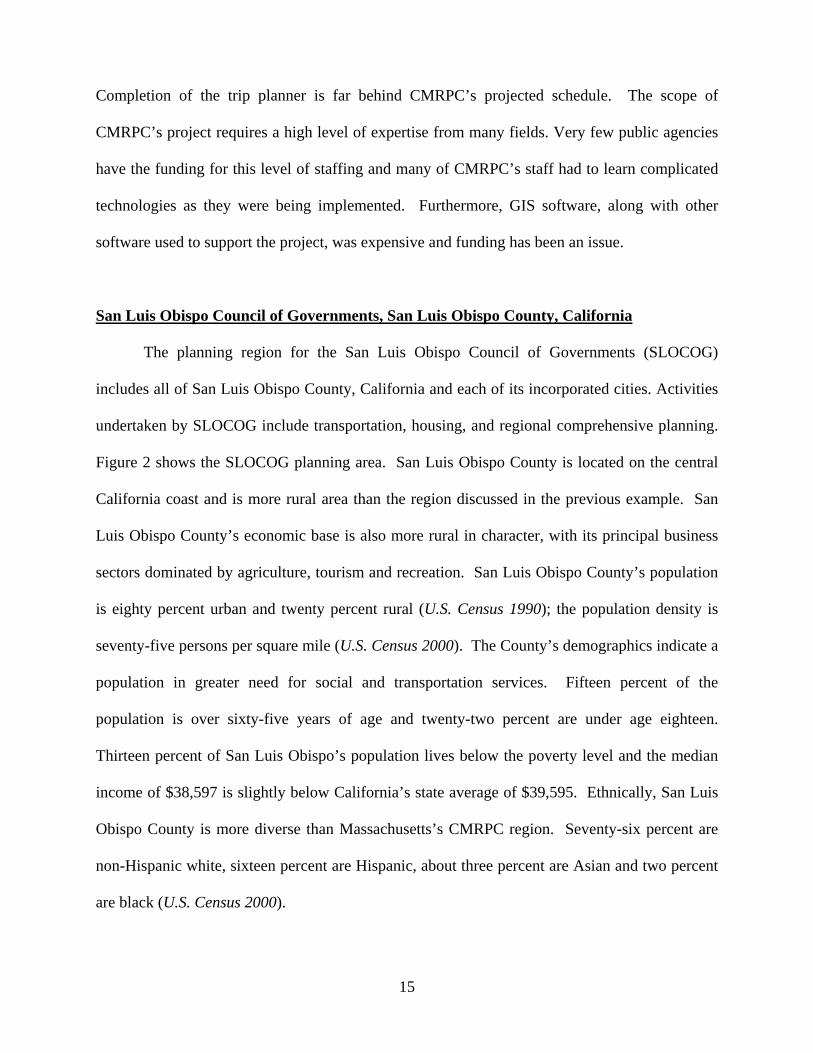
San Luis Obispo Council of Governments, San Luis Obispo County, California

The planning region for the San Luis Obispo Council of Governments (SLOCOG)

includes all of San Luis Obispo County, California and each of its incorporated cities. Activities

undertaken by SLOCOG include transportation, housing, and regional comprehensive planning.

Figure 2 shows the SLOCOG planning area. San Luis Obispo County is located on the central

California coast and is more rural area than the region discussed in the previous example. San

Luis Obispo County’s economic base is also more rural in character, with its principal business

sectors dominated by agriculture, tourism and recreation. San Luis Obispo County’s population

is eighty percent urban and twenty percent rural (U.S. Census 1990); the population density is

seventy-five persons per square mile (U.S. Census 2000). The County’s demographics indicate a

population in greater need for social and transportation services. Fifteen percent of the

population is over sixty-five years of age and twenty-two percent are under age eighteen.

Thirteen percent of San Luis Obispo’s population lives below the poverty level and the median

income of $38,597 is slightly below California’s state average of $39,595. Ethnically, San Luis

Obispo County is more diverse than Massachusetts’s CMRPC region. Seventy-six percent are

non-Hispanic white, sixteen percent are Hispanic, about three percent are Asian and two percent

are black (U.S. Census 2000).

16

Figure 2: San Luis Obispo Council of Governments Planning Area

In reaction to CalWORKS (California’s welfare to work program), SLOCOG initiated a

comprehensive transportation mobility study in 1997. The study was undertaken through a

cooperative effort by SLOCOG, the Private Industry Council, transit providers, social service

agencies, childcare providers and employers throughout San Luis Obispo County. The study

was designed to identify and eliminate transportation barriers keeping welfare recipients from

finding employment. Key to the analysis was examining transportation demand (origins and

destinations of CalWORKS recipients) in conjunction with existing transportation options

(supply). Supply and demand analysis was used in order to identify gaps in transportation

resources created by geography, time of day or day of the week. This was done by using a GIS

17

(ESRI’s ArcView) to map known origins and destinations and then visually interpreting the

results.

The SLOCOG staff used data that included the following:

• a list of childcare providers in the area and the number of permitted childcare slots;1

• employment sites (employment data was acquired from the Employment

Development Department);

• career training centers;

• CalWORKS recipient’s addresses (this data, like childcare, is considered

confidential); and

• all of the existing transportation resources (included all local and regional bus

services as well as a runabout service, rideshare program, ride-on program,

Greyhound bus service and Amtrak train service).

The data was entered into the GIS system and then each data layer was systematically

compared to the transit route data through GIS mapping. Creating quarter-mile buffers around

each existing transit route also allowed a transportation accessibility analysis to be performed.

Any area where CalWORKS recipients lived that was located outside of the buffers was

considered an area that needed transit route modification.

Visual analysis provided by the GIS created an abundance of information concerning the

status of transportation in San Luis Obispo County. The GIS allowed the development of

potential travel patterns through mapping known origins and destinations (such as residential and

1 These data were obtained from the California State Licensing Department, but information on available childcare openings was not released due to confidentiality concerns.

18

employment locations), which was very helpful in the SLOCOG study, as they had no empirical

data on the actual travel patterns of the CalWORKS recipients. One significant finding was that

seventy-five percent of the CalWORKS participants already lived within a quarter mile of a

transit line, and fifty-eight percent were within a quarter mile of a bus stop. With the majority of

participants living within walking distance of a transit route, SLOCOG realized that their efforts

and resources would be best spent on extending service times throughout the day, as large gaps

in service were found during non-traditional work hours.

At the time of the study, the regional transit service only operated between 6:00 a.m. and

6:30 p.m., and the most extensive local route only ran from 6:30 a.m. to 7:30 p.m. Specific

routes were targeted for increased service frequency, particularly mid-day and nighttime services

to area employment centers. This service changes were a response to feedback received from

riders and employers in the area.

Most of the region’s transportation service was found to be geographically adequate for

CalWORKS participants. The one exception was a rather remote community (Nipomo) that had

both a relatively high number of welfare recipients and virtually no transit service. Nipomo

ended up as a principal focus community for future transit improvement efforts. The GIS

analysis also yielded a number of other important observations. First, they found that a few

minor route modifications would greatly improve service to several area cities that provide much

of the employment opportunities.

Second, most of the area’s childcare providers were located along existing transit routes.

Sixty-three percent of the childcare facilities were found to be within one-quarter mile of transit

services and seventy-one percent of CalWORKS recipients lived within a quarter mile of

childcare services. In an interesting parallel to the analysis done by CRMPC, SLOCOG was

surprised to find that transportation service locations were fairly good in the area, but that social

19

service providers were frequently unaware of transit locations and schedules. In response,

SLOCOG is developing an Internet trip planner and creating programs to educate CalWORKS

case managers and clients on the most effective ways to use the regional transportation system.

The greatest challenge SLOCOG faced when developing the GIS analysis program was

obtaining data that were considered to be sensitive. Confidentially issues necessitated using data

that was somewhat less than optimal. A count of actual openings at childcare facilities would

have been more useful to the analysis; instead SLOCOG was limited to using the number of

children allowed by the provider’s existing permit. In addition, the California Department of

Social Services required written assurance that none of the names or addresses of CalWORKS

clients would be released, and that access to the data would be limited. Confidentially concerns

also required SLOCOG to limit their maps to a scale that made the recipient’s residences

impossible to recognize.

St. Mary’s County, Maryland

St. Mary’s County is located in rural southern Maryland. Farms dominate the landscape

with only a few small towns in the area. St. Mary’s total population is 86,211 people (U.S.

Census 2000), which is the smallest of the three regions studied. Of the three regions, St. Mary’s

has the highest percent of its population living in rural areas, seventy-three percent, but at 238

persons per square mile, has a higher population density than San Luis Obispo (U.S. Census

1990). The county is not within a metropolitan area and the primary employer is the Patuxent

River Navel Warfare Center. Most of St. Mary’s population lives near the base, leaving the rest

of the county sparsely populated.

Demographically, St. Mary’s County has an ethnic mix much like San Luis Obispo

County, but with a larger African American population and a smaller Hispanic one. The non-

20

Hispanic white population comprises eighty percent of the total population; the African

American population is fourteen percent; Hispanics and Asians account for two percent each.

Twenty-eight percent of the population is under the age eighteen and nine percent are over the

age sixty-five. The median income of $49,495 for St. Mary’s County is slightly above

Maryland’s state average of $45,289. Nine percent of the population lives below the poverty

level (U.S. Census 2000).

Among the three case studies presented here, St. Mary’s County is the best example of an

under-funded rural County. In 1997, as the reality of national welfare reform began to influence

the region, St. Mary’s County did not have the funds for an in-house GIS, a comprehensive

mobility study, or an automated trip planner. Instead, St. Mary’s County contracted with a

consulting firm (the KFH Group) in Bethesda, Maryland for GIS services. St. Mary’s

Department of Social Services (DSS) wanted the GIS analysis to provide a tangible product that

would speak to the necessity for transit extensions as a way to serve the recent influx of welfare

to work individuals.

St. Mary’s DSS staff collected, input, and sent demographic data to the KFH Group. The

data included: current addresses of welfare recipients (coded to denote specifics such as teenage

mother, single parent family, nuclear family etc.), employers, job training and family services

and day care providers. The DSS data was layered with copies of current transit service maps by

the KFH Group with a GIS application (Maptitude software was used). The KFH Group

included a buffer analysis (quarter and half mile buffers were used) to examine the proximity of

bus routes to recipient’s homes and employment opportunities.

St. Mary’s DSS’ efforts proved to benefit the community. The GIS maps provided visual

proof that extensions in bus route services were needed, both geographically and in terms of

hours of operation. As with CMRPC and SLOCOG, St. Mary’s DSS found that the majority of

21

their welfare to work clients already lived in close proximity to both bus routes and employment

services, and that although some extension in route service area was needed, the focus of

improvements should be on service times and frequencies. Increased service frequencies are

usually a response to rider or employer feedback as well as observed levels of demand by stop

location and time period. According to Robbie Loker, the Assistant Director for

Communications and Community Initiatives for St. Mary’s DSS, “We were able to assist the

county in getting additional revenue to expand the hours and routes... The best thing about geo-

mapping is the visual impact it makes. It translates case numbers into communities” (Loker

2001).

St. Mary’s County DSS had to make an extraordinary effort to use GIS mapping in their

welfare program. With limited funding and a small staff, the members of the DSS had to

perform the data collection element of the project themselves and then pay a consulting firm to

map it. The St. Mary’s DSS has been unable to maintain the database (they could not add

current recipients for longer than three months). Continued use of the GIS would have meant

obligating a staff member to data entry as new recipients entered the system, and then sending

the new information to the KFG Group to have maps redrawn.

Limited staffing and financial resources were the greatest obstacles for St. Mary’s

Department of Social Services GIS project. Data acquisition and entry also proved to be

troublesome. Many of the addresses given to social service workers by the recipients were post

office boxes, instead of actual street addresses. St. Mary’s county staff also had problems with

outdated street address data that came from the 1990 Census. This made mapping areas with

new road development impossible, limiting the geographical reach of the analysis.

22

III. SUMMARY OF THE CASES

In each of the community case studies discussed here -- the Central Massachusetts

Regional Planning Commission, the San Luis Obispo Council of Governments and the St.

Mary’s County Department of Social Services -- the use of a GIS in welfare to work

transportation applications was relatively successful in providing short-term solutions to transit

deficiencies in the region. Each community was consistent in the use of the recommended layers

by U.S DOT, with custom layers also being used. CMRPC added public housing and certain

manufacturing and service sector employment locations, SLOCOG added quarter mile buffers,

St. Mary’s County incorporated “family type”, household composition information.

The three communities used different funding strategies to pay for their welfare-to-work

GIS programs. CMRPC was awarded a Federal Transit Authority’s (FTA) Job Access Planning

Challenge Grant to provide a trip planner for the WRTA. The rest of the program’s funding

came from CMRPC and WRTA. St. Mary’s County DSS secured funding through a progressive

program developed by the State of Maryland, the Flexibility Plan. Maryland reimburses its

counties with the amount of money saved by moving people off of welfare and into jobs. The

money for the welfare/transit study came out of St. Mary’s County welfare reimbursement

money.

The three community cases were fairly similar in both their findings and in the areas they

targeted for improvement. Each was surprised to find that recipients’ homes, employment

opportunities, childcare facilities, and existing transit routes were in close proximity to each

other, and that the most significant deficiencies were in the times of day that transit service was

provided. Similarly, each study found a lack of knowledge on the part of social service workers

regarding available transit options. Overcoming issues of coordination among multiple providers

remains a challenge because the base of information needed by these agencies for such

23

coordination is not well understood. The three communities also had parallel problems with

their GIS programs. Each had issues with funding, data acquisition, confidentiality and concerns

about outdated data. Untrained staff, in computer (especially GIS) technology, added frustration

to each of the projects and the amount of time it took to complete them.

Limitations to the GIS Analysis Used in the Community Cases

The three cases discussed here were all successful in providing examples of the

limitations in local transit services, but they all also still lack long-range solutions to rural

community transportation issues. Funding, data concerns, and untrained staff were major issues

in all three cases. The issue of untrained staff can be addressed by adding customized extensions

to GIS applications that offer the user menu-driven options and step by step, easy-to-follow

procedures. Overall staff efficiency can be greatly improved if social and transit service workers

unfamiliar with GIS can query the system in easy-to-understand terms. The pooling of limited

resources with other local agencies and/or state and federal agencies can help cover the cost of

software, as well as ease the difficulty of gathering and updating data from other jurisdictions.

While St. Mary’s DSS worked as a single agency, CMRPC and SLOCOG worked with other

local agencies on their GIS projects and had more enduring results. Implementing welfare-to-

work/transit projects as collaborative efforts can help to achieve economies of scale that will ease

funding problems in the future (Davis, et al. 1998).

None of the examples discussed here included an evaluation of actual commute times.

Each relied on travel distance as a singular measure of accessibility. For single parents, who

must drop off children at school and daycare centers on their way to work, the time it takes to get

from point A to point B is critical. In some cases, commute time can be the primary disincentive

for welfare recipients seeking employment (Pindus 2001). Furthermore, we must evaluate

24

whether a quarter to a half-mile walk to a transit facility is a realistic possibility for many (such

as a single parent with multiple children, the elderly or disabled), especially if inclement weather

conditions are taken into consideration.

Another factor that was not addressed in these examples was the number and importance

of trips to specific types of locations. A measure of a destination’s importance is a vital factor in

determining transit routes (Ramirez and Seneviratne 1996). Consequently, these analysts may

have missed critical areas for transit improvement.

In the context of long-range planning, the GIS analysis performed in the three example

communities lacked methodology for designing future transportation networks in tandem with

future land use planning. A GIS system designed to incorporate future land use designations

such as employment centers and affordable housing projects could greatly boost the ability to

plan efficient transit routes.

The three cases also lacked a means of quantifying transit service performance or

monitoring successes and failures of improvement programs. The development of transit service

performance criteria would aid in the evaluation of a location’s level of transit service. On the

other hand, such performance measurement tends to be expensive undertakings and is not

feasible for small, rural agencies. These agencies focus most of their resources on operations

and maintenance and less so on planning and evaluation. On a smaller scale these performance

measurement within a GIS application can be done by subdividing a transit provider’s region

into assigned zones or cells so that the level and type of service can be quantified by location.

The same methodology can be used to measure improvements resulting from transit service

changes by comparing zone characteristics before and after changes have been made.

The three case studies demonstrated that GIS provides a powerful tool for transit

planning applications. Furthermore, by adding the ability to quantify the performance of transit

25

systems, rural communities that have traditionally been difficult to provide for can hope to enjoy

more advanced public transportation services than they have in the past.

IV. OREGON CASE STUDIES

To gain further insight into how GIS can serve as a guide for planning local transit

service in non-metropolitan areas, we conducted case studies of transportation planning

processes in two areas in the state of Oregon. The two included a small but rapidly growing city

– Bend – on the verge of being officially designated a metropolitan area, and a small coastal

town – Florence2 (Figure 3). In this section, we present a brief summary of transit planning

activities in each of these areas and conclude with some lessons for other communities.

Figure 3: Case study locations

# # BENDFLORENCE

N50 0 50 Miles

State of Oregon

2 Florence is part of the Eugene-Springfield MSA, which consists of only one county (Lane). However, Lane County stretches over 100 miles from the Pacific coast to the crest of the Cascade Mountains. The distance from Florence to Eugene is over 60 miles and driving time is approximately 1 hour, 20 minutes.

26

For each area, we submitted an extensive survey instrument with open-ended questions

covering various aspect of transit planning for the target area. Surveys instruments were given to

individuals deemed to be the most knowledgeable about the transit planning process. These

individuals were also encouraged to seek information from anyone else involved in the transit

planning process (see the survey instrument in Appendix A). In addition, we collected relevant

documents, such as grant proposals and reports, which present results of previous analyses and

overviews of the transit planning process in each community. In the following section, we

provide a brief overview of each region and then a detailed summary of the transit planning

process in each community. The purpose of the following case studies was to examine the

nature and process of GIS use for each particular project/area. Later in the report, more specific

transit access analyses are presented for Central Oregon and Florence.

Central Oregon

The central Oregon area is a rapidly growing region located just east of the Cascade

Mountains (Figure 4). Bend, the largest city in the region is located approximately 158 miles

southwest of Portland. The study area officially consisted of three counties: Crook, Deschutes

and Jefferson. According the 2000 Census, the combined population of this area is 153,558,

with Deschutes County accounting for about 75 percent of the total. In 2000, the city of Bend

contained about one-third of the region’s total population. The region experienced rapid growth

from 1990 to 2000. In 1990, the Census Bureau reported a three-county population of 102,745;

thus the region experienced a 49.5 percent increase in population for the ten-year period. The

27

majority of the growth was in the Bend area, where the population increased from 20,469 in

1990 to 52,029 in 2000.3

Figure 4: Central Oregon Region

The three-county region is vast, comprising 7,837 square miles, which is about the size of

New Jersey. Central Oregon has three major highways: one major north-south highway (U.S.

97) and two east-west highways (U.S. 26 and U.S. 20). The main population areas are located

along U.S. Highway 97. Bend is by far the largest city and is located at the intersection of U.S.

Highway 97 and U.S. Highway 20. Redmond (2000 population 13,481), Culver (population

3 A significant portion of this increase in population can be attributed to annexation which took place in the late 1990s.

28

802) and Madras (population 5,078) are to the north of Bend along Highway 97, while Sunriver

and LaPine (population 5,799) are south of Bend on Highway 97.4 Although these cities are

clustered along highway 97, the distances involved are large. Sunriver and LaPine are located 10

and 32 miles respectively to the south of Bend. Madras, Culver, and Redmond are 42, 31, and

16 miles respectively to the north of Bend. The distance from LaPine to Madras is 74 miles.

In addition to the cities clustered along Highway 97, there are two other small cities in

the three-county region: Sisters (2000 population 959) is located 21 miles northeast of Bend

along Highway 20, while Prineville (2000 population 7,356) is located 19 miles east of Redmond

along state Highway 126. Together nine cities (Bend, Redmond, Culver, Madras, Metolius,

LaPine, Sisters, Prineville, and Warm Springs) comprise a total population of 88,570, which is

58 percent of the three-county region. It is worth noting that the highways serving this area are

generally two-lane roads outside of the cities, and within the more heavily populated areas are

not limited access highways. Thus, travel speeds are likely to be less than typical interstate

highway speeds. Weather can further complicate travel, as snow and ice are not uncommon in

the winter.

Major economic activities in this region include tourism, manufacturing (recreational

vehicles), and a small but growing high technology sector. Tourism is an important source of

employment, with ski resorts and golf courses that attract regional tourists. Major tourist

destinations include Mt. Bachelor, Sunriver Resort and the Warm Springs area. A large

percentage of the homes in the area are second homes and often serve as rental homes for

visitors. For example, 2000 census data show that in Deschutes County 10.7 percent of the

4 Sunriver is not an incorporated city, so no population figures were available.

29

housing units are classified as seasonal, recreational, or for occasional use, the comparable

national figure is 3.1 percent.

Demographically, the area is predominantly white, with significant Native American

populations, especially in the Madras area, which is located on the Warm Springs Indian

reservation. Data from the 2000 census show over 2,272 Native Americans in Warm Springs

and another 312 in Madras. The percentage of the population over age 65 is 13.2 percent (versus

12.4 percent for the United States), reflecting the attraction of the central Oregon area for

retirees. Finally, the percent under the poverty line is about 11 percent for Deschutes and Crook

Counties, but over 18 percent in Jefferson County. This compares to 12.4 percent for the entire

state of Oregon.5

Institutional Home for Transit Planning

Transit-planning activities in Central Oregon began in 1998 and were coordinated by the

Central Oregon Intergovernmental Council (COIC).6 COIC assembled a technical advisory

committee that included representatives from the following groups: City of Bend, Bend-La Pine

School District, Deschutes County, Oregon Department of Transportation (ODOT), Commute

Options, City of Redmond, and Oregon Adult and Family Services Division. The initial impetus

for this activity was provided in November 1998 by a $30,000 grant from the state of Oregon

under the Access to Jobs program. Additional support came from other state agencies including

5 The data are from the 1990 Census. At this time, poverty and income data from the 2000 census were not yet released for counties. 6 In addition to the written response to our survey instrument, the following documents were reviewed Regional Job Access: Welfare-To-Work Tranportation Plan, Crook Deschutes, Jefferson Counties June 1999; Central Oregon Transportation Coordination Action Plan, January 2000; Concept Paper Redmond-Bend Shuttle, dated January 19, 2001; project Narrative Relative Need Description of Service Area, May 18, 1999; Region 10 Transportation Plan GIS Mapping Data, May 20, 1999; Untitled Document (Central Oregon request to State of Oregon for Access to Jobs Grant), November 24, 1998.

30

the Oregon Employment Department and the Division of Adult and Family Services (AFS)7.

AFS funds directly paid for GIS activities including computer hardware.

The focus initially was on the preparation of a grant proposal seeking federal welfare-to-

work support for public transportation services. Toward that end, a full time transportation

coordinator was hired by COIC in February 1999. The main responsibility of the transportation

coordinator was the preparation of the Central Oregon Transportation Plan and the welfare-to-

work / reverse commute grant application for federal funding. The grant application was

completed in the spring of 2000 and submitted for consideration. It was funded in January 2001

and as a result regular transit service between Bend and Redmond began in the fall of 2001.

Although COIC and the technical advisory committee coordinated the effort, transit

planning was a collaborative effort involving many agencies and levels of government.8 During

the planning process, there was also a significant attempt to solicit a broad range of input from

the community.9 The Deschutes County Department of Community Development provided

technical expertise in support of data analysis and GIS activities.

7 Oregon AFS was subsequently renamed the Division of Children, Adults, and Families. 8 The following agencies participated in central Oregon transit planning activities: Region 10 AFS, Oregon Department of Transportation, Senior and Disabled Services, One Stop Redmond Connection, Oregon Employment Department, Central Oregon Community College, Central Regional Housing Authority, Health Departments, Mental Health Departments, Family Access Networks, Central Oregon Area Council on Aging, Central Oregon Community Action Agency Network, Bend/La Pine School District, City of Bend Community Development Department, Commute Options for Central Oregon, City of Redmond Community Development Department, Redmond School District, Central Oregon health Council Senior’s Task Force, National Federation of the Blind, Eagle Crest Partners, Mt Bachelor Inc, St Charles Medical Center, Crook, Deschutes, and Jefferson Counties, Bend Dial-A-Ride, CAC, Deschutes/Crook County Head Start, Boys and Girls Clubs, Central Oregon Resources for Independent Living, Opportunity Foundation of Central Oregon. 9 Ridership survey was sent to 21 different groups and resulted in over 500 responses. In addition, 9 different focus group sessions were held with over 70 total participants.

31

Data and Analysis

The planning process in Central Oregon involved the acquisition of a large amount of

data covering potential users of transit services, employment destinations of such services,

childcare providers, and existing transit services. The data were in a variety of formats, some

electronic and some hard copy. Manual review of data files was conducted to insure accuracy

and to remove duplicate records. The data were available at the address level, while other

records were available only at the zip code level. Assigning geographic codes (geocoding)

proved difficult in some cases due to the prevalence of post office boxes and rural route

addresses that were not represented in standard geocoding database packages. Address-based

data files also required care so that confidential data would not be inadvertently released. Some

data sets could not be shared at any level due to license restrictions (e.g. employment database

provided by Polk).

Technical support for data work and GIS analysis was provided by the Deschutes County

Department of Development. At the start of the project base maps (shape files) were available

for Deschutes, but not for Crook or Jefferson Counties. Shape files for these counties were

purchased from commercial vendors. Additional computer hardware was also purchased for this

project. Only Deschutes County possessed GIS capabilities at the time.10 Initial project funding

from AFS provided support to acquire the necessary GIS hardware, software, and base maps

(shape files) in support of the project.

In central Oregon the focus of the planning agency was on providing services to low

income populations, including welfare recipients as well as senior and disabled persons needing

10 COIC did possess the computer hardware and software (ArcView and ArcInfo) necessary for GIS, but they did not possess a staff person with the necessary expertise. Within COIC no funding was available to support the necessary training.

32

transit services. Project planners envisioned expanding transportation services to the general

public if excess capacity existed. Data on potential users of transit services included counts of

three categories of persons: (1) clients of Adult and Family Services, (which include Temporary

Assistance for Needy Families (TANF) recipients, food stamp recipients, Oregon Health Plan

enrollees and recipients of subsidized child care services (ERDC); (2) the senior and disable

population; and (3) low income persons (below 150 percent of the poverty line). Oregon Senior

and Disabled Services provided estimates of the population in the third category. COIC

employed various methods (mostly manual checking) to eliminate the possibility of duplicate

counting in these three categories. The specific data sets used in this analysis are listed in

Table 1.

Table 1: Data types and sources Data Set Source Base Maps – Deschutes County Deschutes County

Department of Development Shape file

Base Maps – Crook and Jefferson County Purchased from private vendor ($1320)

Shape file

Employment Related Daycare Clients AFS Address Food stamp recipients AFS Address Oregon Health Plan Clients AFS Address TANF AFS Address Combined AFS file Manually derived (eliminating

duplicates) from AFS files Address

Senior and Disabled Oregon Senior and Disabled Services

Address

Employers Private vendor ($620) Address Employers who hire AFS clients AFS Address SIC relevant employers Merged file: all employers

merged with employers that hire AFS clients by SIC code

Address

Childcare providers AFS Address Transportation providers Compiled by COIC Address and

service area

33

Data on employment destinations were drawn from several sources. Caseworkers and

employment counselors were surveyed to identify the actual employment location of recipients

who recently left welfare.11 A commercially available database was utilized to identify a

complete roster of all employers in the three county region. An extract of this database was

derived based on the six-digit Standard Industrial Classifications (SIC) codes of employers that

previously had hired welfare recipients. Data provided by Region 10 AFS and the major

provider of employment training in the region were not available in electronic form. This

limitation made working with these data difficult and also made assessments of the completeness

of the data problematic.

Data on childcare providers were obtained from Region 10 AFS. However, these data

covered only those childcare providers who delivered direct service to Employment Related Day

Care Recipients (ERDC) clients. These providers were likely to represent only a small fraction

of the universe of all potential providers. However, transit planners felt that this data provided a

very concise picture of welfare-to-work (WtW) childcare transportation needs and that the

addition of hundreds of more existing providers would not lead to increased clarity on access to

jobs transportation issues. Analytically, data on the location of daycare providers was not

handled separately from employment destinations. This means that all destinations (employment

or childcare providers) were implicitly weighted equally in the analysis.

Finally, six different transportation providers in Central Oregon were identified. Three

providers were dial-a-ride type services; one was a state-organized system of volunteer drivers

willing to provide limited transportation services (e.g. trips to the doctor). In addition, Central

Oregon Community College operated a single fixed route system during academic sessions.

11 These same data could not be assembled for current recipients because virtually all of them were unemployed.

34

Finally, during ski season there was a fixed route bus that provided transportation to the ski area

on Mt. Bachelor. Each service provider focused on a fairly specialized population.

Data analysis consisted mainly of providing narrative descriptions of the low income

population and employment locations in each of the followings sub-areas: Crook County,

Deschutes County, and Jefferson County. A separate analysis was conducted for these sub-

county areas: Prineville, Bend, Redmond, La Pine, Sunriver, Sisters, Madras, Warm Springs

Reservation, Metolius and Culver. After describing the locations of both the low income

population and the employment opportunities, a subjective assessment was made of the

transportation gaps and barriers in each geographic area. The subjective assessment relied on the

narrative information about population and employment locations and the relative availability of

transit in each of these locations.

According to project planners, the GIS analysis provided a very realistic picture of the

population groups being discussed. In addition, the project planners felt that GIS played an

essential role in engaging the community in the planning process with the maps being excellent

tools for drawing in community partners and general public supports for the project.

The proposed plan for transportation service in Central Oregon was a shuttle between

Bend and Redmond, providing five round trips per day. Some of the reasons that project

planners determined that such a service was the best option were: (1) surveys of potential riders

indicated that over 80 percent would ride a Bend-Redmond Shuttle; (2) a large percentage of the

low income persons and destinations in Central Oregon are located within one quarter mile of the

proposed route; and (3) other transit providers could provide feeder service to the shuttle.

35

Florence, Oregon

Florence, Oregon is a city on the Oregon coast that is experiencing significant population

growth, though somewhat slower than in the central Oregon area. The population of the city of

Florence grew from 5,162 in 1990 to 7,263 in 2000, an increase of nearly 41 percent. Florence is

located in Lane County, and is part of the Eugene-Springfield Metropolitan Statistical Area

(MSA).12 Population growth in Florence, measured as the percent change in population during

the 1990s, is nearly double that of Eugene (22.4 percent) and more than double the growth rate in

Springfield (18.3 percent) or Lane County as a whole (14.2 percent). Even though officially

located in the metropolitan area, most observers would consider Florence to be quite non-

metropolitan in nature. For example, Lane County stretches well over 100 miles from the Pacific

coast to the crest of the Cascade mountain range. In addition, Florence is physically separated

from Eugene by the coast mountain range and a sixty-one mile drive (about 90 minutes in good

weather conditions). Because of distance and travel time, there is not likely to be much daily

commuting for work purposes between Florence and Eugene.

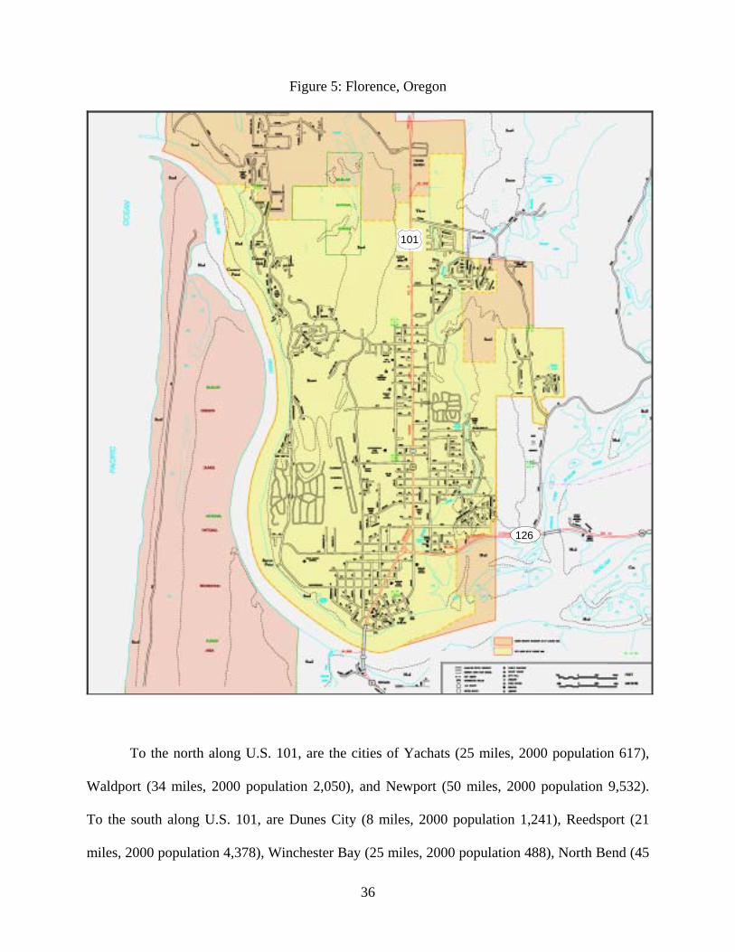
The Florence area is quite compact, with the city of Florence comprising a total area of

less than five square miles (Figure 5). Florence has two major highway connections, including

U.S. Highway 101 and Oregon Route 126. Highway 101 connects Florence with the entire

length of the Oregon coast.

12 Lane County constitutes the entire Eugene-Springfield metropolitan area.

36

Figure 5: Florence, Oregon

To the north along U.S. 101, are the cities of Yachats (25 miles, 2000 population 617),

Waldport (34 miles, 2000 population 2,050), and Newport (50 miles, 2000 population 9,532).

To the south along U.S. 101, are Dunes City (8 miles, 2000 population 1,241), Reedsport (21

miles, 2000 population 4,378), Winchester Bay (25 miles, 2000 population 488), North Bend (45

101

126

37

miles, 2000 population 9,544) and Coos Bay (48 miles, 2000 population 15,374). To the east

along Oregon 126, lies a series of small population clusters, including Cushman, Tieman,

Mapleton, and Swisshome. These areas are not incorporated cities or census designated places,

so determining the exact population is not possible using census data. Under optimal

conditions, travel in any direction can be difficult and slow due to the winding nature of the

roads. In addition, during the summer heavy tourist traffic further slows travel, especially along

Highway 101. During the rest of the year, weather conditions (rain and fog) and the threat of

rock or mudslides can make travel unpredictable. Snow and ice can occur in the higher

elevations of the Coast range along Highway 126.

The communities to the north of Florence (Yachats, Waldport, and Newport) are

experiencing population growth as well, though none as fast as Florence in percentage terms. In

addition, these communities have significant tourism industries and possess significant

concentrations of seasonal (vacation) homes. Again, this is quite similar to Florence. The

Yachats area has an especially large concentration of vacation homes. In all of these

communities, except Florence, the percentage of housing units that are classified as vacation or

seasonal homes increased between 1990 and 2000. Even though there was a small decrease in

vacation homes between 1990 and 2000 in Florence, the percentage of housing units classified as

seasonal (7.2 percent) in the 2000 census was significantly above the U.S. average of 3.1 percent.

Although tourism is important to the economy in the Florence area, the city and the nearby

region depends heavily on the timber and wood products industries.

To the south, Reedsport experienced a population increase of 18.3 percent during the

1990s, while Coos Bay and North Bend experienced virtually no population growth during this

period. The communities to the south of Florence are more dependent on natural resources

38

(mostly logging and fishing) for their economic base and do not possess the same number of

seasonal homes as the communities to their north.

Demographically, the area contains mostly whites (92 to 95 percent), with some scattered

Native American populations, Pacific Islanders, and Hispanic populations (about 1 percent each).

In Florence, the percentage of the population over age 65 is 38.2 percent, which is three times the

average for the United States (12.4 percent). In fact, the over 65 population in all of the coast

communities discussed here is above average, with the largest senior populations in Florence,

Reedsport, Winchester Bay, and Yachats and the smallest in North Bend and Coos Bay. This

reflects the attraction of the central Oregon coast area for retirees. Finally, the percent under the

poverty line is about 14.5 percent for Lane County as a whole, but 19.8 percent in Florence.13

Generally, the poverty rates in communities on the central Oregon coast are higher than the

average for Lane County,14 the exceptions being Dunes City, Yachats, and Newport.

Institutional Home for Transit Planning

Transit-planning activities for the Florence area began in 1999 and were coordinated by

the Lane Council of Governments (LCOG). Three LCOG staff members worked on this project,

providing project management, technical assistance, and GIS analysis. The initial impetus for

this activity was provided in 1998 by a $44,000 grant awarded through the Oregon Department

of Transportation’s Public Transit Division. The Lane Council of Governments provided

additional support for the project.

13 Data are from the 1990 Census and based on 1989 income. At the time of writing this report, poverty and income data from the 2000 census had not been released for individual cities and counties. 14 The poverty rate in Lane County is higher than the 1990 poverty rate for Oregon of 12.4 percent.

39

The initial focus was on the design and implementation of a localized transportation

service to operate within the City of Florence, and perhaps, if funding permitted, to serve areas

just beyond the city limits of Florence. The city was already served by a taxi voucher service

(funded under a federal 5311 operation grant) targeted specifically to senior and disabled

persons. However, the service was over-subscribed and limited to the target population. The

goal was to increase capacity and to open the service to the general public.15

Although LCOG coordinated the transit planning effort, input and assistance was

provided by the city of Florence’s planner and by the local transit steering committee. The

steering committee included representatives from the City of Florence, members of the city’s

transportation advisory committee, the local taxi provider, and other interested parties.

Invitations to participate in the planning process were sent to various social services agencies,

the local chamber of commerce, various merchants, medical and educational providers. In

addition, a community open house was held during the planning process to solicit further input.

Finally, the group made two presentations to the Florence City Council.

The initial plan for service provision was to provide a flexible fixed route system,

operating three days per week (Monday, Wednesday, and Friday). Based on this limited

availability, the initial focus had to be on non-work related trips. The system would operate on a

different route system each of the three days, but would stop at key destinations on each day.

Thus, the bus would collect passengers in a different neighborhood zone on each of three service

days, but then would deliver passengers to major retail, medical, and social service agencies on

all service days. The route system would be flexible in that passengers could ask the driver to

deviate up two blocks from the standard route in order to increase the potential for door-to-door

15 Indeed, the federal grant required that the service be opened to the general public.

40

services. Passengers with special needs (e.g. disabled) could also request home pick-ups. The

geographic scope of service would be within the city limits of Florence. Service delivery began

in the fall of 2000 and was expanded to five days per week in the summer of 2001.

Data and Analysis

The planning process in Florence involved the acquisition of significant amounts of data

covering transit demand, clients of social service agencies, and existing transit services. The

data arrived in a variety of formats, mostly electronic. Extensive review of data files was

conducted to insure accuracy and to remove duplicate records. In addition, analysts were careful

to choose only appropriate records based on fields such as case status. Generally, data that were

available at the address level were successfully converted to standard geocodes. However,

assigning geographic codes (geocoding) proved difficult in some cases due to the prevalence of

post office boxes and other addresses that were not represented in standard geocoding database

packages. The data analysts also were extremely careful to insure that confidential data would

not be inadvertently released. Consequently, many of the analytical products (e.g. maps) were

not released publicly, but rather were used “in-house” to support the analysis.16

With the focus on seniors, disabled persons, and non-working low-income persons, the

data sets shown in Table 2 were employed to measure transit demand.

16 The main reason was that the relatively small sample sizes coupled with extremely detailed maps made it potentially possible to identify specific individuals.

41

Table 2: Data types and sources Data Set Source Taxi voucher program. The existing taxi voucher program provided

invaluable data on actual origins and destinations of clients

TANF data Department of Adult and Family Services Individual level records were provided and included the home address of each client

Oregon Access Oregon Department of Human Resources National Aging Program Information System (NAPIS)

Oregon Department of Human Resources, Senior and Disabled Services provided these data. This database tracks the usage of various social services by the senior and disabled population.

Medicaid Ride Transportation database Department of Adult and Family Services HACSA housing sites Lane County Lane County Foster homes Lane County Lane County Meal sites Lane County Senior and Disabled Services Office locations

Lane County

Nursing homes, Medical offices, and hospitals

Various sources

Retail stores, especially grocery stores Various sources

Noticeably absent from the list of data sources are data sets relating to employment

locations and related activities such as employment training and child care locations. Early in

the process, the determination was made to focus on providing service for senior and disabled

persons that could also be provided to the general public. Initially the proposed service was

three days a week, which would not support a daily commute to work, school, or employment

training center. Thus, the decision was made to limit the assessment of transit to non-work

related trips. The primary focus was on activities such as shopping, medical appointments, visits

to senior centers and other social service agencies. Given that the service has since been

expanded to five days per week, it would be interesting to determine if the service could support

daily commute trips for work, educational, or training purposes.

42

Technical support for data manipulation and GIS analysis was provided by LCOG, which

already possessed much of the necessary GIS infrastructure (hardware and software) and

expertise to support the project. Funding for the planning project supported the acquisition of

additional GIS data required for the project. The GIS data analysis consisted of the development

of detailed information on potential transit demand. This was facilitated through use of

techniques such as buffer analysis to determine walking-distance catchment areas. In addition,

the transit demand analysis was used to create detailed plans for service provision, including the

proposed route structure, transit stops and check points, and identification of potential

destinations. Finally, the GIS analysis was also used to provide information about potential

ridership in areas outside of the Florence city boundaries.17

Discussion

This section describes some of the more important issues that emerged in the case studies

of transit planning in rural Oregon. First, in each case a single organization took the lead in

coordinating transit planning. In addition, a single agency emerged as a technical leader for the

provision of GIS services. From the case studies, it is clear that these organizations need not be

the same. However, having some GIS capacity within the region might be important. Finally,

for both sites it appears that the relevant data sets and GIS base layers were not readily available.

Much effort and expense was expended in order to acquire the relevant data sets and base maps.

In addition, not much attention was given to the process of continuously updating data sets to

support future analyses.

17 See the City of Florence Transit Plan (2001) for transit system details.

43

An important issue for the early stages of rural transit planning is how to determine the

relevant study area. Early in the process a decision must be made a regarding the geographic

scope of data to be collected. The decision has asymmetric implications for the geographical

focus of eventual service provision. For example, if data are collected countywide, later it will

be possible to determine the relevant service focus for any geographic subset of the county.

However, if data are initially collected for one or more cities, it will later be difficult for policy

makers to enlarge the geographic focus. Thus, the initial decision regarding the analysis area is

an important one. While selection of a particular area does not logically preclude providing

service to a larger region, it will almost certainly set a practical limit on the scope of planning

and analysis for future service provision.

Often this initial decision is based on technical considerations related to data collection or

to the political scope of the participating agencies. Both of these factors came into play in

Central Oregon. The three-county area was convenient for data collection and corresponded

nicely with the service area of the lead agency (COIC). The other collaborating institutions were

geographic sub-sets of the three-county region.

The decision about the relevant service area is tied to the issue of whether service is

provided within or between cities. For example, is the goal to transport people within the city of

Florence, or between Florence and Eugene or Newport? Similarly, Central Oregon might focus

on moving people within the city of Bend, or instead might choose to focus on moving people

from smaller cities (Redmond, Sisters, La Pine) to Bend. In the case of Central Oregon, there is

a large geographic region where the labor markets of at least some of the sub-regions may or

may not be economically integrated with the larger region.

This decision about the relevant service area is also tied to the intended client-base of the

service. For example, if the service is intended to serve seniors and disabled, then an analysis of

44

shopping trips and medically related trips is obviously appropriate. This type of service would

have a different geographic focus than work-related transit service. Thus, attention to

differences in the origins and destinations among various categories of transit demand is

important. For example, there may not be much work-related travel (even by auto) between

Sisters and Bend. But labor markets in Bend and Redmond may be linked.

Finally, it appears that one of the most important roles for GIS is to facilitate the

presentation of data in an easy to understand format. Almost always, project planners have cited

this as central to building community support for the project and to envision potential transit

service provision. Relatively sophisticated analyses of data and comparison of transit access

under alternative scenarios are rare. This may be due to the difficulty in getting the necessary

data and base maps in place. In addition, the GIS expertise necessary to support more

sophisticated analyses is likely to be beyond the reach of many rural governments.

V. ROLE OF GIS

Many agencies and jurisdictions are seeing the usefulness of mapping the locations of

low-income persons on public assistance, job locations, day-care centers, schools, and job

training sites. At the same time, few have been able to convert this information to quantifiable

terms to assist service planning and evaluation. Visual inspection of maps can be quite

subjective. A GIS-based tool can be useful for mapping this information and translating it into

measures of transportation supply and demand relative to needs of a targeted population.

Visualizing transportation networks, especially involving multiple modes is very

cumbersome in a non-graphic environment. A zonal trip time/distance matrix by mode can be

constructed, however, without an explicit spatial element. On the other hand, a (geo)graphical

map that defines network topology is not only more easily interpreted in geographic space, but it

45

also clarifies the relationships between the transportation network and surrounding activities

such as population densities, employment locations, and land use patterns. These activities are

factors in dictating not only the level of transportation demand, but also the spatial distribution of

movement, as well as the modal requirements of transportation demand. The spatial

arrangement of transportation supply and demand of transportation facilities are perfectly suited

for a GIS environment for visualization purposes and also for the data management requirements

associated with both demand and supply characteristics.

Role of GIS in Transportation Modeling Efforts

Transportation demand analysis has been greatly enhanced by the use of GIS. Using

travel demand characteristics such as population, employment, and land use, “what-if” scenarios

can be tested (Ralston, Tharaken and Liu 1994). The graphical, map-based interface provided by

GIS enhances data input and management capabilities. GIS data aggregation functions can be

used to easily assign demand characteristics to nodes on a transportation network.

Other uses of GIS for transportation modeling include traffic analysis zone and

transportation network generation. Polygon analysis (overlay and buffer) can help to determine

optimal zone sizes and geography. Two objectives of traffic analysis zone construction are

homogeneity and contiguity, which can be easily tested with a GIS (Ding 1994; Bennion and

O’Neill 1994). When zones define areas that exhibit homogenous household and land use

characteristics, transportation demand can be more effectively predicted. In addition, the

network topology capabilities of GIS assist in transportation network preparation.

46

GIS and Economic Activity

Regional economic modeling has been traditionally carried out with limited spatial

specificity. Economic characteristics for each geographic unit (region, state, county, MSA, city,

etc.) along with the likelihood of each region to interact with other regions, are the foundation for

analysis. Conceptually this can be structured in a matrix format, where geographic space does

not need to be represented realistically (i.e., in map form). Instead, cells of the matrix signify

discreet geographic units and the attribute data provide economic, social, and spatial definition.

Although such a model includes a “distance decay” factor for spatial interaction, the distance

measure is commonly a straight-line distance or average travel time or distance by a single mode

along a fixed route or shortest path. The optimization of travel routes or transportation facility

usage levels do not have a high level of importance in the modeling process. In other words,

once a balanced system of travel is achieved by the model, the model does not continue

reallocating trips to achieve a greater level of efficiency. Transportation modelers predict

movement patterns and economic modelers predict levels of economic activity. The

convergence of these two efforts could produce a valuable, integrated analytic tool. There are

few published examples of GIS applications for regional economic analysis that consider

transportation infrastructure. The following is a brief summary of three examples.

Brooks, London, Henry, and Singletary (1993) employed GIS to analyze the impacts of

infrastructure investments on employment and income distribution. In the case of transportation

investments, the GIS was used to calculate highway density measures for each of the Census

County Divisions (CCDs) in the state of South Carolina. Their results suggested that highway

accessibility has a significant impact on employment levels. An input-output (IO) table was then

used to estimate employment impacts related to output and income effects. The resulting model

47

could then be used to simulate the impacts of proposed highway improvements on employment

and industrial output.

In 1994, Hartgen and Li reported about the use of GIS for transportation corridor analysis

in a 10-county rural area of North Carolina. Their research estimated the growth impacts of

interstate exits following improvements to the roadway. They also analyzed the impacts that

resulted from decreasing travel times from manufacturers to shipping ports and also for changes

in commuter sheds because of increased accessibility. Using the GIS they were able to generate

forecasts of travel volumes which then impacted assignments. Their analysis, however, did not

consider multiple mode choice opportunities (Hartgen and Li 1994).

In a third article, Nyerges (1995) provided a thorough description of the transportation

modeling process which accounted for region-wide population, employment, and household

forecasts within a multimodal framework. He described GIS support for travel demand

forecasting in the Puget Sound Region of Washington. As is common to the demand forecasting

process, the assignments and mode choice were iterative; however, the economic impacts to the

region had no explicit feedback function to the regional demand element. Exogenous forecasts

for employment and residential growth were supplied at the traffic analysis zone level.

Unfortunately there are few, if any, examples of GIS being applied at smaller geographic

scales for transit system design or evaluation. The previous examples involved relatively

sophisticated economic and transport modeling with significant data requirements. It is unlikely

that rural transit planning efforts will have the resources to create or maintain these types of data

management systems. Therefore, an effective modeling framework for rural areas would need to

have relatively simple structure without the need for substantial data manipulation and overly

complex analytical methods.

48

GIS Tools - Accessibility, Gravity Models, and Spatial Interaction

The measurement of accessibility can take on a variety of operational forms - based upon

assumptions of the attraction between origins and destinations (gravity) and ease of movement

through space or a transportation network. One of the most fundamental forms is referred to as

"relative accessibility," where the distance or cost that separates two locations is an indicator for

the potential of interaction (Pirie 1979). A distance measure to a downtown or other central

location is an example of this. If a set of points or locations are all potential origins or

destinations, an "integral accessibility" index measures the degree of interconnection of a

location i to all other locations, j :

Ai = ijj

na

=∑

1

where Ai = integral accessibility and aij = relative accessibility (Ingram 1971). The point with

the lowest accessibility index (shortest overall distance to all other points) is most accessible and

also most central (Garrison 1968).

Relative and integral accessibility do not explicitly account for variable supply and demand

characteristics within a set of travel origins and destinations. In general, there are few situations

where trip origins are unlimited from a location and few destinations have unlimited capacities as

trip ends. Gravity models are examples of accessibility measures that are able to account for

attraction, opportunity, or capacity among points as well as distance and/or cost of travel

(Rietveld 1989). For instance;

Iij = k Xi Yj f(cij)

where interaction Iij between locations i and j is assumed to depend on conditions at i and j as

well as on interaction costs cij, Xi is a measure of the propensity of i to generate interaction and

49

Yj is a measure of the propensity of j to attract interaction; and k equals an empirically derived

constant. Xi and Yj can represent production-attraction constraints which are most frequently

used in transportation planning models. Singly or doubly constrained models can be dynamic,

reflecting changing supply or demand conditions of locations over time (Weibull 1976).

Constrained models balance trip productions and attractions so that total zonal outflows and

inflows are equal.

Each of these types of accessibility analysis methods are available within a GIS or can be

constructed as with a script or automated routine (Slavin 1996). The distance or travel time

between each location influence the level of potential interaction between two or more locations.

VI. RURAL PUBLIC TRANSPORTATION ACCESSIBILITY MODEL

Drawing upon some of the previously discussed approaches to analyzing transportation

demand, the following describes the process of constructing a model to evaluate accessibility

levels provided by a transit system. In addition, the framework can be used to compare system

configurations by means of a quantitative assessment. The framework is then applied to three

locations as a practical example of how the framework performs – “Rhody Express” transit

service in the City of Florence, the Tillamook County Transportation District, and the Bend-

Redmond Shuttle in Deschutes County. This will be followed by a discussion of framework

limitations.

50

Steps in the Model

The framework is comprised of five steps. Each of these is described, and where

possible, accompanied by an illustrative example of the procedure. Further illustration of the

process is also provided in the Florence example.

Step One. Define service area boundaries.

The geographic area to be served by transportation services should first be defined. This

should include areas with reasonable demand densities and an appropriate geographic extent to

include areas that are socially and economically linked. In addition, it should be feasible to

coordinate service provision activities within the defined area. The process of defining service

areas may initially include the use of existing administrative or physical boundaries. These can

include census geography (block groups and tracts), zip codes, school districts, or other

geographic boundaries. Ideally, all locational data for origins and destinations will be address-

based point data; however, additional aggregate characteristics will provide useful information

regarding potential service configurations. Examples of this type of information include density

measures for population, employment, and other demographic characteristics that may influence

travel activities. When aggregate data are being used, consideration should be given to

appropriate methods to disaggregate data from larger to smaller zones. For example, this

includes conflating data between boundaries that do not correspond such as census tract data to

synthetic grid-based zones. The approach does not require standard origin-destination (O-D)

data because of the expense associated with its collection and analysis. The intent was to

produce a model that maximized the use of secondary data available from state, county, and local

agencies.

51

At this stage it is also important to define reasonable service area densities within the

context of the potential transit mode that could be feasibly implemented. This could be

represented by a hierarchical scale ranging from fixed route (bus/shuttle) service for high

densities to demand responsive or subscription service for low densities. The type of transit

should also be related to the type of demand. For example, there will be a difference in the

frequency and capacity of service needed for work trips versus shopping trips. This should also

be considered for other trip types such as school, childcare, medical, and

recreation/entertainment. Another consideration is the type of client that needs transit service.

Service targeting welfare-to-work objectives implies more frequent support for the journey to

work compared to service for seniors and disabled persons.

While residents of outlying rural areas have travel needs to rural communities or centers,

there are also regional travel considerations. These regional travel needs, especially for

employment purposes, are difficult to incorporate into small-scale transit service analyses. In

terms of regional connections, however, it is important to identify nodes that represent either

travel destinations or connections to regional transportation nodes for inter-city travel. For the

purposes of this framework, the focus is on transit connections oriented to the city for

employment, commercial opportunities, and other services. This means that while regional

connections are obviously important for local transportation mobility, local travel needs are

given a priority in meeting the needs of low-income persons, seniors, and disabled persons.

Step Two. Map appropriate origins and destinations of targeted population.

This step assumes that each transportation planning agency has access to the appropriate

locational data for public assistance clients, job openings, childcare centers, schools, services,

and job training locations (see Tables 1 and 2). The data will need to be geocoded with accurate

52

base map information, including the street network and current transit service routes and stops.

Address geocoding can often be a time-consuming and expensive process, especially in urban

areas where there are large numbers of potential travel origins and destinations. For rural areas,

the task of geocoding may not be as onerous, where significantly smaller numbers of locations

need to be mapped. However, it is often more difficult to have complete and accurate

information within street network files for rural areas compared to urban areas (Drummond

1995). In addition, a system should be devised for maintaining and updating databases for

subsequent planning analyses.

The most common sources for mapping data are state and local government. State

government agencies maintain records on employers, licensed childcare providers, and job

training programs. Local agencies, especially those using GIS, can provide base map

information for streets and other land uses. Parcel databases are very useful for base maps to

show existing land use patterns. Often these databases are not available for small, rural

jurisdictions; however, the availability is increasing as more city and county jurisdictions

increase the sophistication of their GIS activities. Table 3 summarizes the data types and sources

for transit-planning activities for persons with low levels of transportation mobility (adapted

from Tables 1 and 2).

Nearly all of the data shown in Table 3 can be used as point locations based on street

address geocoding. The only exception will likely be the transit information where stops are not

typically associated with street addresses and may be located at street intersections. The result of

mapping these locations shows the geographic distribution of potential travel demand and

patterns for the selected population.

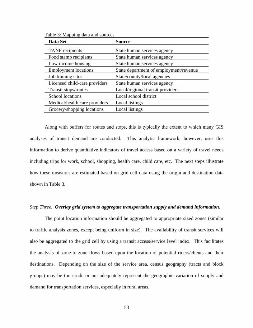
53

Table 3: Mapping data and sources Data Set Source

TANF recipients State human services agency Food stamp recipients State human services agency Low income housing State human services agency Employment locations State department of employment/revenue Job training sites State/county/local agencies Licensed child-care providers State human services agency Transit stops/routes Local/regional transit providers School locations Local school district Medical/health care providers Local listings Grocery/shopping locations Local listings

Along with buffers for routes and stops, this is typically the extent to which many GIS

analyses of transit demand are conducted. This analytic framework, however, uses this

information to derive quantitative indicators of travel access based on a variety of travel needs

including trips for work, school, shopping, health care, child care, etc. The next steps illustrate

how these measures are estimated based on grid cell data using the origin and destination data

shown in Table 3.

Step Three. Overlay grid system to aggregate transportation supply and demand information.

The point location information should be aggregated to appropriate sized zones (similar

to traffic analysis zones, except being uniform in size). The availability of transit services will

also be aggregated to the grid cell by using a transit access/service level index. This facilitates

the analysis of zone-to-zone flows based upon the location of potential riders/clients and their

destinations. Depending on the size of the service area, census geography (tracts and block

groups) may be too crude or not adequately represent the geographic variation of supply and

demand for transportation services, especially in rural areas.

54

The purpose for using grid cells is to control the geographic resolution of the previously

discussed data. Using only point location data makes it difficult to generalize travel demand

patterns (see Figure 6). In addition, relying on existing geographic zone boundaries like census

tracts or block groups produces distorted maps that can be difficult to interpret due to the

irregular geometry of census geography. Grids can be easily generated using scripts or macros

within most desktop GIS programs (e.g., Avenue scripts are available for use within ArcView

3.X). For rural areas, tracts or block groups can tend to be large and not depict sufficient detail

at a local scale.

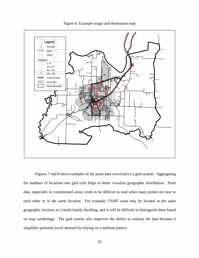
55

Figure 6: Example origin and destination map

%

%% %

%%

%

%%

%% % %%%%%%% %%%%% %% % %%% %% %%%%%%% %%%%%%% %% %%% %%%% % %%% %%% %% % %% %%%% %%% % %% %

%%

%

; ; ;

; ;

d

d

d

dd dd

dd

d

d d

dddd

d

dddd

d

d

ddd

dd

d

d

T a n f c a s e s d S t r e e t s S c h o o l s ;

E m p l o y e r s 1 - 1 0 % 1 0 . 1 - 2 0 % 2 0 . 1 - 1 0 0 % 1 0 0 . 1 - 2 2 5 %

T r i - M e t b u s r o u t e s C i t y o f C a n b y S t u d y a r e a b o u n da r y

L e g e n d

Figures 7 and 8 show examples of the point data converted to a grid system. Aggregating

the numbers of locations into grid cells helps to better visualize geographic distribution. Point

data, especially in concentrated areas, tends to be difficult to read when many points are near to

each other or in the same location. For example, TANF cases may be located in the same

geographic location as a multi-family dwelling, and it will be difficult to distinguish them based

on map symbology. The grid system also improves the ability to analyze the data because it

simplifies potential travel demand by relying on a uniform pattern.

56

Figure 7: Gridded employment map

Study ar ea boundary

Tri-Met bus routes

Streets

Employment0

1 - 10

11 - 25

26 - 50

51 - 300

Legend

57

Figure 8: Gridded TANF recipient locations

Study area boundary

Tri-Met bus routes

Streets

TANF Cases0

1 - 5

6 - 10

Legend

The availability of transit services within each grid cell can be coded in regard to access

to the nearest route/stop and level of service. While a route may not run directly through a cell, a

cell may still be within walking distance and should be counted as having transit access.

Typically distances of less than one-quarter mile are considered reasonable for walking access to

transit. Cells can either be coded as being within this distance or actual distances can be used as

a continuous measurement. Additional information can be used for more specific indicators of

service level or quality. For example, the average service frequency (number of stops per hour,

day, or week) and/or cost can be assigned to each cell. The next section discusses how zones can

be analyzed to determine levels of transit accessibility.

58

Step Four. Analysis of transit supply and demand characteristics.

Accessibility measures can be generated from the data shown in the previous two steps.

The objective is to calculate quantifiable measures that indicate the overall level of accessibility

being provided by local transit services. The basis of the measure discussed here is a simple

gravity model, modified to account for differential weighting of destination types and expected

levels of travel demand. The example includes an ArcView Avenue script to calculate a

gravity/accessibility measure for each grid cell (see Appendix B). A grid cell score can then be

assigned to individual client locations, with the average score for clients being the overall system

score. Alternative scenarios can be evaluated by comparing the mean values of these scores

(discussed in the next section on performance evaluation).

As previously mentioned, a gravity type measure is used to estimate accessibility levels

for each grid cell based on the attractiveness of locations within each cell. The measure also

takes into account whether transit service is available at the origin cell and the destination cell.

The formula would look something like the following:

Ai = ∑=

⋅+⋅⋅⋅n

j ij

jjji

DSWTT

12

))028.0()107.0(()(

where:

Ai = the accessibility of grid cell i iT = transit service in grid cell i (binary)

jT = transit service in grid cell j (binary) jW = number of jobs located in grid cell j

jS = number of schools in grid cell j D ij = euclidean distance from grid cell i to grid cell j

In a full model, the other potential destinations shown in Table 3 should also be included.

Job locations ( jW ) should include only those that represent a relatively close match to the job

59

skill and educational levels of potential riders. In the case of TANF recipients, these tend to be

jobs in the service, retail, and manufacturing industries. These jobs can be isolated from the

employment data using the appropriate two or three digit standard industrial classification code

(SIC). The trip weights shown in the equation can be modified based on local or regional travel

survey data. Otherwise, national survey data is available from the Nationwide Personal

Transportation Survey (NPTS) that shows trip frequency by income level, trip purpose, and

travel mode. For this example, transit trips for low-income persons living in non-urban areas

were used. Trip purpose weights derived from NPTS data are shown in Table 4. As can be seen,

weights vary depending on trip purpose and income level.

Table 4: Example trip purpose weights derived from 1995 NPTS data Low Middle High

Trip Purpose Income Income Income Total

Work 10.7% 14.7% 16.8% 14.0% Shopping 14.6% 12.7% 12.5% 13.1% School 2.8% 3.7% 2.9% 3.3% Medical 1.1% 0.8% 0.6% 0.9% Recreation 0.1% 0.2% 0.3% 0.2% Other 70.7% 67.8% 67.0% 68.5%

The script can be modified to prompt the user for trip purpose weights, or they can be

hard-coded within the script and modified as needed by the GIS analyst. In addition, the distance

decay exponent (shown as 2 in the example above) can also be modified by user input or hard-

coded into the script. The exponent on the distance variable in the denominator affects the

attraction between locations as the travel distance between them increases (see Sheppard 1984

for a discussion of distance decay factors). As can be seen in the formula, the interaction

between cells is also a function of whether transit service is within 0.25 miles of origin and

destination grid cell centroids. This is obviously a simplified indicator of accessibility because it

60

is not based on actual network connectivity, but rather the assumption that routes in a local

transit network are completely interconnected. In addition, it also assumes that there is a

significant correlation between the straight-line distance and actual network distance between

cells. The model can include network distances between cells if a more sophisticated model is

desired. Depending on the scale of the planning area, network distances may not significantly

impact model results.

Sample output from the gravity model is shown in Figures 9 and 10. These maps show

that having physical access to transit is beneficial, however, being close to important travel

destinations also has positive impacts. Figure 9 shows an example of current transit routes and

Figure 10 shows increased service levels resulting from route additions. The next section will

discuss the comparison of accessibility scores between these two scenarios.

61

Figure 9: Gravity model output for existing conditions

Study area boundary

Tri-Met bus routes

Streets

AccessibilityLow

Medium

High

Highest

None

Legend

Figure 10: Gravity model output for proposed transit system

Study area boundary

Canby bus routes

Streets

AccessibilityLow

Medium

High

Highest

None

Legend

62

Step Five. Performance evaluation.

As mentioned earlier, each potential rider/client is assigned the accessibility score for the

grid cell in which they reside. The average accessibility score for all riders/clients in the

planning area then becomes the overall score for a particular service plan or route configuration.

The aggregate scores for different service scenarios can be compared to indicate the magnitude

of increase or decrease in accessibility. For the two examples shown in Figure 9 and Figure 10,

the accessibility score was 333.4 in the first and 336.2 in the second. This represents less than a

1 percent increase in average transit accessibility for TANF cases within the selected service area

(and a 14 percent increase for all grid cells). The scores can be used as relative measures for

monitoring or evaluation purposes because the absolute scores are not easily interpreted in

common units. Depending on the weighting system used, the accessibility measure is essentially

the average number of opportunities that can be reached per unit of distance (accounting for

declining attraction as distance increases).

Given the use of a gravity-type model, it can be seen that accessibility levels can be

increased not only by providing more transit service, but also through the location of

employment and other locations that need to be reached by transit. It is important also to account

for external transit connections because these locations (such as employment centers) may serve

multiple areas due to overlapping commuting sheds.

Baseline information for the service area is important, to be able to evaluate the outcomes

of new service provision. Ideally, baseline information will be collected prior to any service

improvements or changes. This includes not only the types and quality of transit service being

offered, but also information about origins (i.e., riders/clients) and destinations (i.e., employment

locations) as discussed previously. A comparison of system performance should take into

account residential and employer relocations, because they influence the spatial pattern of

63

demand for transportation services. These transportation supply and demand measurements can

be used to detect net changes in mobility needs within the service area. The model can also be

used to evaluate service-planning scenarios both in terms of transportation service delivery and

employment access. New routes/stops can be mapped to estimate the effect on transit and

employment accessibility.

City of Florence, Rhody Express Example

The previous modeling framework was applied to the City of Florence to compare the

levels of transit access provided with an initial service route versus a modified route

configuration. The newer (expanded) route was a response to perceived gaps in service and

represented an effort to provide greater coverage within the City of Florence. The following is a

brief summary of the model results for Florence.

Step One. Define service area boundaries.

The Rhody Express only serves the City of Florence and is reasonably self-contained.

For this reason the incorporated limits of Florence was used as the service area boundary.

Step Two. Map appropriate origins and destinations of targeted population.

The residential locations of low-income persons receiving public assistance (TANF

recipients) were address-geocoded along with the locations of local employment. There were

107 residential locations and 46 employment locations (approximately 230 jobs) mapped.

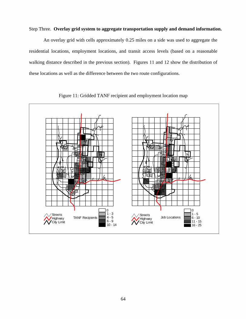
64

Step Three. Overlay grid system to aggregate transportation supply and demand information.

An overlay grid with cells approximately 0.25 miles on a side was used to aggregate the

residential locations, employment locations, and transit access levels (based on a reasonable

walking distance described in the previous section). Figures 11 and 12 show the distribution of

these locations as well as the difference between the two route configurations.

Figure 11: Gridded TANF recipient and employment location map

TANF RecipientsCity LimitHighwayStreets

City LimitHighwayStreets

Job Locations1 - 34 - 56 - 910 - 14

01 - 56 - 1011 - 1516 - 25

0

65

Figure 12: Transit service route maps

Current Route

Initial Route

Step Four. Analysis of transit supply and demand characteristics.

The gravity model discussed in the previous section was applied to the grid cell data for

the City of Florence using the trip weights shown in Table 4.

Step Five. Performance evaluation.

The total transit accessibility score for the initial Rhody Express route was 2,426.4 (12.6

average per grid cell). The score improved to 2,802.9 (14.6 average per grid cell) an increase of

15.5 percent. The scores also increased on average for the low-income residences included in

66

the analysis. The average transit accessibility score for these locations was 45.4 with the initial

route and 57.6 for the expanded route, an increase of 26.9 percent. Not only did the new route

increase transit access generally for the City, but it also represented significant increases for

persons most likely to have low levels of transportation mobility (i.e., automobile access). The

accessibility measure generated by this framework should be validated by other measures of

service effectiveness. These other measures may include economic cost and benefit analyses,

actual ridership, and user surveys. User input should not only be utilized in evaluation phases,

but also in initial system planning phases (Schauer 1992).

Tillamook County Transportation District Example

Compared to the City of Florence example, the Tillamook County system is much larger

in scale, both in terms of geography and transit system coverage (see Figure 13). However, the

same approach was applied to evaluate the level of transit/employment access for the current

system within the county. Unlike Florence, alternative route configurations were not tested –

only the existing routes. Instead, general accessibility levels were compared to those for low-

income residents to assess the effectiveness of the system in meeting their mobility needs.

The total transit accessibility score for the Tillamook County system was 374.2 (the

average score per grid cell was 0.52). The scores are relative measures and cannot be compared

across jurisdictions due to differences in geographic scale. For example, the City of Florence

had an average of 14.6 per grid cell – but this does not mean that accessibility levels are

necessarily 28 times higher in Florence, rather, the higher levels of accessibility are also a

function of the total geographic areas being analyze (which is much smaller in the case of

Florence compared to Tillamook County). The transit accessibility score was higher for low-

income persons averaging 4.66 compared to general accessibility levels.

67

Figure 13: Tillamook County Transportation District

Bend-Redmond Shuttle Example

A third example of the transit accessibility model was applied to the Bend-Redmond area.

A shuttle program was proposed by the Central Oregon Intergovernmental Council (COIC) that

would not only link Bend and Redmond, but also provide limited internal circulation in both

cities. The system was not yet operational at the time, so the analysis showed how the model

68

could be used in the planning stages of a transit system. The model was used to evaluate, a) the

Bend-Redmond segment, b) the Bend Portion, and c) the entire shuttle system (see Figure 14).

Figure 14: Proposed Bend-Redmond Shuttle

The route linking Bend and Redmond resulted in an average accessibility score of 4.76

per grid cell with the Bend portion achieving a score of 4.56 (average per grid cell) separately.

As might be expected, an analysis of the whole system yielded a greater level of overall

transit/employment access (11.99 per grid cell); but it is helpful to evaluate individual route

segments to determine their relative importance compared to other segments. Again, as in the

cases of Florence and Tillamook, the proposed shuttle routes provided a higher level of transit

69

accessibility for low-income residents with an average accessibility score of 37.12. This score is

over eight times higher than the general accessibility score, as compared to approximately four

times higher in Florence and nine times higher in Tillamook.

Model Limitations

One objective of this project was to illustrate the utility of a relatively simple GIS-based

tool for rural transit planning. Rural transit agencies are faced with resource constraints that

often limit staffing and access to technologies such as GIS. For this reason, it was recommended

that only available, secondary data sources be used. In addition, it was recommended that a

readily available GIS software package be used rather than a customized application requiring

extensive data manipulation and software training. The framework proposed could be utilized by

persons with rudimentary skills and some programming experience. As a result of simplifying

the data input and analysis methods (relative to typical transportation modeling techniques), the

output of the model presented here lacks the sophistication and specificity of traditional

models.18 On the other hand, it is likely that most rural transit agencies have not previously

engaged in sophisticated modeling, so this model still represents an improvement over

commonly employed methods.

VII. SUMMARY AND CONCLUSIONS

The objective of this project was to consider the nature of rural transit in the context of

both transportation and social service planning. Welfare reform policies that have emphasized

labor force participation for persons previously not working and receiving public assistance have

18 For example, using trip rate functions from national or state data may not be suitable for a particular rural area.

70

identified the importance of transportation mobility during this transition. This is especially

challenging in rural areas of the U.S. where traditional types of fixed-route transit service is very

difficult to provide.

In light of the issues faced by rural transit planning efforts, this project sought to provide

examples of how GIS is being used to meet these challenges. We learned that GIS is being used

widely for transit planning purposes, including rural areas of the country. While this technology

is being applied in rural planning efforts, it tends to occur at a relatively unsophisticated level,

however. It may be that while GIS technology has been readily adopted by urban areas, it is still

diffusing among rural jurisdictions. This adoption process is likely to continue given the

advances and increasing availability of GIS to smaller jurisdictions.

On the other hand, the general lack of GIS innovation in rural transit planning may also

be a function of scarce resources - including those needed to implement current information

technologies. In the cases of the rural Oregon transit planning activities, low levels of staff

resources along with reliance on instable (or short-term) funding sources negatively affected

organizational structure needed to support information technologies like GIS. While agencies

can quickly generate useful transit planning products using GIS, changes in staff and agency

resources can quickly shift the priorities of the agency from planning to operations activities.

This is an important consideration for rural planning agencies that may be considering an

investment in GIS technology. Strategic planning around these issues should consider multi-

agency/jurisdiction cooperation in building, maintaining, and operating GIS functions for

planning purposes to increase the viability and benefits of these investments.

It is important to consider how this analysis function could fit into the overall planning

approach and objectives of an agency. The appropriateness of this model will depend on several

factors related to how an agency plans to use the output. If the agency has only a one-time need

71

for such an analysis, it may be more efficient to have a consultant or contractor perform the

work. Or it may be more cost effective to have a larger, local agency with more resources (such

as a county government or association of governments) perform the analysis. For a one-time

analysis, developing the technical resources (especially for GIS) may not be advisable.

On the other hand, if an agency has the resources to develop a GIS and transportation

modeling capacity, the model presented here may be a reasonable first step. In this case, the

initial model results could be validated, and the model could be maintained and updated, with

on-going data collection and further modeling efforts. Based on the experience of the case

studies presented earlier in this report, however, such a modeling effort appears unlikely, because

rural planning agencies tend to rely on unstable funding sources and are not likely to have the

time and resources required to achieve sophisticated GIS and modeling capabilities.

Finally, the evaluation framework presented here represents a relatively simple method

for rural transit systems. The framework relies on a gravity model to assess transit accessibility

within a defined service area. The proposed model was intentionally simplified (compared to

traditional urban transportation planning models) because of its intended implementation by

agencies tending to have low levels of staffing and GIS resources. Using the framework

provides transit system planners with objective and quantifiable measures of service levels. This

represents an improvement over the most common GIS approaches currently being utilized by

rural transit planning agencies that rely on subjective interpretation of geographic relationships

between potential trip origins and destinations.

72

VIII. REFERENCES

Accordino, J. 1998. The Consequences of Welfare Reform for Central City Economies. Journal of the American Planning Association. Winter: 11-14.

Anderson, Larry D. 1991. “Applying Geographic Information Systems to Transportation Planning.”

Transportation Research Record 1305, 113-117. Basile, Ralph E., Thomas TenEyck, and Anthony J. Pietropola. 1991. “Geographic Information

System for the Pennsylvania Department of Transportation.” Transportation Research Record 1305, 118-122.

Bennion, Wayne M. and Wende A. O’Neill. 1994. “Building Transportation Analysis Zones using

Geographic Information System.” Transportation Research Record 1429, 49-56. Brooks, K.R., J.B. London, M.S. Henry, and L.A. Singletary. 1993. “Analysis and simulation of

employment and income impacts of infrastructure investments in a state-wide GIS framework.” Computers, Environment, and Urban Systems, 17:129-151.

Casavant, K. and Painter, K. 1998. Demand Forecasting for Rural Transit. Available from:

www.ntl.bts.gov.DOCS/ruraldemand. Central Massachusetts Regional Planning Commission. 2000. Welfare to Work: A Cooperative

Effort of CMRPC and RTA. Available from: www.cmrpc.org/welwork. Community Transportation Association of America. 2000. ITS and Smaller Transit Systems.

Available from: www.ctaa.org/ntrc/its/incert1. Davis, J.; Telovsky, W.; Vaughan, T. 1998. “Building Applications to Support the Effective Use of

GIS by NYS Transit Operators.” Available from: [email protected] Ding, Chengri. 1994. “Impact Analysis of Spatial Data Aggregation on Transportation Forecasted

Demand: A GIS Approach.” Urban and Regional Information Association, URISA, 362-375. Drummond, William. 1995. “Address Matching: GIS Technology for Mapping Human Activity

Patterns.” Journal of the American Planning Association. 61, 3: 240-251. Dueker, Kenneth J. and Ric Vrana. 1995. “Systems Integration: A Reason and a Means for Data

Sharing.” in Onsrud, Harlan J. and Gerard Rushton, eds. Sharing Geographic Information, Center for Urban Policy Research, New Brunswick, New Jersey.

Environmental Systems Research Institute. 1997. Getting to Know ArcView GIS. Cambridge:

GeoInformation International.

73

Evans, John and Joseph Ferreira, Jr. 1995. “Sharing Spatial Information in an Imperfect World: Interactions Between Technical and Organizational Issues” in Onsrud, Harlan J. and Gerard Rushton, eds. Sharing Geographic Information, Center for Urban Policy Research, New Brunswick, New Jersey.

Fawson, C., Thilmany, D. and Keith, J. 1998. Employment Stability and the Role of Sectoral

Dominance in Rural America. American Journal of Agriculture Economics. 80, 3: 521-535. Findeis, J. and Jensen, L. 1998. Employment Opportunities in Rural Areas: Implications for Poverty

in a Changing Policy Environment. American Journal of Agriculture Economics. 80, 5: 1000-1009. Fletcher, C. and Jensen, H. 2000. Transportation Needs and Welfare Reform in Rural Iowa: A Case

Study. Consumer Interests Annual. 46: 30-38. Freshwater, D. 1996. The Future of Low-Wage, Low-Skills Jobs in Rural Areas. International

Advances in Economic Research. 2, 4: 498. Garrison, William L. 1968. "Connectivity of the Interstate Highway System." in Brian J.L. Berry and

Duane F. Marble, eds. Spatial Analysis, 239-249, Prentice-Hall, Inc., New Jersey. Hartgen, David T. and Yuanjun Li. 1994. “Geographic Information Systems Applications to

Transportation Corridor Planning.” Transportation Research Record 1429, 57-66. Hartgen, David T., Yuanjun Li, and George Alexiou. 1993. “Super-Regional, Very Long Range

Transportation Modeling with a Geographic Information System.” Transportation Research Record 1413, 78-87.

Heywood, I., Cornelius, S., and Carver, S. 1998. An Introduction to Geographical Information Systems.

New York: Pearson Education Inc. Ingram, D.R. 1971. "The Concept of Accessibility: A Search for an Operational Form." Regional

Studies, 5:101-107. Johnson, S. 2001. Central Massachusetts Regional Planning Commission. Letter to the author,

February. Kaplan, A. 1997. Transportation and Welfare Reform. Welfare Information Network. 1, 4. Kihl, M., J. Knox, and T.W. Sanchez. 1997. Alternative Approaches to Providing Passenger

Transportation in Low Density Cities: The Case of Council Bluffs, Iowa, City of Council Bluffs and the Iowa Department of Transportation.

Kilkenney, M. 1998. Transit Costs and Rural Development. Journal of Regional Science. 38, 2: 293-313. Lam, W. and J. Morrall. 1982. Bus Passenger Walking Distances and Waiting Times: A Summer-

Winter Comparison. Transportation Quarterly. 36, 3: 407-421.

74

Loker, R. 2001. Assistant Director for Communications and Community Initiatives. St. Mary’s Department of Social Services. Letter to the author, July.

Marks, E. et al. 1999. Rural Welfare to Work Strategies: Research Synthesis. Macro International,

Inc. Available online: www.macroint.com/publications/synthesis.pdf. Multisystems, Inc. 2000. Transit Route Design Applications Using Geographic Information Systems.

TCRP Report 60, Washington D.C.: National Academy Press. Niemeier, Debbie A. and M. Kate Beard. 1993. “GIS and Transportation Planning: A Case Study.”

Computers, Environment, and Urban Systems, 17:31-43. Nightingale, D.S. 1997. Transportation Issues in Welfare Reform: Background Information. U.S.

Department of Labor # F-5532-5-00-80-30. Washington D.C.: The Urban Institute. Nyerges, Timothy L. 1995. “Geographic Information System Support for Urban/Regional

Transportation Analysis.” in Susan Hanson, ed. The Geography of Urban Transportation, The Guilford Press, New York.

Onsrud, Harlan J. and Gerard Rushton, eds. 1995. Sharing Geographic Information, Center for Urban

Policy Research, New Brunswick, New Jersey. Pindus, N.M. 2001. Implementing Welfare Reform in Rural Communities. U.S. Department of

Agriculture, # 43-3AEM-8-80103, Washington D.C.: The Urban Institute. Pirie, G.H. 1979. "Measuring Accessibility: A Review and Proposal." Environment and Planning A, 11:

299-312. Ralston, Bruce A., George Tharakan, and Cheng Liu. 1994. “A Spatial Decision Support System for

Transportation Policy Analysis in Bangladesh.” Journal of Transport Geography, 2(2):101-110. Ramirez, A. and Seneviratne, P. 1996. Transit Route Design Applications Using Geographic

Information Systems. Transportation Research Record, No.1557: 10-14. Rietveld, Piet. 1989. "Employment Effects of Changes in Transportation Infrastructure:

Methodological Aspects of the Gravity Model." Papers of the Regional Science Association, 66:19-30. Rural Policy Research Institute. 1998. Welfare Reform in Rural Areas. Available from:

www.rupri.org/rupolicy/P98-6/briefing. San Luis Obispo Council of Governments. 1998. Welfare Reform Mobility Study: Final Report. San

Luis Obispo County, California: Nelson & Nygaard. Schauer, P. 1992. Rural Public Transportation, in G. Gray and L.A. Hoel, (eds.) Public Transportation.

Prentice-Hall, Inc., New Jersey. Schoppert, D.W. and W.S. Herald. 1978. Pedestrian Range as Related to Transit Stations and

Immediate Surroundings. ITE Journal. 48: 13-18.

75

Sheppard, E. 1984. The Distance Decay Gravity Model Debate, in G. Gaile and C. Willmot (eds.) Spatial Statistics and Models. Dordrecht: D.Reidel.

Simkowitz, Howard J. 1990. “Integrating Geographic Information System Technology and

Transportation Models.” Transportation Research Record 1271, 44-71. Slavin, Howard. 1996. “An Integrated, Dynamic Approach to Travel Demand Forecasting.”

Transportation, 23:313-350. U.S. Census Bureau. 1990 Decennial Census -STF1. Available from: www.census.gov. U.S. Census Bureau. 2000 Decennial Census –STF1. Available from: www.census.gov. U.S. Department of Transportation, Bureau of Transportation Statistics. 1998. Welfare Reform and

Access to Jobs in Boston, BTS-98-A-02, prepared by Annalynn Lacombe, Washington, D.C. U.S. General Accounting Office. 1998. Welfare Reform: Transportation’s Role in Moving From

Welfare to Work. Report to the Chairman, Washington D.C. GAO/RCED-98- 61. Ward, B. 2000. Public Transportation and Welfare to Work: A Paper Exploring Issues of Access

and Mobility Related to the Federal Personal Responsibility and Work Opportunity Reconciliation Act of 1996. Center for Urban Transportation Research Available from: www.cutr.eng.usf.edu/index2.

Weibull, J.W. 1976. "An Axiomatic Approach to the Measurement of Accessibility." Regional Science

and Urban Economics, 6:357-379. Zarean, M., Buergler, B., Burkardt, Y., and Schweiger, C.L. 1998. Rural Public Transportation

Technologies: User Needs and Applications. FHWA-RD-98-125. Alexandria, VA. TransCore/SAIC.

76

77

IX. APPENDICES

Appendix A

RURAL MOBILITY AND GIS CASE STUDY SURVEY

Please attach additional sheets with your responses and refer to each by the question number listed below. General Agency

1. Contact person(s) and position(s) 2. Organization name 3. Geographic region of jurisdiction 4. Population size of planning area and general demographic profile Project Background

5. Describe staff resources used for the project (no. of persons, time commitment to the project, responsibilities, etc.)

6. Provide a general description of your rural transit project that uses GIS 7. Describe the primary motivation of the project (i.e., project origins) 8. How was the targeted low-income population defined and identified for your project? 9. What types of transit service are planned or provided? 10. Describe why particular types of service were chosen (e.g., van service vs. taxi vouchers) 11. How was trip demand estimated for each type of service? 12. What types of trips are being addressed (e.g., work commute, medical, shopping)? 13. List the sources of funding for the project and describe how funding was obtained 14. What is the anticipated project duration and probability of extension (or is it on-going)? 15. List the organizations involved with the project (such as governmental agencies, community/neighborhood

groups, business organizations, religious organizations, etc.) 16. Describe the primary role of these organizations (e.g., project design, data sharing, funding provider) 17. Describe project coordination among these organizations 18. Identify specific project stakeholders 19. Describe the level of public participation associated with the project (e.g., public hearings, surveys, focus

groups). Include efforts to obtain public input, approximate number of participants, format of comments. Also describe how public input shaped the project.

20. Describe the techniques that were used to solicit public input and participation

78

Aspects of GIS

21. List the types of data used, including source, geographic unit, and types of attribute information 22. Describe how this data needed to be processed before it could be used for your project (e.g. data

conversion, geocoding) 23. Describe the problems encountered with acquiring and using the data (e.g., confidentiality restrictions, data

format) 24. Describe how these data sources were identified 25. List the GIS analysis techniques used (e.g., buffer analysis, network analysis) 26. List other analysis methods used (e.g., statistical methods, demand forecasting) 27. Describe your hardware and software environment 28. Describe sources of technical assistance, consulting, and training 29. Describe the role of GIS in the project decision making process 30. Describe any uses that project partners made of the GIS maps, outside of project goals (e.g. funding

presentations, social service design discussions, service aggregation, budget hearings, etc.) 31. Describe any institutional barriers that were encountered while developing the GIS analysis Other Project Information

32. Describe the methods that will be used to evaluate project performance 33. Describe how the project may be modified as a result of performance evaluation 34. Describe how other projects may benefit from the processes and outcomes of this project 35. Describe any future plans to increase/reduce the scale of the project 36. Describe future implementation plans (e.g., Internet-based applications, custom applications) 37. List any project proposals, documentation, reference material, and reports associated with the project. Are

copies of these available? 38. Describe any notable outcomes of the project (to date) based on project evaluation as well as administrative

lessons learned 39. Provide any general comments that you think will help us to better your project Thanks again for your assistance. Please feel free to give me a call at 1-800-547-8887, ext. 8743 if you have any questions.

79

Appendix B

Avenue Script for Accessibility Calculations '----- Get the active view theView=av.GetActiveDoc '----- Build a list of fthemes from the theme list. The user will be asked to select from the list. thms=List.Make for each t in theView.GetThemes if (t.Is(Ftheme)) then shapetype = t.GetFtab.FindField("Shape").GetType if (shapetype = #FIELD_SHAPEPOINT) then thms.Add(t) end end '----- If < 1 themes are fthemes, bail out. if (thms.Count < 1) then System.Beep MsgBox.Error("There must be at least one point feature themes in the View to proceed! Exiting.","Error") exit end '----- Ask the user which theme to use as input: theInputTheme = MsgBox.Choice(thms,"Select the point theme for the distance matrix","SELECT INPUT POINT THEME") if(theInputTheme = nil) then exit end '----- Activate the attribute table of the selected point theme theInputTheme.EditTable '----- Open the coordinates table tab1 = av.GetProject.FindDoc("Attributes of "+theInputTheme.asString) '----- Get the virtual table of the coordinates table aVtab1 = tab1.GetVTab '----- Calculate the X-coord and Y-coord of each point and store it in the attribute table _theProjection = theView.GetProjection project_flag = _theProjection.IsNull.Not 'true if projected '----- get the theme table and current edit state theFTab = theInputTheme.GetFTab theFields = theFTab.GetFields edit_state = theFTab.IsEditable '----- make sure table is editable and that fields can be added if (theFtab.CanEdit) then theFTab.SetEditable(true) if ((theFTab.CanAddFields).Not) then MsgBox.Info("Can't add fields to the table."+NL+"Check write permission.", "Can't add X,Y coordinates")

80

return nil end else MsgBox.Info("Can't modify the feature table."+NL+ "Check write permission.","Can't add X,Y coordinates") return nil end '----- Check if fields named "X-coord" and Y-coord" exist x_exists = (theFTab.FindField("X-coord") = NIL).Not y_exists = (theFtab.FindField("Y-coord") = NIL).Not if (x_exists or y_exists) then if (MsgBox.YesNo("Either click Ok to overwrite and continue? Or click No to halt and check out your table for the existing values","X-coord, Y-coord fields already exist", false)) then '----- if ok to overwrite, delete the fields as they may not be defined '----- as required by this script (eg., created from another script). if (x_exists) then theFTab.RemoveFields({theFTab.FindField("X-coord")}) end if (y_exists) then theFTab.RemoveFields({theFTab.FindField("Y-coord")}) end else msgbox.error("Your current operation stopped","Alert!") return NIL '----- Skip the calculation of x-coord and y-coord... end 'if (MsgBox...) end ' if x = Field.Make ("X-coord",#FIELD_DECIMAL,18,5) y = Field.Make ("Y-coord",#FIELD_DECIMAL,18,5) theFTab.AddFields({x,y}) '----- Get point coordinates or polygon centroid coordinates if (project_flag) then 'Projection defined theFTab.Calculate("[Shape].ReturnProjected(_theProjection).GetX", x) theFTab.Calculate("[Shape].ReturnProjected(_theProjection).GetY", y) else 'No projection defined theFTab.Calculate("[Shape].GetX", x) theFTab.Calculate("[Shape].GetY", y) end 'if '----- Return editing state to pre-script running state theFTab.SetEditable(edit_state) '----- Locates the X_coord field in the coord tab afield1 = avtab1.FindField("X-coord") '----- Locates the Y_coord field in the coord tab afield2 = avtab1.FindField("Y-coord") afield3 = avtab1.FindField("Jobs") afield4 = avtab1.FindField("Schools")

81

afield5 = avtab1.FindField("Transit") '----- Select an ID field INftab = theInputTheme.getFtab theInputfields=list.make for each f in INftab.getfields if ((f.GetName = "Shape") or (f.GetName = "area") or (f.GetName = "perimeter") or (f.GetName = "Hectares") or (f.GetName = "length")) then continue else fCopy = f.Clone theInputFields.Add(fCopy) end end i= Msgbox.Choice(theInputFields,"Select the field that represents the unique IDs of the point features you want to tag your distance table with","Select the ID field") if(i = NIL) then msgbox.error("You have choose not to continue with the matrix creation or your attribute table does not have an ID for each point feature!","Alert") return NIL end '----- Verify if the selected field has unique IDs in it vr = NIL 'Initial Value '----- Loop in the records of the selected field for each rec in aVtab1 ver = aVtab1.ReturnValue(i, rec) if ((vr = ver) And (rec > 1)) then msgbox.error("The field you have selected does contain unique ID's of the point features, Please recheck your attribute table for the ID field with unique values. This operation will halt","Alert!") return NIL 'exist script else vr = ver '----- Assign value to the initial variable to check if duplicates exist in the selected field end end '----- Creates a dbase file myFile = FileDialog.Put( "gravity.dbf".asfilename, "*.dbf", "Gravity Index File Name") if (myFile = nil) then exit end theVTab = VTab.MakeNew(myFile,dbase) myTable = Table.Make(theVtab) vtab2 = myTable.GetVtab f0 = Field.Make( "IDs",#FIELD_CHAR, 10, 0 )

82

'----- Creates the first Tag column of point ids in the matrix table theVTab.AddFields( {f0} ) ' '----- declare the number of points in the original table and creates the columns of the '----- distance matrix '----- Creates a sequence of fields presenting columns in the matrix ' 'for each rc1 in aVtab1 'r = rc1 ' v = aVTab1.ReturnValue(i, rc1) f1 = Field.Make("Access",#FIELD_DECIMAL, 10, 3 ) theVTab.AddFields( {f1} ) 'end '----- Creates a sequence of records representing rows for each rec in avtab1 vtab2.AddRecord v = aVTab1.ReturnValue(i, rec) vtab2.SetValue( f0, rec, v ) theVtab.SetValue( f0, rec, v.asString) end gi = 0 for each rec in avtab1 X1 = aVTab1.ReturnValue(aField1, rec) ' This reads the X1 value of the first pt Y1 = aVTab1.ReturnValue(aField2, rec) ' This reads the Y1 value of the first pt T1 = aVtab1.ReturnValue(aField5, rec) for each rec in avtab1 Q = rec +1 X2 = aVTab1.ReturnValue(aField1, rec) ' This reads the X2 value of the second pt Y2 = aVTab1.ReturnValue(aField2, rec) ' This reads the Y2 value of the second pt W2 = aVTab1.ReturnValue(aField3, rec) ' This reads the attractiveness field for second pt S2 = aVTab1.ReturnValue(aField4, rec) ' Reads the schools number in second location T2 = aVTab1.ReturnValue(aField5, rec) ' Reads transit availability in second location arg = ((Y2 - Y1)*(Y2 - Y1)) + ((X2 - X1)*(X2 - X1)) 'Calculates the argument of the distance d = arg.sqrt / 5280 'Calculates the distance between two points if (d > 0) then g = (T1 * T2) * (((W2 * 0.107) + (S2 * 0.028))) * (1 / d ^ 2) gi = g + gi else g = 0 end 'MsgBox.Info( "Gravity is:" ++ g.asString + " Total is:" ++ gi.asString, "Index" ) end ' End of If statement

83

pfield1 = vtab2.FindField("Access") vtab2.SetValue( pfield1, rec, gi ) gi = 0 end 'End of the rec loop end myTable.GetWin.Open 'Display the virtual table created in the ArcView Project

Documents

Rural Public Transportation: Using Geographic Information Systems … · · 2018-02-22Rural Public Transportation: Using Geographic Information Systems to Guide Service ... Gravity