Rural labor and credit markets - LSE

~,' 4 " , . • 7"

E L S E V I E R Journal of Development Economics

Vol. 54 (1997) 235-260

JOURNAL OF D e v e l o p m e n t ECONOMICS

Rural labor and credit markets

Francesco Caselli *

Graduate School of Business, University of Chicago, Chicago, 1L 60637, USA

Received 16 February 1995; accepted 16 April 1996

Abstract

This paper studies changes over time in the incidence of labor tying. The existing literature is successful in explaining the emergence of this institution, but contains the counterfactual implication that there should be an increasing trend in labor tying. However, previous contributions have so far implicitly assumed that there are no consumption-credit markets available to workers. I show that taking account of borrowing opportunities leads to new predictions about the evolution of permanent labor. In particular, declines in borrowing costs associated to efficiency gains in the financial sector lead to a fall in the fraction of rural workers who are tied. In addition, if consumption-credit markets are operating, a fall in the size of the rural population will cause, under certain conditions, a decline in the percentage of permanent workers. These predictions are consistent with the observed trends in developing countries. Hence, this paper complements previous theoretical work on labor tying: with its addition, the theory now explains the emergence, persistence and final demise of this institution. © 1997 Elsevier Science B.V.

JEL classification: J41; J43; O12

Keywords: Permanent labor; Casual labor; Moral hazard; Credit markets; Rural labor markets

1. Introduct ion

Severa l aspects o f the evolu t ion o f rural labor-market institutions in deve lop ing

countr ies are not wel l understood. One such aspect is the relat ionship be tween

' p e r m a n e n t ' and ' casua l ' labor arrangements . The fo rmer are contracts that l ink a

* Corresponding author, e-mail: [email protected].

0304-3878/97/$17.00 © 1997 Elsevier Science B.V. All rights reserved. PII S0304-3 87 8(97)00042-4

236 F. Caselli / Journal of Development Economics 54 (1997)235-260

worker to an entrepreneur for a ' long' period of time (from slightly less than 1 year to a lifetime), and involve the payment of a fixed wage (i.e., task indepen- dent) on a regular basis. The latter denote temporary--mostly daily--contracts, involving the exchange of a particular task in a (typically) 'peak' season for a once-and-for-all payment.

The historical and contemporary evidence on these institutions and their interaction is puzzling. There are several locations in time and space in which the two forms of rural employment have co-existed or co-exist. Examples may be found in 13th century England, Tokugawa Japan, East Elbian Germany in the period 1750-1860, and present-day India. However, in other areas and periods either one of the two is almost absent. More generally, the relative proportions of tied and casual labor vary widely over regions and over time in the same region. Two regularities, however, can safely be singled out. First, this two-tier structure of the rural labor market is only present in pre-industrial economies. Second, there seems to be a steep decline in the incidence of labor tying in developing countries. 2 Hence, any theory that proposes to explain the emergence of permanent labor should also be consistent with its eventual demise as the economy develops.

The literature has offered two main interpretations of tied labor. Bardhan (1983) describes labor tying as an implicit contract, by which risk-averse workers accept employment at a lower overall expected cost to the entrepreneur in exchange for insurance against fluctuations in consumption. 3 Eswaran and Kot- wal (1985a), instead, propose an efficiency wage explanation of labor tying: there is a set of tasks--some of which must be performed outside the peak season-- which are crucial to the efficiency of the farm, but whose performance can be monitored by the entrepreneur only with delay. To avoid shirking on such tasks, the entrepreneur offers to some of her workers a permanent contract. However, to the bulk of the labor force--which performs tasks that are easy to monitor-- i t is more efficient to offer only casual contracts. 4 Clearly, these two theories are not mutually exclusive. 5

The Bardhan and the Eswaran and Kotwal studies also provide some predictions about the evolution of the proportion of permanent labor in the total labor

J Bardhan and Rudra (1981) present detailed descriptions of the terms and conditions of permanent and casual contracts, as well as emphasize the importance of intermediate forms of 'semi-attached' labor.

2 See Bardhan (1983); Eswaran and Kotwal (1985a) and Mukherjee and Ray (1995) for discussions of the available historical and sociological literature.

3 Bardhan (1979) presents a related explanation in which the employer motive for establishing a tied relationship is the minimization of transaction costs of hiring.

4 In a related paper, Eswaran and Kotwai (1985b) develop a moral-hazard theory of agricultural tenancy, which explains the co-existence of different kinds of contractual arrangements.

5 In fact, Mukherjee and Ray (1995) argue that, in present-day India, there are two broad categories of attached labor, corresponding to the two theoretical interpretations.

F. Caselli / Journal of Development Economics 54 (1997) 235-260 237

force as the surrounding environment changes. A common finding is that gains in land productivity generated by technological change lead to an increase in the proportion of tied laborers in total rural employment. A second result is that the share of permanent labor increases as total labor supply in agriculture falls. Note that both technological progress and decreased rural population are features of the structural transformation that accompanies economic growth. Hence, these predictions should lead us to expect a secular increase in the incidence of labor tying. As argued above, however, this comparative-static implication is hardly consistent with the available evidence. The question, then, is whether these counterfactual predictions can be reversed without rejecting the interpretations of labor tying provided by the literature.

Mukherjee and Ray (1995) have recently provided a positive answer, in the context of the implicit contract interpretation of attached labor. 6 In their model, permanent workers face an incentive to default on their contract when the casual wage is high relative to the permanent wage. The penalty for doing so depends on the ability of the employers as a group to ostracize the defaulting worker from the tied-labor market in the future. This ability depends, in turn, on their ability to share information among them. To the extent that economic growth makes information flows less effective, it also brings about a decline in labor tying.

Mukherjee and Ray's solution is based on information. This paper offers a second solution, based on the role of credit markets. Financial markets--either in the form of credit markets on which workers can lend or borrow against future income, or in the form of insurance markets--are implicitly ruled out in existing work on labor tying. However, at least some borrowing opportunities--possibly in imperfect form--exis t in rural areas. In this paper, I re-examine the efficiency- wage theory of permanent labor in a framework that allows for the presence of (possibly imperfect) credit markets.

My main findings are the following. First, I show that the institution of tied labor declines as credit markets evolve and become increasingly efficient. For example, a fall in borrowing rates (associated with lower transaction costs or intermediation margins) will lead to lay-offs of tied laborers. Second, contrary to the prediction of the model without credit markets, I demonstrate that under quite reasonable conditions the share of permanent labor relative to casual labor declines as total agricultural labor declines. These results imply that a secular decline in the incidence of labor tying is not inconsistent with the efficiency-wage interpretation of the contract. On the contrary, taken together they offer an explanation for the demise of the institution, whereas the original ideas of Eswaran and Kotwal (1985a) explain its emergence and persistence.

6 It should be noted, however, that Bardhan (1984, Chap. 5) already cited some factors (mechaniza- tion, migration) that may contribute to a decline in labor tying.

238 F. Caselli / Journal of Development Economics 54 (1997) 235-260

The key to both results is consumption smoothing over time. Consumption smoothing is embedded in the permanent-employment contract, while it is achieved by casual workers only by borrowing or saving. Any gain in efficiency in the credit markets translates into a reduction in borrowing costs, or an increase in lending rates faced by workers. In turn, these changes induce an improvement in the welfare of casual workers. The permanent workers' utility is linked to that of casual workers through an incentive compatibility constraint: being honest and remaining into a tied-labor contract must generate at least as much utility as shirking and becoming a casual laborer. Thus, any increase in the utility of casual workers must be matched by a rise in the utility of tied workers. In turn, this must necessarily be achieved by a rise in wage. The ultimate effect of a fall in borrowing costs is therefore that permanent labor becomes relatively more expensive than casual work, and employers substitute the former for the latter.

As an explanation of the decline of labor tying this result crucially depends on the premise that there is a secular tendency for the cost of credit to decline in rural areas. This long-run improvement in credit conditions is one of the defining elements of the process of economic development. Better infrastructures and means of transportation bring the financial centers 'closer' to the countryside, thereby increasing the supply of credit. Higher incomes and wealth increase the ability of borrowers to collateralize loans, thereby reducing lenders' costs and allowing them to charge lower interest rates (provided the credit market is not completely monopolistic). Better defined property rights and improved legal enforcement of contractual obligations have a similar effect. Because financial institutions are widely held to be a cause, as well as an effect, of economic growth, governments have historically engaged in deliberate policies aimed at developing and deepening financial markets. These policies range from the direct provision of credit through state-owned or state-subsidized banks, to interventions on the secondary bond market so as to make the latter more liquid. Grameen Bank-like institutions have also played a major role in bringing better credit conditions to the rural sector worldwide. The list of channels linking economic development and financial development could continue.

My second, complementary explanation for the decline of labor tying does not require improvements in credit markets, but only their existence. Consider a fall in rural labor supply, a typical feature of the structural transformation. Excess demand of labor will push the casual wage up, increasing the casual workers' utility. Clearly, the incentive constraint calls for a rise in permanent wages. The question is: what is the relative magnitude of the two wage increases? In the model without credit markets, the annual wage of the permanent worker needs to grow less than one-to-one with the cost of casual labor. This is because the increase in the permanent worker's yearly consumption is smoothed over the year, while for a casual worker it is concentrated in the period in which he gets to work. Hence, a unit increase in yearly pay raises the former's utility more than the latter's. With credit markets, instead, casual workers have access to alternative


sources of consumption smoothing, and a unit increase in income may be more valuable to them than to the permanent workers. I discuss the general condition-- involving the shape of the utility function and the model's parameters--under which a rise in the casual wage induces a rise in the yearly payment to a tied worker such that the relative cost of tied to casual labor increases, leading to a reversal of the counterfactual result obtained without credit markets: tied labor will now decline as population declines. I also show that there is at least one utility function for which such a condition is met. Whether or not the condition is satisfied in general, however, is an empirical matter.

Section 2 briefly describes the benchmark model. Sections 3 and 4 develop the two main results of the paper. Section 3 introduces credit markets and shows that tied labor fades as credit markets improve. Section 4 shows that the correlation between permanent labor and population growth can be positive. Sections 5 and 6 analyze the robustness of my findings to changes in the setup. Specifically, Section 5 considers the possibility of interlinkages between the credit and the labor market. Section 6 shows that the results do not change if one allows default on the tied-employment contract. Section 7 summarizes and provides some further discussion of the results.

2. The model

This section reviews (a variant of) the model of two-tier labor markets by Eswaran and Kotwal (1985a). A production cycle lasts for two periods (seasons): in period 1 an intermediate good is produced, say wheat before harvest; in period 2 the final good is collected, say harvested. 7 The production of the intermediate good does not require as much labor as the production of the final good. Therefore, the first period of each cycle is called the 'slack' season, while the second is the 'peak' . However, the tasks to be performed in the slack season are not monitorable: only at the end of the peak season--once the size of the final harvest is known-- i t is possible to induce whether workers in the slack season have respected their contractual obligations.

The labor force of an individual firm is composed of a 'permanent' group of laborers and 'casual' workers. The former are permanently with the farm, perform the non-monitorable tasks during the slack season, and the standard, easy-to-monitor jobs during the peak. They also receive the same (permanent) wage wp in the two periods. A group of casual workers is hired in the peak season to complement the permanent workers. When working, a casual worker receives a wage w c. The postulated hiring behavior will turn out to be optimal in equilibrium.

7 Eswaran and Kotwal (1985a) discuss the empirical underpinnings of these assumptions.


There is a large number of firms that behave as price takers on both the final-product and factor markets (including the labor market). Both periods' production processes involve substitutability of labor for capital. The slack-season output is produced according to the production function g = ( K 1, Lp) and the peak season production function is g2 = (K2,Lp + Lc), with obvious interpretation of the symbols. Both functions are twice continuously differentiable, linearly homo- geneous, increasing and strictly quasi-concave in both arguments. However, there is an upper bound q on both quantities: for example the maximum producible amount given the land owned by the firm. 8 The price of the final product and the rental price of capital are exogenous. These assumptions on technology and competitive behavior have two implications in a market economy. First, if any production takes place in either period, then each firm produces the maximum amount q. Second, we can without loss of generality adopt the modelling tool of a 'representative firm', i.e. the aggregate behavior of the producers is mimicked by that of a unique, price taking farm, that produces q units of output in each period.

The farmer's problem is thus to minimize yearly production costs, by choosing Lp, L c, K 1 and K 2, given Wp, w~, and the rental costs of capital rl and r 2. Since the only decision that affects costs in both periods is the amount of permanent labor, demand for the other factors will be a function of Lp. In particular, it is easily shown that the demand for casual labor in the peak season, Ldc is determined as a residual:

Ldc(q,Lp,r2 ,we) = Lda(q,r2 ,Wc) -- Lp (1)

where Lda = Lc + Lp is the aggregate demand for labor in period 2. In addition, the demand for permanent labor L~ is shown to be a function of the annual cost of permanent labor relative to casual labor,

(2) z ~ ( l + f l ) W p - /3wc

where /3 is the semi-annual discount factor, and

d Ep=Ld(q , r l , z ) (3)

Obviously, both the derivative of Laa with respect to w c and the derivative of L p with respect to z are negative. The former reflects substitution from labor to capital when labor becomes more expensive; the latter reflects substitution from permanent to casual labor when permanent labor becomes relatively more expensive.

Eqs. (1)-(3) characterize the demand side of the labor market; we now look at the supply side. In doing so, we start deviating somewhat from Eswaran and Kotwal's formulation. Workers are identical life-time utility maximizers, with time-separable utility function u(c,e), where c is consumption and e is work

8 If finns have different sizes, the quantity q will differ across firms.


effort. The utility function is increasing and concave in c and decreasing in e. We also use the normalization u (0 ,0 )= 0. The additional condition u l 2 ( . , - ) > 0, where the subscript i indicates partial derivation with respect to the ith argument, is standard but useful. Each worker is endowed with one unit of labor, and ~ is the effort spent per unit of labor supplied (both in the non-monitorable and in the monitorable tasks).

I take the case in which workers do not have access to credit markets-- i .e . , the case analyzed by Eswaran and K o t w a l - - a s the benchmark. In this case, the yearly utility of a casual worker is 0 if he does not work in the peak season (all casual workers are unemployed in the slack season), and [3 u(%,~) if he does. Therefore, the relationship U(Wc,~)= 0 defines the reservation wage for casual workers: for wages above w,~, they offer one unit of labor; for wages below w c they offer no labor; for w c = % they are indifferent and offer any quantity of labor between 0 and 1.

There are two possibilities. Either the casual labor market is in full employment in the peak season, and every other period all casual workers enjoy utility u(w c ,~), or there is unemployment. In the second case, however, unemployed workers bid the casual wage down, until one of two things happens: either full employment is restored, or the wage reaches its reservation level. In this case, workers at work and out of work receive the same utility. Hence, in any circumstance, the lifetime utility of a casual worker is always:

Jc(wc) = E[32'[3u(%,~) [32 u ( % , ~ ) . . i=0 l -

The permanent worker is subject to the temptation to shirk on his non- monitorable tasks in the slack season. Indeed, were there no 'punishment ' attached to the ex-post discovery that a permanent worker has shirked, no job would ever get done in period 1. The assumption here is that the trigger strategy enforced by the farmers is a lifetime ban from any permanent position. 9 Once banned from permanent positions, the ex-permanent worker becomes a casual worker. As a result, the lifetime utility of an 'honest ' permanent worker is

jph(Wp) = E [3iu(Wp,e) - uCwp,e) i=0 1 - - " " ' - ~ - (4)

whereas his lifetime utility if he shirks in the slack season is

Jp(wp,%) = U(Wp,0) q- [3U(Wp,~) --}- [32Jc(wc) (5)

Clearly, there cannot be permanent labor in equilibrium if the tied-labor

9 This seemingly restrictive assumption can be relaxed without any loss of results. For example, everything that follows would go through if a shirking permanent worker is 'only' fired from his permanent position, but not restricted from seeking other permanent jobs in the future. Mukherjee and Ray (1995) relax the assumption of a 'permanent' scar on shirking workers.


contract is not arranged so as to satisfy the incentive compatibility constraint

Jh(wp) _> J ; ( w p , W c ) (6)

Eq. (6), together with Eqs. (4) and (5), implies that jph > Jc, i.e., in equilibrium the lifetime utility of a permanent worker is strictly greater than that of a casual worker. This also implies that constraint Eq. (6) will be satisfied with equality in equilibrium.

The determination of the labor-market equilibrium is now straightforward. Call N the total number of rural workers. The equation

Lda( q , r 2 ,Wc* ) = N (7)

determines the full-employment level of w c, we*. If We* >~ w c, then w~* is the equilibrium casual wage, and the peak-season labor market is in full employment. If we* ~< w c, then w c is the equilibrium wage, and a fraction of the labor force remains unemployed. With w c thus determined, Eq. (6) (with equality) determines the equilibrium level of Wp, i.e., the minimum permanent wage that keeps permanent workers from shirking. Finally, knowledge of Wp and wc allows to determine z from Eq. (2), and h e n c e Lp from Eq. (3) and L~ from Eq. (1). This fully describes the labor market equilibrium. 10

3. The role of credit markets

The model outlined in Section 2 implicitly assumes that workers do not have access to any financial intermediary: they can neither borrow to finance consumption against future income, nor save. In this section, I extend this model to investigate the relationship between rural labor and (possibly imperfect) credit markets. The relevance of the extension I propose is two-fold: first, it makes the model more realistic, in that forms of credit are undoubtedly available to rural workers. Second, and more importantly, it provides a possible explanation for the progressive decline of the institution of labor tying.

The message of this section is that the institution of permanent labor fades-- ceteris paribus--as the economy develops increasingly efficient credit arrangements. In the main text I illustrate the claim within a simple special case. In Appendix B I give a more general argument.

Consider the situation in which workers are given access to an imperfect consumption-credit market. The imperfection is represented by the fact that they still do not have access to a saving technology: they can only borrow. In addition, the credit market is imperfect also because there are high transaction costs to

10 Notice that in view of the fact that permanent workers have strictly greater utility than casual workers, the equilibrium level of permanent employment is entirely demand determined.


borrowing or intermediation margins. These costs increase the effective interest factor above the 'perfect-market' equilibrium interest factor, i.e., the interest factor that would prevail were there an efficient and competitive credit market. Without loss of generality and only for ease of exposition, I assume the 'perfect-market interest factor' to be /3 - ] , i.e., the inverse of the factor of intertemporal prefer- ence. An exogenous parameter 0 > 1 will be taken to measure transaction costs, hence, the factor at which workers can borrow is /3-J0.

Although I will use the metaphor of transaction costs throughout, what I mean to capture by the parameter 0 is more general. The idea is that at early stages of development a variety of inefficiencies drive up the cost of credit. Communica- tions are scarce, and the physical distance from a lending institution creates a wedge between borrowing and lending rates. Markets are thin, so that lenders cannot pool risks efficiently. Markets are not perfectly competitive, so that intermediation margins are high. And so on. 0 represents the cumulated effect of these inefficiencies. As discussed in Section 1, it is an intrinsic feature of economic development that these inefficiencies become gradually less severe.

This is also the reason why I treat changes in 0 as exogenous. In the short run, local factors (number of moneylenders, relationship between moneylenders and landlord . . . . ) will certainly play a role in determining the local borrowing rates. However, in the long run there are macro developments in the credit market--associated with economic development, such as the ones I list in Section 1--whose origin can be treated as exogenous from the perspective of the local labor market.

In the model, nothing is affected on the demand side of the labor market by this change. ]~ Not so for the supply side. In particular, a casual worker, who faces a non-smooth pattern of incomes, will in general take advantage of the borrowing opportunity, and engage in some consumption smoothing (as induced by the concavity of the utility function). More precisely, the problem of a working casual worker is now the following:

max u(c,,O) + /3u(c2 ,~ )

C 1 ,C 2

s . t . C 2 = W c -- / 3 - 1 0 C I

C 1 ~ - - - 0 C 2 ~ 0

(8)

Notice that, because casual workers are not engaged in permanent contracts, their problem can be rewritten as a two-period problem, rather then an infinite horizon o n e .

I1 This statement, which is equivalent to saying that the f i rm's demand functions do not depend (directly) on 0, is proved in Appendix A. Appendix A also contains all the proofs of observations and propositions not given in the main text.


I define:

u,(0,0)

and I assume that 0 * > 1. 12 We can now make the following:

Observation 1. The partial derivative with respect to 0 of the lifetime utility of an employed casual worker is non-positive. For 0 < 0 *, it is strictly negative.

Obviously, a casual worker is never made worse off by a decrease in the cost of borrowing. This is all the first statement in Observation 1 is saying. However, the casual worker will be made strictly better off only if he is actually using the credit market, because in that case a fall in transaction costs amounts to a relaxation of the budget constraint. Given non-satiated preferences, such a relaxation induces a strict gain in utility.

It turns out that 0 * > 0 is the condition that insures that the casual worker is actually taking advantage of the borrowing opportunity. Indeed, if transaction costs are very high, the individual may decide not to borrow at all. However, for non-prohibitive transaction costs all employed casual workers will exploit the consumption smoothing opportunity. Note that /3-~0 * is, by definition, the marginal rate of substitution between consumption in the slack and in the peak season for a worker who is not using the credit market. The intuition behind the condition 0 * > 0 will hence become transparent once noted that /3-~0 is the relative price.

An honest permanent worker, instead, faces a perfectly smooth pattern of incomes and efforts. With a concave utility function and a discount factor /3, he would be interested in the opportunity to borrow only at an interest factor lower than /3 J. In the presence of transaction costs, therefore, the lifetime utility of an honest permanent worker is unaffected by the existence of borrowing opportunities, and is still given by Eq. (4).

Finally, a shirking worker has an irregular pattern of incomes and efforts, and it is conceivable he might want to use the borrowing opportunity even in year 0. However, I do not allow him to do so. This is not only for expositional convenience: ~3 since honest permanent workers do not use the borrowing oppor-

12 This assumption represents my main deviation from Eswaran and Kotwal's basic model. In fact, they work with a specific utility function for which 0 * = 1. Clearly, their case is very special, in that there is no reason to expect the marginal utility of consumption to be the same just because the level of utility is the same. Admittedly, my assumption also involves a restriction. Loosely speaking, it says that the contribution of consumption to the same level of utility is 'more important' when the individual is starving that when be is fed. Although I regard this as quite reasonable an assumption, I will discuss at the end of this section the implications of relaxing it.

13 Indeed, all the results of this and the following sections are robust to allowing the shirking worker to participate in the credit markets even in year 0.


tunity, a permanent worker who tries to do so immediately reveals himself as a shirker. 14 This makes borrowing and shirking at the same time unfeasible. The shirking worker lifetime utility is therefore as in Eq. (5), with Jc being the value function for Eq. (8): Jc(wc,O).

Observation 2. I f the economy is at full employment in the peak season, and 0 < 0 +, a.fall in transaction costs leads to an increase in wp, with no change in

W c .

The intuition behind Observation 2 is that an improvement in borrowing conditions per se increases the well-being of a casual worker, but not the well-being of a permanent worker, because the latter does not borrow. Hence, shirking becomes a more attractive option, and the employer must increase the compensation to a permanent worker if she wants to prevent him from taking it. A symmetric but opposite effect of better credit opportunities applies if there is unemployment.

Observation 3. I f there is unemployment, and 0 < 0 *, a fall in transaction costs leads to a fall in w+., with no change in Wp.

Proof. With unemployment the utility level of both working and non-working casual workers' is at the reservation level of 0. However, a fall in transaction costs increases the well-being of those at work (who still solve problem Eq. (8)) above the reservation level, but leaves the utility of those off work unaffected. Hence, unemployed casual workers will bid the wage +down, until the utility of the employed is again at 0. Since there is no change in the value of the lifetime utility of a casual worker, the right-hand-side of Eq. (5) (and hence, Eq. (6)) is unaffected, and the level of wp necessary to maintain the incentive compatibility constraint does not change.

Observation 3 says that, when casual workers compete for employment, any gain in transaction costs is offset in terms of utility by a fall in the wage. Employers, however, cannot exploit the fall in the casual wage in order to cut the permanent wage as well, because the gross 'gain from shirking' has not changed.

The symmetric results in Observations 2 and 3 are all that is needed to derive the main conclusion. Jointly, they imply that permanent labor is always (i.e., irrespectively of the economy being at full employment or not) made more expensive than casual labor by a fall in transaction costs. The following proposi-

14 One need not necessarily invoke collusion between employers and lenders to support this argument. All that is required is that the employer can spot changes in consumption levels of her attached workers.


tion derives the implication that entrepreneurs will shift to the cheaper supply of labor as a consequence.

Proposition 1. I f 0 < 0 *, the absolute number and the proportion of permanent workers in total rural labor always fall as transaction costs fall.

In Appendix B, I show that the same results go through in a more general model of credit-market imperfection.

The most restrictive condition used in deriving the results of this section is the assumption that 0 * > 1. Although quite reasonable, this assumption is violated, for example, by Eswaran and Kotwal's simple specification of the utility function:

u(c ,e) = (c - e) v (9)

As a first check on the loss of generality implied by this assumption, I now briefly discuss how the results of this section are modified under Eq. (9). In Appendix A, I prove the following

Proposition 2. Under Eq. (9), if the economy is at full employment, a fall in transaction costs always induces a reduction in permanent labor. If there is unemployment, the fall in transaction costs has no effect on the amount of permanent labor.

The key to Proposition 2 is that the marginal utility of consumption both at (c = 0, e = 0) and at (w__zc,~) is infinite. This implies that at full employment, i.e., when w c > %, casual workers are always willing to use the borrowing opportunity and give up some consumption in the peak season for consumption in the slack season. Instead, when there is unemployment, the casual wage is at the reservation level, and the marginal loss from decreasing consumption in period 2 equals (the negative of) the gain from consuming more in period 1. In addition, with 0 > 1, borrowing involves a net loss in total discounted consumption, and hence it is not undertaken. Therefore, at full employment workers borrow, and are made strictly better off by a fall in 0. We can then apply Observation 2. But with unemployment Observation 3 is not valid.

There are two points worth making about Proposition 2. First, the description of an agrarian economy with unemployed (casual) workers during a slack season, and full employment during the peak period of the production cycle, seems much closer to the empirical and historical evidence than the alternative, with unemployment all over the year. Thus, if one restricts oneself to the empirically relevant case, replacing 0 * > 1 with Eq. (9) does not undermine at all the results of this section, namely, that permanent labor fades as credit markets develop.

Second, on the contrary, notice that Proposition 2 is valid irrespective of the value of O. As long as 0 is not infinite--which is the case studied by Eswaran and Kotwal- -a t full employment workers always borrow. This is obviously a conse-


quence of the very special feature that the marginal utility of consumption is infinite in the slack season. However, this is also the reason why the specification of the utility function chosen by Eswaran and Kotwal is not very attractive when dealing with credit markets: it does not make much sense to have workers being ready to borrow at any cost. It is more reasonable to think--as is implied by the assumption 0 * > 1-- that workers will start using the borrowing opportunity only as the cost of borrowing falls below a certain level.

In summary, in this section I have shown that, under very general conditions, the development of increasingly efficient credit markets contributes to the structural transformation of rural labor markets. In particular, my findings would accord with the following historical developments: initially the economy is in a static situation in which a substantive share of the labor force is tied to a farmer throughout the year. Then, primitive financial institutions are introduced, but their inefficiency makes them too costly to be taken advantage of. However, market imperfections are gradually removed, until the cost of borrowing and/or saving becomes low enough, that workers can afford paying it. At this point casual labor becomes relatively cheaper than permanent labor: tied workers are laid off and more casual workers are employed. Any additional improvement in credit market conditions brings about a new shift away from tied labor.

4. The role of population growth

What is the relationship between labor tying and demographic change? Eswaran and Kotwal (1985a) show that, in the benchmark model without credit markets, a fall in the total rural population leads to an increase in both the number and the percentage of tied laborers in the labor force. An implication of this finding would be that, if demographic change was the only force at play, in the process of structural transformation of the economy from predominantly agricultural to predominantly urban and industrial, we should observe an increase in the n u m b e r

a n d p e r c e n t a g e of tied rural workers. This prediction that does not seem to be met empirically.

Of course, economic development is not a ceteris paribus process. It might well be the case that--although the demographic channel works in the direction indicated by the benchmark theory--other effects exert a more-than-compensating opposite influence. As is my point in Section 3, the improvement in credit conditions would be a very reasonable candidate. As shown by Mukherjee and Ray (1995), the disruption of information flows among employers could also be an explanation. However, it turns out that Eswaran and Kotwal's predictions on the link between population growth and fled-labor can be reversed even ceteris paribus, i.e., without invoking some other comparative-static result with a greater absolute value and opposite sign. In particular, the reversal can be obtained by considering the mere ex i s t ence of consumption-credit opportunities (as opposed to


their improvement over time, as in Section 3). This is what I will show in this section.

Consider then the economy described by Eqs. (1)-(7), and in which casual workers solve Problem (8). We want to derive comparative-static results with respect to N, holding 0 fixed. Of course, the issue we are addressing is meaningful only if casual workers are actually using the borrowing opportunity. In view of the discussion in Section 3 this will be the case if the imperfection parameter is below the threshold 0 *. Granted this, nothing of qualitative interest is lost by taking 0 to be 1.

The immediate effect of a fall in the rural population is to make the labor market tighter. In particular, the supply of casual labor falls, pushing the casual wage upwards. The increase in the casual wage, and hence in the casual worker's utility, makes the outside option of a tied laborer more attractive. Therefore, a rise in the permanent wage is also required, if the incentive compatibility constraint is to hold. The effect of these changes on permanent employment depends on their effect on the relative cost of permanent versus casual labor, z.

Observation 4. The number of permanent contracts decreases (increases) as the rural population decreases if dz / dw,. > 0 ( < 0).

The main result of the section is contained in the following.

Proposition 3. (i) No restriction can be imposed on the sign of dz /dwc; (ii) I f utility is separable in consumption and effort, dz / dw C > O.

Proposition 3 directly relates to Eswaran and Kotwal's Proposition 1, which states that, if w c > Wp (which is deemed to be case of empirical relevance), then d z / d w c < 0. I have singled it out in order to show clearly where the standard result could go wrong if there are credit markets. Notice that both parts of Proposition 3 are valid irrespectively of the relative magnitude of the permanent and the casual wage.

When the casual wage increases, the incentive compatibility constraint calls for an increase in the permanent wage. If no outside credit is available, permanent workers consume Wp in each period, while casual workers consume w c every other period. Because utility is concave, if w c > Wp a comparatively small increase in Wp is sufficient to keep the incentive compatibility constraint holding, in the face of a rise in w c. This makes permanent labor comparatively cheaper and leads to an increase in tied employment. This is the basic driving force behind the Eswaran and Kotwal result.

To see why the introduction of credit markets can reverse this result, it is useful to start with part (ii) of the proposition, i.e., the separable case. With credit markets, and separable utility, casual workers perfectly smooth consumption over time: c I = c 2 = c. The relative impact on utility of a unit change in wages depends


now on the relative size of c and Wp, rather than w e and Wp. In particular, permanent labor only becomes cheaper if c > Wp. But this condition can never be satisfied: with credit markets it must always be the case that c < Wp (irrespective of the relationship between w c and wp), otherwise being a casual worker would always strictly dominate being a permanent worker (remember that casual workers have the advantage of more leisure). Hence, with credit markets, an increase in w c will always make permanent labor more expensive, and lead to a fall in labor tying.

This intuition, however, does not generalize to the non-separable case. There are two complications. First, consumption by permanent workers will now not be constant and, in general, it is not possible to establish which type of worker has the greater marginal utility of consumption. Second, a change in the permanent wage has now a further effect on the incentive to shirk in the slack season. Because the cross-derivative between consumption and effort is positive, any increase in Wp increases the utility of an honest permanent worker more than it increases the utility of a shirking permanent worker. Therefore, if this cross-derivative is large a relatively small increase in the permanent worker's wage may be sufficient to help satisfy the incentive compatibility constraint. I have not been able to find a set of if and only if conditions on the utility function and the other parameters of the model under which Eswaran and Kotwal's result is reversed. In general, this reversal is obtained if the incentive for consumption smoothing (captured by the concavity of the utility function) is powerful relative to the incentive to consume more when effort is greater (captured by the positive cross-derivative).

In conclusion, this section has shown that the standard counterfactual results that the number of permanent contracts increases as rural-labor supply decreases can be reversed without rejecting the broader interpretation of the institution of tied labor offered by the moral hazard approach. In particular, by taking into consideration the fact that opportunities for borrowing or saving are available (and used) by rural workers, one can find conditions under which permanent labor will decline along with total labor.

5. Interlinkages

By treating the supply side of the labor market as exogenous, I have until now deliberately avoided the issue of interlinked labor-credit contracts. 'An interlinked contract is one in which the two parties trade in at least two markets on the condition that the terms of all such trades are jointly determined'. The empirical importance of interlinkages in rural labor markets has been widely documented. Theoretically, the interlinked contract has been variously explained as a device by which two parties save on transaction costs of negotiation, a means to overcome


moral hazard problems, or an instrument by which the stronger party achieves a more comprehensive exploitation of the other. 15

In the context of the present model an employer can potentially gain from offering an interlinked c red i t - l abor contract to a casual worker. Specifically, she could extend credit to the casual laborer at an interest rate below the borrowing rate charged by the financial sector, /3-~0,in exchange for labor in the peak season for a wage w i lower than the spot wage w c. As long as the interest rate she charges the casual worker is not below the rate she receives from alternative borrowers (i.e., /3-1) the employer does not loose from the credit part of the contract. As long as w i < w c she does not lose from the labor part. Potentially, she may gain from both.

Because of the competit ive, and hence impersonal, nature of the casual labor market, it is immediate ly apparent that an employer who wishes to offer an interlinked contract, such as the one described above, faces some serious enforce- abili ty constraints. For, when the peak season arrives, and the casual worker observes a higher spot wage than the one he would receive under the interlinked arrangement, he will be tempted to default on the labor part of the contract and join the spot labor market. Hence, reputational incentives, analogous to those that make the permanent contract feasible, are required to support interlinked contracts. Specifically, employers must promise that, as long as the worker 'behaves ' , he will indefinitely continue to be partner in an interlinked arrangement. On the other hand, they must be able to threaten their counterparts with a permanent exclusion from participation in future interlinked contracts, if they default in the current cycle. Clearly, this trigger strategy can only be implemented if the employers can effectively 'mark ' those workers who have defaulted on an interlinked obligation. To achieve this easy identification it is necessary that the workers who are extended an interlinked contract are few. Hence, there can be interlinked contracts in equilibrium only if employers set a self- imposed limit ~ << N on the number of casual workers who are offered interlinked arrangements. The interpretation of

15 For a survey of theory and evidence, see Bell (1988) from which the above definition is cited (p. 797). A related issue is the one of 'triadic' relationships, in which two parties--say A and B--exchange a unidimensional contract, but one of them (A) can issue a credible threat to a third individual (C), who is engaged in a separate contractual relationship with B. For example, A commits to stop making business with C, if C extends credit to B, when B has turned down a wage offer from A. In this case, A can extract extra rents from B (Basu, 1986). I do not pursue this theme further here.


is as the maximum number of workers that it is possible to keep track of, in the sense described above. 16

Appendix C proceeds with the formal treatment of this case, and shows:

Proposition 4. I f 0 < 0 * (i) the absolute number and the proportion o f permanent

workers in total rural labor always fa l l as transaction costs fal l and (ii) there exists 0 °, 1 < 0 ° <~ 0 *, such that there are ~ interlinked contracts as long as

0 > 0 ° and there are no interlinked contracts once 0 < 0 °.

Part (i) states that the model's predictions on the relationship between credit markets and the dynamics of labor tying are unchanged by the introduction of interlinked arrangements. The basic intuition is that, with a fixed number of interlinked workers, interlinkages affect the average, but not the marginal cost of labor in the peak season. The latter is still given by the spot casual wage, w c.

Part (ii) predicts that interlinkages themselves will disappear with financial development, although in discrete, rather than continuous fashion. Hence, this section delivers a further empirical prediction: that of a positive (long run) correlation between changes in the incidence of labor tying and changes in the incidence of interlinked contracts. The intuition for the second result is, of course, that in the interlinked arrangement the employer 'exploits' the casual laborer on the basis of the latter's poor access to credit. As progress brings about better credit conditions, the interlinked worker can disenfranchise himself.

6. Default

For the model to make sense wages must be paid in advance, at the beginning of each season. If wages were paid ex-post, the farmer could retain the peak season wage of a permanent worker who shirked in the slack season, since the wage would come due at a time in which the misdemeanor is already revealed. In other words, she would have an additional threat to use in order to induce honest behavior by her tied employees. Now consider a permanent worker who has shirked in the slack season. He has already been paid the permanent wage in period 1. The model assumes that he will go on as a permanent worker in period 2, receiving the wage Wp and undergoing the effort ~. After that, he will be a casual

16 Notice that if one casual worker would like to enter the interlinked contract, then all would. Similarly, if an employer finds it profitable to extend an interlinked contract to one worker, then she will find it profitable to extend it to all workers. Hence, without a self-imposed (by the employers) limit on the number of interlinked contracts the number of desired such contracts equals the total population (less the permanent workers). But then the crucial requirement for these arrangements to be viable--non-anonymity--would fail. Also note that, in the case of permanent workers, the fulfilment of this non-anonymity requirement is implicitly insured by the technological assumptions. Namely, that only a small number of workers is required to perform slack-season tasks.


worker. Notice however that if w e > Wp (as is the empirical case), there is an incentive for him to default on his tied contract and join the casual labor market soon after the first slack period: he will gain more for the same effort right away, and will be a casual worker afterwards anyway. ~7 By ignoring this incentive the model implicitly assumes that the institutional framework provides sufficient protection (at least to employers) against the violation of labor-contract obligations. Because this no-default assumption may or may not be empirically war- ranted, it is important to verify that the results in this (and Eswaran and Kotwal's) paper are robust to its relaxation.

Dropping the assumption that rules out default, the incentive compatibility constraint becomes

u(wp, ) = u(wp,0) + We,0 1 - / 3

where, as before, Jc(wc,O) is the maximized value of a casual worker's lifetime utility, as emerging from Eq. (9). This equation says that the outside option for a worker with a permanent contract is to shirk in the first slack season, and enter the casual labor force in the first peak season.

All the results in the paper still go through. The proofs of Observations 1, 3 and 4 and of propositions 1 and 2 are completely unaffected. The proofs of Observa- tion 2 and Proposition 4 require minor algebraic modifications but involve the same reasoning used before.

7. Conclusions

This paper studies the evolution of rural labor market institutions in response to other structural changes in the economy, such as the development of an increasingly efficient financial sector, and the decline in rural population. Its main finding is that the institution of permanent labor declines as an economy becomes endowed with an efficient--though not necessarily perfect--financial sector. The second main insight is that the efficiency-wage approach to permanent employment can be perfectly consistent with the existence of a positive correlation between population growth, and the share of tied labor in total rural labor. These results do not change if the options available to a permanent worker are modified, by including~ the possibility of default, or if the employers extend interlinked credit-labor contracts to some of the casual workers.

The paper complements the theory of permanent labor by Eswaran and Kotwal (1985a) as an incentive compatible contract. Together these contributions provide, within a moral hazard framework, a theory of why the institution arises, persists, and finally fades with economic development.

17 An incentive of this kind is at the center of the model of Mukherjee and Ray (1995).


There are alternative, although not necessarily competing, interpretations. In particular, Bardhan (1983) and Mukherjee and Ray (1995) developed theories of two-tier labor markets based on implicit contracts between employer and tied laborer. In their framework, the permanent worker accepts to supply labor at a lower overall cost for the farmer, in exchange for insurance against fluctuations in consumption due to the risk of wage fluctuations or unemployment. The insights developed in this paper do not translate directly into the implicit contract framework, since the latter bases the distinction between permanent labor and casual labor on the degree of certainty of employment, rather than on different profiles of consumption and effort. As observed by Alderman and Paxson (1994), however, when consumption uncertainty is the main motivation for tied employment, improvements in insurance markets could have an impact on the composition of the labor force. One mechanism could be very similar to the one studied in this paper; namely, as insurance opportunities increase, casual workers are better off'. and permanent workers require higher salaries.

Acknowledgements

I wish to thank Tito Cordelia, Jonathan Morduch, Peter Timmer and, especially, Debraj Ray for advice and encouragement. Thanks are also due to the editor and the referees for very useful comments.

Appendix A. Proofs

Proof that Demand Functions do not Depend on 0: The argument has two parts. First, note that for the employer/3-10 is a borrowing factor, while /3-~ is a lending factor. The reason lies in the interpretation of 0 as transaction costs (including intermediation margins), i.e., as something that the borrower pays but the (ultimate) lender does not receive. 18

Second, the employer is a net lender. To see this consider the cash flows the employer faces. The beginning of one production cycle coincides with the end of another. Hence, at the beginning of the slack season there is a positive cash flow (sales of the previous cycle's product) and a negative flow in the form of season factor rewards (W 1 = WpLp + r l K l) Subsequently, at the beginning of the peak season, there is another outflow to pay the wage bill for that season (W 2 = Wp Lp + w~ L c + r 2 K 2). Now consider these two alternative financing strategies. One

18 Implicitly, I am assuming that the employer has access to both saving and borrowing technologies (at different interest rates), while workers can only borrow. In the benchmark paper by Eswaran and Kotwal, the (equally implicit) assumption is that the employer has access to saving and borrowing at the same rate, and that workers can neither save nor borrow. In the generalization of my results in Appendix B, I relax all restrictions and allow workers and employers to both lend and borrow.


strategy is to pay slack season wages out of current revenues, and invest the sum W 2/3 so that, at maturity, the proceeds will be sufficient to pay peak season rewards. The alternative is to finance both slack and peak season wages by borrowing against future revenues. In this case, the present value of labor costs in one production cycle is

[w,(/3,0)2+ w2( w,o +

Obviously the firm is indifferent between the two financing strategies in the case of perfect markets (0 = 1). However, if there are transaction costs (0 > 1) the first financing strategy dominates the second, and thus will be chosen by the firm. Hence, the labor cost function is WI + W 2/3, which implies that optimum labor demand will not depend (directly) on the parameter 0 (obviously, they will depend on 0 indirectly, through wp and we).

Proof of Observation 1: The non-positive part follows immediately by the envelope theorem:

aJ~( w~ ,O ) = --[.L/3-1CI ~_ 0

ao

where /x is the multiplier for Eq. (8). Using the Kuhn-Tucker conditions, it is easy to find a contradiction to /z = 0. Hence, the only possibility for the above equation to hold with equality is that c~ -- 0. In turn, this implies c 2 = w~. This is consistent with the first order conditions only if

ul(O,O) _< Ou,( wc,~ )

For c~ = 0, w c must be greater or equal than w c, otherwise total utility would be negative. Therefore, for 0 < 0 *, the above inequality contradicts the assumption that 0 * > 1.

Proof of Observation 2: That there is no change in w c is immediate by Eq. (7), which defines the equilibrium wage at full employment independently of 0. Using this fact, we can totally differentiate the incentive compatibility constraint--which we know holds with equality--with respect to 0. This leads to:

~Jc(wc,O) dwp (1 _ /3) /32 a0

d---0- -- [1 - / 3 ( 1 -/3)]u~(Wp,~) - (1 - /3)ul (Wp,0 ) (A.1)

The numerator of Eq. (A.1) is strictly negative in view of Observation 1, and the fact that 0 </3 < 1. The denominator is strictly positive in view of our assumptions on the utility function.


Proof of Proposition 1: First, notice that Observation 2 and Observation 3 together imply that z always falls as 0 increases, irrespective of the economy being at full employment or not. Therefore, we have, by Eq. (3)

dL~ 0Ldp dz - - - - > 0

dO ~z dO

d I L d p / = 1 dL~

dO~ N ] ~ ~ > 0

and

(A.2)

(A.3)

Since tied-employment is demand determined, this completes the proof.

Proof of Proposition 2: The employed casual worker's problem is now

clm,c2 {c~' + /3(c2 - ~)3, } (A.4)

subject to the same constraints as in Eq. (8). Of course, the first part of Observation 1 still holds, and we must establish conditions under which c I > 0. Suppose then that c I > 0 and c 2 > 0 (the case cl > 0, c z = 0 is immediately shown to be ruled out). Combining the resulting Kuhn-Tucker conditions gives

c V ' = 0 (c 2 - ~)3"-! (A.5)

which is consistent with c I > 0 only if c 2 > ~. However, in view of the budget constraint the last two inequalities are consistent only if w~ > ~.

Combining Eq. (A.5) with the budget constraint gives 3'

Wc .q_ ~ - 10"Y- 1 ~

C2 3"

1 +/3-10 ~'-1

and thus

C 2 --

(A.6)

Wc -- ~ v (A.7)

1 + f l - l oV- I

which is strictly positive for w c > ~. Therefore, wc > ~ is necessary and sufficient for an employed worker to be better off once transaction costs fall. But We > ~ if and only if the economy is at full employment, because it implies that utility is certainly above the reservation level.

By the preceding point it also follows that if there is unemployment we must have w~ < ~. However, Eq. (A.5) implies in this case that c I = 0. But then it must


be the case that we = ~ because otherwise the utility of an employed would be smaller than that of an unemployed. The rest of the proof follows trivially: Observation 2 applies, while Observation 3 does not. Proposition 2 is therefore applicable only to the full-employment case.

Proof of Observation 4: By Eq. (3), and the fact that permanent labor is demand determined, we have

dLp OLdp dz dw c

dN 3z dw c dN

We know that the first derivative on the rhs is negative. By Eq. (7), and the negative sloping demand curve for labor, the third term is also negative.

Proof of Proposition 3: (i) It is easy to check that the solution to Eq. (8) with 0 = 1 implies

Ul( C ' ,0) = u,( c 2 ,~) (A.8)

and c 2 > c 1. Hence, the lifetime utility of a casual worker is

u(c, ,0) 8 Jc(wc) 1 - 8 ----------T + - - - ~ u ( c z ' E ) l

Using this in the incentive compatibility constraint (which holds with equality at equilibrium) and totally differentiating with respect to w c gives

/3 2 [ dc~ _ dc z ]

= 1 + 8 + 8Ul(C2,e)

dwc J (A.9) dwc [ 1 - 8 ( 1 - 8 ) ] u , ( w p , ~ ) - u , ( w p , O ) ( 1 - 8 )

Substituting in Eq. (A.9) from Eq. (A.8) and from the budget constraint, and rearranging the denominator, one gets

dwp 8 82U](C2 ,e)

dWc 1 + 8 8 2 u , ( w p , ~ ) + ( l _ f ) [ u , ( w p , ~ ) _ u , ( w p , O ) ] (A.IO)

Without further restrictions on the form of the utility function, and the values of E and 8, it is impossible to determine whether the second fraction on the rhs of Eq. (A.IO) is greater or less than 1. The thesis follows in an obvious way by the definition of z.

(ii) Using separability Eq. (A. 10) becomes:

dwp= 8 u'(c2) 8 u'(c,) dwc 1 + 8 u'(wt,) 1 + 8 u'(wp)

where the second equality comes from Eq. (A.8). Since c, = c a, and the casual worker has a lower workload, a necessary condition for the permanent worker to be strictly better off than the casual one is that c 1 < wp. Hence, the thesis.


Appendix B. Generalization of proposition 1

I now turn to a concise treatment of a more general case of transaction costs than the one used in Section 3. In particular, I use the following definition of credit-market imperfection: in imperfect credit markets there is a wedge between lending and borrowing rates. To make this definition meaningful when applied to the present context, I take this wedge to be adverse to rural workers; i.e., they can borrow at an interest rate higher than the rate at which they can save.

I found it convenient to model the imperfection in the following way. Call an index of market imperfection, A >~ 1, with A = 1 representing market perfection. Define R b and R L the interest factors at which workers can, respectively, borrow and lend. I assume that

Rb =R b(A) RE =RE(A -l ) Rb(1 ) = R E ( l ) (A.11)

fib( " ) ,RE(" ) > 0

At market perfection (A = 1) borrowing and lending rates coincide. However, an increase in A drives the two factors apart, and borrowing is more expensive than saving is fruitful. The case discussed in the text is almost a special case of Eq. (A.11), w i t h R E ( ' ) = 0 and Rb(A) =-JA. 19

There is no loss of generality in assuming, for the sake of exposition, that R b =/3-~A and R E = / 3 IA. The lifetime utility maximization problem of a casual worker (who is at work in the peak season) can thus be written as

m a x ~-"~(/32i)lg(Cli,O ) -}- /3 E ( /3 2i)u( c2i ,~) ( A . 12 ) i=0 i=0

subject to the following sequence of constraints:

el0 = bl0

¢20 = Wc + b20 - / 3 - IAbj0 - s20

Ci 1 = / 3 - 1 / \ - q_bl _ / 3 - 1 A b 2 0 1s2° J - slJ (A.13)

c 2 1 = w c + / 3 -IA lSl l+b2j-- /3-1Abll - -S21

bi,j, Si,j, C i, j ~ 0

In Eqs. (A.12) and (A.13) the j i subscript indicates the Jth season of the ith year, bji is the stock of (gross) debt owed by the worker at the end of period j i , and sji his (gross) savings.

By inspection of problem Eqs. (A. 12) and (A. 13), it is clear that (i) any casual worker who is using credit markets (i.e., is involved either in some borrowing or in some lending) is made strictly better off by a fall in A, and that (ii) for A < 0 *, all working casual workers are using the credit market. We can therefore conclude

19 The reason why it is not a fully special case is that the two rates do not coincide for A = 1.


that 0J¢ (wc,A)/0A when transaction costs are non-prohibitive. Having this established, we can re-state Observations 2 and 3 with only a small change in wording: replace 'a fall in transaction costs' by 'a fall in the imperfection index' and everything else follows through without modifications. The intuitions offered for those results require only slight changes as well.

Before re-stating Proposition 1, however, we need to deal with the effect of changes in A on the cost minimization problem of the employer. The argument that the employer will choose to be a net lender still goes through (see Appendix A), but now the lending factor is a function of A. Hence, so is the relative cost of permanent labor, z = Wp + (Wp - W c ) / R L. Therefore, while in the model of Sec- tion 3 changes in the inefficiency parameter affected z only indirectly, through changes in Wp or w c, they now enter also directly. Notice, however, that the direct effect of a fall in A (increase in R L) is positive (negative) if the casual wage is greater (smaller) than the permanent wage. As we > wp is the empirically relevant case, this new, direct effect tends to reinforce the indirect effect brought out by Observations 2 and 3. We can thus state

Proposition 1': If A < 0 *, and w~ > Wp, the absolute number and the proportion of permanent workers in total rural labor always fall as transaction costs fall.

If wc > Wp the consequences of changes in A will depend on the relative strength of the direct and the indirect effects.

Appendix C. Interlinkages (formal treatment)

The interlinked contract is described by three elements: the interest factor R i, the wage rate w i and the quantity borrowed by the worker, which coincides with his slack season consumption, c 1. Because R i > ft.1 (the worker would not borrow otherwise) the employer (weakly) gains from any increase in the quantity borrowed. On the other hand, she cannot force the worker to borrow more than he wishes. Hence, it is optimal for the employer-lender to choose R i and w i, and let the worker-borrower determine c 1. The optimal-contract design problem is thus:

m a x

Ri, w, {(R, 8 - 1 ) c l ( R i , w i ) - w 3

under the constraints:

cm( R i , w i ) = argmax [U(Cl,0 ) + 8 u ( w i - R i c l , ~ ) ] 1 8

1 - 8 2 u (Cl ,0) + 1 - 8 2 u ( W i - R i c l '~)

~- U( C 1,0) + 8lU(W e -- RiCl,e. )

+82L(wo,O) 1 ~ R i S < . 0 and w i < w c.


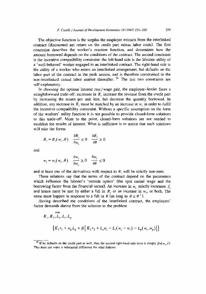
The objective function is the surplus the employer extracts from the interlinked contract (discounted net return on the credit part minus labor costs). The first constraint describes the worker 's reaction function, and determines how the amount borrowed depends on the conditions of the contract. The second constraint is the incentive compatibility constraint: the left-hand side is the lifetime utility of a 'well-behaved' worker engaged in an interlinked contract. The right-hand side is the utility of a worker who enters an interlinked arrangement, but defaults on the labor part of the contract in the peak season, and is therefore constrained to the non-interlinked casual labor market thereafter. 20 The last two constraints are self-explanatory.

In choosing the optimal interest ra te /wage pair, the employer-lender faces a straightforward trade-off: increases in R i increase the revenue from the credit part by increasing the return per unit lent, but decrease the quantity borrowed. In addition, any increase in R i must be matched by an increase in w i in order to fulfil the incentive compatibility constraint. Without a specific assumption on the form of the workers' utility function it is not possible to provide closed-form solutions to this trade-off. More to the point, closed-form solutions are not needed to establish the results of interest. What is sufficient is to notice that such solutions will take the forms

OR i ~R i - - < 0 > 0 aw c aO -

Ri=Ri(w~.,O)

and

W i = W i ( W c , 0 ) OW i OW i - - > _ 0 - - < 0 aw c a0 -

and at least one of the derivatives with respect to O, will be strictly non-zero. These relations say that the terms of the contract depend on the parameters

which influence the laborer's 'outside option' (the spot casual wage and the borrowing factor from the financial sector). An increase in wc strictly increases Jc and hence must be met by either a fall in R i or an increase in w i, or both. The same must happen in response to a fall in 0 (as long as 0 _< 0 * ).

Having described the conditions of the interlinked contract, the employers' factor demands derive from the solution to the problem

min

KI ,K2 ,La,Li,Lp

{K,r , + wpLp + fl[ K2r 2 + t a w c - Z i ( W c - W i ) - tp(Wc,Wp)]}

20 If he defaults on the credit part as well, then the second right-hand-side term is s imply flu(wc,~). This does not make a substantial difference for what follows.


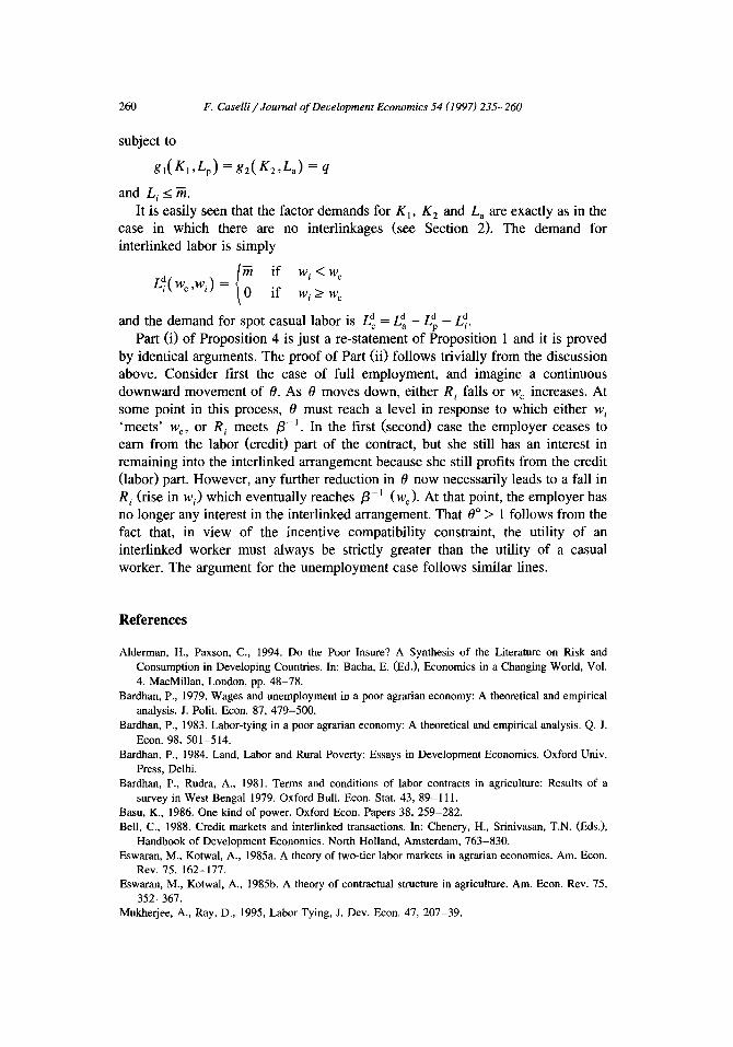
subject to

g l ( K i , L p ) = g e ( K z , L a ) = q

and L i < ~ . It is easily seen that the factor demands for K 1, K 2 and L a are exactly as in the

case in which there are no interlinkages (see Section 2). The demand for interlinked labor is simply

{O if w i < w c Ld( w c ' W i ) = if w i > w e

and the demand for spot casual labor is L~ = Lda -- L d - L d. Part (i) of Proposition 4 is just a re-statement of Proposition 1 and it is proved

by identical arguments. The proof of Part (ii) follows trivially from the discussion above. Consider first the case of full employment, and imagine a continuous downward movement of 0. As 0 moves down, either R; falls or w c increases. At some point in this process, 0 must reach a level in response to which either w i 'meets ' w e, or R i meets f l - l . In the first (second) case the employer ceases to earn from the labor (credit) part of the contract, but she still has an interest in remaining into the interlinked arrangement because she still profits from the credit (labor) part. However, any further reduction in 0 now necessarily leads to a fall in e i (rise in Wi) which eventually reaches /3 -1 (we). At that point, the employer has no longer any interest in the interlinked arrangement. That 0 ° > 1 follows from the fact that, in view of the incentive compatibility constraint, the utility of an interlinked worker must always be strictly greater than the utility of a casual worker. The argument for the unemployment case follows similar lines.

References

Alderman, H., Paxson, C., 1994. Do the Poor Insure? A Synthesis of the Literature on Risk and Consumption in Developing Countries. In: Bacha, E. (Ed.), Economics in a Changing World, Vol. 4. MacMillan, London, pp. 48-78.

Bardhan, P., 1979. Wages and unemployment in a poor agrarian economy: A theoretical and empirical analysis. J. Polit. Econ. 87, 479-500.

Bardhan, P., 1983. Labor-tying in a poor agrarian economy: A theoretical and empirical analysis. Q. J. Econ. 98, 501-514.

Bardhan, P., 1984. Land, Labor and Rural Poverty: Essays in Development Economics. Oxford Univ. Press, Delhi.

Bardhan, P., Rudra, A., 1981. Terms and conditions of labor contracts in agriculture: Results of a survey in West Bengal 1979. Oxford Bull. Econ. Stat. 43, 89-111.

Basu, K., 1986. One kind of power. Oxford Econ. Papers 38, 259-282. Bell, C., 1988. Credit markets and interlinked transactions. In: Chenery, H., Srinivasan, T.N. (Eds.),

Handbook of Development Economics. North Holland, Amsterdam, 763-830. Eswaran, M., Kotwal, A., 1985a. A theory of two-tier labor markets in agrarian economies. Am. Econ.

Rev. 75, 162-177. Eswaran, M., Kotwal, A., 1985b. A theory of contractual structure in agriculture. Am. Econ. Rev. 75,

352-367. Mukherjee, A., Ray, D., 1995, Labor Tying, J. Dev. Econ. 47, 207-39.

Documents

Rural labor and credit markets - LSE