Embed Size (px)
Citation preview
Runtime Compilation of Array-Oriented Python Programs
by
Alex Rubinsteyn
A dissertation submitted in partial ful�llment
of the requirements for the degree of
Doctor of Philosophy
Department of Computer Science
New York University
September 2014
Professor Dennis Shasha


Dedication
This thesis is dedicated to my parents and to the area code 60076.
iii
Acknowledgements
When I came to New York in 2007, I brought with me a Subaru Outback (mostly
full of books), a thinly acquired degree in Neuroscience, a rapidly shrinking bank ac-
count, and a nebulous plan to become a mathematician. When I wrote to a researcher
at MIT, seeking a position in his lab, I had to admit that: “my GPA is horrible, my rec-
ommendations grudgingly extracted from laughable sources.” To my earnest surprise,
he never replied. Undeterred and full of con�dence in the victory of my enthusiasm
over my historical inability to get anything done, I applied to Courant’s Masters pro-
gram in Mathematics and was promptly rejected. In a panic, I applied to Columbia’s
School of Continuing Education and was just as quickly turned away. I peppered them
with embarrassing pleas to reconsider, until one annoyed administrator replied that
“inconsistency and concern permeate each semester” of my transcript. Ouch.
That I still ended up having the privilege to pursue my curiosity feels like a miracle
and I owe a large debt of gratitude to many people. I would like to thank:
• My former project-mate Eric Hielscher, with whom I carved out many of the
ideas present in this thesis.
• My advisor, Dennis Shasha, who gave us guidance, support, discipline and choco-
late almonds.
• Professor Alan Siegel, who helped me get started on this grad school adventure,
taught me about algorithms, and got me a job which both paid the tuition for my
Masters and trained me in “butt-time” (meaning, I needed to learn how sit for
more than an hour).
• The job that Professor Siegel conjured for me was reading for Nektarios Paisios,
iv
who becamemy friend and collaborator. We worked together until he graduated,
and I think both bene�ted greatly from the arrangement.
• Professor Amir Pnueli, who was a great teacher and whose course in compilers
strongly in�uenced me.
• My �oor secretary, Leslie, who bravely shields us all from absurdities so we can
get work done. Without you, I probably would have dropped out by now.
• Ben, for being a great friend and making me leave my o�ce to eat dinner at
Quantum Leap.
• Geddes, for demolishing the walls we imagine between myth and reality. Stay
stubborn, reality doesn’t stand a chance.
• Most of all, I am grateful for a million things to my parents, Irene Zakon and
Arkady Rubinsteyn.
v
Abstract
The Python programming language has become a popular platform for data anal-
ysis and scienti�c computing. To mitigate the poor performance of Python’s standard
interpreter, numerically intensive computations are typically o�oaded to library func-
tions written in high-performance compiled languages such as Fortran or C. When
there is no e�cient library implementation available for a particular algorithm, the
programmer must accept suboptimal performance or switch to a low-level language to
implement the routine.
This thesis seeks to give Python programmers ameans to implement high-performance
algorithms in a high-level form. We present Parakeet, a runtime compiler for an array-
oriented subset of Python. Parakeet selectively augments the standard Python inter-
preter by compiling and executing functions explicitly marked for acceleration by the
programmer. Parakeet uses runtime type specialization to eliminate the performance-
defeating dynamicism of untyped Python code. Parakeet’s pervasive use of data paral-
lel operators as a means for implementing array operations enables high-level restruc-
turing optimization and compilation to parallel hardware such as multi-core CPUs
and graphics processors. We evaluate Parakeet on a collection of numerical bench-
marks and demonstrate its dramatic capacity for accelerating array-oriented Python
programs.
vi
Contents
Dedication . . . . . . . . . . . . . . . . . . . . . . . . . . . . . . . . . . . . . iii
Acknowledgements . . . . . . . . . . . . . . . . . . . . . . . . . . . . . . . . iv
Abstract . . . . . . . . . . . . . . . . . . . . . . . . . . . . . . . . . . . . . . . vi
List of Figures . . . . . . . . . . . . . . . . . . . . . . . . . . . . . . . . . . . xi
List of Tables . . . . . . . . . . . . . . . . . . . . . . . . . . . . . . . . . . . . xii
List of Code Listings . . . . . . . . . . . . . . . . . . . . . . . . . . . . . . . . xiii
List of Algorithms . . . . . . . . . . . . . . . . . . . . . . . . . . . . . . . . . xv
1 Introduction 1
2 Overview of Parakeet 7
2.1 Typed Intermediate Representation . . . . . . . . . . . . . . . . . . . . 9
2.2 Data Parallel Operators . . . . . . . . . . . . . . . . . . . . . . . . . . . 9
2.3 Compilation Process . . . . . . . . . . . . . . . . . . . . . . . . . . . . . 10
2.3.1 Type Specialization . . . . . . . . . . . . . . . . . . . . . . . . . 11
2.3.2 Optimization . . . . . . . . . . . . . . . . . . . . . . . . . . . . 12
2.4 Backends . . . . . . . . . . . . . . . . . . . . . . . . . . . . . . . . . . . 13
2.5 Limitations . . . . . . . . . . . . . . . . . . . . . . . . . . . . . . . . . . 14
2.6 Di�erences from Python . . . . . . . . . . . . . . . . . . . . . . . . . . 16
vii
2.7 Detailed Compilation Pipeline . . . . . . . . . . . . . . . . . . . . . . . 17
2.7.1 From Python into Parakeet . . . . . . . . . . . . . . . . . . . . 19
2.7.2 Untyped Representation . . . . . . . . . . . . . . . . . . . . . . 20
2.7.3 Type-specialized Representation . . . . . . . . . . . . . . . . . 21
2.7.4 Optimization . . . . . . . . . . . . . . . . . . . . . . . . . . . . 21
2.7.5 Generated C code . . . . . . . . . . . . . . . . . . . . . . . . . . 23
2.7.6 Generated x86 Assembly . . . . . . . . . . . . . . . . . . . . . . 23
2.7.7 Execution Times . . . . . . . . . . . . . . . . . . . . . . . . . . 23
3 History and Related Work 27
3.1 Array Programming . . . . . . . . . . . . . . . . . . . . . . . . . . . . . 29
3.2 Data Parallel Programming . . . . . . . . . . . . . . . . . . . . . . . . . 31
3.2.1 Collection-Oriented Languages . . . . . . . . . . . . . . . . . . 32
3.3 Related Projects . . . . . . . . . . . . . . . . . . . . . . . . . . . . . . . 33
4 Parakeet’s Intermediate Representation 35
4.1 Simple Expressions . . . . . . . . . . . . . . . . . . . . . . . . . . . . . 36
4.2 Statements and Control Flow . . . . . . . . . . . . . . . . . . . . . . . . 38
4.3 Array Properties . . . . . . . . . . . . . . . . . . . . . . . . . . . . . . . 40
4.4 Simple Array Operators . . . . . . . . . . . . . . . . . . . . . . . . . . . 40
4.5 Memory Allocation . . . . . . . . . . . . . . . . . . . . . . . . . . . . . 42
4.6 Higher Order Array Operators . . . . . . . . . . . . . . . . . . . . . . . 43
4.6.1 Mapping Operations . . . . . . . . . . . . . . . . . . . . . . . . 44
4.6.2 Reductions . . . . . . . . . . . . . . . . . . . . . . . . . . . . . 45
4.6.3 Scans . . . . . . . . . . . . . . . . . . . . . . . . . . . . . . . . . 45
4.7 Formal Syntax . . . . . . . . . . . . . . . . . . . . . . . . . . . . . . . . 46
viii
5 Type Inference and Specialization 48
5.1 Type System . . . . . . . . . . . . . . . . . . . . . . . . . . . . . . . . . 49
5.2 Type Specialization Algorithm . . . . . . . . . . . . . . . . . . . . . . . 50
5.2.1 Specialization Rules for Statements . . . . . . . . . . . . . . . . 51
5.2.2 Specialization Rules for Higher Array Operators . . . . . . . . 54
6 Optimizations 62
6.1 Standard Compiler Optimizations . . . . . . . . . . . . . . . . . . . . . 64
6.1.1 Simpli�cation . . . . . . . . . . . . . . . . . . . . . . . . . . . . 64
6.1.2 Dead Code Elimination . . . . . . . . . . . . . . . . . . . . . . . 64
6.1.3 Loop Invariant Code Motion . . . . . . . . . . . . . . . . . . . . 65
6.1.4 Scalar Replacement . . . . . . . . . . . . . . . . . . . . . . . . . 66
6.2 Fusion . . . . . . . . . . . . . . . . . . . . . . . . . . . . . . . . . . . . 66
6.2.1 Nested Fusion . . . . . . . . . . . . . . . . . . . . . . . . . . . . 68
6.2.2 Horizontal Fusion . . . . . . . . . . . . . . . . . . . . . . . . . . 68
6.3 Symbolic Execution and Shape Inference . . . . . . . . . . . . . . . . . 70
6.4 Value Specialization . . . . . . . . . . . . . . . . . . . . . . . . . . . . . 72
7 Evaluation 73
7.1 Growcut . . . . . . . . . . . . . . . . . . . . . . . . . . . . . . . . . . . 74
7.2 Matrix Multiplication . . . . . . . . . . . . . . . . . . . . . . . . . . . . 76
7.3 Rosenbrock Gradient . . . . . . . . . . . . . . . . . . . . . . . . . . . . 77
7.4 Image Convolution . . . . . . . . . . . . . . . . . . . . . . . . . . . . . 78
7.5 Univariate Regression . . . . . . . . . . . . . . . . . . . . . . . . . . . . 79
7.6 Tensor Rotation . . . . . . . . . . . . . . . . . . . . . . . . . . . . . . . 79
7.7 Harris Corner Detector . . . . . . . . . . . . . . . . . . . . . . . . . . . 81
ix

7.8 Julia Fractal . . . . . . . . . . . . . . . . . . . . . . . . . . . . . . . . . 82
7.9 Smoothed Particle Hydrodynamics . . . . . . . . . . . . . . . . . . . . 83
8 Conclusion 85
9 Bibliography 89
x
List of Figures
4.1 Parakeet’s Internal Syntax . . . . . . . . . . . . . . . . . . . . . . . . . 47
5.1 Types . . . . . . . . . . . . . . . . . . . . . . . . . . . . . . . . . . . . . 49
5.2 Scalar Subtype Hierarchy . . . . . . . . . . . . . . . . . . . . . . . . . . 50
5.3 Type Inference Helpers . . . . . . . . . . . . . . . . . . . . . . . . . . . 55
6.1 Fusion Rules . . . . . . . . . . . . . . . . . . . . . . . . . . . . . . . . . 69
6.2 Nested Fusion Rules . . . . . . . . . . . . . . . . . . . . . . . . . . . . . 71
6.3 Horizontal Fusion Rules . . . . . . . . . . . . . . . . . . . . . . . . . . . 71
xi
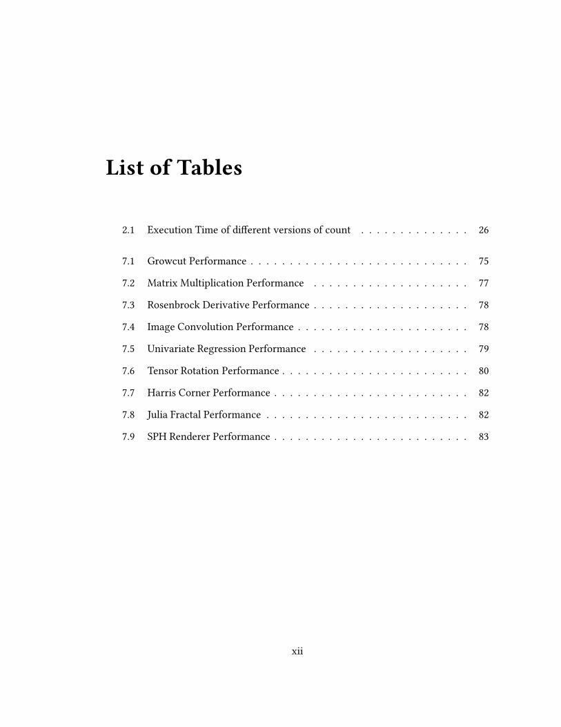
List of Tables
2.1 Execution Time of di�erent versions of count . . . . . . . . . . . . . . 26
7.1 Growcut Performance . . . . . . . . . . . . . . . . . . . . . . . . . . . . 75
7.2 Matrix Multiplication Performance . . . . . . . . . . . . . . . . . . . . 77
7.3 Rosenbrock Derivative Performance . . . . . . . . . . . . . . . . . . . . 78
7.4 Image Convolution Performance . . . . . . . . . . . . . . . . . . . . . . 78
7.5 Univariate Regression Performance . . . . . . . . . . . . . . . . . . . . 79
7.6 Tensor Rotation Performance . . . . . . . . . . . . . . . . . . . . . . . . 80
7.7 Harris Corner Performance . . . . . . . . . . . . . . . . . . . . . . . . . 82
7.8 Julia Fractal Performance . . . . . . . . . . . . . . . . . . . . . . . . . . 82
7.9 SPH Renderer Performance . . . . . . . . . . . . . . . . . . . . . . . . . 83
xii
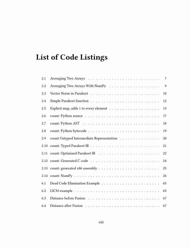
List of Code Listings
2.1 Averaging Two Arrays . . . . . . . . . . . . . . . . . . . . . . . . . . . 7
2.2 Averaging Two Arrays With NumPy . . . . . . . . . . . . . . . . . . . 9
2.3 Vector Norm in Parakeet . . . . . . . . . . . . . . . . . . . . . . . . . . 10
2.4 Simple Parakeet function . . . . . . . . . . . . . . . . . . . . . . . . . . 12
2.5 Explicit map, adds 1 to every element . . . . . . . . . . . . . . . . . . . 13
2.6 count: Python source . . . . . . . . . . . . . . . . . . . . . . . . . . . . 17
2.7 count: Python AST . . . . . . . . . . . . . . . . . . . . . . . . . . . . . 18
2.8 count: Python bytecode . . . . . . . . . . . . . . . . . . . . . . . . . . . 19
2.9 count Untyped Intermediate Representation . . . . . . . . . . . . . . . 20
2.10 count: Typed Parakeet IR . . . . . . . . . . . . . . . . . . . . . . . . . . 21
2.11 count: Optimized Parakeet IR . . . . . . . . . . . . . . . . . . . . . . . 22
2.12 count: Generated C code . . . . . . . . . . . . . . . . . . . . . . . . . . 24
2.13 count: generated x86 assembly . . . . . . . . . . . . . . . . . . . . . . . 25
2.14 count: NumPy . . . . . . . . . . . . . . . . . . . . . . . . . . . . . . . . 26
6.1 Dead Code Elimination Example . . . . . . . . . . . . . . . . . . . . . . 65
6.2 LICM example . . . . . . . . . . . . . . . . . . . . . . . . . . . . . . . . 65
6.3 Distance before Fusion . . . . . . . . . . . . . . . . . . . . . . . . . . . 67
6.4 Distance after Fusion . . . . . . . . . . . . . . . . . . . . . . . . . . . . 67
xiii
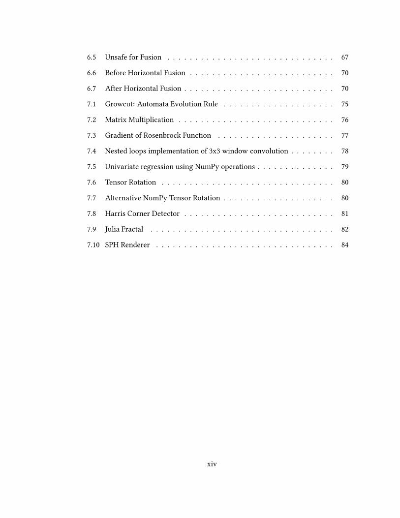
6.5 Unsafe for Fusion . . . . . . . . . . . . . . . . . . . . . . . . . . . . . . 67
6.6 Before Horizontal Fusion . . . . . . . . . . . . . . . . . . . . . . . . . . 70
6.7 After Horizontal Fusion . . . . . . . . . . . . . . . . . . . . . . . . . . . 70
7.1 Growcut: Automata Evolution Rule . . . . . . . . . . . . . . . . . . . . 75
7.2 Matrix Multiplication . . . . . . . . . . . . . . . . . . . . . . . . . . . . 76
7.3 Gradient of Rosenbrock Function . . . . . . . . . . . . . . . . . . . . . 77
7.4 Nested loops implementation of 3x3 window convolution . . . . . . . . 78
7.5 Univariate regression using NumPy operations . . . . . . . . . . . . . . 79
7.6 Tensor Rotation . . . . . . . . . . . . . . . . . . . . . . . . . . . . . . . 80
7.7 Alternative NumPy Tensor Rotation . . . . . . . . . . . . . . . . . . . . 80
7.8 Harris Corner Detector . . . . . . . . . . . . . . . . . . . . . . . . . . . 81
7.9 Julia Fractal . . . . . . . . . . . . . . . . . . . . . . . . . . . . . . . . . 82
7.10 SPH Renderer . . . . . . . . . . . . . . . . . . . . . . . . . . . . . . . . 84
xiv
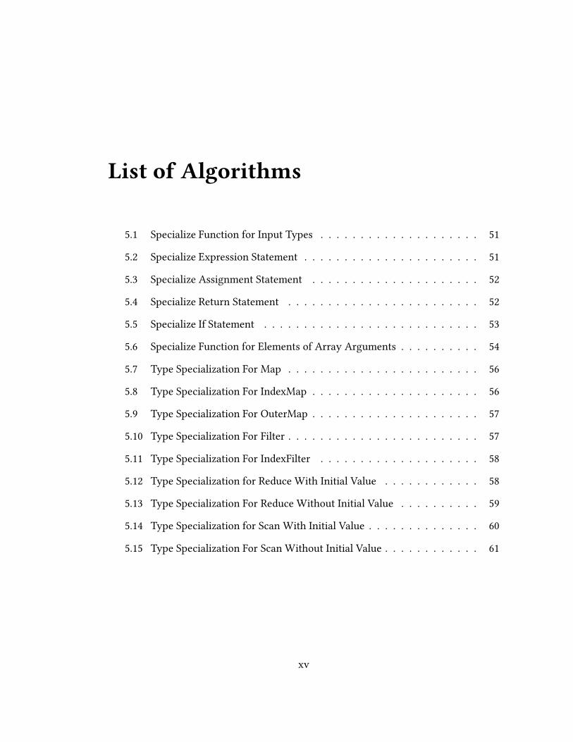
List of Algorithms
5.1 Specialize Function for Input Types . . . . . . . . . . . . . . . . . . . . 51
5.2 Specialize Expression Statement . . . . . . . . . . . . . . . . . . . . . . 51
5.3 Specialize Assignment Statement . . . . . . . . . . . . . . . . . . . . . 52
5.4 Specialize Return Statement . . . . . . . . . . . . . . . . . . . . . . . . 52
5.5 Specialize If Statement . . . . . . . . . . . . . . . . . . . . . . . . . . . 53
5.6 Specialize Function for Elements of Array Arguments . . . . . . . . . . 54
5.7 Type Specialization For Map . . . . . . . . . . . . . . . . . . . . . . . . 56
5.8 Type Specialization For IndexMap . . . . . . . . . . . . . . . . . . . . . 56
5.9 Type Specialization For OuterMap . . . . . . . . . . . . . . . . . . . . . 57
5.10 Type Specialization For Filter . . . . . . . . . . . . . . . . . . . . . . . . 57
5.11 Type Specialization For IndexFilter . . . . . . . . . . . . . . . . . . . . 58
5.12 Type Specialization for Reduce With Initial Value . . . . . . . . . . . . 58
5.13 Type Specialization For Reduce Without Initial Value . . . . . . . . . . 59
5.14 Type Specialization for Scan With Initial Value . . . . . . . . . . . . . . 60
5.15 Type Specialization For Scan Without Initial Value . . . . . . . . . . . . 61
xv
Chapter 1
Introduction
I’m not a programmer, I’m a statistician. I sit in a room with pencil and paper
coming up with new models and working out the mathematics behind them. I
only program because no one else is going to code my models for me.
— Comment on reddit.com
It is a hallmark of our data saturated age thatmany self identi�ed non-programmers
�nd themselves trying to tell a computer what to do. Scientists need to distill the nu-
merical deluge spewing from their experiments, the quants of Wall Street want to pre-
dict the movement of chaotic markets, and seemingly everyone wants to analyze your
data on the internet. Similarly, many professional programmers (who don’t identify as
scientists or statisticians) are wading into the numerical fray to �lter, transform and
summarize an increasingly quanti�ed world.
Against this backdrop of non-programmers programming and non-numericists nu-
mericizing, the Python programming language [VRDJ95] has emerged as a popular
environment for number crunching and data analysis. This may come as a surprise
since, unlike Mathematica [Wol99], Matlab [MAT10] or R [IG96], Python was not
originally conceived of as a “mathematical”, “numerical” or “statistical” programming
1
language. However, by virtue of Python’s semantic �exibility and easy interoperabil-
ity with lower-level languages, Python has grown an extremely rich ecosystem of
scienti�c libraries. These include NumPy [Oli06] and Pandas [McK11], which pro-
vide expressive numerical data structures, SciPy [JOP01], a generous repository of
mathematical functions, and matplotlib [Hun07], a �exible plotting package. The ver-
satility of these tools, along with vibrancy of the communities which develop and
use them, has led to Python becoming the lingua franca in several scienti�c disci-
plines [MGS07, PGH11, Gre07, Blo03].
But isn’t Python slow? In fact, yes, the standard language implementation (a byte-
code interpreter calledCPython) can be orders ofmagnitude slower than statically com-
piled lower-level languages such as C and Fortran. If your goal is to quickly perform
some repetitive arithmetic on a large collection of numbers, then ideally those num-
bers would be stored contiguously in memory, loaded into registers in small groups,
and acted upon by a compact set of native machine instructions. The Python inter-
preter, on the other hand, represents values using bulky heap allocated objects and
even simple operations, like multiplying two numbers, are implemented using exten-
sive indirection.
If the Python interpreter’s ine�ciencies could not be somehow eliminated then
would-be users of numerical Python tools would balk at sub-standard performance. In
fact, a recent survey [PJR+11] of computational practices among scientists noted that:
Nothing evoked stronger reactions during the interviews than questions
regarding the impact of faster computation...Faster computation enables ac-
curate scienti�cmodelingwithin time scales previously thought unattainable.
The key to satisfying these performance-hungry scientists and getting good numer-
ical performance from Python is to o�-load computationally intensive tasks to lower-
2
level library code. If an algorithm spends most of its time performing some common
operation through an e�cient library – matrix multiplication using ATLAS [WPD01],
or Fourier transforms through FFTW [FJ05] – then there should be no signi�cant
performance di�erence between a Python implementation and an equivalent program
using the same libraries from a more e�cient language.
The NumPy array library [Oli06] plays an important role in enabling the use of
e�cient algorithmic implementations from within Python by providing a high level
Pythonic interface around unboxed arrays. These arrays can be passed easily into pre-
compiled C or Fortran code. The NumPy array is the de facto numerical container for
Python programs, on top of which other data structures are typically constructed.
NumPy’s mode of library-centric development provides acceptable performance as
long as the algorithm you are implementing can be expressed primarily in terms of ex-
isting compiled primitives. However, a developer may need to implement a novel “in-
ner loop”, for which no precompiled equivalent exists. In this case, they are faced with
two frustrating choices: either implement their desired computation in pure Python
(and thus su�er a severe performance penalty) or write in some lower-level language,
and face a dramatic loss of productivity [Pre03]. For example, the developers of the
widely used scikit-learn [PVG+11] machine learning library spent about half a year of
development time reviewing and integrating a statically compiled implementation of
decision tree ensembles. A pure Python version would have been dramatically shorter
and simpler, but had little chance of attaining su�ciently fast performance.
To make things worse, merely moving a bottleneck into a lower-level language
is unlikely to fully utilize a computer’s available computational resources. A mod-
ern desktop computer will typically have somewhere between 2-8 cores and a graph-
ics processor (GPU) capable of general-purpose computation. GPUs are highly par-
3

allel “many-core” architectures which, depending on the task, can be 10x-100x faster
than multi-core CPU algorithms [OHL+08, Kin12, KY13]. Several �elds of research,
such as deep neural networks [KSH12], have become entirely reliant on the computa-
tional power of GPUs to perform tasks which would be infeasibly slow on the CPU.
Unfortunately taking advantage of all this parallel hardware is not easy. Splitting a
computation across multiple cores necessitates either manually using a threading li-
brary [NBF96] or a parallel API such as OpenMP [DM98]. GPU acceleration necessi-
tates evenmore programmer e�ort, requiring intimate knowledge of the graphics hard-
ware and the use of a specialized language such as CUDA [Nvi11] or OpenCL [SGS10].
What may have began as an elegant prototype in Python runs the risk of devolving
into a complex and error-prone exercise in parallel programming.
In between the unsatisfactory performance/productivity pro�les of purely high
level and purely low level implementations runs the middle road of runtime compi-
lation. Common sources of ine�ciency in a high level language’s implementation –
such as dynamic dispatch and tagged heap-allocated data representations – can be by-
passed if native code gets generated at runtime, when su�cient information is present
for specialized compilation.
It may even be possible to use high level algorithmic descriptions, extracted from a
language such as Python, to generate code which is faster than an implementation in C
or Fortran. There are several factors which could contribute to a signi�cant speed-up
over manually crafted low level code:
• Pre-compiled performance primitives must be separately compiled and thus can-
not perform optimizations which arise when these routines are used together.
Thus, the composition of multiple such functions may incur wasteful overhead.
For example, a quantity may be computed repeatedly, once per function being
4

called or large temporary values may be created where a more holistic view of
the code could have avoided any extra allocation or data traversal. On the other
hand, operations in a high level description of a numerical algorithm can be fused
and rearranged to ultimately attain a faster implementation.
• Implementing a performance-sensitive portion of an algorithm in C or Fortran
does not, by itself, do anything to harness the woefully underutilized parallel
hardware found in most modern machines. If, for example, a programmer wants
to move some computation to their GPU, they must learn an unfamiliar and
tricky programming model such as OpenCL [SGS10] or CUDA [Nvi11]. High
level algorithmic descriptions, on the other hand, are rife with �exible evaluation
orders and opportunities for parallel execution. If there is any hope of making
general-purpose GPU programming an easy and accessible activity, it will likely
come from the automatic translation of high level programs to the GPU.
• Since the actual values of the computational inputs are available at runtime, it is
possible to partially evaluate the programmer’s code on portions of those values
which may signi�cantly impact performance. For example, many routines in the
NumPy array library must either explicitly provide specializations for particular
data layouts or fall back upon slower layout-agnostic implementations. Runtime
value specialization, enabled in the context of a runtime compiler, allows for the
possibility of generating conservative layout-agnostic code and then specializing
it for the “array strides” of a particular input.
This thesis seeks to give Python programmers ameans to implement high-performance
parallel algorithms in a high level form. We present Parakeet [RHWS12], a runtime
compiler for an array-oriented subset of Python. Parakeet aims to allow compact high
5
level speci�cation of numerically intensive algorithms which attain performance com-
parable to more verbose implementations in lower-level languages. Toward this per-
formance goal we employ type specialization and the permissive semantics of data par-
allel operators which enable sophisticated optimizations and parallel execution across
multiple cores and on the GPU.
The major contributions of this thesis are:
1. A demonstration that runtime-compiled implicitly parallel numerical program-
ming can signi�cantly outperform precompiledNumPy library functions and run
in parallel across multiple cores and on the GPU.
2. A type inference algorithm which propagates input types throughout a function
to derive specialized code.
3. A rich system of high order data parallel operators, such as the familiar Map,
Reduce, Scan but also more esoteric or previously unseen operators such as In-
dexReduce, FilterReduce, andOuterMap. Parakeet uni�es the closely related
paradigms of array languages and data-parallel programming by desugaring high
level array constructs into explicit uses of data parallel operations.
The combined e�ect of Parakeet’s typed representation, high level optimizations
and use of the GPU or multi-core parallelism is a signi�cant and consistent acceleration
of numerical Python programs. For those programs which consist primarily of calls to
NumPy library functions, Parakeet may speed them up by an order of magnitude. For
programs which perform most of their computations within the Python interpreter,
Parakeet’s speedup can reach into the tens of thousands.
6
Chapter 2
Overview of Parakeet
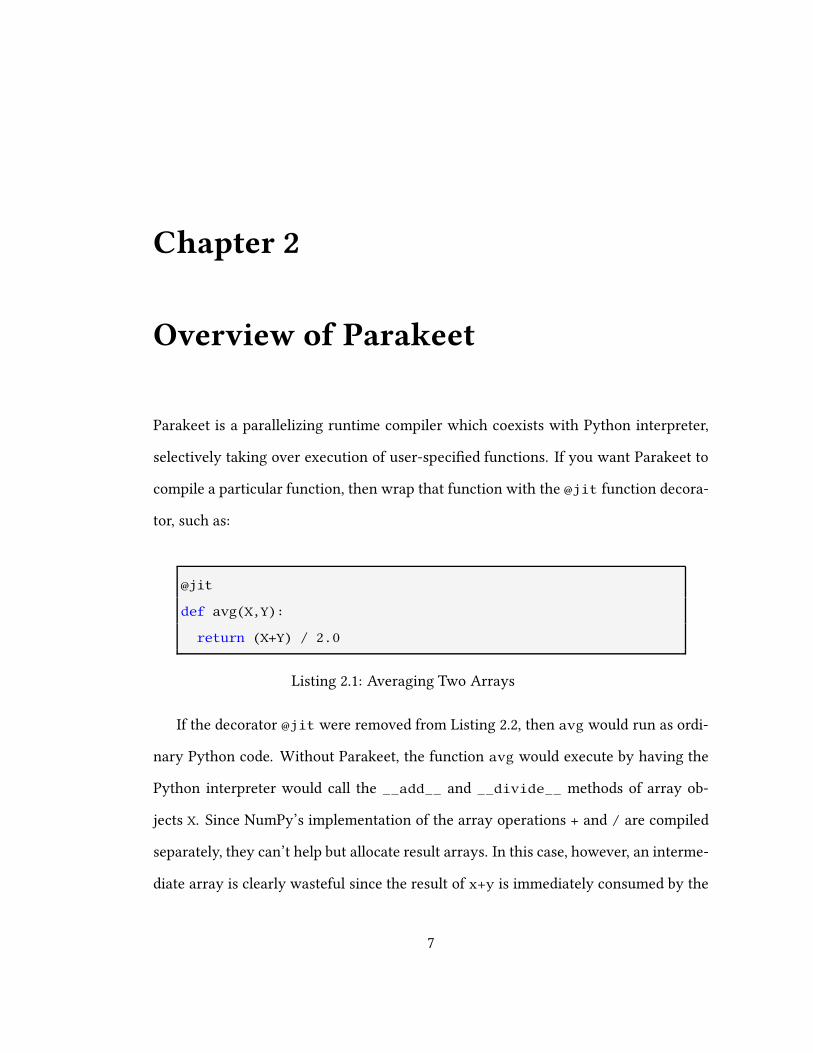
Parakeet is a parallelizing runtime compiler which coexists with Python interpreter,
selectively taking over execution of user-speci�ed functions. If you want Parakeet to
compile a particular function, then wrap that function with the @jit function decora-
tor, such as:
@jit
def avg(X,Y):
return (X+Y) / 2.0
Listing 2.1: Averaging Two Arrays
If the decorator @jit were removed from Listing 2.2, then avg would run as ordi-
nary Python code. Without Parakeet, the function avg would execute by having the
Python interpreter would call the __add__ and __divide__ methods of array ob-
jects X. Since NumPy’s implementation of the array operations + and / are compiled
separately, they can’t help but allocate result arrays. In this case, however, an interme-
diate array is clearly wasteful since the result of x+y is immediately consumed by the
7
division.
On the other hand, Parakeet specializes avg for any distinct input type, optimizes
its body into a single combined array operation (avoiding unnecessary allocation) and
executes it as parallel native code.
The @jit decorator cannot be used on any arbitrary Python function since Para-
keet is not a general-purpose compiler for all of Python. The job of the @jit decorator
is to intercept calls into a wrapped function and then to initiate the following chain of
events:
1. Translate the function into an untyped representation, from which we’ll later
derive multiple type specializations.
2. Specialize the untyped function for the current argument types, creating a typed
version of the function.
3. Aggressively optimize the typed code, leveraging the high-level intermediate
representation to perform optimizations which would be more di�cult in C or
Fortran.
4. Lower the optimized code into a parallel low-level implementation using either
OpenMP (for multi-core execution) or CUDA (for the GPU).
Parakeet only supports a handful of Python’s data types (numbers, tuples, slices,
and NumPy arrays). To manipulate these values, Parakeet lets the programmer use
any of the usual math and logic operators, along with a subset of built-in and NumPy
library functions. If your performance bottleneck doesn’t �t neatly into Parakeet’s
restrictive universe then you might bene�t from a faster Python implementation such
as PyPy [RP06], or alternatively you could outsource some of your functionality to
native code via Cython [BBC+11] or an extension module written in C or Fortran.
8

2.1 Typed Intermediate Representation
Parakeet uses a typed intermediate representation: unlike Python, every variable is
annotated with a type annotation. Furthermore, operations such as adding are sig-
ni�cantly more restricted (or perhaps, “static”) than their equivalents in Python. For
example, unlike Python, the addition operator + does not signify dynamic dispatch on
the __add__ method. Rather, in Parakeet’s intermediate representation, each occur-
rence of + can only act on scalar values of a certain type. Arithmetic operators between
array values must expressed more explicitly using data parallel operators such asMap.
For example, if the function in Listing 2.2 were passed two �oat vectors, then Parakeet’s
typed intermediate representation of this would look like:
def avg(X :: array1(float32), Y :: array1(float32)):
temp :: float32 = Map(lambda xi, yi: xi + yi, X, Y)
return Map(lambda xi: xi / 2.0, temp)
Listing 2.2: Averaging Two Arrays With NumPy
2.2 Data Parallel Operators
Parallelism in Parakeet is achieved through the implicit or explicit use of data parallel
operators. Some examples of these operators are listed below:
• Map(f, X1, ..., Xn, axis=None)
Apply the function f to each element of the array arguments. By default f is
passed each scalar element of the array arguments. The axis keyword can be
used to specify a di�erent iteration pattern (such as applying f to all columns).
• Reduce(combine, X1, ...,Xn, axis=None, init=None)
9

Combine all the elements of the array arguments using the binary commutative
function combine. The init keyword is an optional initial value for the reduction.
Examples of reductions are the NumPy functions sum and product.
• Scan(combine, X1, ...,Xn, axis=None, init=None)
Combine all the elements of the array arguments and return an array containing
all cumulative intermediate values of the combination. Examples of scans are the
NumPy functions cumsum and cumprod.
For each occurrence of a data parallel operator in a program, Parakeet may choose
to synthesize parallel code which implements that operator combined with its function
argument. It is not always necessary, however, to explicitly use one of these operators
in order to achieve parallelization. Parakeet implements NumPy’s array broadcasting
semantics by implicitly inserting calls toMap into a user’s code. Furthermore, NumPy
library functions are reimplemented in Parakeet using the above data parallel operators
and thus expose opportunities for parallelism.
2.3 Compilation Process
We will refer to the following code example to help illustrate the process by which
Parakeet transforms and executes code.
@jit
def norm(x):
return np.sqrt(sum(x*x))
Listing 2.3: Vector Norm in Parakeet
10
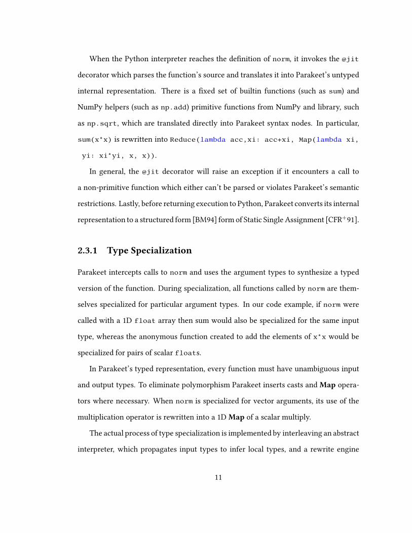
When the Python interpreter reaches the de�nition of norm, it invokes the @jit
decorator which parses the function’s source and translates it into Parakeet’s untyped
internal representation. There is a �xed set of builtin functions (such as sum) and
NumPy helpers (such as np.add) primitive functions from NumPy and library, such
as np.sqrt, which are translated directly into Parakeet syntax nodes. In particular,
sum(x*x) is rewritten into Reduce(lambda acc,xi: acc+xi, Map(lambda xi,
yi: xi*yi, x, x)).
In general, the @jit decorator will raise an exception if it encounters a call to
a non-primitive function which either can’t be parsed or violates Parakeet’s semantic
restrictions. Lastly, before returning execution to Python, Parakeet converts its internal
representation to a structured form [BM94] form of Static Single Assignment [CFR+91].
2.3.1 Type Specialization
Parakeet intercepts calls to norm and uses the argument types to synthesize a typed
version of the function. During specialization, all functions called by norm are them-
selves specialized for particular argument types. In our code example, if norm were
called with a 1D float array then sum would also be specialized for the same input
type, whereas the anonymous function created to add the elements of x*x would be
specialized for pairs of scalar floats.
In Parakeet’s typed representation, every function must have unambiguous input
and output types. To eliminate polymorphism Parakeet inserts casts and Map opera-
tors where necessary. When norm is specialized for vector arguments, its use of the
multiplication operator is rewritten into a 1D Map of a scalar multiply.
The actual process of type specialization is implemented by interleaving an abstract
interpreter, which propagates input types to infer local types, and a rewrite engine
11

which inserts coercions where necessary.
2.3.2 Optimization
In addition to standard compiler optimizations (such as constant folding, function inlin-
ing, and common sub-expression elimination), we employ fusion rules [AS79, JTH01,
KM93] to combine array operators. Fusion enables us to increase the computational
density of generated code and to avoid the creation of unnecessary array temporaries.
Using Parakeet can be as simple as calling a Parakeet library function from within
existing Python code. For example, the �rst call to parakeet.mean(matrix) will
compile a small program to e�ciently average the rows of amatrix in parallel. Repeated
calls will not incur further compilation costs. If a Python function is wrapped with the
@parakeet.jit decorator, then its body will be parsed by Parakeet and prepared for
later compilation. When such a function is �nally called, its untyped syntax will be
specialized for the types of the given arguments and then compiled and executed. For
example, consider the simple function shown in Figure 2.4.
@parakeet.jit
def add1(x):
return x+1
Listing 2.4: Simple Parakeet function
If add1 is called with an integer argument, then it will be compiled to return an
integer result. If, however, add1 is later called with a �oating point input then a new
native implementation will be compiled that computes a �oating point result.
This example does not make use of any data parallel operators. In fact, it is possible
to generate code with Parakeet using only its capacity to e�ciently compile loops and
scalar operations. However, even greater performance gains can be achieved through
12
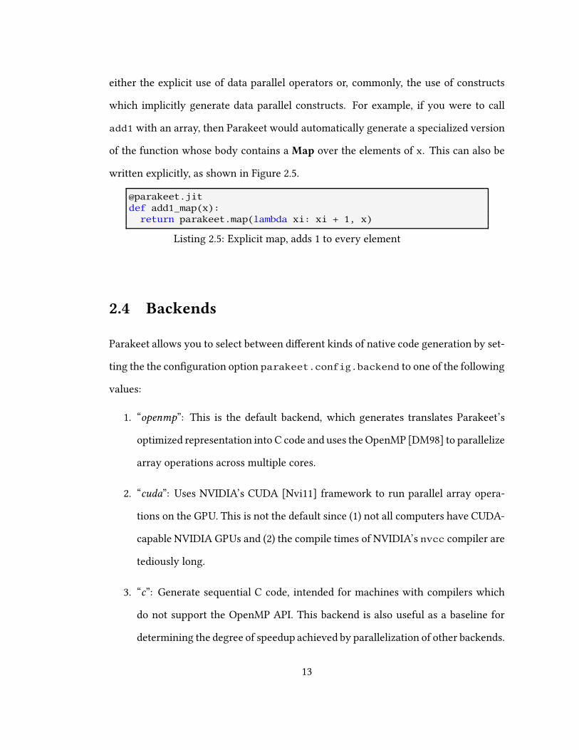
either the explicit use of data parallel operators or, commonly, the use of constructs
which implicitly generate data parallel constructs. For example, if you were to call
add1 with an array, then Parakeet would automatically generate a specialized version
of the function whose body contains a Map over the elements of x. This can also be
written explicitly, as shown in Figure 2.5.
@parakeet.jitdef add1_map(x):
return parakeet.map(lambda xi: xi + 1, x)
Listing 2.5: Explicit map, adds 1 to every element
2.4 Backends
Parakeet allows you to select between di�erent kinds of native code generation by set-
ting the the con�guration option parakeet.config.backend to one of the following
values:
1. “openmp”: This is the default backend, which generates translates Parakeet’s
optimized representation into C code and uses the OpenMP [DM98] to parallelize
array operations across multiple cores.
2. “cuda”: Uses NVIDIA’s CUDA [Nvi11] framework to run parallel array opera-
tions on the GPU. This is not the default since (1) not all computers have CUDA-
capable NVIDIA GPUs and (2) the compile times of NVIDIA’s nvcc compiler are
tediously long.
3. “c”: Generate sequential C code, intended for machines with compilers which
do not support the OpenMP API. This backend is also useful as a baseline for
determining the degree of speedup achieved by parallelization of other backends.
13
4. “interp”: Pure Python interpreter for Parakeet’s intermediate representation, used
primarily for internal debugging purposes, in general runs signi�cantly slower
than Python.
Rather than modifying a global con�guration option, it is also possible to pass the
name of the desired backend when calling into a Parakeet function with the keyword
argument _backend.
2.5 Limitations
Parakeet is a runtime compiler for numerically intensive algorithms written in Python.
In comparison with arbitrary Python code, Parakeet programs are very constrained.
This is because Parakeet trades dynamicism and complexity for greater latitude in pro-
gram transformation and ultimately the ability to generate e�cient low-level code (we
still have high-level constructs, they’re just well behaved). The features which Para-
keet does support are chosen to facilitate array-oriented numerical algorithms such as
those found in machine learning, �nancial computing, and scienti�c simulation. The
sections of code that Parakeet accelerates must obey the following constraints:
• The only data types which can be used within code compiled by Parakeet are
tuples, scalars, slices, NumPy arrays, and the None object. Other data types, such
as sets, dictionaries, generators, and user-de�ned objects are not supported.
• Due to Parakeet’s use of a simpli�ed program representation, only “structured" [BM94]
control �ow is allowed. This precludes the use of exceptions, as well as the break
and continue statements.
14
• Since Parakeet must have access to a function’s source, any compiled C exten-
sions (or functions which call C extensions) cannot be used within Parakeet.
• Parakeet treats aggregate structures such as slices and arrays as immutable and
the programmer cannot modify the values of their �elds. The data contained
within an array, however, can be modi�ed. Similarly, the value of a local vari-
able can be updated. So, though Parakeet does restrict where mutability can hap-
pen, Parakeet does not require the programmer to adhere to a purely functional
programming style (unlike Copperhead [CGK11]).
• To compile Python into native code we must assign types to each expression. We
are still able to retain some of Python’s polymorphism by specializing di�erent
typed versions of a function for each distinct set of argument types. However,
expressions whose types depend on dynamic values are disallowed (e.g. 42 if
bool_val else (1,2,3)).
• A Parakeet function cannot call any other function which violates these restric-
tions or one which is not implemented in Python. These restrictions recursively
apply down the call chain, so that the use of an invalid construct by a function
also taints any other functions which call it.
• To enable the use of NumPy library functions Parakeet must provide equiva-
lent functions written in Python. However, some NumPy functions are not yet
implemented and others use language constructs which make their inclusion in
Parakeet unlikely to ever occur. For a full listing of which NumPy functions are
supported, the programmer can look in the parakeet.mapping module.
15
These restrictions would be onerous if applied to an entire program but Parakeet
is only intended to accelerate the computational core of an algorithm. All other code
is executed as usual by the Python interpreter.
2.6 Di�erences from Python
In addition to restrictions on what sort of source code will even be accepted by Para-
keet’s frontend, there are also some semantic di�erences which may result in Parakeet
computing a di�erent value from Python.
• Since Parakeet does not implement Python lists, any list literals are treated as
arrays. Similarly, list comprehensions are reinterpreted as (parallel) array com-
prehensions.
• Some expressions which seem to have conditionally dependent types will suc-
cessfully be translated into Parakeet, but only by casting both values of a con-
ditional into a single unifying type. For example, the Python expression 3 if
bool_val else 2.0will selectively return either an integer or a �oating point
value but Parakeet will upcast the 3 into a 3.0.
• Parakeet’s reimplementation of NumPy library functions does not currently sup-
port non-essential parameters such as output.
• Parakeet’s parallel backends (OpenMP and CUDA) may change the order of a
�oating-point reductions (such as summing the elements of an array), resulting
in small di�erences relative to Python due to the slight non-commutativity of
�oating point math.
16

• Parakeet implements NumPy’s array broadcasting using a translation scheme
dependent on the types of arguments. For example, adding a matrix and a vector
together will be correctly translated into a Map which adds the vector to each
column of the matrix. The full semantics of broadcasting, however, also allows
for array elements to be replicated due to the values of an array’s shape, which
are not evident in the type signature. For example, adding a 200x1 matrix with a
1x300 matrix in NumPy will yield a 200x300 result. Parakeet, however, does not
implement this correctly and will give an erroneous result.
2.7 Detailed Compilation Pipeline
In this section, we follow a simple function on its journey through the Parakeet JIT
compiler to elucidate how Parakeet translates high level code into high performance,
native versions. The function we will compile is the count function shown in Figure
2.6, which sums up the number of elements in an array less than a given threshold.
We use a loop in this example rather than an adverb for now, as our focus is on the
Parakeet compilation pipeline.
@parakeet.jitdef count(values, thresh):
n = 0for elt in values:
n += elt < threshreturn n
Listing 2.6: count: Python source
This function is simple, but it’s not an entirely contrived computation. For example,
it forms the core of a decision tree learning algorithm. Before breaking down how
Parakeet compiles count, let’s �rst look at how the original gets executed within the
17

standard CPython interpreter.
The �rst thing that happens to a function on its way to being executed is parsing.
The source of count gets read as a string of characters, tokenized, and then turned
into a structured syntax tree as shown in Figure 2.7.
FunctionDef(name=’count’,args=arguments(args=[Name(id=’values’), Name(id=’thresh’)],
vararg=None, kwarg=None, defaults=[]),body=[
Assign(targets=[Name(id=’n’)], value=Num(n=0)),For(target=Name(id=’elt’), iter=Name(id=’values’), body=[
AugAssign(target=Name(id=’n’), op=Add(),value=Compare(left=Name(id=’elt’), ops=[Lt()],
comparators=[Name(id=’thresh’)]))]),Return(value=Name(id=’n’, ctx=Load()))])
Listing 2.7: count: Python AST
A naive interpreter would then execute the syntax tree directly. Python achieves a
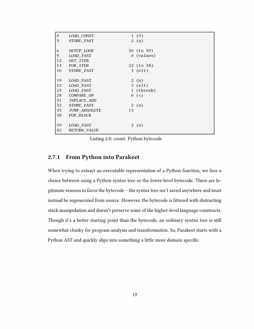
minor performance boost by instead compiling to a more compact bytecode, as shown
in Figure 2.8.
The ine�ciency of tree-walking interpreters (which evaluate syntax trees) com-
pared with bytecode execution is one of the reasons that Ruby has generally been
slower than Python. Though an improvement over a naive interpreter, trying to exe-
cute this bytecode directly still results in terrible performance. If you inspect the be-
havior of the above instructions, you’ll discover that they involve repetitive un-boxing
and re-boxing of numeric values in and out of their PyObject wrappers, wasteful stack
manipulation, and a lot of other very wasteful computations. If we’re going to sig-
ni�cantly speed up the numerical performance of Python code, it’s going to have run
somewhere other than the CPython bytecode interpreter.
18
0 LOAD_CONST 1 (0)3 STORE_FAST 2 (n)
6 SETUP_LOOP 30 (to 39)9 LOAD_FAST 0 (values)12 GET_ITER13 FOR_ITER 22 (to 38)16 STORE_FAST 3 (elt)
19 LOAD_FAST 2 (n)22 LOAD_FAST 3 (elt)25 LOAD_FAST 1 (thresh)28 COMPARE_OP 0 (<)31 INPLACE_ADD32 STORE_FAST 2 (n)35 JUMP_ABSOLUTE 1338 POP_BLOCK
39 LOAD_FAST 2 (n)42 RETURN_VALUE
Listing 2.8: count: Python bytecode
2.7.1 From Python into Parakeet
When trying to extract an executable representation of a Python function, we face a
choice between using a Python syntax tree or the lower-level bytecode. There are le-
gitimate reasons to favor the bytecode – the syntax tree isn’t saved anywhere andmust
instead be regenerated from source. However, the bytecode is littered with distracting
stack manipulation and doesn’t preserve some of the higher-level language constructs.
Though it’s a better starting point than the bytecode, an ordinary syntax tree is still
somewhat clunky for program analysis and transformation. So, Parakeet starts with a
Python AST and quickly slips into something a little more domain speci�c.
19
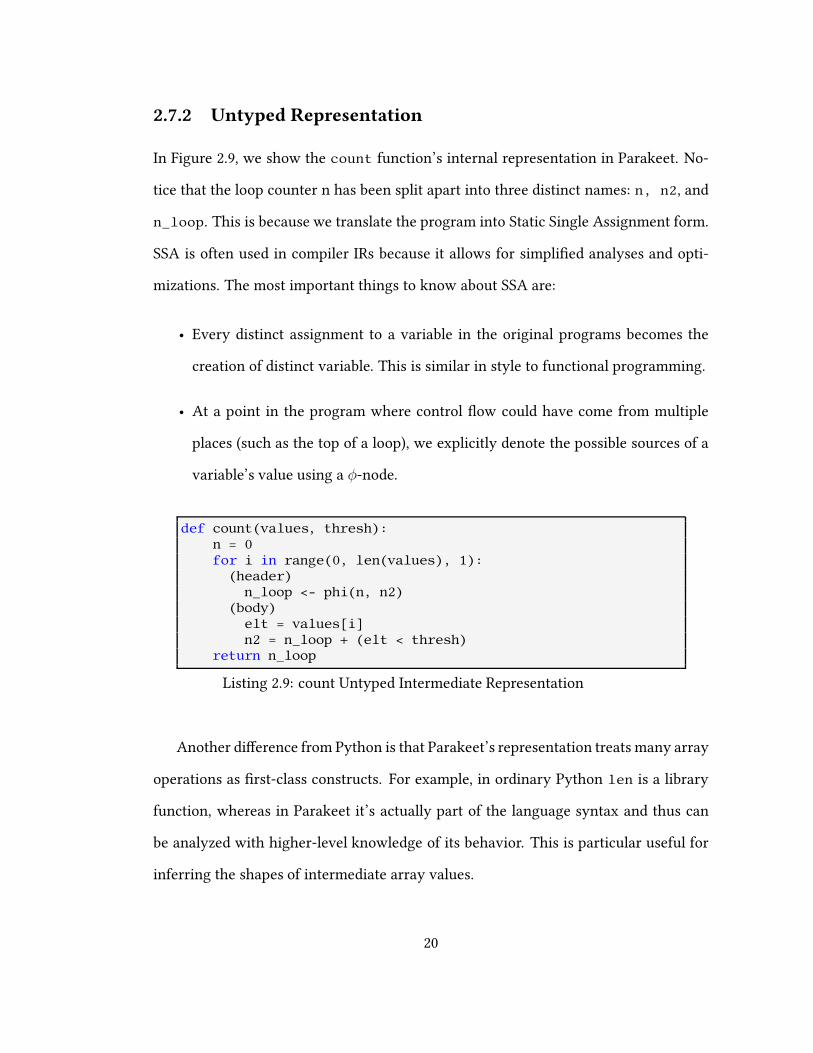
2.7.2 Untyped Representation
In Figure 2.9, we show the count function’s internal representation in Parakeet. No-
tice that the loop counter n has been split apart into three distinct names: n, n2, and
n_loop. This is because we translate the program into Static Single Assignment form.
SSA is often used in compiler IRs because it allows for simpli�ed analyses and opti-
mizations. The most important things to know about SSA are:
• Every distinct assignment to a variable in the original programs becomes the
creation of distinct variable. This is similar in style to functional programming.
• At a point in the program where control �ow could have come from multiple
places (such as the top of a loop), we explicitly denote the possible sources of a
variable’s value using a φ-node.
def count(values, thresh):n = 0for i in range(0, len(values), 1):
(header)n_loop <- phi(n, n2)
(body)elt = values[i]n2 = n_loop + (elt < thresh)
return n_loop
Listing 2.9: count Untyped Intermediate Representation
Another di�erence from Python is that Parakeet’s representation treats many array
operations as �rst-class constructs. For example, in ordinary Python len is a library
function, whereas in Parakeet it’s actually part of the language syntax and thus can
be analyzed with higher-level knowledge of its behavior. This is particular useful for
inferring the shapes of intermediate array values.
20
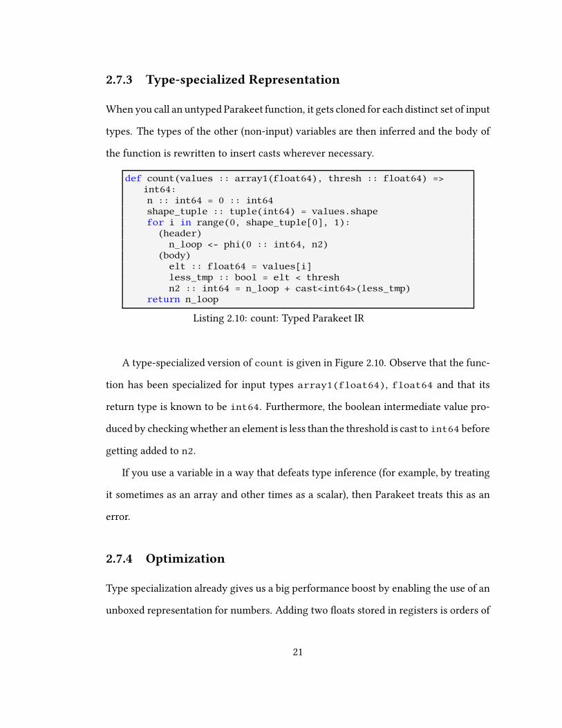
2.7.3 Type-specialized Representation
When you call an untyped Parakeet function, it gets cloned for each distinct set of input
types. The types of the other (non-input) variables are then inferred and the body of
the function is rewritten to insert casts wherever necessary.
def count(values :: array1(float64), thresh :: float64) =>int64:n :: int64 = 0 :: int64shape_tuple :: tuple(int64) = values.shapefor i in range(0, shape_tuple[0], 1):
(header)n_loop <- phi(0 :: int64, n2)
(body)elt :: float64 = values[i]less_tmp :: bool = elt < threshn2 :: int64 = n_loop + cast<int64>(less_tmp)
return n_loop
Listing 2.10: count: Typed Parakeet IR
A type-specialized version of count is given in Figure 2.10. Observe that the func-
tion has been specialized for input types array1(float64), float64 and that its
return type is known to be int64. Furthermore, the boolean intermediate value pro-
duced by checkingwhether an element is less than the threshold is cast to int64 before
getting added to n2.
If you use a variable in a way that defeats type inference (for example, by treating
it sometimes as an array and other times as a scalar), then Parakeet treats this as an
error.
2.7.4 Optimization
Type specialization already gives us a big performance boost by enabling the use of an
unboxed representation for numbers. Adding two �oats stored in registers is orders of
21
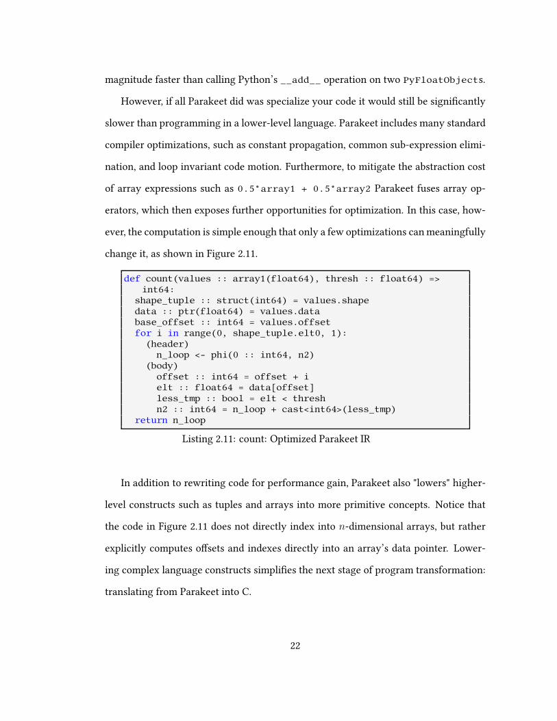
magnitude faster than calling Python’s __add__ operation on two PyFloatObjects.
However, if all Parakeet did was specialize your code it would still be signi�cantly
slower than programming in a lower-level language. Parakeet includes many standard
compiler optimizations, such as constant propagation, common sub-expression elimi-
nation, and loop invariant code motion. Furthermore, to mitigate the abstraction cost
of array expressions such as 0.5*array1 + 0.5*array2 Parakeet fuses array op-
erators, which then exposes further opportunities for optimization. In this case, how-
ever, the computation is simple enough that only a few optimizations canmeaningfully
change it, as shown in Figure 2.11.
def count(values :: array1(float64), thresh :: float64) =>int64:
shape_tuple :: struct(int64) = values.shapedata :: ptr(float64) = values.database_offset :: int64 = values.offsetfor i in range(0, shape_tuple.elt0, 1):
(header)n_loop <- phi(0 :: int64, n2)
(body)offset :: int64 = offset + ielt :: float64 = data[offset]less_tmp :: bool = elt < threshn2 :: int64 = n_loop + cast<int64>(less_tmp)
return n_loop
Listing 2.11: count: Optimized Parakeet IR
In addition to rewriting code for performance gain, Parakeet also "lowers" higher-
level constructs such as tuples and arrays into more primitive concepts. Notice that
the code in Figure 2.11 does not directly index into n-dimensional arrays, but rather
explicitly computes o�sets and indexes directly into an array’s data pointer. Lower-
ing complex language constructs simpli�es the next stage of program transformation:
translating from Parakeet into C.
22
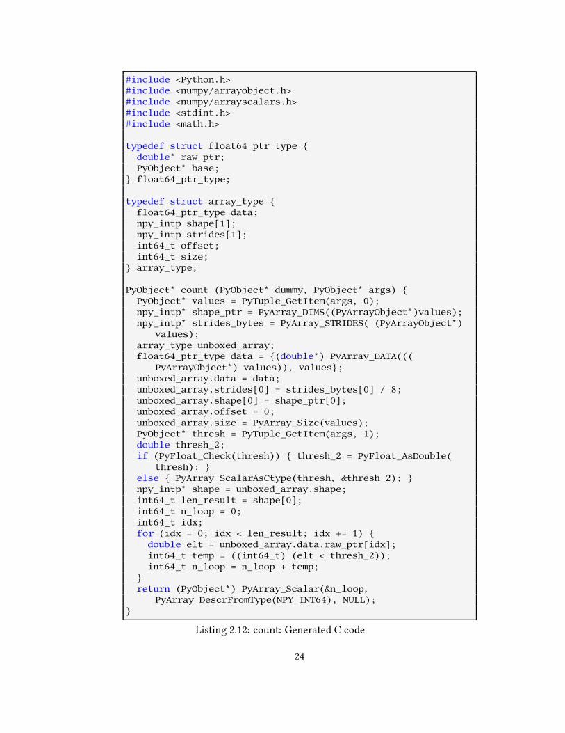
2.7.5 Generated C code
The translation from Parakeet’s lowered intermediate representation into C is largely
mechanical. Structured data types such as array descriptors and tuples become C
structs, which due to immutability assumptions can be safely passed by value. So that
this code can be used by the Python interpreter, the entry point into a compiled C func-
tion must extract all the input values from the Python interpreter’s PyObject repre-
sentation. Similarly, the result must be packaged up as a value the Python interpreter
understands. In between, however, the Python C API is not used. The C code for the
count function is shown in Listing 2.12. In this instance, it does not matter whether
the C, OpenMP, or CUDA backend was used, due to the lack of parallel operators in
the original program, all the backends generate largely identical output.
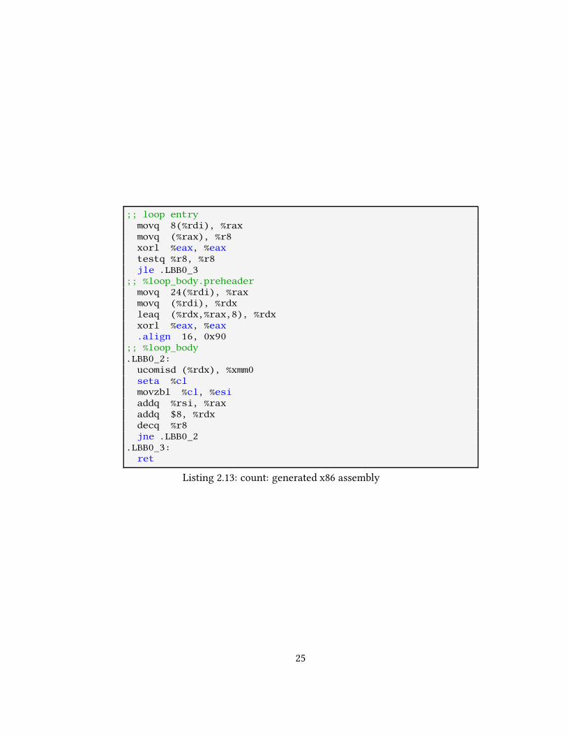
2.7.6 Generated x86 Assembly
Once we pass the torch to the C compiler, Parakeet’s job is mostly done. The external
compiler performs its own host of optimization passes on our code and, at last, we
arrive at native code. Shown in Figure 2.13 is the assembly generated for the main loop
from the code above.
Notice that we end up with the same number of machine instructions as we orig-
inally had Python bytecodes. It’s safe to suspect that the performance might have
somewhat improved.
2.7.7 Execution Times
In addition to benchmarking against the Python interpreter (an unfair comparisonwith
a predictable outcome), let’s also see Parakeet stacks up against an equivalent function
23
#include <Python.h>#include <numpy/arrayobject.h>#include <numpy/arrayscalars.h>#include <stdint.h>#include <math.h>
typedef struct float64_ptr_type {double* raw_ptr;PyObject* base;
} float64_ptr_type;
typedef struct array_type {float64_ptr_type data;npy_intp shape[1];npy_intp strides[1];int64_t offset;int64_t size;
} array_type;
PyObject* count (PyObject* dummy, PyObject* args) {PyObject* values = PyTuple_GetItem(args, 0);npy_intp* shape_ptr = PyArray_DIMS((PyArrayObject*)values);npy_intp* strides_bytes = PyArray_STRIDES( (PyArrayObject*)
values);array_type unboxed_array;float64_ptr_type data = {(double*) PyArray_DATA(((
PyArrayObject*) values)), values};unboxed_array.data = data;unboxed_array.strides[0] = strides_bytes[0] / 8;unboxed_array.shape[0] = shape_ptr[0];unboxed_array.offset = 0;unboxed_array.size = PyArray_Size(values);PyObject* thresh = PyTuple_GetItem(args, 1);double thresh_2;if (PyFloat_Check(thresh)) { thresh_2 = PyFloat_AsDouble(
thresh); }else { PyArray_ScalarAsCtype(thresh, &thresh_2); }npy_intp* shape = unboxed_array.shape;int64_t len_result = shape[0];int64_t n_loop = 0;int64_t idx;for (idx = 0; idx < len_result; idx += 1) {
double elt = unboxed_array.data.raw_ptr[idx];int64_t temp = ((int64_t) (elt < thresh_2));int64_t n_loop = n_loop + temp;
}return (PyObject*) PyArray_Scalar(&n_loop,
PyArray_DescrFromType(NPY_INT64), NULL);}
Listing 2.12: count: Generated C code
24
;; loop entrymovq 8(%rdi), %raxmovq (%rax), %r8xorl %eax, %eaxtestq %r8, %r8jle .LBB0_3
;; %loop_body.preheadermovq 24(%rdi), %raxmovq (%rdi), %rdxleaq (%rdx,%rax,8), %rdxxorl %eax, %eax.align 16, 0x90
;; %loop_body.LBB0_2:
ucomisd (%rdx), %xmm0seta %clmovzbl %cl, %esiaddq %rsi, %raxaddq $8, %rdxdecq %r8jne .LBB0_2
.LBB0_3:ret
Listing 2.13: count: generated x86 assembly
25
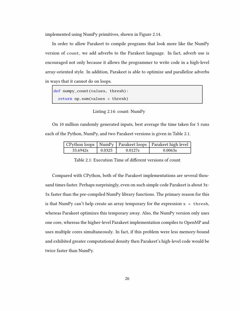
implemented using NumPy primitives, shown in Figure 2.14.
In order to allow Parakeet to compile programs that look more like the NumPy
version of count, we add adverbs to the Parakeet language. In fact, adverb use is
encouraged not only because it allows the programmer to write code in a high-level
array-oriented style. In addition, Parakeet is able to optimize and parallelize adverbs
in ways that it cannot do on loops.
def numpy_count(values, thresh):
return np.sum(values < thresh)
Listing 2.14: count: NumPy
On 10 million randomly generated inputs, best average the time taken for 5 runs
each of the Python, NumPy, and two Parakeet versions is given in Table 2.1.
CPython loops NumPy Parakeet loops Parakeet high level33.6942s 0.0325 0.0127s 0.0063s
Table 2.1: Execution Time of di�erent versions of count
Compared with CPython, both of the Parakeet implementations are several thou-
sand times faster. Perhaps surprisingly, even on such simple code Parakeet is about 3x-
5x faster than the pre-compiled NumPy library functions. The primary reason for this
is that NumPy can’t help create an array temporary for the expression x < thresh,
whereas Parakeet optimizes this temporary away. Also, the NumPy version only uses
one core, whereas the higher-level Parakeet implementation compiles to OpenMP and
uses multiple cores simultaneously. In fact, if this problem were less memory-bound
and exhibited greater computational density then Parakeet’s high-level code would be
twice faster than NumPy.
26
Chapter 3
History and Related Work
In the beginning, all computing was scienti�c computing. Early general purpose com-
puters such as the ENIAC [GG46] and MESM [FBB06] were commissioned to compute
artillery trajectories, simulate nuclear detonations, and crack cryptographic codes.
These machines required a tremendous expenditure of human e�ort to correctly con-
struct and encode their programs.
In the decade that followed, computers became widely available and better ab-
stractions for programming them were eagerly sought after. As a variety of program-
ming languages were devised, a tension became apparent between attaining e�ciency
through low-level control and the expressiveness of high-level abstractions. At the
broadest scope, it is possible to distinguish two lineages of philosophy in the design
of programming languages: (1) those whose features are carefully chosen to allow for
e�cient compilation and (2) abstract models of computation which optimize for pro-
grammer e�ciency and leave e�cient implementation as a secondary goal.
Programmers who adopted languages such as Fortran [BBB+57], CPL [BBH+63],
and Algol [NBB+63], demanded low-level control over data layout and program exe-
27
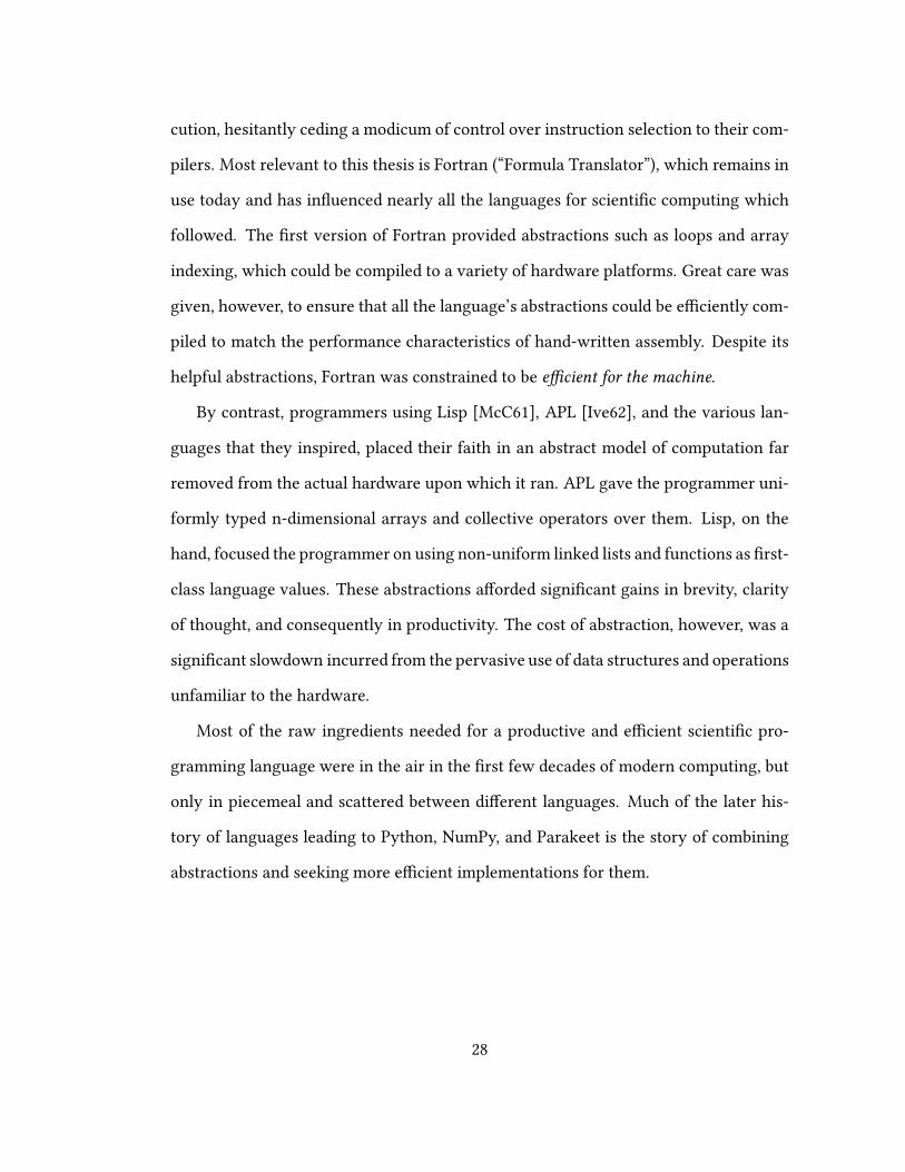
cution, hesitantly ceding a modicum of control over instruction selection to their com-
pilers. Most relevant to this thesis is Fortran (“Formula Translator”), which remains in
use today and has in�uenced nearly all the languages for scienti�c computing which
followed. The �rst version of Fortran provided abstractions such as loops and array
indexing, which could be compiled to a variety of hardware platforms. Great care was
given, however, to ensure that all the language’s abstractions could be e�ciently com-
piled to match the performance characteristics of hand-written assembly. Despite its
helpful abstractions, Fortran was constrained to be e�cient for the machine.
By contrast, programmers using Lisp [McC61], APL [Ive62], and the various lan-
guages that they inspired, placed their faith in an abstract model of computation far
removed from the actual hardware upon which it ran. APL gave the programmer uni-
formly typed n-dimensional arrays and collective operators over them. Lisp, on the
hand, focused the programmer on using non-uniform linked lists and functions as �rst-
class language values. These abstractions a�orded signi�cant gains in brevity, clarity
of thought, and consequently in productivity. The cost of abstraction, however, was a
signi�cant slowdown incurred from the pervasive use of data structures and operations
unfamiliar to the hardware.
Most of the raw ingredients needed for a productive and e�cient scienti�c pro-
gramming language were in the air in the �rst few decades of modern computing, but
only in piecemeal and scattered between di�erent languages. Much of the later his-
tory of languages leading to Python, NumPy, and Parakeet is the story of combining
abstractions and seeking more e�cient implementations for them.
28

3.1 Array Programming
I adopted the matrix algebra used in my thesis work, the systematic use of
matrices and higher-dimensional arrays (almost) learned in a course in Tensor
Analysis rashly taken in my third year at Queen’s, and (eventually) the notion
of Operators in the sense introduced by Heaviside in his treatment of Maxwell’s
equations.
— Kenneth E. Iverson
Array Programming is a paradigm wherein the primary data structure is an n-
dimensional array and algorithms are implemented chie�y through the creation, trans-
formation, and contraction of array values. These semantics were inspired by matrix
and tensor notation, but extended to collections of numbers without any particular
linear algebraic properties. The array programming paradigm was �rst introduced by
Kenneth Iverson’s APL [Ive62], which he conceived of as a “mathematical notation” as
much as a programming language.
APL uses an extremely terse syntaxwhich is richwith di�erent array operators. For
example, summing the numbers from 0 to 99 can be expressed in APL as+/ι100. Here
the �rst-order range operator “ι” is used to create a range of values and the higher-
order reduction operator / is combined with the �rst order addition function + to
express summation. Programming in APL makes extensive use of higher-order array
operators, or in the language’s native nomenclature, “adverbs”.
The basic programming paradigm embodied by APL inspired a lineage of many
other “pure” array languages, such as Nial [JGM86], Q [Bor08], and J [HI98]. The pri-
mary implementations for array languages have all tended to be simple interpreters,
relying on e�cient precompiled primitives for performance. The preference for inter-
preter implementations arises from the di�culty of assigning precise types to APL’s
29
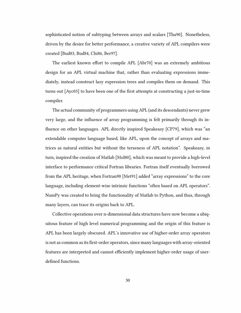
sophisticated notion of subtyping between arrays and scalars [Tha90]. Nonetheless,
driven by the desire for better performance, a creative variety of APL compilers were
created [Bud83, Bud84, Chi86, Ber97].
The earliest known e�ort to compile APL [Abr70] was an extremely ambitious
design for an APL virtual machine that, rather than evaluating expressions imme-
diately, instead construct lazy expression trees and compiles them on demand. This
turns out [Ayc03] to have been one of the �rst attempts at constructing a just-in-time
compiler.
The actual community of programmers using APL (and its descendants) never grew
very large, and the in�uence of array programming is felt primarily through its in-
�uence on other languages. APL directly inspired Speakeasy [CP79], which was “an
extendable computer language based, like APL, upon the concept of arrays and ma-
trices as natural entities but without the terseness of APL notation”. Speakeasy, in
turn, inspired the creation of Matlab [Mol80], which was meant to provide a high-level
interface to performance critical Fortran libraries. Fortran itself eventually borrowed
from the APL heritage, when Fortran90 [Met91] added “array expressions” to the core
language, including element-wise intrinsic functions “often based on APL operators”.
NumPy was created to bring the functionality of Matlab to Python, and thus, through
many layers, can trace its origins back to APL.
Collective operations over n-dimensional data structures have now become a ubiq-
uitous feature of high level numerical programming and the origin of this feature is
APL has been largely obscured. APL’s innovative use of higher-order array operators
is not as common as its �rst-order operators, sincemany languageswith array-oriented
features are interpreted and cannot e�ciently implement higher-order usage of user-
de�ned functions.
30
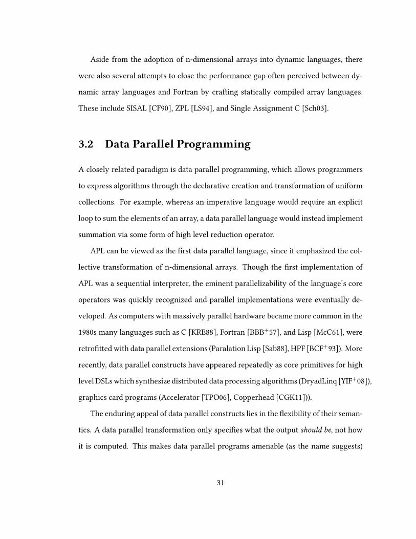
Aside from the adoption of n-dimensional arrays into dynamic languages, there
were also several attempts to close the performance gap often perceived between dy-
namic array languages and Fortran by crafting statically compiled array languages.
These include SISAL [CF90], ZPL [LS94], and Single Assignment C [Sch03].
3.2 Data Parallel Programming
A closely related paradigm is data parallel programming, which allows programmers
to express algorithms through the declarative creation and transformation of uniform
collections. For example, whereas an imperative language would require an explicit
loop to sum the elements of an array, a data parallel languagewould instead implement
summation via some form of high level reduction operator.
APL can be viewed as the �rst data parallel language, since it emphasized the col-
lective transformation of n-dimensional arrays. Though the �rst implementation of
APL was a sequential interpreter, the eminent parallelizability of the language’s core
operators was quickly recognized and parallel implementations were eventually de-
veloped. As computers with massively parallel hardware becamemore common in the
1980s many languages such as C [KRE88], Fortran [BBB+57], and Lisp [McC61], were
retro�tted with data parallel extensions (Paralation Lisp [Sab88], HPF [BCF+93]). More
recently, data parallel constructs have appeared repeatedly as core primitives for high
levelDSLswhich synthesize distributed data processing algorithms (DryadLinq [YIF+08]),
graphics card programs (Accelerator [TPO06], Copperhead [CGK11])).
The enduring appeal of data parallel constructs lies in the �exibility of their seman-
tics. A data parallel transformation only speci�es what the output should be, not how
it is computed. This makes data parallel programs amenable (as the name suggests)
31

to parallelization, both in terms of coarse-grained data partitioning and �ne-grained
SIMD vectorization. In addition, the algebraic nature of data parallel operators allows
for dramatic restructuring of the program in order to improve performance. Most com-
monly, data parallel operators can be fused by applying simple syntactic rewrite rules
which results in the elimination of synchronization points, increased computational
density, and signi�cant gains in performance.
3.2.1 Collection-Oriented Languages
Another closely paradigm closely related to both array programming and data par-
allel programming is that of collection-oriented languages. By the mid-1980’s, there
was a widespread proliferation of high level languages which relied on some privi-
leged collection type as a central mechanism by which programs could be expressed.
These included array-oriented languages of the APL family, the set-oriented language
SETL [SDSD86], as well as Lisp dialects which used either conventional lists or other
more exotic data structures such as distributed mappings [SJH86]. What such lan-
guages have in common is at minimum, an apply-to-each operation which implicitly
traverses a collection (as well as often some form of reductions and scans).
Their similarities were documented by Sipelstein and Blelloch in a review named
"Collection Oriented Langauges" [SB91]. Blelloch focuses on the pervasive use of
data parallel operators such as Map and Reduce, though sometimes named di�er-
ently or entirely disguised behind the semantics of implicit elementwise function ap-
plication. This work seems to have inspired Blelloch’s nested data parallel language
NESL [BCH+94].
The data parallel programming model allows programmers to express algorithms
through the declarative creation and transformation of uniform collections. For ex-
32
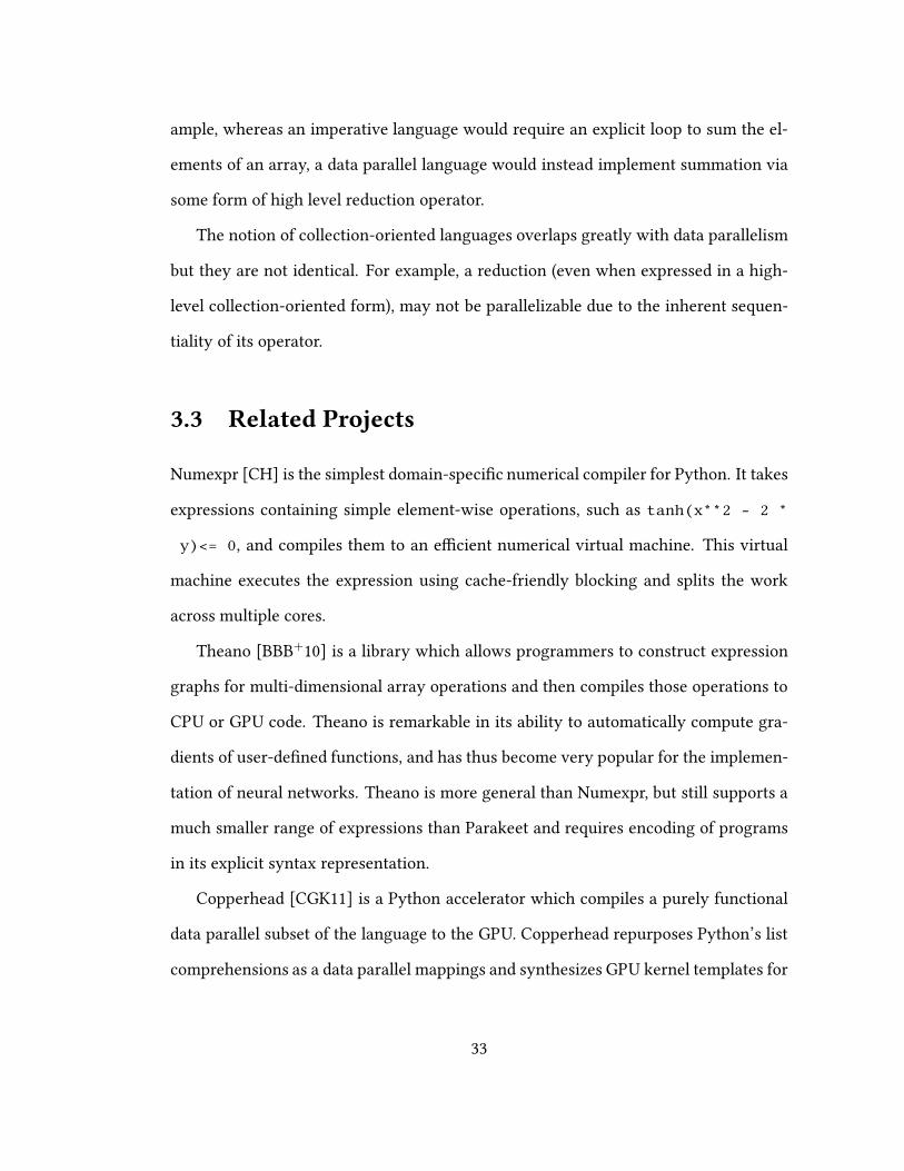
ample, whereas an imperative language would require an explicit loop to sum the el-
ements of an array, a data parallel language would instead implement summation via
some form of high level reduction operator.
The notion of collection-oriented languages overlaps greatly with data parallelism
but they are not identical. For example, a reduction (even when expressed in a high-
level collection-oriented form), may not be parallelizable due to the inherent sequen-
tiality of its operator.
3.3 Related Projects
Numexpr [CH] is the simplest domain-speci�c numerical compiler for Python. It takes
expressions containing simple element-wise operations, such as tanh(x**2 - 2 *
y)<= 0, and compiles them to an e�cient numerical virtual machine. This virtual
machine executes the expression using cache-friendly blocking and splits the work
across multiple cores.
Theano [BBB+10] is a library which allows programmers to construct expression
graphs for multi-dimensional array operations and then compiles those operations to
CPU or GPU code. Theano is remarkable in its ability to automatically compute gra-
dients of user-de�ned functions, and has thus become very popular for the implemen-
tation of neural networks. Theano is more general than Numexpr, but still supports a
much smaller range of expressions than Parakeet and requires encoding of programs
in its explicit syntax representation.
Copperhead [CGK11] is a Python accelerator which compiles a purely functional
data parallel subset of the language to the GPU. Copperhead repurposes Python’s list
comprehensions as a data parallel mappings and synthesizes GPU kernel templates for
33
operators such as map and reduce. Copperhead is limited by its inability to express
local mutable variables and array expressions. Parakeet can be seen as an extension of
Copperhead’s ideas to a much larger swath of idiomatic programming constructs.
Pythran [GBA13] is a compiler for numerical Python which achieves impressive
performance by generating multi-core programs using OpenMP. It di�ers from Para-
keet in that it is a static compiler which requires user annotations.
Numba [Con] is the closest project to Parakeet in both its aims and internal ma-
chinery. Like Parakeet, Numba provides a function decorator which intercepts func-
tion calls and uses argument types as the basis for type specialization. Numba then
compiles type specialized programs to LLVM. Numba relies on loops for performance
sensitive code, and lacks any concept analogous to Parakeet’s higher order data parallel
operators.
34
Chapter 4
Parakeet’s Intermediate
Representation
Parakeet uses a tree-structured intermediate representation where every function’s
body is a sequence of statements. Statements corresponding to loops and branches
may in turn contain their own nested sequences of statements. All control �ow in
Parakeet must be “structured”, meaning it is impossible to express arbitrary jumps be-
tween disparate parts of a program. Each structured control statement tracks the data
�ow arising from branching using SSA [CFR+89] Φ-nodes at merge points. This com-
bination is reminiscent of Oberon’s Structured SSA [BM94], which is easier to analyze
and rewrite but makes it di�cult to express constructs such as Python’s break and
continue.
When a Python function is �rst encountered by Parakeet, it is translated into Para-
keet’s intermediate representation but without any type annotations. This syntax rep-
resentation acts as an untyped function template, giving rise to multiple distinct typed
instantiations for each distinct set of input types. Later, when specializing this untyped
35
template for particular input types, all syntax nodes are annotated with types and any
source of type ambiguity or potential dynamicism is translated into explicit coercions.
The two major transformations which must be performed while converting from
Python’s syntrax into Parakeet’s intermediate representation are:
• SSA Conversion. Each assignment to the same variable name is given a distinct
name. At places where a variable might take its value from multiple renamed
source (control �ow merge arising from loops and branches) explicit Φ-nodes
track the �ow of values. In Parakeet, these nodes are represented as a collection
of bindings such as xi = φ(eleft, eright), where the value of xi is selected depending
on which branch was taken.
• Lambda Lifting [Joh85] & Closure Conversion [Rey72]. Rather than allow
nested function de�nitions as statements, Parakeet gives each function a unique
identity by lifting it to the top-level scope. Any values which a de�nition closed
over are added as formal parameters and where the de�nition originally took
place a closure object is constructed instead.
4.1 Simple Expressions
This section enumerates the Parakeet expressions which are unrelated to the construc-
tion, transformation, and inspection of array values. This includes creating scalar val-
ues, tuples, closures, and slices.
• Const(value)
Constants can be booleans, signed or unsigned integers, �oating point values, or
the None object.
36
• Var(name)
Variables in Parakeet’s intermediate representation must originate from a local
binding either as the input argument to a function, a single assignment state-
ment, or a φ-node associated with some control �ow statement.
• PrimCall(prim, x1, . . . xn)
Parakeet’s primitives are basic math operators such as add or divide, logical
operators such as logical_and, or transcendental math functions such as exp
or sin.
• Select(cond , trueValue , falseValue)
Returns trueValue when cond is true, and falseValue otherwise.
• Tuple(x1, . . . , xn)
Construct an n-element tuple object from the individual values x1, . . . , xn.
• TupleElt(x, i)
Extract the ith element of x. The index i must be a �xed constant and not a
dynamically varying expression. Can be denoted more compactly as xi.
• Closure(f , x1, . . . , xn)
Partially apply the arguments x1, . . . , xn to the function f , which must have
at least n + 1 inputs. The result is a closure object, which can be called like a
function.
• ClosureElt(clos, i)
Extract the ith partially applied argument from the closure value clos. The index
i must be a �xed constant and not a dynamically varying expression. Can be
denoted more compactly as clos i.
37
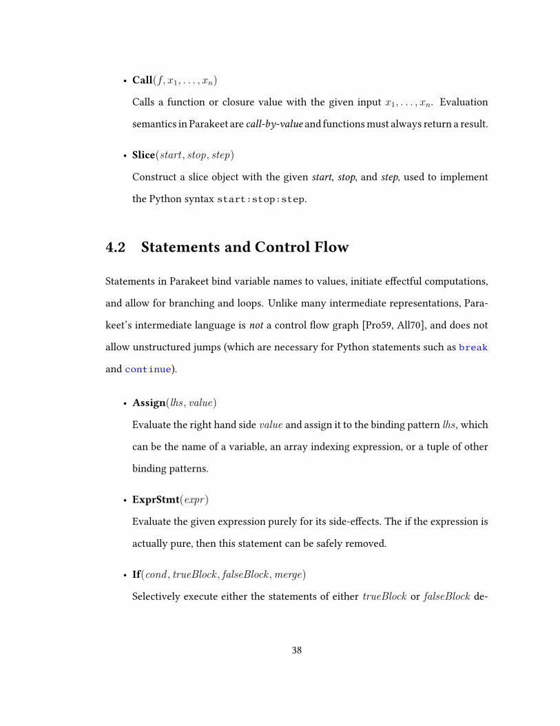
• Call(f, x1, . . . , xn)
Calls a function or closure value with the given input x1, . . . , xn. Evaluation
semantics in Parakeet are call-by-value and functionsmust always return a result.
• Slice(start , stop, step)
Construct a slice object with the given start, stop, and step, used to implement
the Python syntax start:stop:step.
4.2 Statements and Control Flow
Statements in Parakeet bind variable names to values, initiate e�ectful computations,
and allow for branching and loops. Unlike many intermediate representations, Para-
keet’s intermediate language is not a control �ow graph [Pro59, All70], and does not
allow unstructured jumps (which are necessary for Python statements such as break
and continue).
• Assign(lhs , value)
Evaluate the right hand side value and assign it to the binding pattern lhs , which
can be the name of a variable, an array indexing expression, or a tuple of other
binding patterns.
• ExprStmt(expr)
Evaluate the given expression purely for its side-e�ects. The if the expression is
actually pure, then this statement can be safely removed.
• If(cond , trueBlock , falseBlock ,merge)
Selectively execute either the statements of either trueBlock or falseBlock de-
38
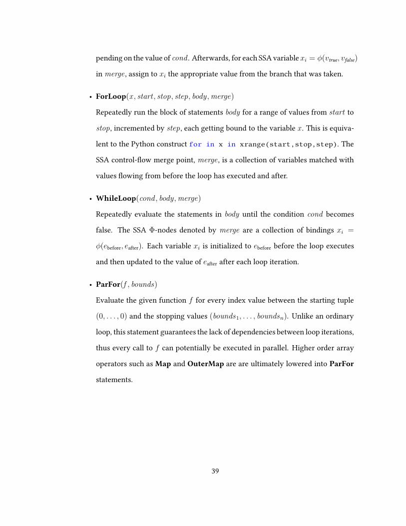
pending on the value of cond . Afterwards, for each SSA variablexi = φ(vtrue, vfalse)
in merge , assign to xi the appropriate value from the branch that was taken.
• ForLoop(x , start , stop, step, body ,merge)
Repeatedly run the block of statements body for a range of values from start to
stop, incremented by step, each getting bound to the variable x . This is equiva-
lent to the Python construct for in x in xrange(start,stop,step). The
SSA control-�ow merge point, merge , is a collection of variables matched with
values �owing from before the loop has executed and after.
• WhileLoop(cond , body,merge)
Repeatedly evaluate the statements in body until the condition cond becomes
false. The SSA Φ-nodes denoted by merge are a collection of bindings xi =
φ(ebefore, eafter). Each variable xi is initialized to ebefore before the loop executes
and then updated to the value of eafter after each loop iteration.
• ParFor(f , bounds)
Evaluate the given function f for every index value between the starting tuple
(0, . . . , 0) and the stopping values (bounds1, . . . , boundsn). Unlike an ordinary
loop, this statement guarantees the lack of dependencies between loop iterations,
thus every call to f can potentially be executed in parallel. Higher order array
operators such as Map and OuterMap are are ultimately lowered into ParFor
statements.
39
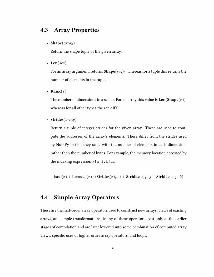
4.3 Array Properties
• Shape(array)
Return the shape tuple of the given array.
• Len(seq)
For an array argument, returns Shape(seq)0, whereas for a tuple this returns the
number of elements in the tuple.
• Rank(x )
The number of dimensions in a scalar. For an array this value is Len(Shape(x)),
whereas for all other types the rank if 0.
• Strides(array)
Return a tuple of integer strides for the given array. These are used to com-
pute the addresses of the array’s elements. These di�er from the strides used
by NumPy in that they scale with the number of elements in each dimension,
rather than the number of bytes. For example, the memory location accessed by
the indexing expression x[a,j,k] is:
base(x) + itemsize(x) · (Strides(x)0 · i+ Strides(x)1 · j + Strides(x)2 · k)
4.4 Simple Array Operators
These are the �rst-order array operators used to construct new arrays, views of existing
arrays, and simple transformations. Many of these operators exist only at the earlier
stages of compilation and are later lowered into some combination of computed array
views, speci�c uses of higher order array operators, and loops.
40
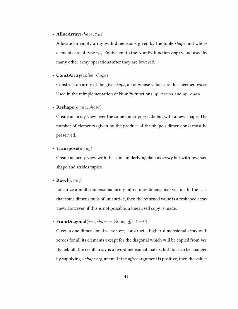
• AllocArray(shape, τelt)
Allocate an empty array with dimensions given by the tuple shape and whose
elements are of type τelt. Equivalent to the NumPy function empty and used by
many other array operations after they are lowered.
• ConstArray(value, shape)
Construct an array of the give shape, all of whose values are the speci�ed value.
Used in the reimplementation of NumPy functions np.zeros and np.ones.
• Reshape(array , shape)
Create an array view over the same underlying data but with a new shape. The
number of elements (given by the product of the shape’s dimensions) must be
preserved.
• Transpose(array)
Create an array view with the same underlying data as array but with reversed
shape and strides tuples.
• Ravel(array)
Linearize a multi-dimensional array into a one-dimensional vector. In the case
that some dimension is of unit stride, then the returned value is a reshaped array
view. However, if this is not possible, a linearized copy is made.
• FromDiagonal(vec, shape = None, offset = 0)
Given a one-dimensional vector vec, construct a higher-dimensional array with
zeroes for all its elements except for the diagonal which will be copied from vec.
By default, the result array is a two-dimensional matrix, but this can be changed
by supplying a shape argument. If the o�set argument is positive, then the values
41
of vec are copied into a diagonal above the main diagonal. If it’s negative, then
vec gets copied below the main diagonal.
• ExtractDiagonal(array , offset = 0)
Given a multidimensional array, return a vector containing the values of its di-
agonal entries array[i+ offset , . . . , i+ offset ].
• Tile(array , reps)
Repeat the contents of the given array as many times along dimension i as given
in the tuple element repsi. If Len(reps) < Rank(array) then extra 1s are used to
extend reps from the left. Similarly, if Len(reps) > Rank(array) then the shape
of the array is extended with 1s.
4.5 Memory Allocation
These constructs are accessible to the programmer but are rather used by later stages
of the compilation pipeline.
• Alloc(n, τ).
Returns a pointer to a freshly allocated data bu�er with n elements of type τ ,
whose size in bytes is itemsize(τ) · n.
• Free(ptr).
Manually deallocate the data bu�er at address ptr.
• ArrayView(data, τ, shape, strides, o�set)
Create an array view over the memory address range (data + o�set) : (data +
o�set + itemsize(τ) · Πishapei). Its shape is given by the tuple argument shape
and the array strides by the tuple argument strides.
42
4.6 Higher Order Array Operators
Parakeet’s representation of its data parallel operations di�ers from traditional presen-
tations in several ways.
Diversity. The biggest distinction between Parakeet and other languages which
use data parallel operators, is the dizzying menagerie of operators that Para-
keet uses internally. Many languages include generalMap and Reduce functions,
and a few even have something resembling a higher-order pre�x-scan. Parakeet,
however, also uses many other operators such as OuterMap, IndexMap, IndexRe-
duce, and Filter. None of these operators are essential, in the sense that you could
reimplement them using some combination of �rst order array constructors and
nestings of some smaller core set of higher order operators. However, in the ab-
sence of any other forms of abstract iteration, a minimalist approach results in
missed opportunities for array optimizations and sub-par performance.
Multiple Array Arguments. Data parallel operators are often presented as
consuming a single collection, which is often combined with �rst-order opera-
tors such as zip that combine the elements of multiple collections. Parakeet, on
the other, allows array operators to consume multiple array arguments directly.
Arguments can even di�er in dimensionality, so that Map(f, matrix, vector, axis
= 0) would call f with every row in matrix and every element in vector.
Axis of Traversal. Since the primary data type in Parakeet is an n-dimensional
array (and not some sort of �at sequence or stream) it is necessary for data par-
allel operators know which dimension(s) they should traverse. This is captured
with the axis property of every operator, which is either an integer constant indi-
43
cating a single dimension or the wildcard None, means that the operator should
apply to every scalar element.
Additional Function Parameters. It is typical for operators such as Reduce
and Scan to be speci�ed using only a binary operator. However, this approach
breaks down with multiple array arguments. It is necessary to also specify a
transformationwhichmaps from elements of the input arrays to the accumulator
type. Additionally, Scan is equipped with an emit function which transforms
from the accumulator type to some potentially di�erent output type.
4.6.1 Mapping Operations
• Map(f, X1, ...,Xn, axis = None)
Apply the function f to each element of the array arguments. By default, the
value of axis argument is None, which means that every call to f is given scalar
elements of the array arguments. If the axis keyword is set to some integer value,
then the arguments to f will be slices along that dimension of all the arrays. This
can be used, for example, for applying f to all columns or rows of a matrix.
• OuterMap(f, X1, . . . , Xn, axis = 0). Apply the function f to all combinations
of elements between the input arrays.
• Filter(f, pred, X1, . . . , Xn, axis = 0).
For the aligned input elements X1, . . . , Xn, construct an array from the results
of f(x1, . . . , xn) when pred(x1, . . . , xn) is true and discard the values for which
the predicate is false.
• IndexMap(f, shape).
44
Similar to aMap but evaluates the function f for every index tuple in the iteration
space from 0, . . . , 0 to σ1, . . . , σn.
• IndexFilter(f, pred, shape). Similar to IndexMap but uses the predicate func-
tion pred to exclude index combinations.
4.6.2 Reductions
• Reduce(f,⊕, X1, . . . , Xn, init = None, axis = None)
Combine all the elements of the array arguments using the (n+ 1)-ary commu-
tative function f . The init keyword is an optional initial value for the reduction.
Examples of reductions are the NumPy functions sum and product.
• IndexReduce(f,⊕, shape) Performs a reduction across the index space from
(0, . . . , 0) to the bounds (shape1, . . . , shape
n). The function argument f converts
from an input index (i1, . . . , in) into a value compatible with combine operation
⊕.
• FilterReduce(f,⊕, pred, X1 . . .Xn). Filter the elements of the input arrays us-
ing the function pred, transform the surviving elementswith f and combine them
into a single result with the binary function ⊕.
• IndexFilterReduce(f,⊕, pred, X1 . . . Xn).
4.6.3 Scans
• Scan(f,⊕, emit, X1, . . . , Xn, init = None, axis = None)
Combine all the elements of the array arguments and return an array containing
45
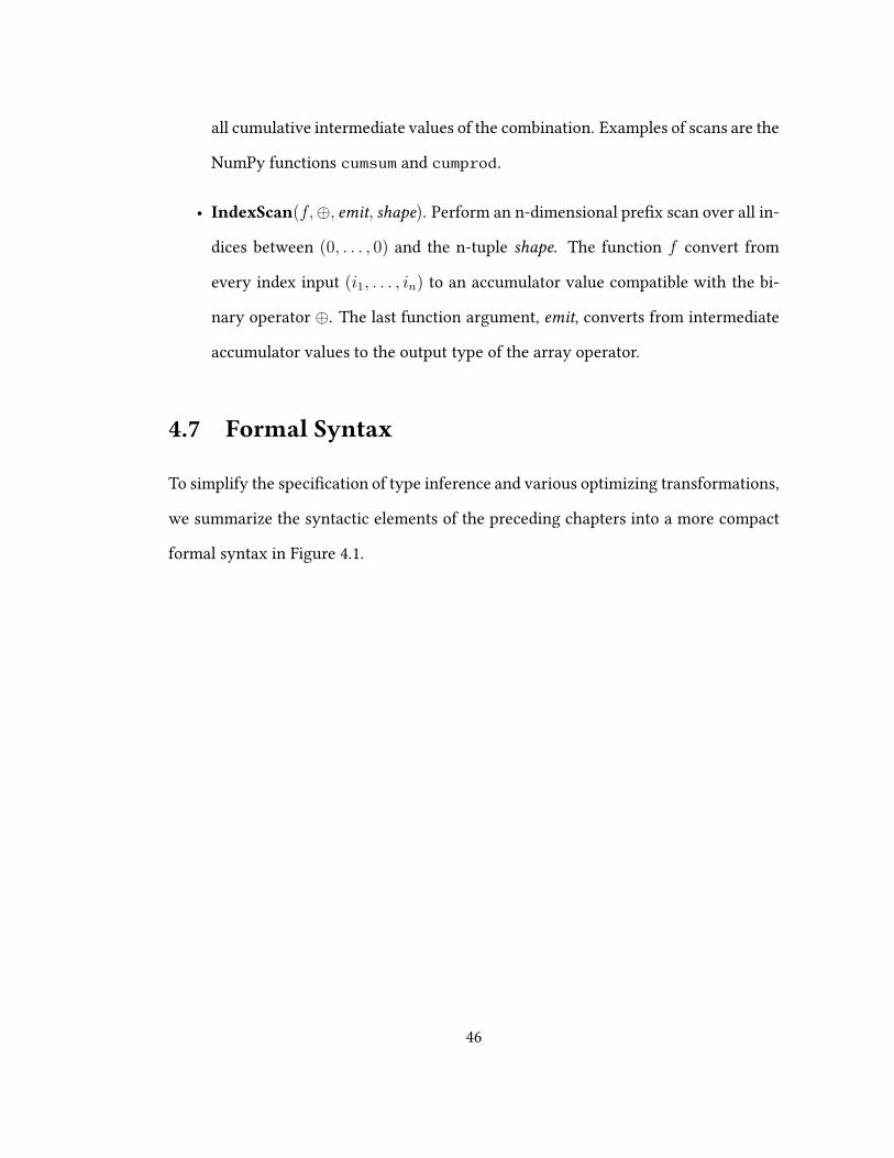
all cumulative intermediate values of the combination. Examples of scans are the
NumPy functions cumsum and cumprod.
• IndexScan(f,⊕, emit, shape). Perform an n-dimensional pre�x scan over all in-
dices between (0, . . . , 0) and the n-tuple shape. The function f convert from
every index input (i1, . . . , in) to an accumulator value compatible with the bi-
nary operator ⊕. The last function argument, emit, converts from intermediate
accumulator values to the output type of the array operator.
4.7 Formal Syntax
To simplify the speci�cation of type inference and various optimizing transformations,
we summarize the syntactic elements of the preceding chapters into a more compact
formal syntax in Figure 4.1.
46
function f ::= λx1, ... , xn.s+
statement s ::= x = e | x[eidx]= e
| expr e| return e
| if e then s+ else s+ merge Φ+
| while econd do s+ merge Φ+
| for x in (estart, estop, estep) do s+ merge Φ+
| parfor(ef , ebounds)
SSA merge Φ ::= x = φ(eleft, eright)
expression e ::= x | const | prim(e1, . . . , en)| e1 × . . .× en | proj(etuple, i)
| [e1, . . . , en] | earray[eidx]| none | slice(estart, estop, estep)| closure(f, e1, . . . , ek)
| ef(e1, . . . , ek)|Mapα(ef , e1, . . . , en)
| OuterMapα(ef , e1, . . . , en)| Filterα(ef , epred, eresult, e1, . . . , en)
| Reduceα(ef , e⊕, einit?, e1, . . . , en)| FilterReduceα(ef , e⊕, epred, einit?, e1, . . . , en)| Scanα(ef , e⊕, e emit, einit?, e1, . . . , en)
| IndexMap(ef , eσ)| IndexReduce(ef , e⊕, einit?, eσ)
| IndexFilterReduce(ef , epred, e⊕, einit?, eσ)| IndexScan(ef , e⊕, eemit, einit?, eσ)
Figure 4.1: Parakeet’s Internal Syntax
47
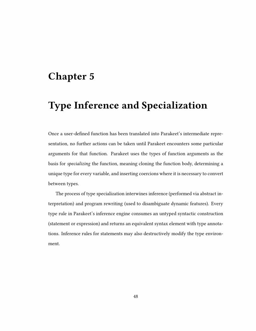
Chapter 5
Type Inference and Specialization
Once a user-de�ned function has been translated into Parakeet’s intermediate repre-
sentation, no further actions can be taken until Parakeet encounters some particular
arguments for that function. Parakeet uses the types of function arguments as the
basis for specializing the function, meaning cloning the function body, determining a
unique type for every variable, and inserting coercions where it is necessary to convert
between types.
The process of type specialization interwines inference (performed via abstract in-
terpretation) and program rewriting (used to disambiguate dynamic features). Every
type rule in Parakeet’s inference engine consumes an untyped syntactic construction
(statement or expression) and returns an equivalent syntax element with type annota-
tions. Inference rules for statements may also destructively modify the type environ-
ment.
48

5.1 Type System
Parakeet’s type system (Figure 5.1) is limited to scalars, n-dimensional arrays of scalar
elements, tuples of arbitrary values, slice values, a singleton None object, and type val-
ues (used to represent the dtype arguments of NumPy functions). This small collection
of possible types is su�cient for a large subset of the NumPy library functions. Notably
missing is support for complex numbers structured array elements, various array iter-
ators and grids, all of which would be necessary for a full-featured reimplementation
of NumPy.
scalar s ::= int8 | int16 | int32 | int64 |uint8 | uint16 | uint32 | uint64 |�oat32 | �oat64 | bool
type τ ::= s | array(s, k) | slice | none | τ1 × ... × τn |closure(f , τ1 × ... × τn) | typeval(s)
Figure 5.1: Types
Parakeet’s type system has a rich subtype structure, implementing both the scalar
hierarchy of NumPy (Figure 5.2) and broadcasting/rank polymorphism [Sch03]. Sub-
typing is implemented by inserting coercions [BTCGS91] into the rewritten typed rep-
resentation of a function. These coercions can be simple casts between scalar values
or Map operators which eliminate array-oriented polymorphism.
49
bool
uint8
uint16
uint32
uint64
int8
int16
int32
int64 �oat32
�oat64
Figure 5.2: Scalar Subtype Hierarchy
5.2 Type Specialization Algorithm
Parakeet’s type specializer is presented here in a stylized form as a set of mutually
recursive rewrite rules. The entry point into specialization is S(f, τ1, . . . , τn), de�ned
in Algorithm 5.1, which takes an untyped function and a sequence of input types, and
returns a rewritten type-specialized version of the function. If the function argument
to S is a closure rather than a bare function, then the underlying function is extracted
and the types of the closed-over arguments are prepended to the sequence of input
types.
The case-speci�c logic of specializing each kind of statement and expression in
Parakeet’s intermediate language is encompassed by the J·KE operation. The sub-
scripted E represents the accumulated type environment at the point where each syn-
tactic construct is encountered. A variety of helper functions (shown in Figure 5.3)
50
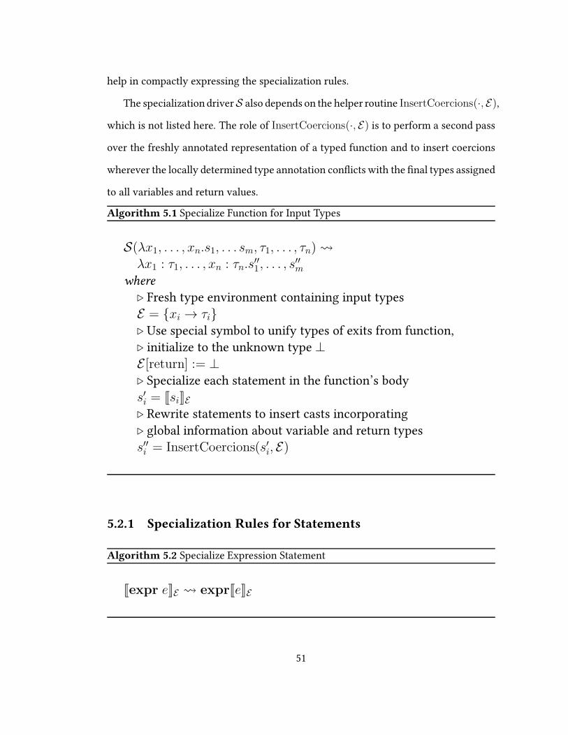
help in compactly expressing the specialization rules.
The specialization driverS also depends on the helper routine InsertCoercions(·, E),
which is not listed here. The role of InsertCoercions(·, E) is to perform a second pass
over the freshly annotated representation of a typed function and to insert coercions
wherever the locally determined type annotation con�icts with the �nal types assigned
to all variables and return values.
Algorithm 5.1 Specialize Function for Input Types
S(λx1, . . . , xn.s1, . . . sm, τ1, . . . , τn) λx1 : τ1, . . . , xn : τn.s
′′1, . . . , s
′′m
where
⊲ Fresh type environment containing input typesE = {xi → τi}⊲ Use special symbol to unify types of exits from function,⊲ initialize to the unknown type ⊥E [return] := ⊥⊲ Specialize each statement in the function’s bodys′i = JsiKE⊲ Rewrite statements to insert casts incorporating⊲ global information about variable and return typess′′i = InsertCoercions(s′i, E)
5.2.1 Specialization Rules for Statements
Algorithm 5.2 Specialize Expression Statement
Jexpr eKE exprJeKE
51
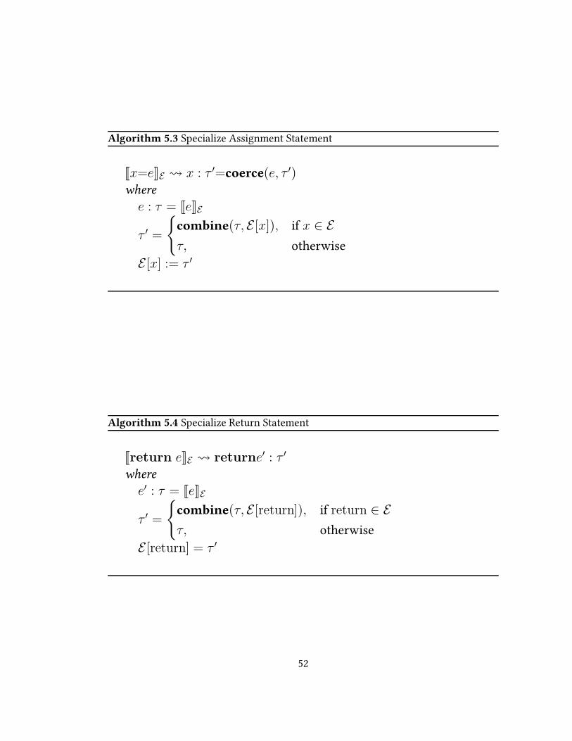
Algorithm 5.3 Specialize Assignment Statement
Jx=eKE x : τ ′=coerce(e, τ ′)where
e : τ = JeKE
τ ′ =
{
combine(τ, E [x]), if x ∈ E
τ, otherwise
E [x] := τ ′
Algorithm 5.4 Specialize Return Statement
Jreturn eKE returne′ : τ ′
where
e′ : τ = JeKE
τ ′ =
{
combine(τ, E [return]), if return ∈ E
τ, otherwise
E [return] = τ ′
52
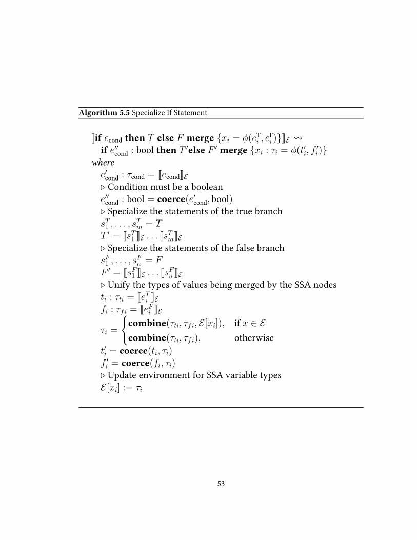
Algorithm 5.5 Specialize If Statement
Jif econd then T else F merge {xi = φ(eTi , eFi )}KE
if e′′cond : bool then T ′else F ′ merge {xi : τi = φ(t′i, f′i)}
where
e′cond : τcond = JecondKE⊲ Condition must be a booleane′′cond : bool = coerce(e′cond, bool)⊲ Specialize the statements of the true branchsT1 , . . . , s
Tm = T
T ′ = JsT1 KE . . . JsTmKE
⊲ Specialize the statements of the false branchsF1 , . . . , s
Fn = F
F ′ = JsF1 KE . . . JsFn KE
⊲ Unify the types of values being merged by the SSA nodesti : τti = JeTi KEfi : τfi = JeFi KE
τi =
{
combine(τti, τfi, E [xi]), if x ∈ E
combine(τti, τfi), otherwise
t′i = coerce(ti, τi)
f ′i = coerce(fi, τi)⊲ Update environment for SSA variable typesE [xi] := τi
53
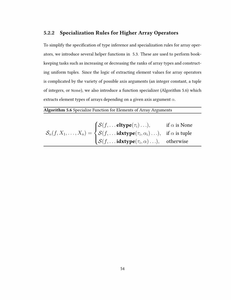
5.2.2 Specialization Rules for Higher Array Operators
To simplify the speci�cation of type inference and specialization rules for array oper-
ators, we introduce several helper functions in 5.3. These are used to perform book-
keeping tasks such as increasing or decreasing the ranks of array types and construct-
ing uniform tuples. Since the logic of extracting element values for array operators
is complicated by the variety of possible axis arguments (an integer constant, a tuple
of integers, or None), we also introduce a function specializer (Algorithm 5.6) which
extracts element types of arrays depending on a given axis argument α.
Algorithm 5.6 Specialize Function for Elements of Array Arguments
Sα(f,X1, . . . , Xn) =
S(f, . . . eltype(τi) . . .), if α is None
S(f, . . . idxtype(τi, αi) . . .), if α is tuple
S(f, . . . idxtype(τi, α) . . .), otherwise
54
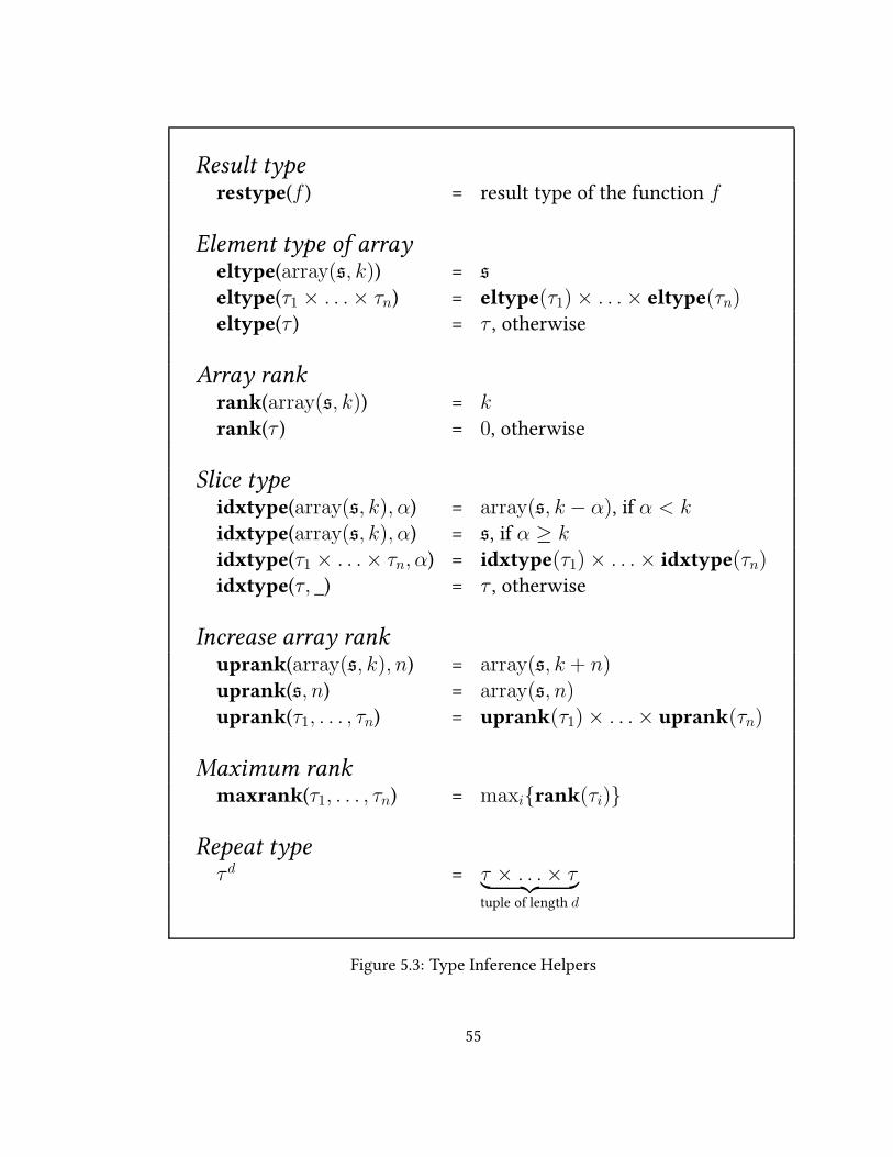
Result typerestype(f ) = result type of the function f
Element type of arrayeltype(array(s, k)) = s
eltype(τ1 × . . .× τn) = eltype(τ1)× . . .× eltype(τn)eltype(τ ) = τ , otherwise
Array rankrank(array(s, k)) = k
rank(τ ) = 0, otherwise
Slice typeidxtype(array(s, k), α) = array(s, k − α), if α < k
idxtype(array(s, k), α) = s, if α ≥ kidxtype(τ1 × . . .× τn, α) = idxtype(τ1)× . . .× idxtype(τn)idxtype(τ, _) = τ , otherwise
Increase array rankuprank(array(s, k), n) = array(s, k + n)uprank(s, n) = array(s, n)
uprank(τ1, . . . , τn) = uprank(τ1)× . . .× uprank(τn)
Maximum rankmaxrank(τ1, . . . , τn) = maxi{rank(τi)}
Repeat typeτ d = τ × . . .× τ
︸ ︷︷ ︸
tuple of length d
Figure 5.3: Type Inference Helpers
55
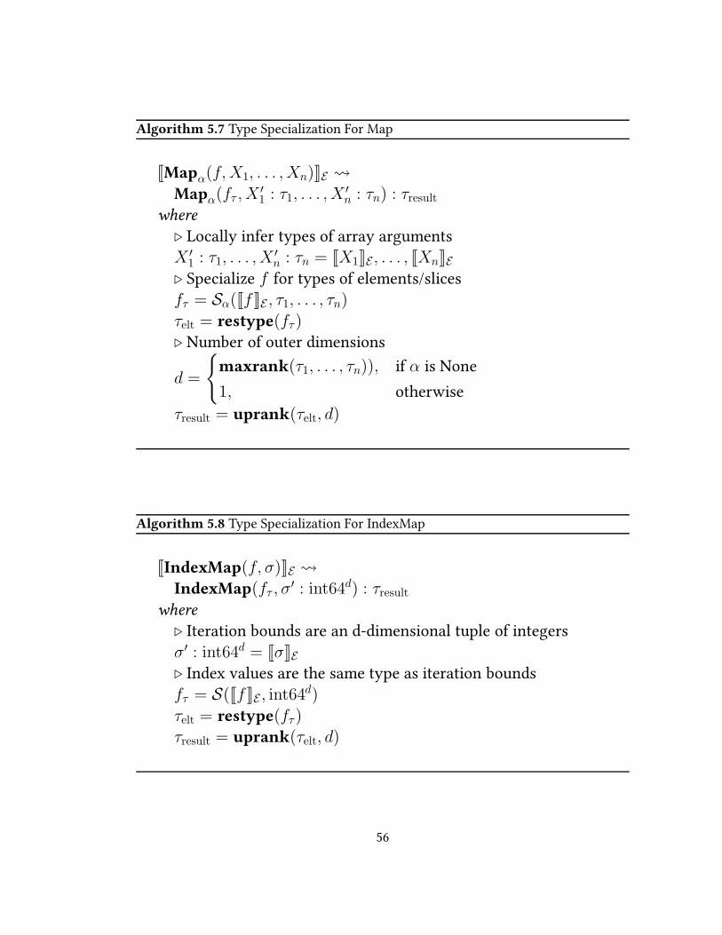
Algorithm 5.7 Type Specialization For Map
JMapα(f,X1, . . . , Xn)KE
Mapα(fτ , X′1 : τ1, . . . , X
′n : τn) : τresult
where
⊲ Locally infer types of array argumentsX ′
1 : τ1, . . . , X′n : τn = JX1KE , . . . , JXnKE
⊲ Specialize f for types of elements/slicesfτ = Sα(JfKE , τ1, . . . , τn)
τelt = restype(fτ)⊲ Number of outer dimensions
d =
{
maxrank(τ1, . . . , τn)), if α is None
1, otherwise
τresult = uprank(τelt, d)
Algorithm 5.8 Type Specialization For IndexMap
JIndexMap(f, σ)KE IndexMap(fτ , σ
′ : int64d) : τresultwhere
⊲ Iteration bounds are an d-dimensional tuple of integersσ′ : int64d = JσKE⊲ Index values are the same type as iteration boundsfτ = S(JfKE , int64
d)
τelt = restype(fτ)τresult = uprank(τelt, d)
56
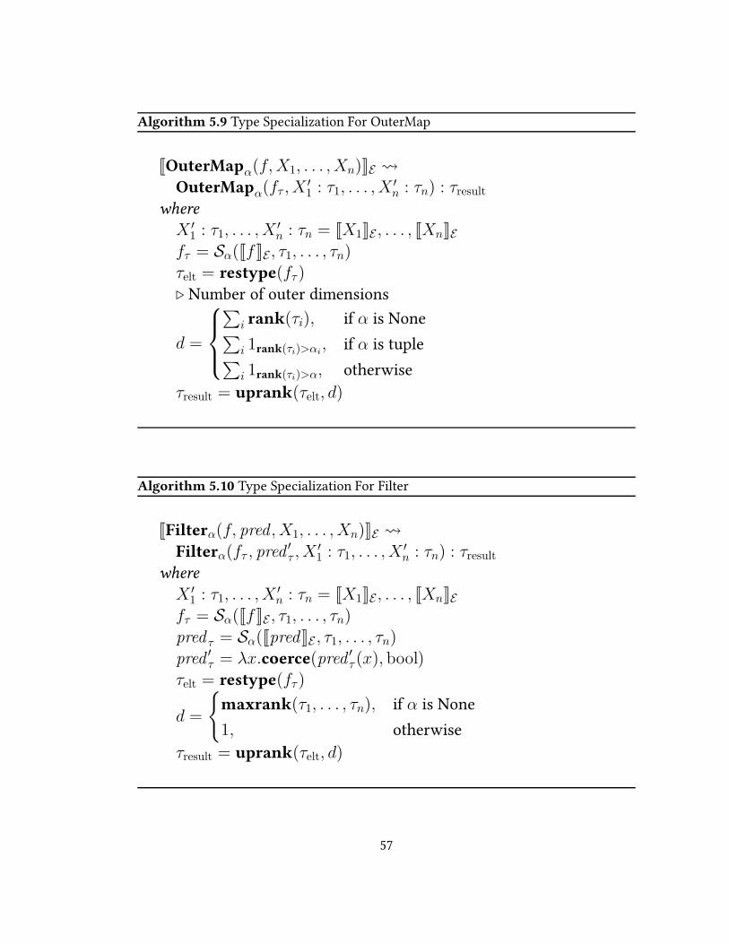
Algorithm 5.9 Type Specialization For OuterMap
JOuterMapα(f,X1, . . . , Xn)KE OuterMapα(fτ , X
′1 : τ1, . . . , X
′n : τn) : τresult
where
X ′1 : τ1, . . . , X
′n : τn = JX1KE , . . . , JXnKE
fτ = Sα(JfKE , τ1, . . . , τn)τelt = restype(fτ)
⊲ Number of outer dimensions
d =
∑
i rank(τi), if α is None∑
i 1rank(τi)>αi, if α is tuple
∑
i 1rank(τi)>α, otherwise
τresult = uprank(τelt, d)
Algorithm 5.10 Type Specialization For Filter
JFilterα(f, pred , X1, . . . , Xn)KE
Filterα(fτ , pred′τ , X
′1 : τ1, . . . , X
′n : τn) : τresult
where
X ′1 : τ1, . . . , X
′n : τn = JX1KE , . . . , JXnKE
fτ = Sα(JfKE , τ1, . . . , τn)
pred τ = Sα(JpredKE , τ1, . . . , τn)pred ′
τ = λx.coerce(pred ′τ (x), bool)
τelt = restype(fτ)
d =
{
maxrank(τ1, . . . , τn), if α is None
1, otherwise
τresult = uprank(τelt, d)
57
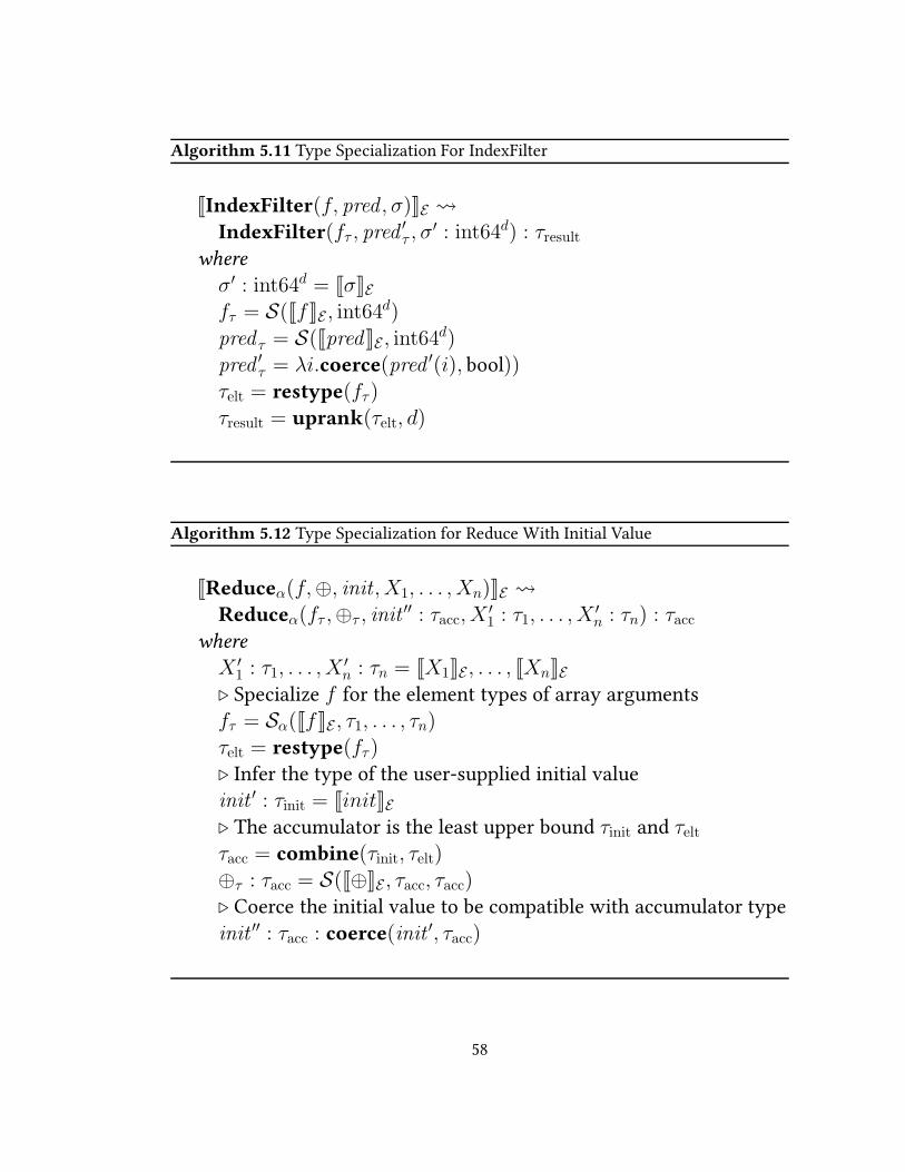
Algorithm 5.11 Type Specialization For IndexFilter
JIndexFilter(f, pred , σ)KE IndexFilter(fτ , pred
′τ , σ
′ : int64d) : τresultwhere
σ′ : int64d = JσKEfτ = S(JfKE , int64
d)
pred τ = S(JpredKE , int64d)
pred ′τ = λi.coerce(pred ′(i), bool))
τelt = restype(fτ)τresult = uprank(τelt, d)
Algorithm 5.12 Type Specialization for Reduce With Initial Value
JReduceα(f,⊕, init, X1, . . . , Xn)KE Reduceα(fτ ,⊕τ , init
′′ : τacc, X′1 : τ1, . . . , X
′n : τn) : τacc
where
X ′1 : τ1, . . . , X
′n : τn = JX1KE , . . . , JXnKE
⊲ Specialize f for the element types of array argumentsfτ = Sα(JfKE , τ1, . . . , τn)
τelt = restype(fτ)⊲ Infer the type of the user-supplied initial valueinit ′ : τinit = JinitKE⊲ The accumulator is the least upper bound τinit and τeltτacc = combine(τinit, τelt)
⊕τ : τacc = S(J⊕KE , τacc, τacc)⊲ Coerce the initial value to be compatible with accumulator typeinit ′′ : τacc : coerce(init
′, τacc)
58
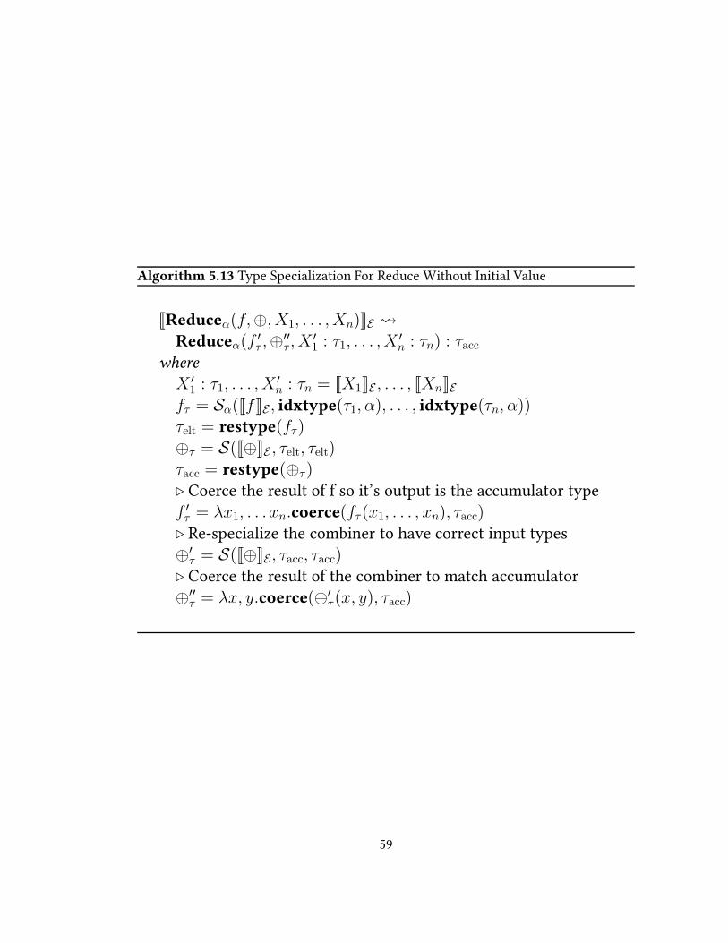
Algorithm 5.13 Type Specialization For Reduce Without Initial Value
JReduceα(f,⊕, X1, . . . , Xn)KE Reduceα(f
′τ ,⊕
′′τ , X
′1 : τ1, . . . , X
′n : τn) : τacc
where
X ′1 : τ1, . . . , X
′n : τn = JX1KE , . . . , JXnKE
fτ = Sα(JfKE , idxtype(τ1, α), . . . , idxtype(τn, α))τelt = restype(fτ)
⊕τ = S(J⊕KE , τelt, τelt)τacc = restype(⊕τ)⊲ Coerce the result of f so it’s output is the accumulator typef ′τ = λx1, . . . xn.coerce(fτ(x1, . . . , xn), τacc)⊲ Re-specialize the combiner to have correct input types⊕′
τ = S(J⊕KE , τacc, τacc)⊲ Coerce the result of the combiner to match accumulator⊕′′
τ = λx, y.coerce(⊕′τ (x, y), τacc)
59
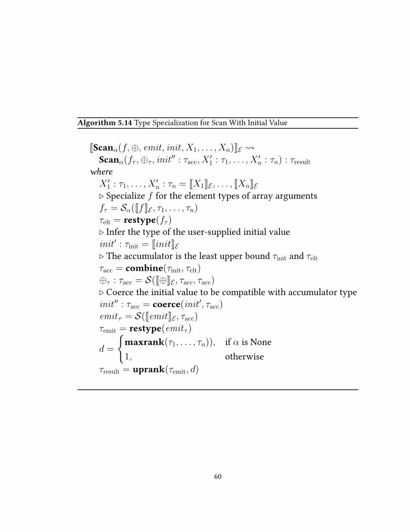
Algorithm 5.14 Type Specialization for Scan With Initial Value
JScanα(f,⊕, emit, init , X1, . . . , Xn)KE
Scanα(fτ ,⊕τ , init′′ : τacc, X
′1 : τ1, . . . , X
′n : τn) : τresult
where
X ′1 : τ1, . . . , X
′n : τn = JX1KE , . . . , JXnKE
⊲ Specialize f for the element types of array argumentsfτ = Sα(JfKE , τ1, . . . , τn)
τelt = restype(fτ)⊲ Infer the type of the user-supplied initial valueinit ′ : τinit = JinitKE⊲ The accumulator is the least upper bound τinit and τeltτacc = combine(τinit, τelt)⊕τ : τacc = S(J⊕KE , τacc, τacc)
⊲ Coerce the initial value to be compatible with accumulator typeinit ′′ : τacc = coerce(init ′, τacc)emit τ = S(JemitKE , τacc)
τemit = restype(emitτ )
d =
{
maxrank(τ1, . . . , τn)), if α is None
1, otherwise
τresult = uprank(τemit, d)
60
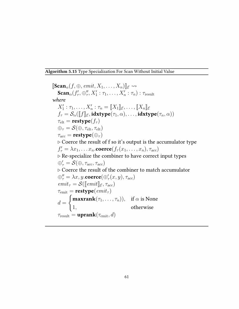
Algorithm 5.15 Type Specialization For Scan Without Initial Value
JScanα(f,⊕, emit, X1, . . . , Xn)KE
Scanα(f′τ ,⊕
′′τ , X
′1 : τ1, . . . , X
′n : τn) : τresult
where
X ′1 : τ1, . . . , X
′n : τn = JX1KE , . . . , JXnKE
fτ = Sα(JfKE , idxtype(τ1, α), . . . , idxtype(τn, α))
τelt = restype(fτ)⊕τ = S(⊕, τelt, τelt)τacc = restype(⊕τ)
⊲ Coerce the result of f so it’s output is the accumulator typef ′τ = λx1, . . . xn.coerce(fτ(x1, . . . , xn), τacc)
⊲ Re-specialize the combiner to have correct input types⊕′
τ = S(⊕, τacc, τacc)
⊲ Coerce the result of the combiner to match accumulator⊕′′
τ = λx, y.coerce(⊕′τ (x, y), τacc)
emit τ = S(JemitKE , τacc)τemit = restype(emitτ )
d =
{
maxrank(τ1, . . . , τn)), if α is None
1, otherwise
τresult = uprank(τemit, d)
61
Chapter 6
Optimizations
Parakeet aggressively optimizes its intermediate representation before attempting to
generate native code. Parakeet’s intermediate representation encodes higher-level se-
mantic properties of a user’s program which are hard to recover when translated to
a backend representation such as C, CUDA, or LLVM. These properties includes the
immutability of tuples, algebraic properties of array operators, and iteration indepen-
dence of parallel constructs such as ParFor. Optimizations which take advantage of
these properties can often have dramatic impact on overall performance. Additionally,
it is important for Parakeet to also perform more traditional compiler optimizations,
in order to better reveal opportunities for high-level restructuring.
The overall structure of Parakeet’s optimization pipeline is:
1. High Level Optimizations. Combine array operators, lower �rst-order operators
such as Range into an explicit Map or IndexMap, lift array operations out of
loops (through Loop Invariant Code Motion), specialize functions on arguments
with known scalar values. None of these optimizations should signi�cantly de-
crease the level of abstraction evident in the code.
62
2. Indexify. Normalize parallel array traversals into a smaller set of constructs by
converting mapping operations such as Map, OuterMap, and IndexMap into
ParFor statements. Similarly, convertReduce into IndexReduce and Scan into
IndexScan. This simpli�es later stages of optimization and allows the backends
to consider a smaller set of parallel primitives.
3. Sequentialize. This optional stage, used only by the sequential C backend, elimi-
nates all parallel constructs and replaces them with sequential loops.
4. Lower Indexing. Transform abstract indexing expressions such as x[i,j] into
explicit dereferencing of a particular memory location determined by the data
pointer and the stride values of the array x.
5. Low-level Optimizations. At this point, allocation should happen explicitly, index-
ing transformed into explicit memory accesses and the code has been reduced to
either a canonical set of parallel operators or parallelism has been removed alto-
gether. Now perform more classical loop optimizations such as a second round
of Loop Invariant Code Motion and Scalar Replacement.
6. Runtime Value Specialization. Even after a function is fully optimized, Parakeet
will attempt to partially evaluate it for “small” inputs, meaning scalars values
equal to 0 or 1, or �elds of structures which contain those values. This can some-
times dramatically improve performance by pruning branches of control �ow or
removing costly indirection.
Parakeet implements this optimization pipeline as a directed acyclic graph of passes,
each of which can be individually deactivated and is associated with metadata such as:
• Is the optimization idempotent or is it unsafe to cache its results?
63
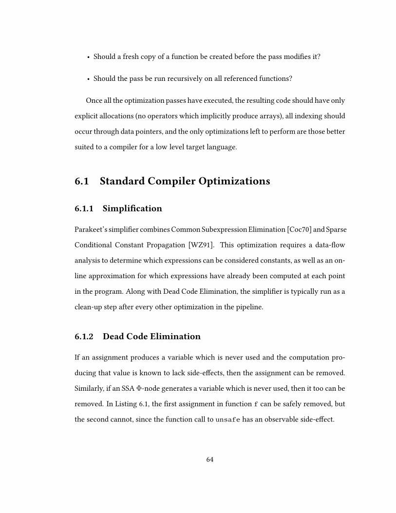
• Should a fresh copy of a function be created before the pass modi�es it?
• Should the pass be run recursively on all referenced functions?
Once all the optimization passes have executed, the resulting code should have only
explicit allocations (no operators which implicitly produce arrays), all indexing should
occur through data pointers, and the only optimizations left to perform are those better
suited to a compiler for a low level target language.
6.1 Standard Compiler Optimizations
6.1.1 Simpli�cation
Parakeet’s simpli�er combines Common Subexpression Elimination [Coc70] and Sparse
Conditional Constant Propagation [WZ91]. This optimization requires a data-�ow
analysis to determine which expressions can be considered constants, as well as an on-
line approximation for which expressions have already been computed at each point
in the program. Along with Dead Code Elimination, the simpli�er is typically run as a
clean-up step after every other optimization in the pipeline.
6.1.2 Dead Code Elimination
If an assignment produces a variable which is never used and the computation pro-
ducing that value is known to lack side-e�ects, then the assignment can be removed.
Similarly, if an SSA Φ-node generates a variable which is never used, then it too can be
removed. In Listing 6.1, the �rst assignment in function f can be safely removed, but
the second cannot, since the function call to unsafe has an observable side-e�ect.
64
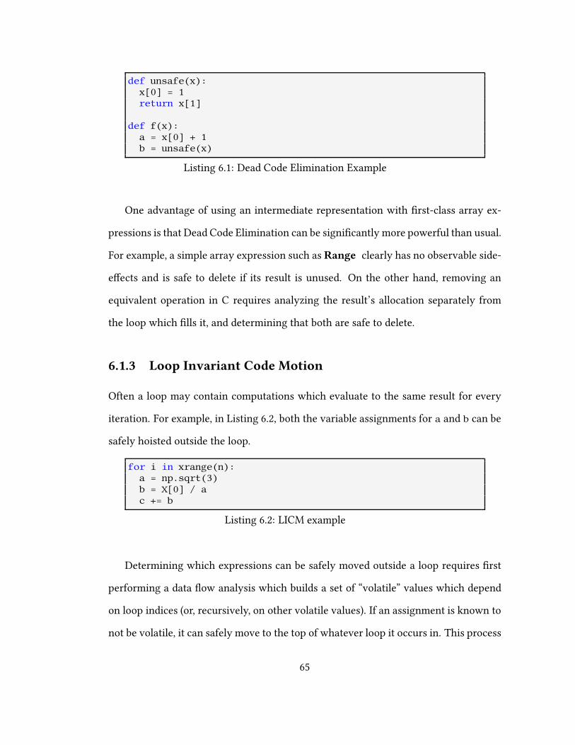
def unsafe(x):x[0] = 1return x[1]
def f(x):a = x[0] + 1b = unsafe(x)
Listing 6.1: Dead Code Elimination Example
One advantage of using an intermediate representation with �rst-class array ex-
pressions is that Dead Code Elimination can be signi�cantly more powerful than usual.
For example, a simple array expression such asRange clearly has no observable side-
e�ects and is safe to delete if its result is unused. On the other hand, removing an
equivalent operation in C requires analyzing the result’s allocation separately from
the loop which �lls it, and determining that both are safe to delete.
6.1.3 Loop Invariant Code Motion
Often a loop may contain computations which evaluate to the same result for every
iteration. For example, in Listing 6.2, both the variable assignments for a and b can be
safely hoisted outside the loop.
for i in xrange(n):a = np.sqrt(3)b = X[0] / ac += b
Listing 6.2: LICM example
Determining which expressions can be safely moved outside a loop requires �rst
performing a data �ow analysis which builds a set of “volatile” values which depend
on loop indices (or, recursively, on other volatile values). If an assignment is known to
not be volatile, it can safely move to the top of whatever loop it occurs in. This process
65
repeats until each expression is either at the top-level scope of a function or considered
volatile.
6.1.4 Scalar Replacement
Scalar replacement [CCK90] is an optimization whereby an array index (e.g. x[i])
which is read from and written to repeatedly within a loop is replaced by a scalar vari-
able. This enhances performance both by allowing that a value to stay in a register
for longer and also enables other optimizations which only work on scalars. This op-
timization requires alias analysis to ensure safety, since two seemingly distinct values
x[i] and y[i] may in fact refer to the same location.
6.2 Fusion
In addition to the more traditional compiler optimizations described above, Parakeet
performs higher-level restructuring “fusion” optimizations that can dramatically im-
prove performance by eliminating array traversals and the creation of intermediate
array values.
In Listing6.3, we show an example of a vector distance function before the applica-
tion of array operator fusion. Notice the repeated traversals byMap operations which
create the array temporaries diff and squared. After the application of fusion, as
shown in Listing 6.4, the two Map operators have been fused into the Reduce oper-
ator, using an input transformation function mapfn. Three array traversals and two
temporaries have been fused into one traversal and no temporaries.
In a loop-oriented imperative language such as Fortran or C, the equivalent to
these optimizations would be loop fusion [Yer66]. Since Parakeet provides higher-
66
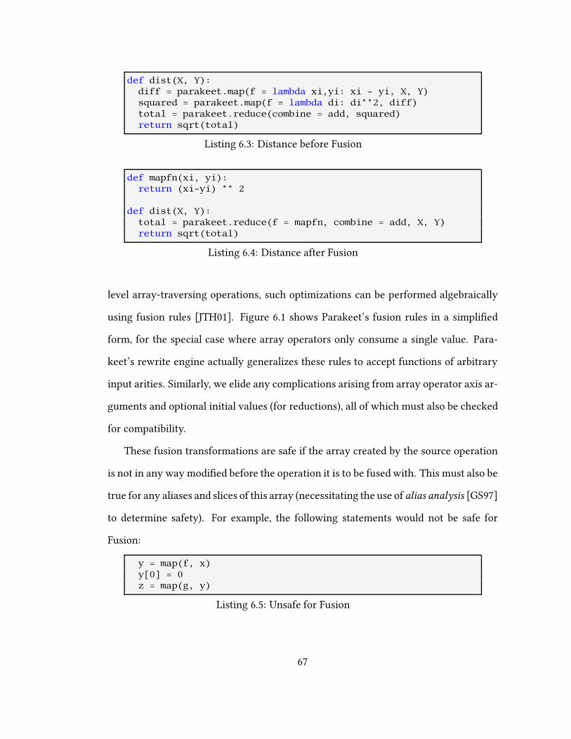
def dist(X, Y):diff = parakeet.map(f = lambda xi,yi: xi - yi, X, Y)squared = parakeet.map(f = lambda di: di**2, diff)total = parakeet.reduce(combine = add, squared)return sqrt(total)
Listing 6.3: Distance before Fusion
def mapfn(xi, yi):return (xi-yi) ** 2
def dist(X, Y):total = parakeet.reduce(f = mapfn, combine = add, X, Y)return sqrt(total)
Listing 6.4: Distance after Fusion
level array-traversing operations, such optimizations can be performed algebraically
using fusion rules [JTH01]. Figure 6.1 shows Parakeet’s fusion rules in a simpli�ed
form, for the special case where array operators only consume a single value. Para-
keet’s rewrite engine actually generalizes these rules to accept functions of arbitrary
input arities. Similarly, we elide any complications arising from array operator axis ar-
guments and optional initial values (for reductions), all of which must also be checked
for compatibility.
These fusion transformations are safe if the array created by the source operation
is not in any way modi�ed before the operation it is to be fused with. This must also be
true for any aliases and slices of this array (necessitating the use of alias analysis [GS97]
to determine safety). For example, the following statements would not be safe for
Fusion:
y = map(f, x)y[0] = 0z = map(g, y)
Listing 6.5: Unsafe for Fusion
67

Parakeet’s fusion optimizations are applied greedily wherever the above safety pre-
requisites are satis�ed. A large body of previous work [AGLP01] has demonstrated that
fusion can be applied more e�ctively when choosing which statements to fuse more
with cost-directed strategies. Still, despite the simplicity of Parakeet’s approach, fusion
has proven both e�ective and absolutely critical for extracting performant compiled
code out of high-level array-oriented user programs. Fusion enables us to boost the
computational density of parallel sections, avoid the generation of unnecessary array
temporaries, and, for the GPU backend, minimize the number of kernel launches.
6.2.1 Nested Fusion
In addition to “vertical” fusion, where values �ow from one statement to another in
the same function, it is also desirable to combined nested operators. For example, if
the parameterizing function of a Map also performs a (nested) Map, then it might be
possible to �atten these two array operators into a single OuterMap. A sketch of the
nested fusion rules is shown in Figure 6.2. The actual implementation, however, is
greatly complicated by the axis parameters, closure arguments, multiple array argu-
ments, and the need to sometimes permute the order arrays to make them compatible
with a particular function.
6.2.2 Horizontal Fusion
The previously discussed fusion optimizations have all involved “vertical” data �ow
from one operator into another. Typically the result of the �rst operator will no longer
be needed after the fusion optimization is applied. In certain cases, it is possible to
take two unrelated computations which traverse the same data or indices and combine
them into a single array operator. This is done by “tupling” the function parameters of
68
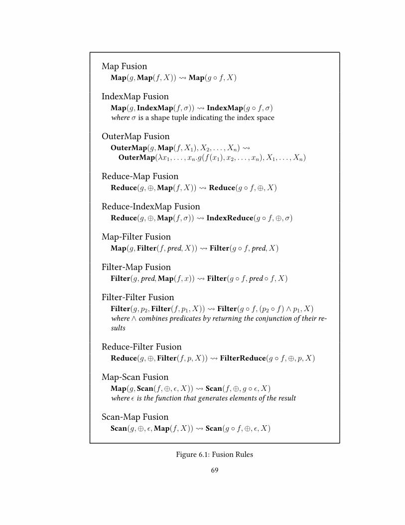
Map FusionMap(g,Map(f,X)) Map(g ◦ f,X)
IndexMap FusionMap(g, IndexMap(f, σ)) IndexMap(g ◦ f, σ)where σ is a shape tuple indicating the index space
OuterMap FusionOuterMap(g,Map(f,X1), X2, . . . , Xn) OuterMap(λx1, . . . , xn.g(f(x1), x2, . . . , xn), X1, . . . , Xn)
Reduce-Map FusionReduce(g,⊕,Map(f,X)) Reduce(g ◦ f,⊕, X)
Reduce-IndexMap FusionReduce(g,⊕,Map(f, σ)) IndexReduce(g ◦ f,⊕, σ)
Map-Filter FusionMap(g, Filter(f, pred, X)) Filter(g ◦ f, pred, X)
Filter-Map FusionFilter(g, pred,Map(f, x)) Filter(g ◦ f, pred ◦ f,X)
Filter-Filter FusionFilter(g, p2, Filter(f, p1, X)) Filter(g ◦ f, (p2 ◦ f) ∧ p1, X)where ∧ combines predicates by returning the conjunction of their re-
sults
Reduce-Filter FusionReduce(g,⊕, Filter(f, p,X)) FilterReduce(g ◦ f,⊕, p,X)
Map-Scan FusionMap(g, Scan(f,⊕, ǫ, X)) Scan(f,⊕, g ◦ ǫ,X)where ǫ is the function that generates elements of the result
Scan-Map FusionScan(g,⊕, ǫ,Map(f,X)) Scan(g ◦ f,⊕, ǫ, X)
Figure 6.1: Fusion Rules
69
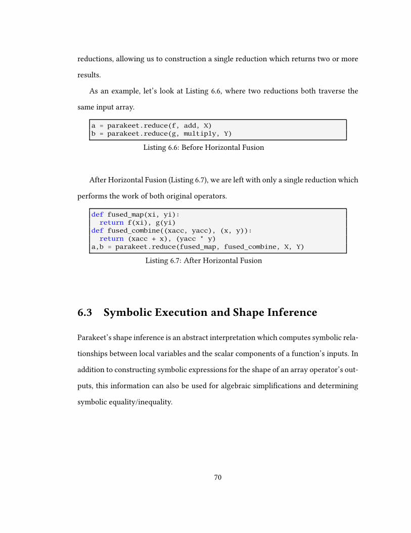
reductions, allowing us to construction a single reduction which returns two or more
results.
As an example, let’s look at Listing 6.6, where two reductions both traverse the
same input array.
a = parakeet.reduce(f, add, X)b = parakeet.reduce(g, multiply, Y)
Listing 6.6: Before Horizontal Fusion
After Horizontal Fusion (Listing 6.7), we are left with only a single reduction which
performs the work of both original operators.
def fused_map(xi, yi):return f(xi), g(yi)
def fused_combine((xacc, yacc), (x, y)):return (xacc + x), (yacc * y)
a,b = parakeet.reduce(fused_map, fused_combine, X, Y)
Listing 6.7: After Horizontal Fusion
6.3 Symbolic Execution and Shape Inference
Parakeet’s shape inference is an abstract interpretation which computes symbolic rela-
tionships between local variables and the scalar components of a function’s inputs. In
addition to constructing symbolic expressions for the shape of an array operator’s out-
puts, this information can also be used for algebraic simpli�cations and determining
symbolic equality/inequality.
70
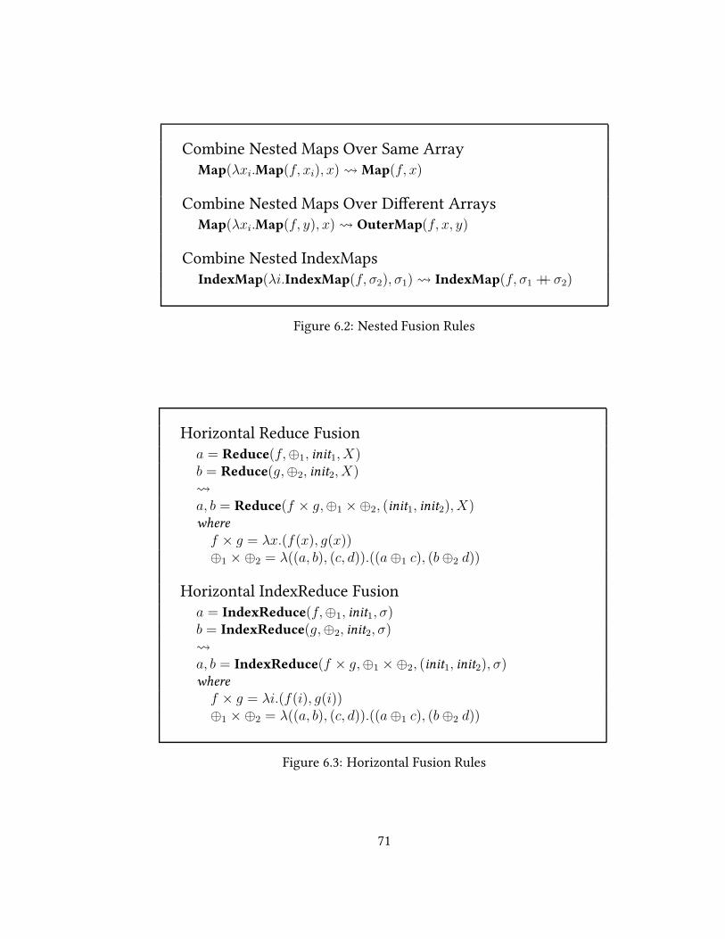
Combine Nested Maps Over Same ArrayMap(λxi.Map(f, xi), x) Map(f, x)
Combine Nested Maps Over Di�erent ArraysMap(λxi.Map(f, y), x) OuterMap(f, x, y)
Combine Nested IndexMapsIndexMap(λi.IndexMap(f, σ2), σ1) IndexMap(f, σ1 ++ σ2)
Figure 6.2: Nested Fusion Rules
Horizontal Reduce Fusiona = Reduce(f,⊕1, init1, X)b = Reduce(g,⊕2, init2, X)
a, b = Reduce(f × g,⊕1 ×⊕2, (init1, init2), X)where
f × g = λx.(f(x), g(x))⊕1 ×⊕2 = λ((a, b), (c, d)).((a⊕1 c), (b⊕2 d))
Horizontal IndexReduce Fusiona = IndexReduce(f,⊕1, init1, σ)b = IndexReduce(g,⊕2, init2, σ)
a, b = IndexReduce(f × g,⊕1 ×⊕2, (init1, init2), σ)where
f × g = λi.(f(i), g(i))⊕1 ×⊕2 = λ((a, b), (c, d)).((a⊕1 c), (b⊕2 d))
Figure 6.3: Horizontal Fusion Rules
71
6.4 Value Specialization
A potential source of ine�ciency for programs which traverse NumPy arrays is that,
by default, all indexing must make use of an auxiliary “strides” array in order to com-
pute the position of elements in the data array. Since indexing is fundamental to all
array reads and writes, it is desirable to eliminate the extra arithmetic and indirection
associated with strided indexing. It is possible to alleviate some of this ine�ciency by
partially evaluating [CD93] a function on the stride values of input arrays. More gen-
erally, it can be bene�cial to perform runtime value specialization [BLR10, CASQP13],
for scalar inputs, elements of tuples, and array strides.
Parakeet performs this optimization by propagating scalar values from the inputs
throughout the source of a function, determining which local variables have statically
determinable values and then constructing a cloned copy of the function with these
variables replaced by constants. Specialized values are propagated recursively through
higher-order array operators, function calls, and ParFor statements. Since partially
evaluating a function on all possible scalar inputs can result in a wasteful process of
never-ending recompilation, Parakeet restricts this optimization to only propagate in-
put values in the set {0, 1, 0.0, 1.0, False,True}, and structures which contain these
values. This optimization can be viewed as analogous to creating singleton type for a
subset of input values as done in type directed partial evaluation [Dan96]
72
Chapter 7
Evaluation
In this section, we will examine the degree to which Parakeet accelerates a variety of
computationally intensive algorithms. The source of each benchmark is given, along
with its performance under the standard Python interpreter CPython, aswell as perfor-
mance under all three of Parakeet’s backends: the single core C backend, the multi-core
OpenMPbackend, and theGPUCUDAbackend. In addition, wemay also comparewith
any easily-accesible Python library functions which implement the same algorithm.
The degree to which Parakeet accelerates code depends most of all on whether that
code spends most of its time in the Python interpreter. In the worst case for Python,
when execution time is dominated by some highly optimized low-level routine, then
Parakeet may in fact run slower than Python. On the other hand, if a large number of
data elements are being inspected within “pure” Python code, then Parakeet may run
the same code several thousand times faster.
A secondary consideration when determining to what degree one should expect a
speed-up from Parakeet is how much parallelism is available. If an algorithm consists
largely of array operations, NumPy library functions, or comprehensions, then Para-
73
keet will be able to extract from all of those data parallel operators. which in term can
be compiled into GPU kernels or multi-core saturating OpenMP declarations.
Lastly, we consider the question of Parakeet’s backends. By default, Parakeet uses
its OpenMP backend. It is possible, on certain examples, to gain a signi�cant perfor-
mance boost from the GPU. In other examples, however, the GPU can be a performance
liability, due to either ine�cient CUDA code generation or the overhead of transferring
data to and from device memory. Furthermore, some algorithms will simply not run
on the GPU at all, particularly those which use more system memory than is available
on the device or which require nested memory allocation within a GPU kernel.
All benchmarks presented here were executed on a machine with 4 Xeon W3520
cores running at 2.67GHz, 12GB of memory, and an NVIDIA GTX 580 video card. The
software used was Ubuntu Linux 12.10, Python 2.7.6, NumPy 1.8.0, CUDA 5.5, and the
development branch of Parakeet 0.25.
7.1 Growcut
Growcut [VK05] is an automata-based image segmentation algorithm. It takes an im-
age and a user-speci�edmask and then repeatedly applies the automata evolution rule
below to derive a �nal segmentation.
Table 7.1 shows the execution times of this Growcut implementation for 500x500 �oat64
image inputs. This benchmark represents a best-case scenario for Parakeet’s speed-up
over Python. In the absence of runtime compilation, all of the computation occurs
inside the Python interpreter, resulting in hopelessly slow performance.
74
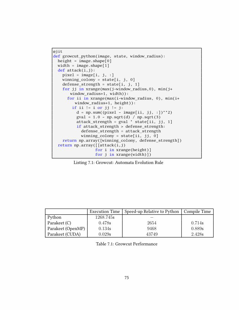
@jitdef growcut_python(image, state, window_radius):
height = image.shape[0]width = image.shape[1]def attack(i,j):
pixel = image[i, j, :]winning_colony = state[i, j, 0]defense_strength = state[i, j, 1]for jj in xrange(max(j-window_radius,0), min(j+
window_radius+1, width)):for ii in xrange(max(i-window_radius, 0), min(i+
window_radius+1, height)):if ii != i or jj != j:
d = np.sum((pixel - image[ii, jj, :])**2)gval = 1.0 - np.sqrt(d) / np.sqrt(3)attack_strength = gval * state[ii, jj, 1]if attack_strength > defense_strength:
defense_strength = attack_strengthwinning_colony = state[ii, jj, 0]
return np.array([winning_colony, defense_strength])return np.array([[attack(i,j)
for i in xrange(height)]for j in xrange(width)])
Listing 7.1: Growcut: Automata Evolution Rule
Execution Time Speed-up Relative to Python Compile TimePython 1268.745s −Parakeet (C) 0.478s 2654 0.714sParakeet (OpenMP) 0.134s 9468 0.889sParakeet (CUDA) 0.029s 43749 2.428s
Table 7.1: Growcut Performance
75

7.2 Matrix Multiplication
Matrix multiplication is one of the most heavily optimized algorithms in the whole of
numerical computing. The one-line Python implementation show in Listing 7.2 cap-
tures the essence of matrix multiplication, unmarred by performance tweaks or op-
timizations. This style of programming, in fact, is ideal for Parakeet since it reveals
parallelizable structure without any potentially confound explicit loops. A well tuned
low-level implementation [WD98, GVDG08], on the other hand can consist of thou-
sands of lines of Fortran, sometimes stitching together machine-generated “codelets”
through auto-tuning.
def matmult(X,Y):return np.array([[np.dot(x,y) for y in Y.T] for x in X])
Listing 7.2: Matrix Multiplication
Shown in Table 7.2 are the execution times for 1200x1200 inputmatriceswith �oat32
element types. The performance under Python is actually surprisingly good, largely
since the dot product operation is being performed by NumPy using an e�cient im-
plementation. For comparison, we also show the performance of a “purer” Python
implementation which de�nes the dot product in terms Python’s builtin sum function.
We also compare with the performance of a highly tuned multi-core CPU library, AT-
LAS [WD98] and its GPU equivalent, CUBLAS [BCI+08].
Unsurprisingly, ATLAS’s tightly optimized multi-core matrix multiplication algo-
rithm signi�cantly outperform Parakeet’s C and OpenMP backends. Similarly, the
CUBLAS library outperforms Parakeet’s naively generated CUDA code. A signi�cant
factor in this performance gap is Parakeet’s lack of cache tiling [WL91]. We have previ-
ously investigated tiled data parallel operators [HRS13] which group array inputs into
76
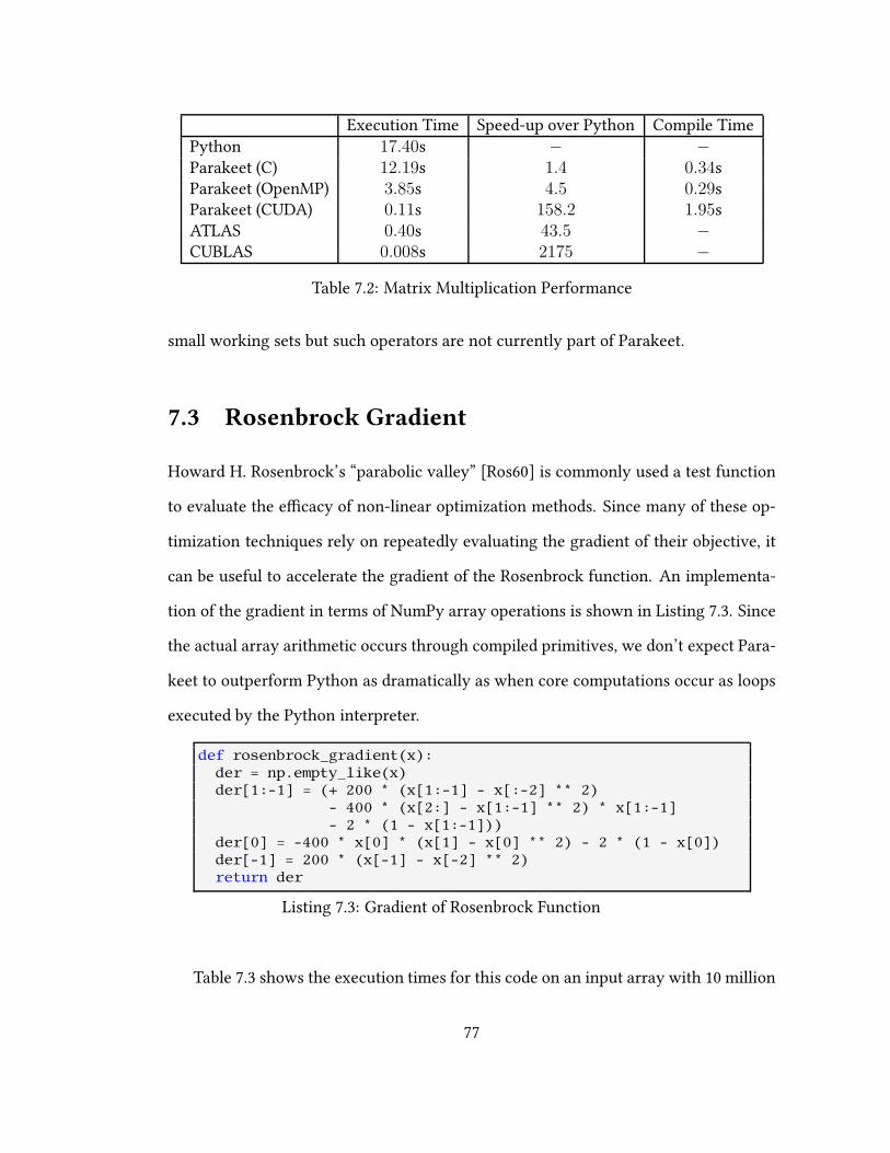
Execution Time Speed-up over Python Compile TimePython 17.40s − −Parakeet (C) 12.19s 1.4 0.34sParakeet (OpenMP) 3.85s 4.5 0.29sParakeet (CUDA) 0.11s 158.2 1.95sATLAS 0.40s 43.5 −CUBLAS 0.008s 2175 −
Table 7.2: Matrix Multiplication Performance
small working sets but such operators are not currently part of Parakeet.
7.3 Rosenbrock Gradient
Howard H. Rosenbrock’s “parabolic valley” [Ros60] is commonly used a test function
to evaluate the e�cacy of non-linear optimization methods. Since many of these op-
timization techniques rely on repeatedly evaluating the gradient of their objective, it
can be useful to accelerate the gradient of the Rosenbrock function. An implementa-
tion of the gradient in terms of NumPy array operations is shown in Listing 7.3. Since
the actual array arithmetic occurs through compiled primitives, we don’t expect Para-
keet to outperform Python as dramatically as when core computations occur as loops
executed by the Python interpreter.
def rosenbrock_gradient(x):der = np.empty_like(x)der[1:-1] = (+ 200 * (x[1:-1] - x[:-2] ** 2)
- 400 * (x[2:] - x[1:-1] ** 2) * x[1:-1]- 2 * (1 - x[1:-1]))
der[0] = -400 * x[0] * (x[1] - x[0] ** 2) - 2 * (1 - x[0])der[-1] = 200 * (x[-1] - x[-2] ** 2)return der
Listing 7.3: Gradient of Rosenbrock Function
Table 7.3 shows the execution times for this code on an input array with 10 million
77
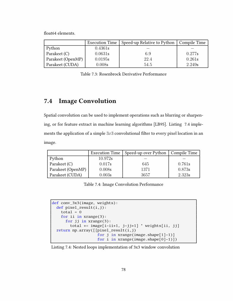
�oat64 elements.
Execution Time Speed-up Relative to Python Compile TimePython 0.4361s − −Parakeet (C) 0.0631s 6.9 0.277sParakeet (OpenMP) 0.0195s 22.4 0.261sParakeet (CUDA) 0.008s 54.5 2.249s
Table 7.3: Rosenbrock Derivative Performance
7.4 Image Convolution
Spatial convolution can be used to implement operations such as blurring or sharpen-
ing, or for feature extract in machine learning algorithms [LB95]. Listing 7.4 imple-
ments the application of a simple 3x3 convolutional �lter to every pixel location in an
image.
Execution Time Speed-up over Python Compile TimePython 10.972s − −Parakeet (C) 0.017s 645 0.761sParakeet (OpenMP) 0.008s 1371 0.873sParakeet (CUDA) 0.003s 3657 2.323s
Table 7.4: Image Convolution Performance
def conv_3x3(image, weights):def pixel_result(i,j):
total = 0for ii in xrange(3):
for jj in xrange(3):total += image[i-ii+1, j-jj+1] * weights[ii, jj]
return np.array([[pixel_result(i,j)for j in xrange(image.shape[1]-1)]for i in xrange(image.shape[0]-1)])
Listing 7.4: Nested loops implementation of 3x3 window convolution
78
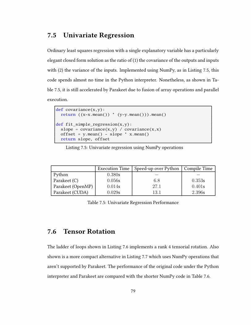
7.5 Univariate Regression
Ordinary least squares regression with a single explanatory variable has a particularly
elegant closed form solution as the ratio of (1) the covariance of the outputs and inputs
with (2) the variance of the inputs. Implemented using NumPy, as in Listing 7.5, this
code spends almost no time in the Python interpreter. Nonetheless, as shown in Ta-
ble 7.5, it is still accelerated by Parakeet due to fusion of array operations and parallel
execution.
def covariance(x,y):return ((x-x.mean()) * (y-y.mean())).mean()
def fit_simple_regression(x,y):slope = covariance(x,y) / covariance(x,x)offset = y.mean() - slope * x.mean()return slope, offset
Listing 7.5: Univariate regression using NumPy operations
Execution Time Speed-up over Python Compile TimePython 0.380s − −Parakeet (C) 0.056s 6.8 0.353sParakeet (OpenMP) 0.014s 27.1 0.401sParakeet (CUDA) 0.029s 13.1 2.396s
Table 7.5: Univariate Regression Performance
7.6 Tensor Rotation
The ladder of loops shown in Listing 7.6 implements a rank 4 tensorial rotation. Also
shown is a more compact alternative in Listing 7.7 which uses NumPy operations that
aren’t supported by Parakeet. The performance of the original code under the Python
interpreter and Parakeet are compared with the shorter NumPy code in Table 7.6.
79
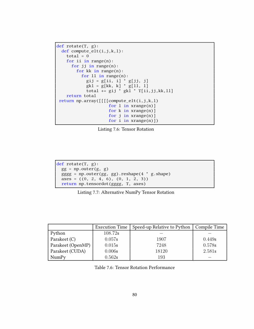
def rotate(T, g):def compute_elt(i,j,k,l):
total = 0for ii in range(n):
for jj in range(n):for kk in range(n):
for ll in range(n):gij = g[ii, i] * g[jj, j]gkl = g[kk, k] * g[ll, l]total += gij * gkl * T[ii,jj,kk,ll]
return totalreturn np.array([[[[compute_elt(i,j,k,l)
for l in xrange(n)]for k in xrange(n)]for j in xrange(n)]for i in xrange(n)])
Listing 7.6: Tensor Rotation
def rotate(T, g):gg = np.outer(g, g)gggg = np.outer(gg, gg).reshape(4 * g.shape)axes = ((0, 2, 4, 6), (0, 1, 2, 3))return np.tensordot(gggg, T, axes)
Listing 7.7: Alternative NumPy Tensor Rotation
Execution Time Speed-up Relative to Python Compile TimePython 108.72s − −Parakeet (C) 0.057s 1907 0.449sParakeet (OpenMP) 0.015s 7248 0.578sParakeet (CUDA) 0.006s 18120 2.581sNumPy 0.562s 193 −
Table 7.6: Tensor Rotation Performance
80
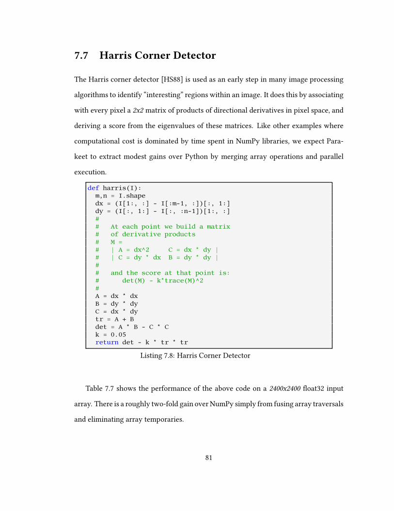
7.7 Harris Corner Detector
The Harris corner detector [HS88] is used as an early step in many image processing
algorithms to identify “interesting” regions within an image. It does this by associating
with every pixel a 2x2 matrix of products of directional derivatives in pixel space, and
deriving a score from the eigenvalues of these matrices. Like other examples where
computational cost is dominated by time spent in NumPy libraries, we expect Para-
keet to extract modest gains over Python by merging array operations and parallel
execution.
def harris(I):m,n = I.shapedx = (I[1:, :] - I[:m-1, :])[:, 1:]dy = (I[:, 1:] - I[:, :n-1])[1:, :]## At each point we build a matrix# of derivative products# M =# | A = dx^2 C = dx * dy |# | C = dy * dx B = dy * dy |## and the score at that point is:# det(M) - k*trace(M)^2#A = dx * dxB = dy * dyC = dx * dytr = A + Bdet = A * B - C * Ck = 0.05return det - k * tr * tr
Listing 7.8: Harris Corner Detector
Table 7.7 shows the performance of the above code on a 2400x2400 �oat32 input
array. There is a roughly two-fold gain over NumPy simply from fusing array traversals
and eliminating array temporaries.
81
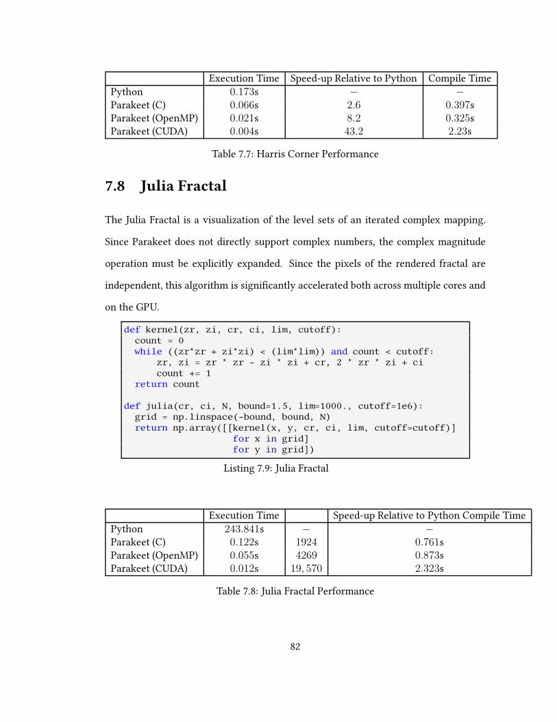
Execution Time Speed-up Relative to Python Compile TimePython 0.173s − −Parakeet (C) 0.066s 2.6 0.397sParakeet (OpenMP) 0.021s 8.2 0.325sParakeet (CUDA) 0.004s 43.2 2.23s
Table 7.7: Harris Corner Performance
7.8 Julia Fractal
The Julia Fractal is a visualization of the level sets of an iterated complex mapping.
Since Parakeet does not directly support complex numbers, the complex magnitude
operation must be explicitly expanded. Since the pixels of the rendered fractal are
independent, this algorithm is signi�cantly accelerated both across multiple cores and
on the GPU.
def kernel(zr, zi, cr, ci, lim, cutoff):count = 0while ((zr*zr + zi*zi) < (lim*lim)) and count < cutoff:
zr, zi = zr * zr - zi * zi + cr, 2 * zr * zi + cicount += 1
return count
def julia(cr, ci, N, bound=1.5, lim=1000., cutoff=1e6):grid = np.linspace(-bound, bound, N)return np.array([[kernel(x, y, cr, ci, lim, cutoff=cutoff)]
for x in grid]for y in grid])
Listing 7.9: Julia Fractal
Execution Time Speed-up Relative to Python Compile TimePython 243.841s − −Parakeet (C) 0.122s 1924 0.761sParakeet (OpenMP) 0.055s 4269 0.873sParakeet (CUDA) 0.012s 19, 570 2.323s
Table 7.8: Julia Fractal Performance
82
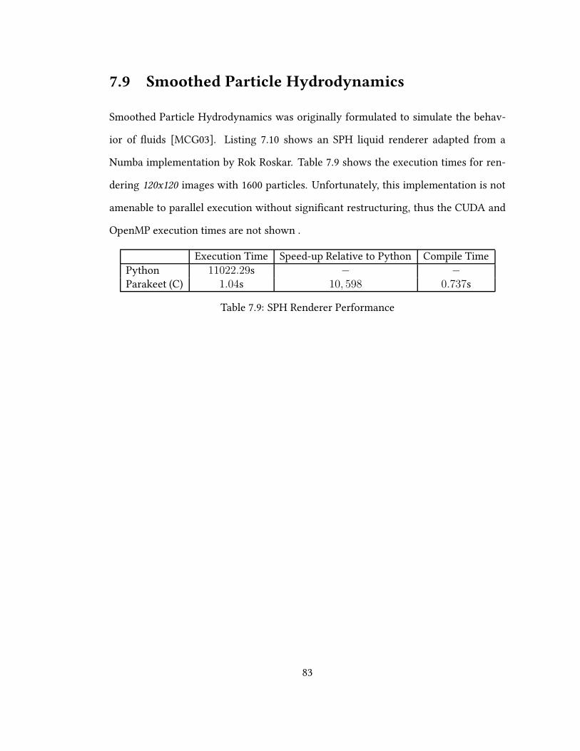
7.9 Smoothed Particle Hydrodynamics
Smoothed Particle Hydrodynamics was originally formulated to simulate the behav-
ior of �uids [MCG03]. Listing 7.10 shows an SPH liquid renderer adapted from a
Numba implementation by Rok Roskar. Table 7.9 shows the execution times for ren-
dering 120x120 images with 1600 particles. Unfortunately, this implementation is not
amenable to parallel execution without signi�cant restructuring, thus the CUDA and
OpenMP execution times are not shown .
Execution Time Speed-up Relative to Python Compile TimePython 11022.29s − −Parakeet (C) 1.04s 10, 598 0.737s
Table 7.9: SPH Renderer Performance
83
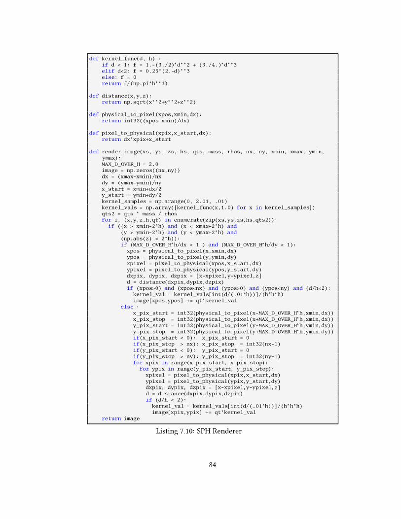
def kernel_func(d, h) :if d < 1: f = 1.-(3./2)*d**2 + (3./4.)*d**3elif d<2: f = 0.25*(2.-d)**3else: f = 0return f/(np.pi*h**3)
def distance(x,y,z):return np.sqrt(x**2+y**2+z**2)
def physical_to_pixel(xpos,xmin,dx):return int32((xpos-xmin)/dx)
def pixel_to_physical(xpix,x_start,dx):return dx*xpix+x_start
def render_image(xs, ys, zs, hs, qts, mass, rhos, nx, ny, xmin, xmax, ymin,ymax):MAX_D_OVER_H = 2.0image = np.zeros((nx,ny))dx = (xmax-xmin)/nxdy = (ymax-ymin)/nyx_start = xmin+dx/2y_start = ymin+dy/2kernel_samples = np.arange(0, 2.01, .01)kernel_vals = np.array([kernel_func(x,1.0) for x in kernel_samples])qts2 = qts * mass / rhosfor i, (x,y,z,h,qt) in enumerate(zip(xs,ys,zs,hs,qts2)):
if ((x > xmin-2*h) and (x < xmax+2*h) and(y > ymin-2*h) and (y < ymax+2*h) and(np.abs(z) < 2*h)):if (MAX_D_OVER_H*h/dx < 1 ) and (MAX_D_OVER_H*h/dy < 1):
xpos = physical_to_pixel(x,xmin,dx)ypos = physical_to_pixel(y,ymin,dy)xpixel = pixel_to_physical(xpos,x_start,dx)ypixel = pixel_to_physical(ypos,y_start,dy)dxpix, dypix, dzpix = [x-xpixel,y-ypixel,z]d = distance(dxpix,dypix,dzpix)if (xpos>0) and (xpos<nx) and (ypos>0) and (ypos<ny) and (d/h<2):
kernel_val = kernel_vals[int(d/(.01*h))]/(h*h*h)image[xpos,ypos] += qt*kernel_val
else :x_pix_start = int32(physical_to_pixel(x-MAX_D_OVER_H*h,xmin,dx))x_pix_stop = int32(physical_to_pixel(x+MAX_D_OVER_H*h,xmin,dx))y_pix_start = int32(physical_to_pixel(y-MAX_D_OVER_H*h,ymin,dy))y_pix_stop = int32(physical_to_pixel(y+MAX_D_OVER_H*h,ymin,dy))if(x_pix_start < 0): x_pix_start = 0if(x_pix_stop > nx): x_pix_stop = int32(nx-1)if(y_pix_start < 0): y_pix_start = 0if(y_pix_stop > ny): y_pix_stop = int32(ny-1)for xpix in range(x_pix_start, x_pix_stop):
for ypix in range(y_pix_start, y_pix_stop):xpixel = pixel_to_physical(xpix,x_start,dx)ypixel = pixel_to_physical(ypix,y_start,dy)dxpix, dypix, dzpix = [x-xpixel,y-ypixel,z]d = distance(dxpix,dypix,dzpix)if (d/h < 2):
kernel_val = kernel_vals[int(d/(.01*h))]/(h*h*h)image[xpix,ypix] += qt*kernel_val
return image
Listing 7.10: SPH Renderer
84

Chapter 8
Conclusion
This thesis set out to save numerically-inclined programmers from having to write in
low-level languages in order to speed up their programs. The existing Parakeet library
isn’t the �nal word in this endeavor but rather a guidepost toward the right direction.
We have demonstrated that compact high-level descriptions of numerical algorithms
can be successfully compiled into e�cient code which runs in parallel across multiple
cores or on a GPU. Furthermore, we have shown the central role played by higher order
data parallel array operators in attaining this goal. The basic contours of Parakeet’s
design, its variety of data parallel operators, typed intermediate representation, and
restructuring optimizations, should be transferrable to other languages beyond Python.
There are several directions along which Parakeet can (and should) be extended:
• Graph-Based Control Flow Representations. While the current structured
SSA representation was useful for quickly prototyping analyses and optimiza-
tions, it prevents the implementation of idiomatic control �ow constructs. To
support a broader subset of Python, it is important to migrate Parakeet to a
proper control �ow graph and reimplement all of Parakeet’s data �ow analyses
85

to work with this more �exible representation.
• StructuredArray Elements. Parakeet is currently limited to arrays with scalar
elements, which forces it to reject many NumPy programs which use structured
element types. Parakeet should be able to support not only to support these
kinds of arrays, but to e�ciently reorganize their layout via the standard array-
of-structs to struct-of-arrays transformation.
• User-de�ned Objects. Parakeet cannot currently accelerate methods or use
any sort of user-de�ned objects within its intermediate representation. It should
be possible to partially lift these restrictions by treating objects as immutable
records. A more ambitious attempt to fully support the semantics of Python
objects would require a dramatic rethinking both of Parakeet’s type system and
of its assumptions regarding mutability.
• Data-Dependent Broadcasting. Parakeet implements a restriction of NumPy’s
notion of broadcasting. When two values of di�ering ranks are combined (a ma-
trix and scalar, or a matrix and vector), Parakeet inserts an explicit Map oper-
ation to implement the logic of broadcasting. However, Parakeet is not able to
support broadcasting which occurs due to unit dimensions, such adding a 200x1
matrix with a 1x300 matrix to get a 200x300 result. It should be possible to add
dynamic broadcasting as part of the semantics of higher order array operators,
though this may incur some additional overhead.
• Full NumPy Support. If Parakeet were expanded and improvement in all the
waysmentioned above, then it might be possible to fully wrap the NumPy library
and support any unmodi�ed code which restricts itself to array operations.
86
• Shorter Compile Times for GPU Backend. Despite the impressive perfor-
mance attained by the CUDA backend, it is still not ready to be used as the de-
fault compilation pathway in Parakeet. One of the major reasons for this are the
extremely long compile times incurred through the use of NVIDIA’s nvcc com-
piler. In the future, it should be possible to dramatically decrease these compile
times by targeting the GPU pseudo-assembly language PTX directly, bypassing
the central overhead of CUDA compilation.
• Better utilizations of sharedmemory onGPU. The current compilation tem-
plate for GPU kernels in Parakeet is very naive and makes no use of the GPU’s
software managed cache (called sharedmemory). Utilization of this cache is often
critical for attaining good performance on the GPU and thus it is strongly desir-
able for compiled code to do so. One possible avenue by which at least some pro-
grams can bene�t from shared memory is to identify nested reductions within a
parallel operator and to have a distinct compilation template for this case which
pre-loads inputs into shared memory and then performs a “tree-structured” re-
duction.
• Heterogeneous Execution. The easiest way to facilitate the use of multiple
GPUs, along with multi-core CPUs, is to identify bulk operations which can be
concurrently executed and to assign each operation to a particular device. It may
also be possible to achieve a more �ne-grained heterogeneity, wherein a single
operation is split between GPU(s) and CPU cores. This would require a more
nuanced notion of where data lives, since portions of an array could be split
across multiple memory spaces.
Despite its limitations, however, Parakeet already supports a wide range of numer-
87
ical Python programs and enables their e�cient execution on parallel hardware. The
future of scienti�c programming lies with high-level collection-oriented languages.
Runtime compilation techniques, like those found in Parakeet, will be essential for
eliminating the cost of abstraction and freeing scienti�c programmers to simply write
what they mean.
88

89
89

Bibliography
[Abr70] Philip Samuel Abrams. An APL machine. PhD thesis, Stanford, CA, USA,
1970.
[AGLP01] Marco Aldinucci, Sergei Gorlatch, Christian Lengauer, and Susanna Pela-
gatti. Towards parallel programming by transformation: the FAN skeleton
framework. Parallel Algorithms Appl., 16(2-3):87–121, 2001.
[All70] Frances E. Allen. Control �ow analysis. In Proceedings of a Symposium on
Compiler Optimization, pages 1–19, New York, NY, USA, 1970. ACM.
[AS79] WalidAbdul-KarimAbu-Sufah. Improving the performance of virtual mem-
ory computers. PhD thesis, Champaign, IL, USA, 1979.
[Ayc03] J. Aycock. A brief history of just-in-time. ACMComputing Surveys (CSUR),
35(2):97–113, 2003.
[BBB+57] John W Backus, Robert J Beeber, Sheldon Best, Richard Goldberg,
L Mitchell Haibt, Harlan L Herrick, Robert A Nelson, David Sayre, Pe-
ter B Sheridan, H Stern, et al. The FORTRAN automatic coding system. In
Papers presented at the February 26-28, 1957, western joint computer confer-
ence: Techniques for reliability, pages 188–198. ACM, 1957.
90
[BBB+10] James Bergstra, Olivier Breuleux, Frédéric Bastien, Pascal Lamblin, Raz-
van Pascanu, Guillaume Desjardins, Joseph Turian, David Warde-Farley,
and Yoshua Bengio. Theano: a cpu and gpu math expression compiler.
In Proceedings of the Python for Scienti�c Computing Conference (SciPy),
volume 4, 2010.
[BBC+11] Stefan Behnel, Robert Bradshaw, Craig Citro, Lisandro Dalcin, Dag Sverre
Seljebotn, and Kurt Smith. Cython: The best of both worlds. Computing
in Science & Engineering, 13(2):31–39, 2011.
[BBH+63] David W Barron, John N Buxton, DF Hartley, E Nixon, and Christopher
Strachey. The main features of cpl. The Computer Journal, 6(2):134–143,
1963.
[BCF+93] Zeki Bozkus, Alok Choudhary, Geo�rey Fox, Tomasz Haupt, and Sanjay
Ranka. Fortran 90d/hpf compiler for distributed memory mimd comput-
ers: Design, implementation, and performance results. In Proceedings of
the 1993 ACM/IEEE conference on Supercomputing, pages 351–360. ACM,
1993.
[BCH+94] Guy E. Blelloch, S. Chatterjee, J. C. Hardwick, J. Sipelstein, and M. Zagha.
Implementation of a portable nested data-parallel language. Journal of
Parallel and Distributed Computing, 21(1):4–14, Apr. 1994.
[BCI+08] Sergio Barrachina, Maribel Castillo, Francisco D Igual, Rafael Mayo, and
Enrique S Quintana-Orti. Evaluation and tuning of the level 3 cublas for
graphics processors. In Parallel and Distributed Processing, 2008. IPDPS
2008. IEEE International Symposium on, pages 1–8. IEEE, 2008.
91
[Ber97] Robert Bernecky. Apex: The apl parallel executor. 1997.
[Blo03] Joshua Bloom. Python as super glue for the modern scienti�c work-
�ow. http://www.youtube.com/watch?v=mLuIB8aW2KA,
2003. Accessed: 2013-12-03.
[BLR10] Carl Friedrich Bolz, Michael Leuschel, and Armin Rigo. Towards just-in-
time partial evaluation of prolog. In Logic-Based Program Synthesis and
Transformation, pages 158–172. Springer, 2010.
[BM94] Marc M. Brandis and Hanspeter Mössenböck. Single-pass generation of
static single-assignment form for structured languages. ACM Trans. Pro-
gram. Lang. Syst., 16(6):1684–1698, November 1994.
[Bor08] Je�rey A. Borror. Q For Mortals: A Tutorial In Q Programming. CreateS-
pace, 2008.
[BTCGS91] Val Breazu-Tannen, Thierry Coquand, Carl A Gunter, and Andre Scedrov.
Inheritance as implicit coercion. Information and computation, 93(1):172–
221, 1991.
[Bud83] Timothy A Budd. An apl compiler for the unix timesharing system. In
ACM SIGAPL APL Quote Quad, volume 13, pages 205–209. ACM, 1983.
[Bud84] Timothy A. Budd. An APL compiler for a vector processor. ACM Trans.
Program. Lang. Syst., 6(3):297–313, July 1984.
[CASQP13] Igor Costa, Péricles Alves, Henrique Nazaré Santos, and Fernando Magno
Quintao Pereira. Just-in-time value specialization. In Code Generation and
92
Optimization (CGO), 2013 IEEE/ACM International Symposium on, pages
1–11. IEEE, 2013.
[CCK90] David Callahan, Steve Carr, and Ken Kennedy. Improving register alloca-
tion for subscripted variables. In Proceedings of the ACM SIGPLAN 1990
Conference on Programming Language Design and Implementation, PLDI
’90, pages 53–65, New York, NY, USA, 1990. ACM.
[CD93] Charles Consel and Olivier Danvy. Tutorial notes on partial evaluation.
In Proceedings of the 20th ACM SIGPLAN-SIGACT symposium on Principles
of programming languages, pages 493–501. ACM, 1993.
[CF90] DavidCann and John Feo. Sisal versus fortran: A comparison using the liv-
ermore loops. In Supercomputing’90. Proceedings of, pages 626–636. IEEE,
1990.
[CFR+89] Ron Cytron, Jeanne Ferrante, Barry K Rosen, Mark NWegman, and F Ken-
neth Zadeck. An e�cient method of computing static single assignment
form. In Proceedings of the 16th ACM SIGPLAN-SIGACT symposium on
Principles of programming languages, pages 25–35. ACM, 1989.
[CFR+91] Ron Cytron, Jeanne Ferrante, Barry K. Rosen, Mark N. Wegman, and
F. Kenneth Zadeck. E�ciently computing static single assignment form
and the control dependence graph. ACM Trans. Program. Lang. Syst.,
13:451–490, October 1991.
[CGK11] Bryan Catanzaro, Michael Garland, and Kurt Keutzer. Copperhead: Com-
piling an embedded data parallel language. In Proceedings of the 16th ACM
93
Symposium on Principles and Practice of Parallel Programming (PPoPP),
pages 47–56, 2011.
[CH] David Cooke and Timothy Hochberg. Numexpr. fast evaluation of array
expressions by using a vector-based virtual machine.
[Chi86] Wai-MeeChing. Program analysis and code generation in an apl/370 com-
piler. IBM Journal of Research and Development, 30(6):594–602, 1986.
[Coc70] John Cocke. Global common subexpression elimination. In Proceedings of
a Symposium on Compiler Optimization, pages 20–24, New York, NY, USA,
1970. ACM.
[Con] Continuum Analytics. Numba. http://numba.pydata.org.
[CP79] S. Cohen and S. Piper. Speakeasy iii reference manual. Speakeasy Com-
puting Corp., Chicago, Ill., 1979.
[Dan96] Olivier Danvy. Pragmatics of type-directed partial evaluation. Springer,
1996.
[DM98] Leonardo Dagum and Ramesh Menon. Openmp: an industry standard api
for shared-memory programming. Computational Science & Engineering,
IEEE, 5(1):46–55, 1998.
[FBB06] A. Fitzpatrick, S. Berkovich, and S. Berkovich. Mesm and the beginning of
the computer era in the soviet union. Annals of the History of Computing,
IEEE, 28(3):4–16, 2006.
94
[FJ05] Matteo Frigo and Steven G. Johnson. The design and implementation of
FFTW3. Proceedings of the IEEE, 93:216–231, 2005. Special Issue on "Pro-
gram Generation, Optimization, and Adaptation".
[GBA13] Serge Guelton, Pierrick Brunet, and Mehdi Amini. Compiling Python
modules to native parallel modules using Pythran and OpenMP annota-
tions. In Python for High Performance and Scienti�c Computing 2013, 2013.
[GG46] Herman H Goldstine and Adele Goldstine. The electronic numerical inte-
grator and computer (eniac). Mathematical Tables and Other Aids to Com-
putation, 2(15):97–110, 1946.
[Gre07] P. Green�eld. Reaching for the stars with python. Computing in Science
Engineering, 9(3):38–40, 2007.
[GS97] K Gopinath and R Seshadri. Alias analysis for fortran90 array slices. In
Parallel Processing Symposium, 1997. Proceedings., 11th International, pages
628–632. IEEE, 1997.
[GVDG08] Kazushige Goto and Robert Van De Geijn. High-performance implemen-
tation of the level-3 BLAS. ACM Transactions on Mathematical Software,
35(1):4:1–4:14, July 2008.
[HI98] Roger KW Hui and Kenneth E Iverson. J: Dictionary. Iverson Software,
1998.
[HRS13] Eric Hielscher, Alex Rubinsteyn, andDennis Shasha. Locality optimization
for data parallel programs. arXiv preprint arXiv:1304.1835, 2013.
95
[HS88] Chris Harris and Mike Stephens. A combined corner and edge detector.
In Alvey vision conference, volume 15, page 50. Manchester, UK, 1988.
[Hun07] John D Hunter. Matplotlib: A 2d graphics environment. Computing in
Science & Engineering, pages 90–95, 2007.
[IG96] Ross Ihaka and Robert Gentleman. R: A language for data analysis and
graphics. Journal of computational and graphical statistics, 5(3):299–314,
1996.
[Ive62] Kenneth E. Iverson. A programming language. In Proceedings of the May
1-3, 1962, spring joint computer conference, AIEE-IRE ’62 (Spring), pages
345–351, 1962.
[JGM86] MichaelA. Jenkins, Janice I. Glasgow, andCarl DMcCrosky. Programming
styles in nial. Software, IEEE, 3(1):46–55, 1986.
[Joh85] Thomas Johnsson. Lambda lifting: Transforming programs to recursive
equations. In Functional programming languages and computer architec-
ture, pages 190–203. Springer, 1985.
[JOP01] Eric Jones, Travis Oliphant, and Pearu Peterson. Scipy: Open source sci-
enti�c tools for python. http://www. scipy. org/, 2001.
[JTH01] Simon Peyton Jones, Andrew Tolmach, and Tony Hoare. Playing by the
rules: rewriting as a practical optimisation technique in GHC. In Proceed-
ings of the 2004 Haskell Workshop, 2001.
[Kin12] Volodymyr Kindratenko. Scienti�c computing with gpus. Computing in
Science & Engineering, 14(3):8–9, 2012.
96
[KM93] Ken Kennedy and Kathryn S. Mckinley. Typed fusion with applications to
parallel and sequential code generation. Technical report, 1993.
[KRE88] Brian W Kernighan, Dennis M Ritchie, and Per Ejeklint. The C program-
ming language, volume 2. prentice-Hall Englewood Cli�s, 1988.
[KSH12] Alex Krizhevsky, Ilya Sutskever, and Geo�Hinton. Imagenet classi�cation
with deep convolutional neural networks. In Advances in Neural Informa-
tion Processing Systems 25, pages 1106–1114, 2012.
[KY13] Matthew G Knepley and David A Yuen. Why do scientists and engineers
need gpu’s today? In GPU Solutions to Multi-scale Problems in Science and
Engineering, pages 3–11. Springer, 2013.
[LB95] Yann LeCun and Yoshua Bengio. Convolutional networks for images,
speech, and time series. The handbook of brain theory and neural networks,
3361, 1995.
[LS94] Calvin Lin and Lawrence Snyder. Zpl: An array sublanguage. In Languages
and Compilers for Parallel Computing, pages 96–114. Springer, 1994.
[MAT10] MATLAB. version 7.10.0 (R2010a). The MathWorks Inc., Natick, Mas-
sachusetts, 2010.
[McC61] John McCarthy. A basis for a mathematical theory of computation, pre-
liminary report. In Papers presented at the May 9-11, 1961, western joint
IRE-AIEE-ACM computer conference, pages 225–238. ACM, 1961.
[MCG03] Matthias Müller, David Charypar, and Markus Gross. Particle-based �uid
simulation for interactive applications. In Proceedings of the 2003 ACM
97
SIGGRAPH/Eurographics symposium on Computer animation, pages 154–
159. Eurographics Association, 2003.
[McK11] Wes McKinney. pandas : powerful python data analysis toolkit, 2011.
[Met91] Michael Metcalf. Why fortran 90? Technical report, CM-P00065587, 1991.
[MGS07] Christopher R Myers, Ryan N Gutenkunst, and James P Sethna. Python
unleashed on systems biology. Computing in Science & Engineering,
9(3):34–37, 2007.
[Mol80] Cleve B. Moler. MATLAB — an interactive matrix laboratory. Technical
Report 369, University of New Mexico. Dept. of Computer Science, 1980.
[NBB+63] Peter Naur, John W Backus, Friedrich L Bauer, Julien Green, Charles Katz,
JohnMcCarthy, Alan J Perlis, Heinz Rutishauser, Klaus Samelson, Bernard
Vauquois, et al. Revised report on the algorithmic language algol 60. Com-
munications of the ACM, 6(1):1–17, 1963.
[NBF96] Bradford Nichols, Dick Buttlar, and Jacqueline Farrell. Pthreads program-
ming: A POSIX standard for better multiprocessing. O’Reilly Media, Inc.,
1996.
[Nvi11] CUDA Nvidia. Nvidia cuda programming guide, 2011.
[OHL+08] John D Owens, Mike Houston, David Luebke, Simon Green, John E Stone,
and James C Phillips. Gpu computing. Proceedings of the IEEE, 96(5):879–
899, 2008.
[Oli06] Travis E Oliphant. A Guide to NumPy, volume 1. Trelgol Publishing USA,
2006.
98
[PGH11] F. Perez, B.E. Granger, and J.D.Hunter. Python: An ecosystem for scienti�c
computing. Computing in Science Engineering, 13(2):13–21, 2011.
[PJR+11] Prakash Prabhu, Thomas B Jablin, Arun Raman, Yun Zhang, Jialu Huang,
Hanjun Kim, Nick P Johnson, Feng Liu, Soumyadeep Ghosh, Stephen
Beard, et al. A survey of the practice of computational science. In State of
the Practice Reports, page 19. ACM, 2011.
[Pre03] L. Prechelt. Are scripting languages any good? a validation of Perl,
Python, Rexx, and Tcl against C, C++, and Java. Advances in Computers,
57:205–270, 2003.
[Pro59] Reese T. Prosser. Applications of boolean matrices to the analysis of �ow
diagrams. In Papers Presented at the December 1-3, 1959, Eastern Joint IRE-
AIEE-ACM Computer Conference, IRE-AIEE-ACM ’59 (Eastern), pages 133–
138, New York, NY, USA, 1959. ACM.
[PVG+11] Fabian Pedregosa, Gaël Varoquaux, Alexandre Gramfort, Vincent Michel,
Bertrand Thirion, Olivier Grisel, Mathieu Blondel, Peter Prettenhofer, Ron
Weiss, Vincent Dubourg, et al. Scikit-learn: Machine learning in Python.
The Journal of Machine Learning Research, 12:2825–2830, 2011.
[Rey72] John C Reynolds. De�nitional interpreters for higher-order programming
languages. In Proceedings of the ACM annual conference-Volume 2, pages
717–740. ACM, 1972.
[RHWS12] Alex Rubinsteyn, Eric Hielscher, Nathaniel Weinman, and Dennis Shasha.
Parakeet: A just-in-time parallel accelerator for Python. In Proceedings of
the 4th USENIX Conference on Hot Topics in Parallelism (HotPar), 2012.
99
[Ros60] HoHo Rosenbrock. An automatic method for �nding the greatest or least
value of a function. The Computer Journal, 3(3):175–184, 1960.
[RP06] Armin Rigo and Samuele Pedroni. PyPy’s approach to virtual machine
construction. InOOPSLA ’06: Proceedings of the 21st annual ACM SIGPLAN
conference on Object-Oriented Programming, Systems, Languages, and Ap-
plications (OOPSLA), pages 944–953, New York, NY, USA, 2006. ACM.
[Sab88] Gary Sabot. Introduction to Paralation Lisp. Thinking Machines Corpora-
tion, 1988.
[SB91] Jay Sipelstein and Guy E. Blelloch. Collection-Oriented languages. In
Proceedings of the IEEE, pages 504–523, 1991.
[Sch03] Sven-Bodo Scholz. Single assignment c: e�cient support for high-level ar-
ray operations in a functional setting. Journal of Functional Programming,
13(06):1005–1059, 2003.
[SDSD86] Jacob T Schwartz, Robert B Dewar, Edmond Schonberg, and Ed Dubinsky.
Programmingwith sets; an introduction to SETL. Springer-VerlagNewYork,
Inc., 1986.
[SGS10] John E Stone, David Gohara, and Guochun Shi. Opencl: A parallel pro-
gramming standard for heterogeneous computing systems. Computing in
science & engineering, 12(3):66, 2010.
[SJH86] G.L. Steele Jr and W.D. Hillis. Connection machine lisp: Fine-grained par-
allel symbolic processing. In Proceedings of the 1986 ACM conference on
LISP and functional programming, pages 279–297. ACM, 1986.
100
[Tha90] Satish Thatte. Type inference and implicit scaling. In Neil Jones, editor,
ESOP ’90, volume 432 of Lecture Notes in Computer Science, pages 406–420.
Springer Berlin / Heidelberg, 1990.
[TPO06] David Tarditi, Sidd Puri, and Jose Oglesby. Accelerator: Using data par-
allelism to program GPUs for general-purpose uses. In ASPLOS ’06: Pro-
ceedings of the 12th International Conference on Architectural Support for
Programming Languages and Operating Systems, November 2006.
[VK05] Vladimir Vezhnevets and Vadim Konouchine. Growcut: Interactive multi-
label ND image segmentation by cellular automata. In Proc. of Graphicon,
pages 150–156, 2005.
[VRDJ95] Guido Van Rossum and Fred LDrake Jr. Python referencemanual. Centrum
voor Wiskunde en Informatica Amsterdam, 1995.
[WD98] R Clint Whaley and Jack J Dongarra. Automatically tuned linear algebra
software. In Proceedings of the 1998 ACM/IEEE conference on Supercomput-
ing (CDROM), pages 1–27. IEEE Computer Society, 1998.
[WL91] Michael E. Wolf and Monica S. Lam. A data locality optimizing algo-
rithm. In PLDI ’91: Proceedings of the 1991 ACM SIGPLAN Conference on
Programming Languages Design and Implementation (PLDI), pages 30–44,
New York, NY, USA, 1991. ACM.
[Wol99] Stephen Wolfram. The MATHEMATICA® Book, Version 4. Cambridge uni-
versity press, 1999.
101
[WPD01] Clint Whaley, Antoine Petitet, and Jack J. Dongarra. Automated empirical
optimization of software and the ATLAS project. Parallel Computing, 27:3–
35, Jan 2001.
[WZ91] Mark NWegman and F Kenneth Zadeck. Constant propagation with con-
ditional branches. ACM Transactions on Programming Languages and Sys-
tems (TOPLAS), 13(2):181–210, 1991.
[Yer66] A. P. Yershov. ALPHA: An automatic programming system of high e�-
ciency. J. ACM, 13(1):17–24, January 1966.
[YIF+08] Yuan Yu, Michael Isard, Dennis Fetterly, Mihai Budiu, Úlfar Erlingsson,
Pradeep Kumar Gunda, and Jon Currey. DryadLINQ: a system for general-
purpose distributed data-parallel computing using a high-level language.
In Proceedings of the 8th USENIX Conference on Operating Systems Design
and Implementation (OSDI), pages 1–14, 2008.
102

![Lists and strings in Python [Read-Only]pkalra/csl101/python-lists.pdf · Lists and Strings in Python K. K. Biswas 1. An array expressed as a LIST in python: L = [ 23, 42, 60, 10,](https://img.pdfslide.us/doc/110x75/5ae599a67f8b9aee078bc018/lists-and-strings-in-python-read-only-pkalracsl101python-listspdflists-and.jpg)


![MPI for Python - Boston University€¦ · · 2011-01-12MPI for Python ... 100 101 102 103 104 105 106 107 Array Size [Bytes] 0 500 1000 1500 2000 2500 ... 4 defcompute_pi(n, start=0,](https://img.pdfslide.us/doc/110x75/5ac4aa517f8b9a5c558cf47f/mpi-for-python-boston-2011-01-12mpi-for-python-100-101-102-103-104-105-106.jpg)


![Python Research Project 430 Fall 2004...Give an example of a one dimensional array declaration. a = ['spam', 'eggs', 100, 1234] 3. Give an example of a two dimensional array declaration](https://img.pdfslide.us/doc/110x75/5ab389237f8b9ad9788e2ac3/python-research-project-430-fall-2004give-an-example-of-a-one-dimensional-array.jpg)

![Intro to python - events.icecube.wisc.edu · >> TypeError: unsupported operand type(s) array1**2 >> array([1,4,9,16]) Arrays allow for elementwise manipulation! Kayla Leonard 10 June](https://img.pdfslide.us/doc/110x75/605e31973428b647e2726f08/intro-to-python-typeerror-unsupported-operand-types-array12-.jpg)


![[Array, Array, Array, Array, Array, Array, Array, Array, Array, Array, Array, Array]](https://img.pdfslide.us/doc/110x75/56816460550346895dd63b8b/array-array-array-array-array-array-array-array-array-array-array.jpg)
