Adalberto Ribeiro Sampaio Junior

Runtime Adaptation of Microservices

Federal University of Pernambucoposgraduacao@cin.ufpe.br

http://cin.ufpe.br/~posgraduacao

Recife2018

Adalberto Ribeiro Sampaio Junior

Runtime Adaptation of Microservices

Ph.D. Thesis submitted by AdalbertoRibeiro Sampaio Junior in partial fulfill-ment of the requeriments for the degree ofDoctor of Pholosophy on Graduated Studiesin Computer Science of Centre of Informaticsof Federal University of Pernambuco.

Concentration Area: DistributedSystems

Supervisor: Nelson Souto RosaCo-supervisor: Ivan Beschastnikh

Recife2018

Catalogação na fonteBibliotecária Elaine Freitas CRB 4-1790

S192r Sampaio Junior, Adalberto Ribeiro Runtime Adaptation of Microservices / Adalberto Ribeiro

Sampaio Junior . – 2018.134 f.: fig., tab.

Orientador: Nelson Souto Rosa Tese (Doutorado) – Universidade Federal de Pernambuco.

CIn. Ciência da Computação. Recife, 2018.Inclui referências e apêndice.

1. Sistemas distribuídos. 2. Microserviços. 3. Computaçãoautonômica. I. Rosa, Nelson Souto (orientador) II. Título.

004.36 CDD (22. ed.) UFPE-MEI 2018-130

Adalberto Ribeiro Sampaio Junior

Runtime Adaptation of Microservices

Tese de Doutorado apresentada ao Programa de Pós-Graduação em Ciência da Computação da Universidade Federal de Pernambuco, como requisito parcial para a obtenção do título de Doutor em Ciência da Computação.

Aprovado em: 09/11/2018.

_____________________________________Orientador: Prof. Dr. Nelson Souto Rosa

BANCA EXAMINADORA

___________________________________________________Prof. Dr. Paulo Romero Martins Maciel

Centro de Informática/ UFPE

___________________________________________________Prof. Dr. Ricardo Massa Ferreira Lima

Centro de Informática / UFPE

___________________________________________________Prof. Dr. Vinícius Cardoso Garcia

Centro de Informática / UFPE

___________________________________________________Prof. Dr. José Neuman de SouzaDepartamento de Computação / UFC

___________________________________________________Prof. Dr. Nabor das Chagas Mendonça

Programa de Pós-Graduação em Informática Aplicada / UNIFOR

ABSTRACTThe architectural style of Microservices is an approach that uses small pieces of

software, each one with a single responsibility and well-defined boundaries, integrated withlightweight and general purpose communication protocols to build an application. The de-coupling promoted by microservice usage makes continuous delivery cheaper and safer tobe applied in comparison to other architectural styles thus allowing a microservice-basedapplication (𝜇App) to be continuously updated and upgraded at runtime. For this reason,many companies have adopted microservices to facilitate the development and mainte-nance of their applications. However, high decoupling and a large number of microservicesand technologies adopted, make it difficult to control a 𝜇App. Despite the Microservice’sarchitectural style relying on tools to automatically manage the deployment and execu-tion of 𝜇Apps, these tools are not aware of the application’s behaviour. Therefore, mostdecisions are made manually by engineers, that analyze application logs, metrics, mes-sages and take actions in response to triggers. This characteristic makes it difficult tomake optimal decisions at runtime (i.e., optimizing the placement of microservices in thecluster). This thesis proposes an approach to bring autonomy to the microservice man-agement tools by automatically evaluating the 𝜇App’s behaviour, allowing alterations tobe made with minimum intervention. To achieve that, we present REMaP, a MAPE-Kbased framework that inspects and adapts 𝜇App in a cluster through a model at run-time.This model abstracts several technologies and semantics of 𝜇Apps cohesively, allowing de-cisions to be computed without the supervision of engineers. To show the feasibility ofthis autonomic approach, we used REMaP to optimize the placement of microservicesat runtime by autonomously monitoring the 𝜇App’s behaviour, computing a (quasi-) op-timal placement and re-configuring the 𝜇App at runtime. Our approach allowed us todetermine that it was possible to save up to 85% of servers used in the deployment of𝜇App by maintaining and, in some cases improving, its overall performance.

Key-words: Microservices. Autonomic Computing. Models at runtime. Placement Opti-mization.

RESUMOO estilo arquitetural de Microserviços é uma abordagem que usa pequenas peças de

software, cada uma com uma única responsabilidade e limites bem definidos, integradassobre um protocolo de comunicação leve e de propósito geral para construir uma aplicação.O desacoplamento promovido pelo uso de microsserviços faz com que a entrega contínuaseja segura e barata de ser aplicada, ao contrário de outros estilos arquiteturais. Assimuma aplicação baseada em microsserviços (𝜇App) pode ser constantemente atualizada emtempo de execução. Por esta razão, muitas companhias têm adotado microsserviços parafacilitar o desenvolvimento e manutenção de suas aplicações. Entretanto, a alto nível dedesacoplamento, e consequentemente, o grande número de microerviços e tecnologias ado-tadas, faz com que o controle de uma 𝜇App não seja fácil. Apesar do estilo arquitetural demicrosserviços depender de ferramentas para gerenciar automaticamente a implantação eexecução de 𝜇Apps, essas ferramentas não são cientes do comportamento das aplicações.Dessa forma, a maioria das decisões são feitas manualmente por engenheiros que anal-isam os logs, métricas e mensagens da aplicação e tomam ações em resposta à algumgatilho. Está característica dificulta que decisões ótimas sejam aplicadas em tempo de ex-ecução como, por exemplo, otimizar o arranjo dos microservices no cluster. Neste trabalhonós propomos uma abordagem para trazer autonomia às ferramentas de gerenciamentode microsserviços, avaliando automaticamente o comportamento da 𝜇App e alterando aaplicação com a mínima intervenção de engenheiros. Para alcançar isso, nós apresenta-mos REMaP, um framework baseado na arquitetura MAPE-K, que inspeciona e adapta𝜇Apps em um cluster usando um modelo em tempo de execução. Este modelo abstraivárias tecnologias e semânticas das 𝜇Apps de forma coesa, permitindo que decisões sejamcalculadas sem a supervisão dos engenheiros. Para mostrar a factibilidade desta abor-dagem autonômica, nós usamos o REMaP para otimizar o arranjo de uma 𝜇App. Atravésde um monitoramento autônomo do comportamento do 𝜇App, REMaP calcula um arranjoquasi-ótimo, e reconfigura a 𝜇App em tempo de execução. Com nossa abordagem con-statamos que é possível economizar até 85% dos servidores usados na implantação inicialde 𝜇Apps mantendo, e em alguns casos melhorando, a performance geral da aplicação.

Palavras-chaves: Microsserviços. Computação Autonônimca. Modelo em tempo de ex-ecução. Arranjo Ideal.

LIST OF FIGURES

Figure 1 – MAPE-K framework for developing adaptation loops. . . . . . . . . . . 22Figure 2 – MAPE-K local deployment. . . . . . . . . . . . . . . . . . . . . . . . . 23Figure 3 – MAPE-K remote deployment. . . . . . . . . . . . . . . . . . . . . . . . 23Figure 4 – MAPE-K centralized remote deployment. . . . . . . . . . . . . . . . . . 24Figure 5 – MAPE-K decentralized local deployment. . . . . . . . . . . . . . . . . . 24Figure 6 – Decentralized remote with many remote MAPE-K instances – each one

in its own host. . . . . . . . . . . . . . . . . . . . . . . . . . . . . . . . 25Figure 7 – Decentralized remote: a single MAPE-K distributing each component

in different hosts. . . . . . . . . . . . . . . . . . . . . . . . . . . . . . . 25Figure 8 – Relationship between meta-model, model, and real world instances. . . 27Figure 9 – Causal connection. . . . . . . . . . . . . . . . . . . . . . . . . . . . . . 28Figure 10 – DevOps operations and some examples of the technologies used in each

operation. . . . . . . . . . . . . . . . . . . . . . . . . . . . . . . . . . . 30Figure 11 – Virtual machines versus Containers . . . . . . . . . . . . . . . . . . . . 31Figure 12 – Example of 𝜇App. . . . . . . . . . . . . . . . . . . . . . . . . . . . . . 33Figure 13 – API-Gateway Example. . . . . . . . . . . . . . . . . . . . . . . . . . . 35Figure 14 – Point-to-Point Example. . . . . . . . . . . . . . . . . . . . . . . . . . . 36Figure 15 – REMaP’s conceptual architecture. . . . . . . . . . . . . . . . . . . . . . 43Figure 16 – Service evolution model. . . . . . . . . . . . . . . . . . . . . . . . . . . 46Figure 17 – ToDo application architecture . . . . . . . . . . . . . . . . . . . . . . . 46Figure 18 – Two versions of Frontend, differing in their supported operations. . . . 47Figure 19 – An example deployment of the Frontend service in FIG. 17. . . . . . . 48Figure 20 – Retrospective and prospective model analysis. . . . . . . . . . . . . . . 50Figure 21 – Refactored ToDo application architecture . . . . . . . . . . . . . . . . . 51Figure 22 – 𝜇App model . . . . . . . . . . . . . . . . . . . . . . . . . . . . . . . . . 57Figure 23 – Instantiation of the model . . . . . . . . . . . . . . . . . . . . . . . . . 59Figure 24 – Monitoring component. . . . . . . . . . . . . . . . . . . . . . . . . . . . 60Figure 25 – Analysis component. . . . . . . . . . . . . . . . . . . . . . . . . . . . . 65Figure 26 – Affinities calculation. . . . . . . . . . . . . . . . . . . . . . . . . . . . . 67Figure 27 – Planning Component. . . . . . . . . . . . . . . . . . . . . . . . . . . . 68Figure 28 – Graphical representation of heuristic. . . . . . . . . . . . . . . . . . . . 70Figure 29 – Executor Component. . . . . . . . . . . . . . . . . . . . . . . . . . . . 74Figure 30 – Evolution of 𝜇Apps trough causal connection by using REMaP. . . . . 76Figure 31 – Model Manager Component. . . . . . . . . . . . . . . . . . . . . . . . . 77Figure 32 – Topologies used in the experiments . . . . . . . . . . . . . . . . . . . . 81Figure 33 – Sock-Shop architecture . . . . . . . . . . . . . . . . . . . . . . . . . . . 84

Figure 34 – Time to compute an adaptation plan - HBA Planner . . . . . . . . . . 88Figure 35 – Percentage of time of each activity of REMaP . . . . . . . . . . . . . . 89Figure 36 – Time to compute an adaptation plan - OA Planner . . . . . . . . . . . 90Figure 37 – Time to compute an adaptation plan - OA-modified Planner . . . . . 91Figure 38 – Average time to move microservices using Kubernetes. . . . . . . . . . 92Figure 39 – Saved hosts . . . . . . . . . . . . . . . . . . . . . . . . . . . . . . . . . 92Figure 40 – Sock-shop instrumented versus non-instrumented (Kubernetes). . . . . 94Figure 41 – RTT comparison when Sock-shop is fully instrumented and non-instru-

mented. . . . . . . . . . . . . . . . . . . . . . . . . . . . . . . . . . . . 95Figure 42 – RTT comparison when optimization is applied considering the migra-

tion of stateful microservices or stateless only. . . . . . . . . . . . . . . 96Figure 43 – Resource consumption . . . . . . . . . . . . . . . . . . . . . . . . . . . 97

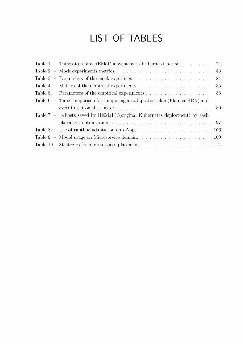
LIST OF TABLES

Table 1 – Translation of a REMaP movement to Kubernetes actions . . . . . . . . 74Table 2 – Mock experiments metrics . . . . . . . . . . . . . . . . . . . . . . . . . . 83Table 3 – Parameters of the mock experiment . . . . . . . . . . . . . . . . . . . . 84Table 4 – Metrics of the empirical experiments . . . . . . . . . . . . . . . . . . . . 85Table 5 – Parameters of the empirical experiments . . . . . . . . . . . . . . . . . . 85Table 6 – Time comparison for computing an adaptation plan (Planner HBA) and

executing it on the cluster. . . . . . . . . . . . . . . . . . . . . . . . . . 89Table 7 – (#hosts saved by REMaP)/(original Kubernetes deployment) by each

placement optimization. . . . . . . . . . . . . . . . . . . . . . . . . . . . 97Table 8 – Use of runtime adaptation on 𝜇Apps. . . . . . . . . . . . . . . . . . . . 106Table 9 – Model usage on Microservice domain. . . . . . . . . . . . . . . . . . . . 109Table 10 – Strategies for microservices placement. . . . . . . . . . . . . . . . . . . . 114

CONTENTS

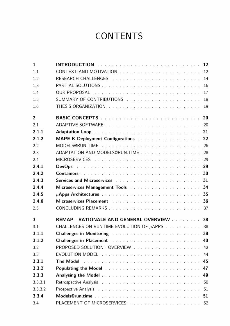
1 INTRODUCTION . . . . . . . . . . . . . . . . . . . . . . . . . . . . 121.1 CONTEXT AND MOTIVATION . . . . . . . . . . . . . . . . . . . . . . . 121.2 RESEARCH CHALLENGES . . . . . . . . . . . . . . . . . . . . . . . . . 141.3 PARTIAL SOLUTIONS . . . . . . . . . . . . . . . . . . . . . . . . . . . . 161.4 OUR PROPOSAL . . . . . . . . . . . . . . . . . . . . . . . . . . . . . . 171.5 SUMMARY OF CONTRIBUTIONS . . . . . . . . . . . . . . . . . . . . . 181.6 THESIS ORGANIZATION . . . . . . . . . . . . . . . . . . . . . . . . . . 19

2 BASIC CONCEPTS . . . . . . . . . . . . . . . . . . . . . . . . . . . 202.1 ADAPTIVE SOFTWARE . . . . . . . . . . . . . . . . . . . . . . . . . . . 202.1.1 Adaptation Loop . . . . . . . . . . . . . . . . . . . . . . . . . . . . . . 212.1.2 MAPE-K Deployment Configurations . . . . . . . . . . . . . . . . . . 222.2 MODELS@RUN.TIME . . . . . . . . . . . . . . . . . . . . . . . . . . . . 262.3 ADAPTATION AND MODELS@RUN.TIME . . . . . . . . . . . . . . . . . 282.4 MICROSERVICES . . . . . . . . . . . . . . . . . . . . . . . . . . . . . . 292.4.1 DevOps . . . . . . . . . . . . . . . . . . . . . . . . . . . . . . . . . . . 292.4.2 Containers . . . . . . . . . . . . . . . . . . . . . . . . . . . . . . . . . . 302.4.3 Services and Microservices . . . . . . . . . . . . . . . . . . . . . . . . 312.4.4 Microservices Management Tools . . . . . . . . . . . . . . . . . . . . 342.4.5 𝜇Apps Architectures . . . . . . . . . . . . . . . . . . . . . . . . . . . . 352.4.6 Microservices Placement . . . . . . . . . . . . . . . . . . . . . . . . . 362.5 CONCLUDING REMARKS . . . . . . . . . . . . . . . . . . . . . . . . . . 37

3 REMAP - RATIONALE AND GENERAL OVERVIEW . . . . . . . . 383.1 CHALLENGES ON RUNTIME EVOLUTION OF 𝜇APPS . . . . . . . . . . 383.1.1 Challenges in Monitoring . . . . . . . . . . . . . . . . . . . . . . . . . 383.1.2 Challenges in Placement . . . . . . . . . . . . . . . . . . . . . . . . . 403.2 PROPOSED SOLUTION - OVERVIEW . . . . . . . . . . . . . . . . . . . 423.3 EVOLUTION MODEL . . . . . . . . . . . . . . . . . . . . . . . . . . . . 443.3.1 The Model . . . . . . . . . . . . . . . . . . . . . . . . . . . . . . . . . 453.3.2 Populating the Model . . . . . . . . . . . . . . . . . . . . . . . . . . . 473.3.3 Analysing the Model . . . . . . . . . . . . . . . . . . . . . . . . . . . . 493.3.3.1 Retrospective Analysis . . . . . . . . . . . . . . . . . . . . . . . . . . . . 503.3.3.2 Prospective Analysis . . . . . . . . . . . . . . . . . . . . . . . . . . . . . 513.3.4 Models@run.time . . . . . . . . . . . . . . . . . . . . . . . . . . . . . . 513.4 PLACEMENT OF MICROSERVICES . . . . . . . . . . . . . . . . . . . . 52

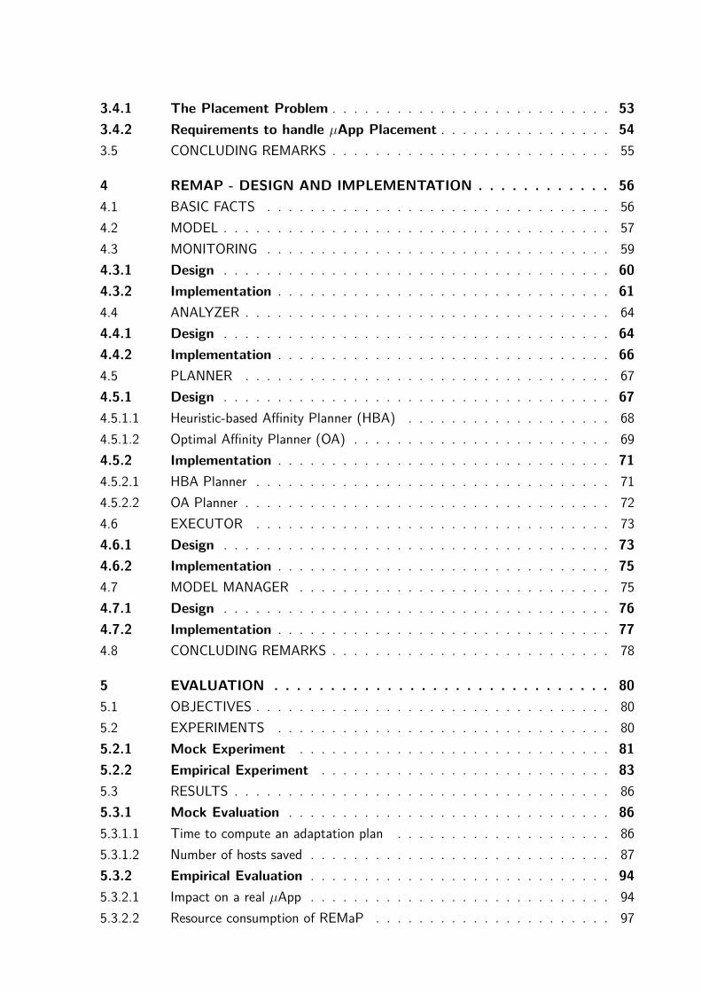
3.4.1 The Placement Problem . . . . . . . . . . . . . . . . . . . . . . . . . . 533.4.2 Requirements to handle 𝜇App Placement . . . . . . . . . . . . . . . . 543.5 CONCLUDING REMARKS . . . . . . . . . . . . . . . . . . . . . . . . . . 55

4 REMAP - DESIGN AND IMPLEMENTATION . . . . . . . . . . . . 564.1 BASIC FACTS . . . . . . . . . . . . . . . . . . . . . . . . . . . . . . . . 564.2 MODEL . . . . . . . . . . . . . . . . . . . . . . . . . . . . . . . . . . . . 574.3 MONITORING . . . . . . . . . . . . . . . . . . . . . . . . . . . . . . . . 594.3.1 Design . . . . . . . . . . . . . . . . . . . . . . . . . . . . . . . . . . . . 604.3.2 Implementation . . . . . . . . . . . . . . . . . . . . . . . . . . . . . . . 614.4 ANALYZER . . . . . . . . . . . . . . . . . . . . . . . . . . . . . . . . . . 644.4.1 Design . . . . . . . . . . . . . . . . . . . . . . . . . . . . . . . . . . . . 644.4.2 Implementation . . . . . . . . . . . . . . . . . . . . . . . . . . . . . . . 664.5 PLANNER . . . . . . . . . . . . . . . . . . . . . . . . . . . . . . . . . . 674.5.1 Design . . . . . . . . . . . . . . . . . . . . . . . . . . . . . . . . . . . . 674.5.1.1 Heuristic-based Affinity Planner (HBA) . . . . . . . . . . . . . . . . . . . 684.5.1.2 Optimal Affinity Planner (OA) . . . . . . . . . . . . . . . . . . . . . . . . 694.5.2 Implementation . . . . . . . . . . . . . . . . . . . . . . . . . . . . . . . 714.5.2.1 HBA Planner . . . . . . . . . . . . . . . . . . . . . . . . . . . . . . . . . 714.5.2.2 OA Planner . . . . . . . . . . . . . . . . . . . . . . . . . . . . . . . . . . 724.6 EXECUTOR . . . . . . . . . . . . . . . . . . . . . . . . . . . . . . . . . 734.6.1 Design . . . . . . . . . . . . . . . . . . . . . . . . . . . . . . . . . . . . 734.6.2 Implementation . . . . . . . . . . . . . . . . . . . . . . . . . . . . . . . 754.7 MODEL MANAGER . . . . . . . . . . . . . . . . . . . . . . . . . . . . . 754.7.1 Design . . . . . . . . . . . . . . . . . . . . . . . . . . . . . . . . . . . . 764.7.2 Implementation . . . . . . . . . . . . . . . . . . . . . . . . . . . . . . . 774.8 CONCLUDING REMARKS . . . . . . . . . . . . . . . . . . . . . . . . . . 78

5 EVALUATION . . . . . . . . . . . . . . . . . . . . . . . . . . . . . . 805.1 OBJECTIVES . . . . . . . . . . . . . . . . . . . . . . . . . . . . . . . . . 805.2 EXPERIMENTS . . . . . . . . . . . . . . . . . . . . . . . . . . . . . . . 805.2.1 Mock Experiment . . . . . . . . . . . . . . . . . . . . . . . . . . . . . 815.2.2 Empirical Experiment . . . . . . . . . . . . . . . . . . . . . . . . . . . 835.3 RESULTS . . . . . . . . . . . . . . . . . . . . . . . . . . . . . . . . . . . 865.3.1 Mock Evaluation . . . . . . . . . . . . . . . . . . . . . . . . . . . . . . 865.3.1.1 Time to compute an adaptation plan . . . . . . . . . . . . . . . . . . . . 865.3.1.2 Number of hosts saved . . . . . . . . . . . . . . . . . . . . . . . . . . . . 875.3.2 Empirical Evaluation . . . . . . . . . . . . . . . . . . . . . . . . . . . . 945.3.2.1 Impact on a real 𝜇App . . . . . . . . . . . . . . . . . . . . . . . . . . . . 945.3.2.2 Resource consumption of REMaP . . . . . . . . . . . . . . . . . . . . . . 97

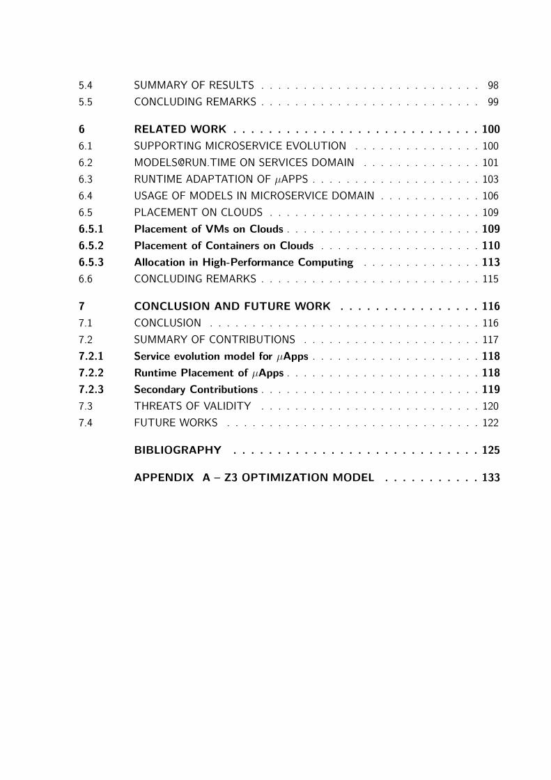
5.4 SUMMARY OF RESULTS . . . . . . . . . . . . . . . . . . . . . . . . . . 985.5 CONCLUDING REMARKS . . . . . . . . . . . . . . . . . . . . . . . . . . 99

6 RELATED WORK . . . . . . . . . . . . . . . . . . . . . . . . . . . . 1006.1 SUPPORTING MICROSERVICE EVOLUTION . . . . . . . . . . . . . . . 1006.2 MODELS@RUN.TIME ON SERVICES DOMAIN . . . . . . . . . . . . . . 1016.3 RUNTIME ADAPTATION OF 𝜇APPS . . . . . . . . . . . . . . . . . . . . 1036.4 USAGE OF MODELS IN MICROSERVICE DOMAIN . . . . . . . . . . . . 1066.5 PLACEMENT ON CLOUDS . . . . . . . . . . . . . . . . . . . . . . . . . 1096.5.1 Placement of VMs on Clouds . . . . . . . . . . . . . . . . . . . . . . . 1096.5.2 Placement of Containers on Clouds . . . . . . . . . . . . . . . . . . . 1106.5.3 Allocation in High-Performance Computing . . . . . . . . . . . . . . 1136.6 CONCLUDING REMARKS . . . . . . . . . . . . . . . . . . . . . . . . . . 115

7 CONCLUSION AND FUTURE WORK . . . . . . . . . . . . . . . . 1167.1 CONCLUSION . . . . . . . . . . . . . . . . . . . . . . . . . . . . . . . . 1167.2 SUMMARY OF CONTRIBUTIONS . . . . . . . . . . . . . . . . . . . . . 1177.2.1 Service evolution model for 𝜇Apps . . . . . . . . . . . . . . . . . . . . 1187.2.2 Runtime Placement of 𝜇Apps . . . . . . . . . . . . . . . . . . . . . . . 1187.2.3 Secondary Contributions . . . . . . . . . . . . . . . . . . . . . . . . . . 1197.3 THREATS OF VALIDITY . . . . . . . . . . . . . . . . . . . . . . . . . . 1207.4 FUTURE WORKS . . . . . . . . . . . . . . . . . . . . . . . . . . . . . . 122

BIBLIOGRAPHY . . . . . . . . . . . . . . . . . . . . . . . . . . . . 125

APPENDIX A – Z3 OPTIMIZATION MODEL . . . . . . . . . . . 133

12

1 INTRODUCTION

In this chapter we introduce our work. We present the context of microservices and theirunique characteristics, which motivate our desire to work with runtime adaptation onmicroservice-based applications (𝜇Apps). This chapter also presents the research’s chal-lenges on carrying out runtime adaptation on 𝜇Apps and how other initiatives have par-tially handled this issue. Next, we highlight our proposal and list our contributions inadapting 𝜇Apps at runtime.

1.1 CONTEXT AND MOTIVATIONAs business logic moves into the cloud (JAMSHIDI et al., 2018), developers need to or-chestrate not just the deployment of code to cloud resources but also the distribution ofthis code on the cloud platform. Cloud providers offer pay-as-you-go resource elasticityand a virtually infinite amount of resources, in which Microservice architectural style hasbecome an essential mechanism in order to take advantage of these features (NEWMAN,2015).

Architectural style tells us how to organize the code. It is the highest level of granu-larity and also specifies high level modules of an application as well as how they interactwith each other. On the other hand, architectural patterns solve problems related to thearchitectural style (e.g., the number of tiers a client-server architecture has - MVC).

In the Microservice architectural style, microservice-based applications (𝜇Apps) arebuild up by integrating many pieces of software, known as microservices, over a lightweightcommunication protocol.

A microservice (LEWIS; FOWLER, 2014) is a decoupled autonomic software that hasa specific function in a bounded context. It is intended role is to split the logic of anapplication into several smaller pieces of software, each with a single and specific role,integrated with lightweight general purpose communication protocols (e.g., HTTP).

Despite the many similarities between services and microservices (ZIMMERMANN,2016), there are some fundamental differences between them, mainly related to theirexecution. Languages like WS-BPEL (JORDAN; EVDEMON, 2007) describe service compo-sitions workflow while a microservice-based application (𝜇App) workflow is not formallyspecified. The 𝜇App communication must be monitored to infer the underlying workflowand to change its behaviour it is necessary to upgrade the application, deploying differentmicroservices.

The flexibility of 𝜇Apps made microservices the favourite architectural style for de-ploying complex application logic. Companies such as Amazon and Netflix have hundreds

Chapter 1. Introduction 13

of different microservices in their applications. Amazon1 uses approximately 120 microser-vices to generate one page whereas Uber2 manages 1000s of microservices and Netflix3

has more than 600 microservices in its application.The decoupling and well-defined interfaces provide the ability for 𝜇Apps to scale in-

/out seamlessly and allowing developers to perform upgrades by deploying new serviceversions without halting the 𝜇App. In addition to this, decoupling allows microservicesto be developed by using different technology stacks or by changing it along the 𝜇App’slifespan. Development teams can use or add new technologies to better fulfill the applica-tion’s requirements, improving its security and reliability through frequent updates (e.g.applying bug fixes on the chosen stack), resulting in frequent component deployments.

A downside, however, of using microservices is managing their deployments. Microser-vices that compose an application can interact and exchange a significant amount of dataat runtime, creating communications between them affinities (CHEN et al., 2013). Theseinter-service affinities can have a substantial impact on the performance of 𝜇Apps depend-ing on the placement of the microservices. High-affinity microservices, for example, willhave a worse performance due to higher communication latency when placed on differenthosts. Another fact which makes this scenario worse is the change in affinities at runtimeas consequence of the frequent upgrades in a 𝜇App.

Along with affinities, developers must also account for the microservice’s resource usagein order to optimize the 𝜇App’s performance. Microservices with high resource usage, forexample, should not be placed on the same host.

Existing management tools, such as Kubernetes4, allow development-operations (De-vOps) engineers to control 𝜇Apps by setting resource thresholds on the microservices.Management tools uses this information to decide when to scale in/out each microserviceand where to place microservice replicas. At runtime, the management tools continu-ously compare the instantaneous resource usage of the microservices with their resourcethreshold. When the resource usage reaches a given limit, the management tool starts thescaling action. Existing management tools select in which hosts to place the microservicesreplicas during scale out, based on the set thresholds instead of their real resource usage.In most cases, the threshold is unrealistic and leads the 𝜇App to waste cluster resourcesor to lose performance due to resource contention.

𝜇Apps management is automatized by tools that monitor and analyze their behavioras well as apply adaptation actions in response to specific conditions at runtime. Thesetools are fundamental in handling 𝜇Apps, especially those with a significant amount ofmicroservices; however, they are not fully autonomous. They are unaware of informationabout the 𝜇App context, making human intervention necessary in some management1 <http://highscalability.com/amazon-architecture>2 <https://www.youtube.com/watch?v=BT9sUm5M77y>3 <https://www.infoq.com/presentations/migration-cloud-native>4 <https://kubernetes.io/>

Chapter 1. Introduction 14

activities such as monitoring and analysis.During a 𝜇App’s execution, management tools are only aware of the current snapshot

of the application’s resource usage and few static configurations, set by the engineersduring the 𝜇App’s deployment. Behavioural information such as messages - exchanged bymicroservices -, their logs and resource usage history is not considered. Hence, to carryout a sophisticated and graceful management at runtime, engineers need to analyze thesedifferent sorts of data and manually apply an adaptation action in response to the results.

The lack of behavioural awareness comes from the heterogeneity of the microservices,which make it difficult to use a general purpose approach to inspect 𝜇Apps at runtime.Different languages used in the development of microservices impose a semantic gap incollecting runtime data generated by the 𝜇App. A single 𝜇App may have different monitorsto gather resource usage metrics from microservices in different languages, for example;in this case each tool has its own data format and semantic. It is the role of the engineerto handle these differences when analyzing the data. To gather other sorts of data, suchas the logs and messages, additional monitoring tools are necessary; different from thoseused to collect resource metrics.

To make matters worse, frequent updates and upgrades to 𝜇Apps make their behaviourchange continuously; leaving engineers to face dynamic behavior despite all the challengesto monitor and analyze the heterogeneous data generated. This mutable behaviour forcesthe continuous monitoring and analysis of 𝜇Apps in order to avoid flaws at runtime;solving them as fast as possible if they come up.

These varied and mutable characteristics overwhelm the engineers - imposing a highcost in managing the 𝜇Apps- making it challenging to make decisions in order to con-trol the 𝜇App and consequently making management slow, error-prone and with poorresults (HOFF, 2014; KILLALEA, 2016; SINGLETON, 2016)

An example of poor 𝜇App management is placing microservices in a cluster. To deploya 𝜇App engineers might set a minimum amount of resources that the microservices need tobootstrap. At runtime, on the other hand, the resource usage history in some microservicesin the 𝜇App have different values from the ones set by the engineers; management tools,however, are not aware of this runtime behavior.

1.2 RESEARCH CHALLENGES𝜇Apps have a dynamic behaviour. The high decoupling among their microservices allowsengineers to apply updates and upgrades easily without the need to halt the whole 𝜇App;making frequent updates and upgrades in a short time span common. Compared to otherarchitectural styles in general, a 𝜇App can change many times throughout a day, to whichit is defined as an inherent runtime adaptive system.

𝜇App engineers apply adaptations mostly manually, underusing the adaptive potential

Chapter 1. Introduction 15

of these applications. In general, engineers observe the application log and metric chartslooking for a situation that needs to be changed in the running 𝜇App. They then settriggers to update the application (e.g. scale in/out a set of microservices) or manuallyapply an upgrade (e.g. roll out/back a microservice version). Hence, changes to 𝜇Appsrely on the management of their microservices. Adaptations are mostly structural andmust deal with the placement of the microservices onto the cluster.

Manual intervention on 𝜇Apps is a consequence of the challenges for monitoring anddeciding over the data generated by the 𝜇App. The heterogeneity of the tools used forgathering data, the lack of a well-defined structure for the generated data, is the primarychallenge on automatizing the adaptation in 𝜇Apps.

Moreover, managing microservices in a cluster is a hard task. In order to place amicroservice in a cluster, it is necessary to match the requirements of the microserviceto the features available in a cluster node. It is a classic optimization problem of multi-dimensional bin-packing that it is hard to be applied at runtime due to its NP-Hardcomplexity. Management tools usually have generic strategies to place microservices inthe cluster, but this placement it is not optimal, it wastes resources and threatens the𝜇App’s performance.

In this context, the main objective of this thesis is:

To automatize the adaptation of 𝜇Apps, improving the placement ofmicroservices at runtime.

Along to this work, we explain that runtime adaptation of 𝜇Apps relies on to in-stantiate (new) microservices somewhere in the cluster. Hence, we aiming to handle thechallenges for improving the placement of microservices an runtime. We reach the im-provement by optimizing the location of microservices based on their behavior – historyresources usage and messages exchanged (𝜇App workflow).

To bring automation to adapt 𝜇Apps, we must cope with three activities based onMAPE-K architecture (IBM, 2005):

1. to observe the application (monitoring);

2. to decide what to do (analysis and planning); and,

3. to perform an action (execution).

However, there are some challenges for carrying out these activities in the 𝜇App do-main. Next, we overview these challenges:

Challenge 1: Unified monitoring of 𝜇Apps. Existing management tools can collectand expose many resource metrics from executing 𝜇Apps. However, each 𝜇App usesits own monitoring stack. The diversity of monitoring options create a semanticchallenge, which requires a single unified data model in order to be solved.

Chapter 1. Introduction 16

Challenge 2: Finding a high-performing placement. Microservices are usually placedusing static information such as available host resources. However, this strategy riskslowering 𝜇App performance by putting high-affinity microservices on different hostsor by co-locating microservices with high resource usage. Hence, it is necessary tofind the best performing configuration that maps microservices to servers. This leadsto two sub-problems:

1. An ample space of configurations: with 𝑛 servers and 𝑚 microservices thereare 𝑚𝑛 possible configurations; and,

2. The performance of a 𝜇App configuration changes dynamically.

Challenge 3: Migrating microservices. Existing microservice management tools donot expose any means to perform live migration of microservices between hosts. Livemigration is necessary to provide seamless runtime adaptation.

These challenges raise the question:

Can we optimize the placement of microservices by carrying out autonomousmanagement based on the behavioural data of the 𝜇Apps?

However,

How to bring autonomy to 𝜇App management despite the several challengesin monitoring heterogeneous microservices?

Therefore, in this thesis we answer this question by introducing REMaP (RuntimEMicroservices Placement) an autonomous adaptation manager for 𝜇Apps with mini-mum human intervention. The autonomous management observes 𝜇Apps at runtime andsmartly places microservices onto the cluster, thus improving performance and decreasingthe waste of resources by 𝜇Apps.

1.3 PARTIAL SOLUTIONSFew papers aim to bring autonomy for the management of 𝜇Apps. Florio and Nitto(2016) propose an independent mechanism, named Gru, to change the 𝜇App deploymentat runtime to provide runtime scaling. Gru auto-scales microservices based on CPU andmemory usage as well as microservice response time. However, this approach is techno-logically locked and only works on Docker5. Moreover, it is out of the scope of Gru toinspect runtime behaviour of microservices (i.e. 𝜇App workflow) to change the 𝜇App.5 <https://www.docker.com>

Chapter 1. Introduction 17

Rajagopalan and Jamjoom (2015) propose App-Bisect – an autonomous mechanismto update a running deployment to a different version. App-Bisect monitors the 𝜇Appalong their execution, tracking the upgrades of microservices. When App-Bisect detectsa poor performance of the 𝜇App after an upgrade, it reverts some microservices in theapplication to earlier versions thus solving the performance issue. This approach aims toimprove the performance by reverting the configuration of the 𝜇App. Again, this approachalso does not analyze the behaviour of the 𝜇App neither the microservices interactions inorder to change it.

1.4 OUR PROPOSALTo handle the challenges of optimizing the placement of microservices, we are proposingan adaptation manager structured as a control loop feedback – in which the performanceis centered on the use of runtime models and verification as well as optimization strategies– to make practical runtime adaptations to the 𝜇Apps.

We abstract the heterogeneity of microservices domain in a model at runtime thatmaintains information related to the 𝜇Apps behaviour. The model is the knowledge sourceused by the control loop in the monitoring, analysis, planning and adaptation activities.

To show the feasibility of our approach, we use the execution environment to computea quasi-optimal placement of a 𝜇App based on its runtime behaviour. This computedplacement aims to decrease the number of hosts used by the 𝜇App and can, in specificcases, improve the performance of the 𝜇App.

The focus of our work it to carry out a model-driven runtime adaptation on 𝜇Apps.To demonstrate our adaptation approach, we should decrease the 𝜇App resource usage byautomatically reconfiguring the placement of microservices at runtime, based on onlinemonitoring of the 𝜇App, without compromising 𝜇App performance. We do so by usingan adaptation mechanism that solves the challenges above and automatically changesthe placement of microservices by using their affinities and resource usage. Our solutionuses a MAPE-K based (IBM, 2005) adaptation manager to upgrade the placement of𝜇Apps at runtime autonomously. The adaptation manager uses Models@run.time (BLAIR;

BENCOMO; FRANCE, 2009) concepts to abstracts the diversity of monitoring stacks andmanagement tools and guide the adaptation. In doing so our solution provides a unifiedview of the cluster and the 𝜇Apps running under the adaptation manager.

The adaptation manager groups and places microservices with high affinity on thesame physical server – this strategy contrasts with existing static approaches, which relyon information provided by engineers before 𝜇App deployment. Hence, our adaptationmanager can provide resources based on actual microservice resource utilization, avoidingresource contention/waste during 𝜇App execution. Moreover, the co-location of microser-vices decreases the impact of network latency on the 𝜇App workflow, which improves

Chapter 1. Introduction 18

overall application performance. At the end of the adaptation the 𝜇App is in an opti-mized configuration, which reduce the number of hosts needed to execute the 𝜇App andcan improve its performance in comparison to a static configuration.

We evaluated our adaptation mechanism in two scenarios, using three strategies: oneheuristic-based and two based on SAT-Solvers (BIERE et al., 2009). In the first scenario weused the proposed mechanism to compute the adaptation of synthetic application graphs,having a different number of microservices and affinities. In this scenario, we conductedadaptations that saved up to 85% of the hosts initially used by the 𝜇Apps. This evaluationshows that our approach produces better results on 𝜇Apps with a dense topology graph.Moreover, strategies chosen to optimize the placement by using SAT-Solvers were unableto work in large 𝜇Apps (with more than 20 microservices); hence – despite the fact thatour heuristic cannot guarantee an optimal result – it was able to compute new placementsfor any size of 𝜇App.

In the second scenario we used the proposed mechanism to adapt a benchmark 𝜇App6

running on Azure. In this scenario we achieved a performance improvement of 3% andsaved 20% of hosts used in the initial deployment. Moreover, we found that a poor place-ment that uses the same number of hosts can decrease the overall performance of the𝜇App by 4x, indicating that the placement requires special care by engineers – which ourapproach automates.

1.5 SUMMARY OF CONTRIBUTIONSThis thesis makes several contributions to runtime adaptation of 𝜇Apps. Next, we listthese main contributions.

The definition of runtime adaptation of 𝜇Apps : This thesis systematizes whatthe adaptation of 𝜇Apps is, as well as the challenges of applying it at runtime.

The use of models for supporting the evolution of microservices : The numberof technologies used to build up a 𝜇App; the frequency of 𝜇App changes – due toupdates and upgrades – as well as the number of microservices and microservicereplicas; make it complex to track their evolution. Therefore, we contribute to adiscussion about how models can be used to support the evolution of 𝜇Apps andpropose two models to adapt microservices.

The use of affinities to drive runtime adaptation on 𝜇Apps : In addition to re-sources available in a cluster, the behaviour of a 𝜇App can affect its performance.Therefore, we propose the concept of affinities to define the degree of relationship be-tween two microservices; by co-locating high related microservices, we can improvethe overall performance of the application.

6 <https://microservices-demo.github.io>

Chapter 1. Introduction 19

Strategy to rearrange microservices at runtime : to reconfigure microservices in acluster – to optimize the 𝜇App performance – and the resource usage in an NP-Hardtask, in many cases, cannot be computed in a reasonable amount of time. Therefore,we use the concept of affinities during the adaptation to improve the placement ofmicroservices to achieve (quasi-)optimal configurations.

A MAPE-K based adaptation mechanism for adapting 𝜇Apps at runtime : Adap-tation mechanism for 𝜇Apps usually rely on metrics to change their configuration.In this thesis, we contribute by presenting an adaptation mechanism that relies ona runtime model of the 𝜇App to guide its adaptation. Instead of observing onlymetrics such as CPU and memory usage, our approach observes the behaviour ofthe 𝜇App through the interaction among their microservices, which allows moreeffective adaptations at runtime.

1.6 THESIS ORGANIZATIONThe following thesis is organized as follows. Chapter 2 presents the basic concepts usedthroughout the thesis, namely: adaptive software; models and Models@run.time in run-time adaptation; and microservices.

Chapter 3 discusses the rationale and general overview of our approach; presents thechallenges on runtime evolution of 𝜇Apps; introduces our solution and our approach tosupport 𝜇App evolution by using models and discusses the challenges on the placementof 𝜇Apps. Chapter 4 shows the design and implementation of REMaP. It initiates withan overview of REMaP– describing the model used by REMaP during the adaptationof 𝜇Apps– and presents details of the design and implementation of MAPE-K basedcomponents: Monitoring, Analyzer, Planning, Execution.

Chapter 5 presents the evaluation of our solution and results. Section 5.3.1 we presentthe results of the mock evaluation and in Section 5.3.2 we present the results of theempirical evaluation. Chapter 6 is an overview of the related work, positioning our work infive categories: supporting microservices evolution, Models@run.time on services domain,runtime adaptation of 𝜇Apps, usage of models in microservice domain, and placement onclouds.

Finally, presents a summary of the results obtained; discusses our contributions; showsthe limitations of our approach and how we aim to extend this work discussing futureworks.

20

2 BASIC CONCEPTS

In this chapter we present the primary concepts used throughout the rest of this thesis.We begin by describing the ideas of autonomic computing and adaptive software, high-lighting the reference architecture MAPE-K – to develop adaptive software – and themain strategies to deploy MAPE-K in order to manage an underneath system. Moreover,we describe how the use of models facilitate system adaptation. Next we present the no-tion of models and their use at runtime. Furthermore, we present the motivation behindmicroservices; their fundamental concepts and how microservices are comparable to ser-vices. To conclude, we also present management tools for microservice-based applications(𝜇Apps) and the challenges in correctly placing microservices in the cluster.

2.1 ADAPTIVE SOFTWAREAdaptive software are those capable of change in order to satisfy requirements. The adap-tation is achieved, in most cases, through autonomic computing (KEPHART; CHESS, 2003).Autonomic computing refers to self-managing computing systems (HUEBSCHER; MCCANN,2008) – the system controls itself. In self-managed systems human intervention is not nec-essary in activities such as optimization, healing, protection, and configuration. The sys-tem management is achieved by changing (adapting) some of its structural or behavioralaspects in response to internal or external stimuli.

A self-managed (or self-adaptive) system must monitor it’s own signals – as well asthe environment’s – as well as analyze and apply actions in response to them – perhapsby modifying itself. These steps repeat themselves indefinitely as a control loop. Fourfacts (KELING; DALMAU; ROOSE, 2012) usually motivate changes in the system:

1. Changes of environment’s conditions: When the infrastructure, where the system isdeployed, changes due to updates or failures the system must adapted in order todeal with them without completely stopping;

2. Changes of application requirements: When application requirements change, in re-silience or performance, the application must be updated in order to satisfy the newrequirements.

3. Detection of bugs: When bugs are detected, the application must be updated to fixthem, thus avoiding possible outages.

4. Application evolution: When a new version of a component is developed the appli-cation is updated by replacing the current version of the component with a newone.

Chapter 2. Basic Concepts 21

These adaptations can be corrective, evolutionary or reactive (KELING; DALMAU;

ROOSE, 2012). A corrective adaption is performed when a problem is diagnosed in theenvironment or system itself; an evolutionary adaption is performed to update a systemin order to better satisfy the requirements of the system or to use new implementationsor technologies; and a reactive adaption is carried out to respond to a specific monitoredevent.

Adaptation performed in the application can be structural or behavioural (KELING;

DALMAU; ROOSE, 2012). As its name suggests, a structural adaption changes the structureof the application by adding, removing, replacing and reconnecting components. Mean-while, a behavioural adaption changes the behaviour of the system by adding/removingfunctionalities or changing some configuration parameter.

In both cases, the structure of the adaption process consists of a control loop. Themost relevant examples of control loops are Rainbow (GARLAN et al., 2004) and MAPE-K (KEPHART; CHESS, 2003). IBM systematized MAPE-K as a reference model for au-tomatic control loops (IBM, 2005). MAPE-K organizes the adaptation process in fourphases: monitoring, analysis, planning, and execution.

2.1.1 Adaptation Loop

Autonomous mechanisms carry out adaptations in a system by sensing signals from theenvironment and/or from the system itself; the autonomous mechanism decides what todo; and acts over the managed system. This sequence of steps repeat indefinitely as a loopnamed control loop or adaptation loop.

In self-adaptive systems, the adaptation loop is part of the system, whereas, in su-pervised adaptive systems, the process to diagnose and select an adaption is placed in athird-party element.

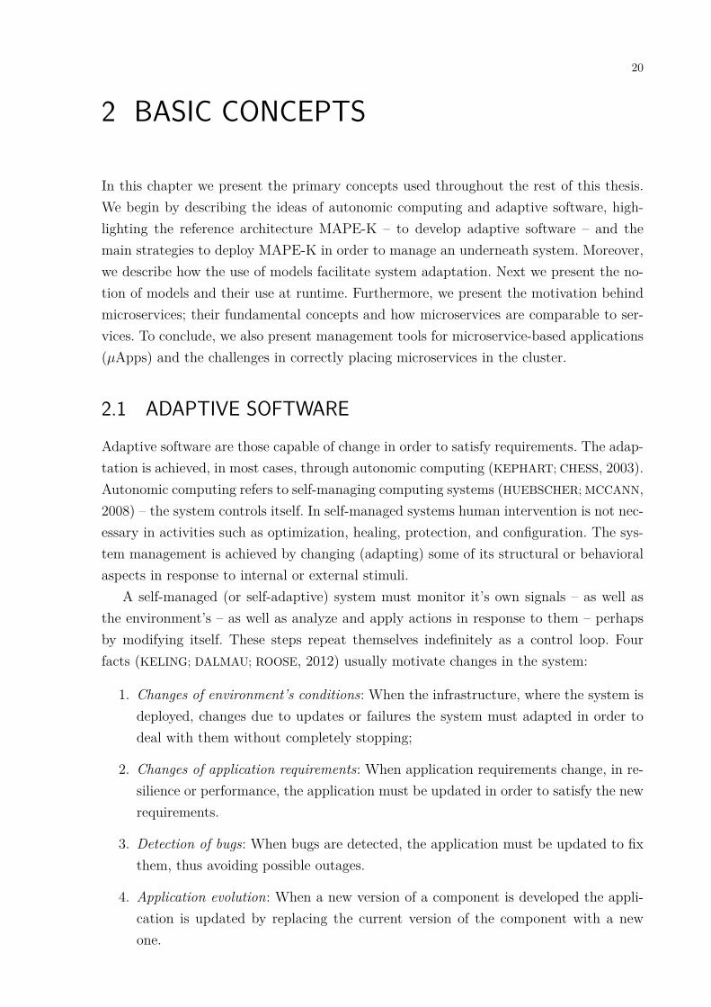
In MAPE-K framework, the adaption loop is made up by four stages as shown inFIG. 1: monitoring, analysis, planning and execution. Salehie and Tahvildari (2009) definethese activities as follows:

• Monitoring: The monitoring stage is responsible for collecting and correlating datafrom sensors and converting them into behavioural patterns and symptoms, whichcan be done through event correlation and threshold checking. MAPE-K senses amanaged system through sensors, and sends the collected data to a monitor. Themonitor then aggregates the received data as symptoms that should be analyzed.

• Analysis: This activity is responsible for the analysis of the symptoms – provided bythe monitoring stage and the system history – in order to detect when a change isrequired. If a change is required, the analyzer generates a change request and passesit to the planner.

Chapter 2. Basic Concepts 22

Figure 1 – MAPE-K framework for developing adaptation loops.

Managed System

Monitoring Executing

PlanningAnalysis

KnowledgeBase

Source: (IBM, 2005)

• Planning: The planning activity determines what needs to be changed and what isthe best to carry it out. In MAPE-K, the planner creates/selects a procedure toapply a desired adaptation in the managed resource and passes it to the executoras an adaptation (change) plan.

• Execution: The execution stage is responsible for applying the actions determined inthe planning stage. It includes managing non-primitive actions through predefinedworkflows, or mapping actions, to what is provided by actuators and their underly-ing dynamic adaptation mechanisms. The actuator allows the executor to performactions to change the managed resource.

Lastly, MAPE-K activities of share a knowledge base that maintains rules, properties,models and other kinds of data, used to steer how to provide autonomy to the underlyingsystem.

2.1.2 MAPE-K Deployment Configurations

In the adaptation of distributed systems, several deployment configurations can be appliedon MAPE-K to better compute the adaptation plan without degrading the performanceor threatening the execution of its managed system. Weyns et al. (2013) categorizes thedeployment of MAPE-K architectures into local, remote, centralized and decentralized.Next, we present these deployments patterns and their main variations.

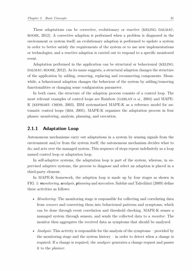
In a local deployment, FIG. 2, all components of MAPE-K run on the same host as themanaged application. An advantage of this deployment is that no messages are exchangedbetween monitored microservices and the MAPE-K instance. The disadvantage is thatboth the application and the control-loop contend for the same local machine resources –

Chapter 2. Basic Concepts 23

such as CPU and memory. Another issue with a local deployment is that MAPE-K lacksa global view of the application if it’s components are deployed across several hosts.

Figure 2 – MAPE-K local deployment.

Source: Adapted from (WEYNS et al., 2013)

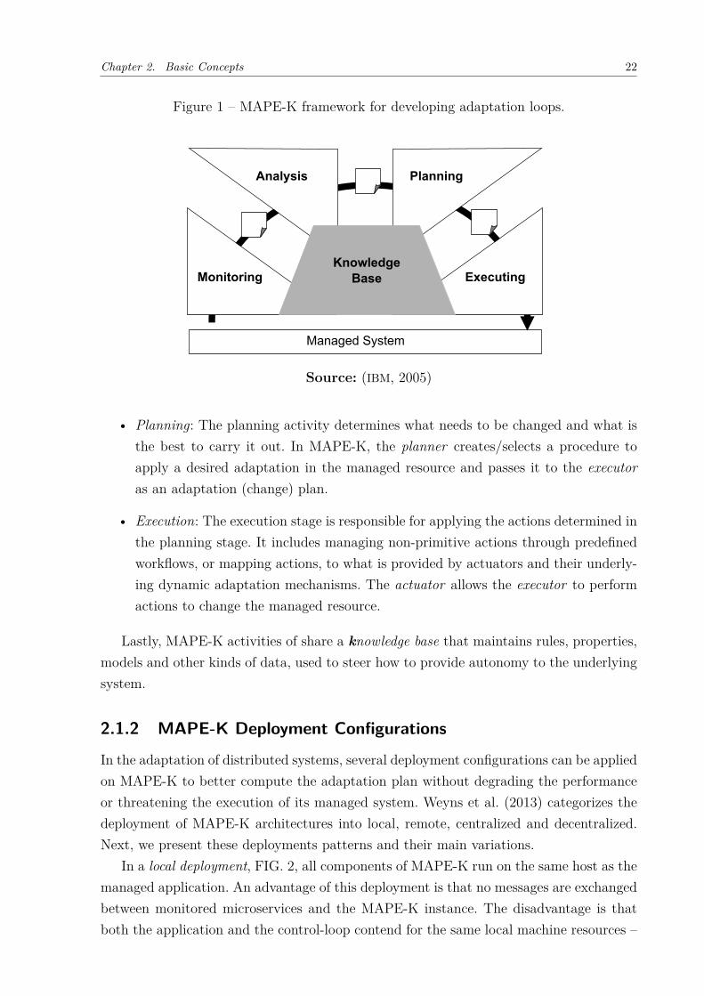
In a remote deployment, as shown in FIG. 3, components that implement MAPE-K activities and the managed application run in different hosts making it necessary formonitored messages and adaptation actions to traverse the network, which incurs latency.If this latency is sufficiently high, it can jeopardize the time taken to apply an action inresponse to a violation and may be unacceptable. The advantage of a remote deployment isthat MAPE-K can construct a global view of all components that compose the application.

Figure 3 – MAPE-K remote deployment.

Host A Host B

MAPE

Source: Adapted from (WEYNS et al., 2013)

In a centralized deployment, as shown in FIG. 4, all the components that implementthe MAPE-K activities are in a single host. A key disadvantage of centralization is thatit introduces a single point of failure; leaving potential for performance degradation onceeach stage of MAPE-K competes for the same resources.

It is also possible to deploy a remote centralized MAPE-K instance. However, if theapplication is deployed across several hosts, the MAKE-K instance may be local to onlya few application components and remote to others. In this hybrid approach, in caseof frequently updated components, there is no guarantee that the host location whereMAPE-K is deployed will be the same as the one where the application components arerunning.

A decentralized deployment can be divided into two cases:

1. Several instances of MAPE-K: several MAPE-K instances distributed acrossseveral hosts; and

Chapter 2. Basic Concepts 24

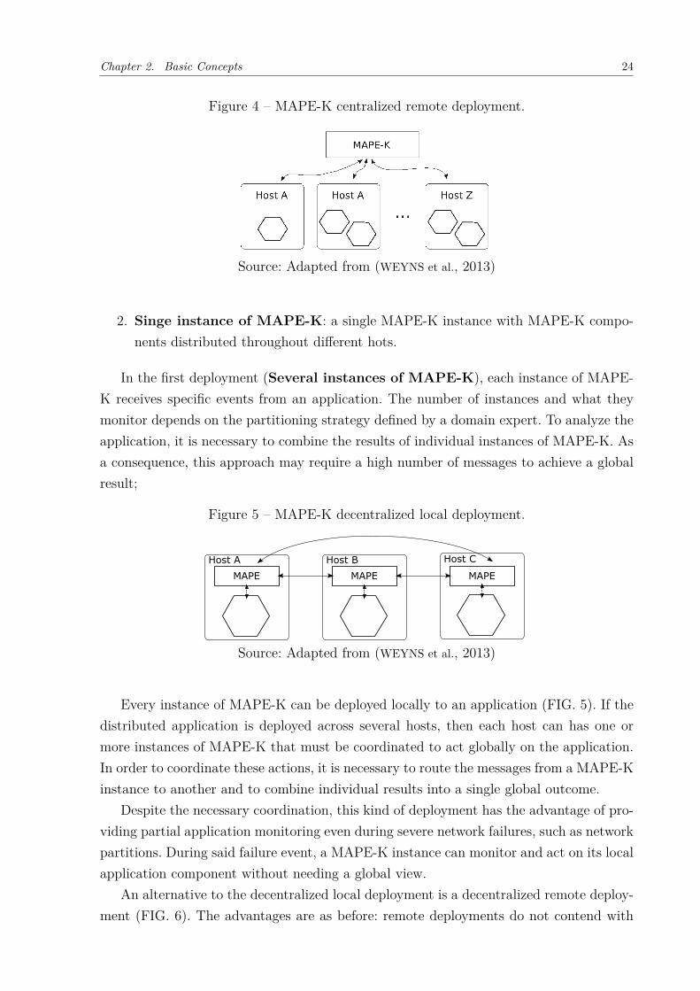
Figure 4 – MAPE-K centralized remote deployment.

...Host A Host A Host Z

MAPE-K

Source: Adapted from (WEYNS et al., 2013)

2. Singe instance of MAPE-K: a single MAPE-K instance with MAPE-K compo-nents distributed throughout different hots.

In the first deployment (Several instances of MAPE-K), each instance of MAPE-K receives specific events from an application. The number of instances and what theymonitor depends on the partitioning strategy defined by a domain expert. To analyze theapplication, it is necessary to combine the results of individual instances of MAPE-K. Asa consequence, this approach may require a high number of messages to achieve a globalresult;

Figure 5 – MAPE-K decentralized local deployment.

MAPE

Host A

MAPE

Host B

MAPE

Host C

Source: Adapted from (WEYNS et al., 2013)

Every instance of MAPE-K can be deployed locally to an application (FIG. 5). If thedistributed application is deployed across several hosts, then each host can has one ormore instances of MAPE-K that must be coordinated to act globally on the application.In order to coordinate these actions, it is necessary to route the messages from a MAPE-Kinstance to another and to combine individual results into a single global outcome.

Despite the necessary coordination, this kind of deployment has the advantage of pro-viding partial application monitoring even during severe network failures, such as networkpartitions. During said failure event, a MAPE-K instance can monitor and act on its localapplication component without needing a global view.

An alternative to the decentralized local deployment is a decentralized remote deploy-ment (FIG. 6). The advantages are as before: remote deployments do not contend with

Chapter 2. Basic Concepts 25

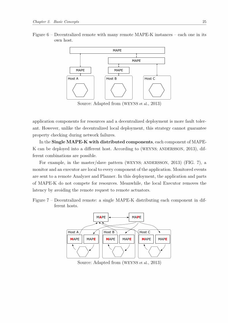
Figure 6 – Decentralized remote with many remote MAPE-K instances – each one in itsown host.

Host A Host B Host C

MAPE MAPE

MAPE

MAPE

Source: Adapted from (WEYNS et al., 2013)

application components for resources and a decentralized deployment is more fault toler-ant. However, unlike the decentralized local deployment, this strategy cannot guaranteeproperty checking during network failures.

In the Single MAPE-K with distributed components, each component of MAPE-K can be deployed into a different host. According to (WEYNS; ANDERSSON, 2013), dif-ferent combinations are possible.

For example, in the master/slave pattern (WEYNS; ANDERSSON, 2013) (FIG. 7), amonitor and an executor are local to every component of the application. Monitored eventsare sent to a remote Analyzer and Planner. In this deployment, the application and partsof MAPE-K do not compete for resources. Meanwhile, the local Executor removes thelatency by avoiding the remote request to remote actuators.

Figure 7 – Decentralized remote: a single MAPE-K distributing each component in dif-ferent hosts.

Host A

MAPE MAPE

Host B

MAPE MAPE

Host C

MAPE MAPE

MAPE MAPE

Source: Adapted from (WEYNS et al., 2013)

Chapter 2. Basic Concepts 26

2.2 MODELS@RUN.TIMEModel Driven Engineering (MDE) (SCHMIDT, 2006) is an approach used in Software Engi-neering for specification, construction, and system maintenance. MDE aims to systematizethe use of models so that they can be used for different objects along all activities in thesoftware development process – including software execution. Models are therefore usednot only during the specification and development phases or for documentation and codegeneration purposes, but also as a live element to maintain the state of the system (soft-ware and its environment) – keeping its structure and behaviour, as well as for guidingthe system execution.

A model is a high-level representation of the system in which technical details are ab-stracted in favour of domain-specific and technology agnostic information. This approachseparates concerns between the technology used for the system implementation and itsbusiness logic (PARVIAINEN et al., 2009), facilitating the development and maintenance ofthe modelled system.

Models are used to simplify the representation of complex systems. The model is ahigh-level view that only exposes the relevant structure and behaviour of the systemaccording to the model’s usage intent.

A manually created model (user-defined model) is usually drawn up by the applica-tion engineer in a top-down approach. The user observes aspects of the domain, removinguseless information – given the context and purpose of the model –, and organizes allinformation respecting the model rules. User-defined models usually help the construc-tion (NÚÑEZ-VALDEZ et al., 2017) and integration (YU et al., 2015) of systems – automaticcode generation and interoperability – or for controlling the behaviour (SAMPAIO JR.;

COSTA; CLARKE, 2013) – maintaining control policies to guide the system execution.An automatically created model, on the other hand, (emergent model) is drawn up

in a bottom-up approach. The model emerges from metrics, execution traces and severalother system signals. Dedicated tools – specialized for a domain – collect all data andorganize them into the model.

A model is drawn up by using its meta-model (see FIG. 8), which is the abstractionfor building a model and has elements that say what can be expressed and how theyare structured in the model. The characteristics of a domain are captured into the meta-model allowing it to be used for instantiating different models of the same domain. Likean object that is an instance of a class in the object-oriented paradigm, a model is aninstance of a meta-model in MDE.

The meta-model is usually defined for a specific domain. The domain specialist de-termines which are the main elements and their meanings as well as how these elementsshould be organized in the model in order to best represent a particular domain. All thisinformation is then compiled into the meta-model, guiding it on how to draw up themodel.

Chapter 2. Basic Concepts 27

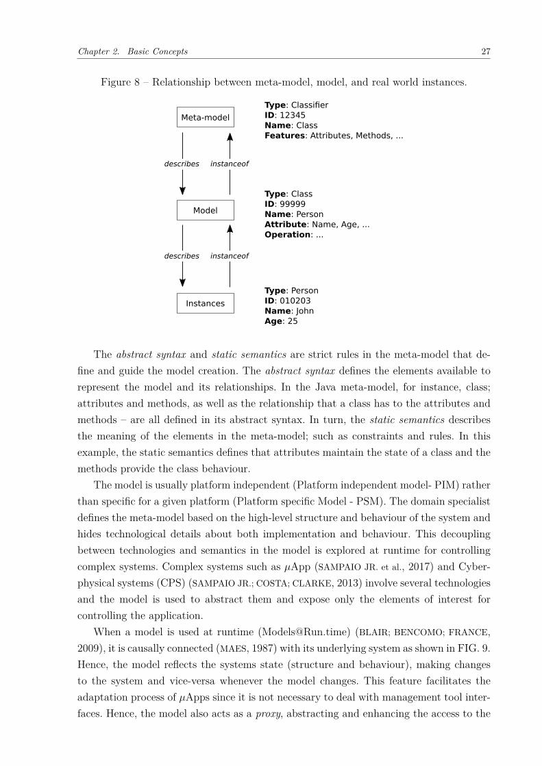
Figure 8 – Relationship between meta-model, model, and real world instances.

Meta-model

Type: ClassifierID: 12345Name: ClassFeatures: Attributes, Methods, ...

Model

Type: ClassID: 99999Name: PersonAttribute: Name, Age, ...Operation: ...

Instances

Type: PersonID: 010203Name: JohnAge: 25

describes instanceof

describes instanceof

The abstract syntax and static semantics are strict rules in the meta-model that de-fine and guide the model creation. The abstract syntax defines the elements available torepresent the model and its relationships. In the Java meta-model, for instance, class;attributes and methods, as well as the relationship that a class has to the attributes andmethods – are all defined in its abstract syntax. In turn, the static semantics describesthe meaning of the elements in the meta-model; such as constraints and rules. In thisexample, the static semantics defines that attributes maintain the state of a class and themethods provide the class behaviour.

The model is usually platform independent (Platform independent model- PIM) ratherthan specific for a given platform (Platform specific Model - PSM). The domain specialistdefines the meta-model based on the high-level structure and behaviour of the system andhides technological details about both implementation and behaviour. This decouplingbetween technologies and semantics in the model is explored at runtime for controllingcomplex systems. Complex systems such as 𝜇App (SAMPAIO JR. et al., 2017) and Cyber-physical systems (CPS) (SAMPAIO JR.; COSTA; CLARKE, 2013) involve several technologiesand the model is used to abstract them and expose only the elements of interest forcontrolling the application.

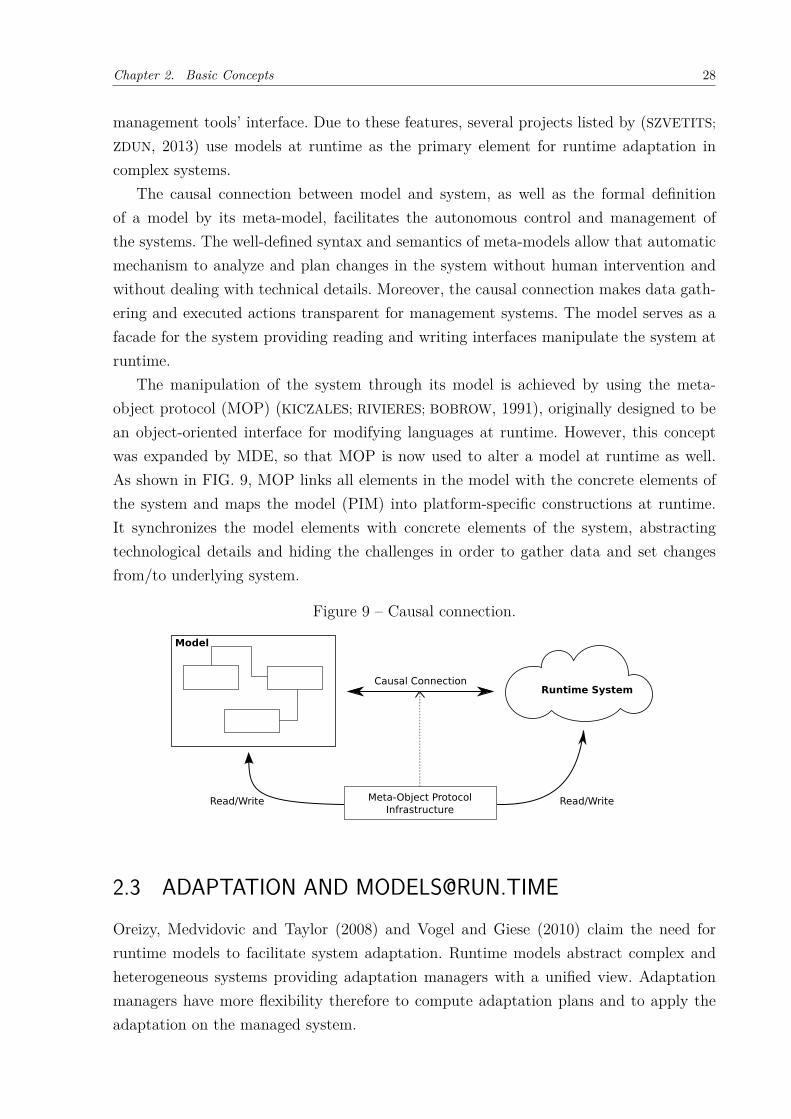
When a model is used at runtime (Models@Run.time) (BLAIR; BENCOMO; FRANCE,2009), it is causally connected (MAES, 1987) with its underlying system as shown in FIG. 9.Hence, the model reflects the systems state (structure and behaviour), making changesto the system and vice-versa whenever the model changes. This feature facilitates theadaptation process of 𝜇Apps since it is not necessary to deal with management tool inter-faces. Hence, the model also acts as a proxy, abstracting and enhancing the access to the

Chapter 2. Basic Concepts 28

management tools’ interface. Due to these features, several projects listed by (SZVETITS;

ZDUN, 2013) use models at runtime as the primary element for runtime adaptation incomplex systems.

The causal connection between model and system, as well as the formal definitionof a model by its meta-model, facilitates the autonomous control and management ofthe systems. The well-defined syntax and semantics of meta-models allow that automaticmechanism to analyze and plan changes in the system without human intervention andwithout dealing with technical details. Moreover, the causal connection makes data gath-ering and executed actions transparent for management systems. The model serves as afacade for the system providing reading and writing interfaces manipulate the system atruntime.

The manipulation of the system through its model is achieved by using the meta-object protocol (MOP) (KICZALES; RIVIERES; BOBROW, 1991), originally designed to bean object-oriented interface for modifying languages at runtime. However, this conceptwas expanded by MDE, so that MOP is now used to alter a model at runtime as well.As shown in FIG. 9, MOP links all elements in the model with the concrete elements ofthe system and maps the model (PIM) into platform-specific constructions at runtime.It synchronizes the model elements with concrete elements of the system, abstractingtechnological details and hiding the challenges in order to gather data and set changesfrom/to underlying system.

Figure 9 – Causal connection.

2.3 ADAPTATION AND MODELS@RUN.TIMEOreizy, Medvidovic and Taylor (2008) and Vogel and Giese (2010) claim the need forruntime models to facilitate system adaptation. Runtime models abstract complex andheterogeneous systems providing adaptation managers with a unified view. Adaptationmanagers have more flexibility therefore to compute adaptation plans and to apply theadaptation on the managed system.

Chapter 2. Basic Concepts 29

Szvetits and Zdun (2013) and Krupitzer et al. (2014) surveyed several strategies foradapting complex, heterogeneous, dynamic systems that do not apply the adaption plandirectly to the managed system. In this case, the adaptation plans are applied to modelsmaintained at runtime (Models@run.time) (BLAIR; BENCOMO; FRANCE, 2009).

Models@run.time abstracts the system, simplifies the adaptation process and helpshandle the diversity of underlying technologies by providing a management interface forsystem. This interface comes up due to a feature in the model that exposes and combinesdata gathered from sensors – as well as actions provided by the actuators – onto a unifiedinterface, thus allowing analyzers to read system’s state and executors to change it.

Moreover, Models@run.time has a causal connection with the managed system in away that changes to the application are reflected in the model and vice-versa (MAES,1987). The causal connection is carried out by a meta-object protocol (MOP) that mapsthe elements of the model into their representations in the application.

2.4 MICROSERVICESMicroservice is an architectural style that promotes a high-decoupling of componentsto facilitate the evolution of applications. Its usage is a consequence of the evolutionof agile methods (e.g. DevOps) and technologies used to develop and deliver software(e.g. containers). Despite the similar name (microservices and services) from traditionalSOA (OASIS, 2006), there are several differences between them – mainly in regards to theirruntime behaviour and evolution. Management tools are used to control the evolution ofmicroservice-based applications (𝜇Apps) through scaling in/out and rolling out/back mi-croservices as well as dealing with the placement of microservices into the cluster. Next,we better describe the concepts behind microservices.

2.4.1 DevOps

DevOps – Development and Operations – is a method that puts together the develop-ment and operational phases of a company, usually handled by two different people ordepartments (BALALAIE; HEYDARNOORI; JAMSHIDI, 2016). However, DevOps aims to im-prove the efficiency of software development by blurring the lines between these phases.In summary, DevOps is the practice of bringing agility and optimization by unifying intoa team all phases of the software development and maintenance.

According to DevOps (BALALAIE et al., 2018), a single group of engineers is responsiblefor gathering requirements to develop, test, make deployments,monitor and gather feed-back from the customers and the software itself. DevOps relies on continuous integrationand monitoring, resulting in frequent changes to the software. Therefore, high-decoupledsoftware is the key to apply DevOps.

Chapter 2. Basic Concepts 30

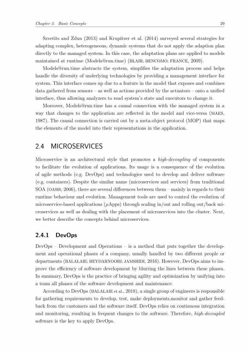
Figure 10 – DevOps operations and some examples of the technologies used in each op-eration.

Source: <www.edureka.co>

To correctly apply the DevOps, it is necessary to automatize the life-cycle phases, asshown in FIG. 10. Test, integration, deployment and monitoring phases are carried outautomatically, allowing engineers to focus on planning and coding the application. Toachieve this high automation degree, it is necessary continually monitor several aspectsof the software. All these data are used as feedback and tools, allowing the engineers toevolve the application fast and continuously.

However, this in-depth monitoring has a cost. The heterogeneity and amount of datacollected eventually overwhelms the DevOps engineer, making it difficult to analyze allthe information generated and plan an optimal strategy to act in response.

2.4.2 Containers

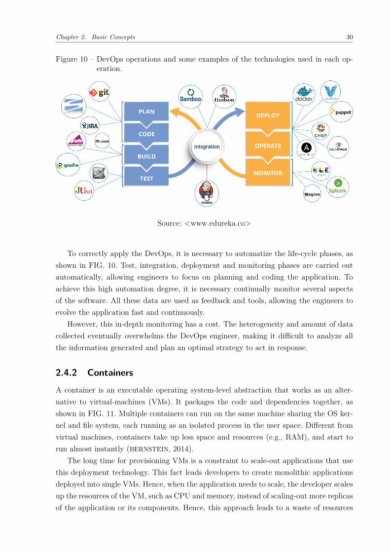
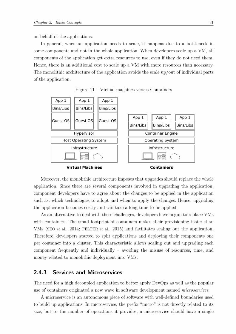
A container is an executable operating system-level abstraction that works as an alter-native to virtual-machines (VMs). It packages the code and dependencies together, asshown in FIG. 11. Multiple containers can run on the same machine sharing the OS ker-nel and file system, each running as an isolated process in the user space. Different fromvirtual machines, containers take up less space and resources (e.g., RAM), and start torun almost instantly (BERNSTEIN, 2014).

The long time for provisioning VMs is a constraint to scale-out applications that usethis deployment technology. This fact leads developers to create monolithic applicationsdeployed into single VMs. Hence, when the application needs to scale, the developer scalesup the resources of the VM, such as CPU and memory, instead of scaling-out more replicasof the application or its components. Hence, this approach leads to a waste of resources

Chapter 2. Basic Concepts 31

on behalf of the applications.In general, when an application needs to scale, it happens due to a bottleneck in

some components and not in the whole application. When developers scale up a VM, allcomponents of the application get extra resources to use, even if they do not need them.Hence, there is an additional cost to scale up a VM with more resources than necessary.The monolithic architecture of the application avoids the scale up/out of individual partsof the application.

Figure 11 – Virtual machines versus Containers

Moreover, the monolithic architecture imposes that upgrades should replace the wholeapplication. Since there are several components involved in upgrading the application,component developers have to agree about the changes to be applied in the applicationsuch as: which technologies to adopt and when to apply the changes. Hence, upgradingthe application becomes costly and can take a long time to be applied.

As an alternative to deal with these challenges, developers have begun to replace VMswith containers. The small footprint of containers makes their provisioning faster thanVMs (SEO et al., 2014; FELTER et al., 2015) and facilitates scaling out the application.Therefore, developers started to split applications and deploying their components oneper container into a cluster. This characteristic allows scaling out and upgrading eachcomponent frequently and individually – avoiding the misuse of resources, time, andmoney related to monolithic deployment into VMs.

2.4.3 Services and Microservices

The need for a high decoupled application to better apply DevOps as well as the popularuse of containers originated a new wave in software development named microservices.

A microservice is an autonomous piece of software with well-defined boundaries usedto build up applications. In microservice, the prefix “micro” is not directly related to itssize, but to the number of operations it provides; a microservice should have a single

Chapter 2. Basic Concepts 32

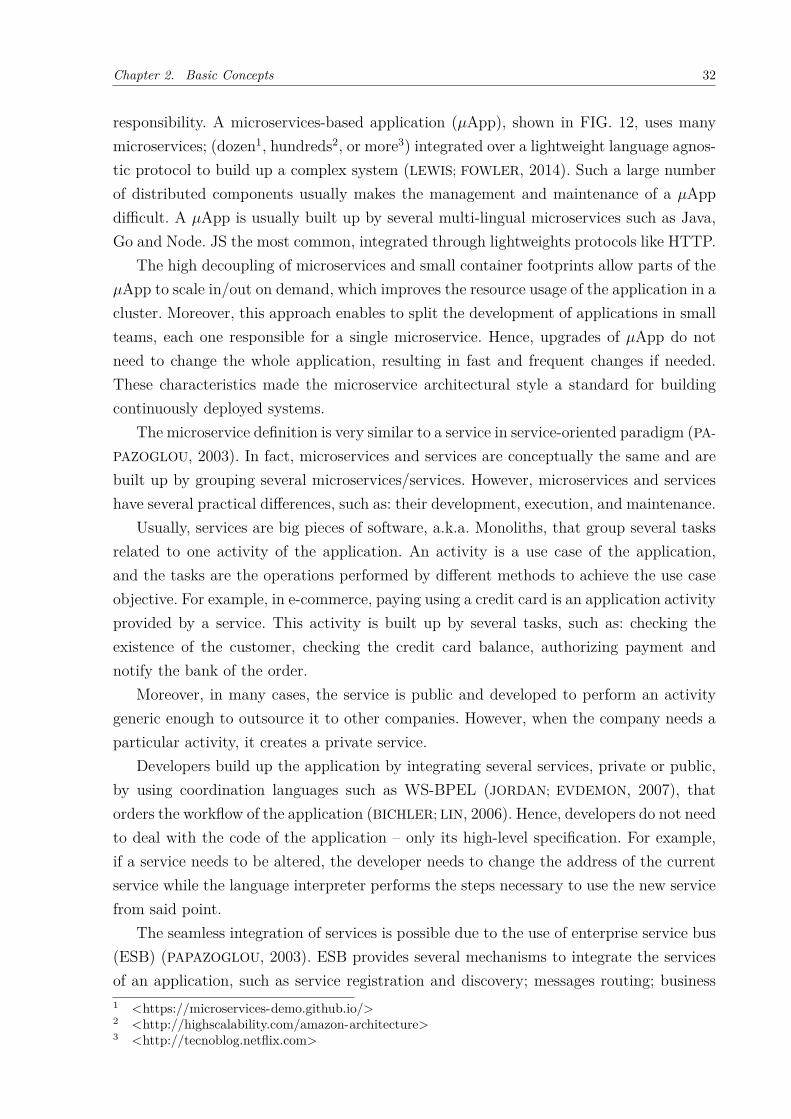
responsibility. A microservices-based application (𝜇App), shown in FIG. 12, uses manymicroservices; (dozen1, hundreds2, or more3) integrated over a lightweight language agnos-tic protocol to build up a complex system (LEWIS; FOWLER, 2014). Such a large numberof distributed components usually makes the management and maintenance of a 𝜇Appdifficult. A 𝜇App is usually built up by several multi-lingual microservices such as Java,Go and Node. JS the most common, integrated through lightweights protocols like HTTP.

The high decoupling of microservices and small container footprints allow parts of the𝜇App to scale in/out on demand, which improves the resource usage of the application in acluster. Moreover, this approach enables to split the development of applications in smallteams, each one responsible for a single microservice. Hence, upgrades of 𝜇App do notneed to change the whole application, resulting in fast and frequent changes if needed.These characteristics made the microservice architectural style a standard for buildingcontinuously deployed systems.

The microservice definition is very similar to a service in service-oriented paradigm (PA-

PAZOGLOU, 2003). In fact, microservices and services are conceptually the same and arebuilt up by grouping several microservices/services. However, microservices and serviceshave several practical differences, such as: their development, execution, and maintenance.

Usually, services are big pieces of software, a.k.a. Monoliths, that group several tasksrelated to one activity of the application. An activity is a use case of the application,and the tasks are the operations performed by different methods to achieve the use caseobjective. For example, in e-commerce, paying using a credit card is an application activityprovided by a service. This activity is built up by several tasks, such as: checking theexistence of the customer, checking the credit card balance, authorizing payment andnotify the bank of the order.

Moreover, in many cases, the service is public and developed to perform an activitygeneric enough to outsource it to other companies. However, when the company needs aparticular activity, it creates a private service.

Developers build up the application by integrating several services, private or public,by using coordination languages such as WS-BPEL (JORDAN; EVDEMON, 2007), thatorders the workflow of the application (BICHLER; LIN, 2006). Hence, developers do not needto deal with the code of the application – only its high-level specification. For example,if a service needs to be altered, the developer needs to change the address of the currentservice while the language interpreter performs the steps necessary to use the new servicefrom said point.

The seamless integration of services is possible due to the use of enterprise service bus(ESB) (PAPAZOGLOU, 2003). ESB provides several mechanisms to integrate the servicesof an application, such as service registration and discovery; messages routing; business1 <https://microservices-demo.github.io/>2 <http://highscalability.com/amazon-architecture>3 <http://tecnoblog.netflix.com>

Chapter 2. Basic Concepts 33

Figure 12 – Example of 𝜇App.

Source: <https://microservices-demo.github.io/>

rules; messages filtering; service fail-over; message transformations; security and manyothers. This approach forces the application to rely on a single component (single pointof failure) in the application architecture which can threaten the application execution ifit is not working correctly. However, service engineers are free on not to concern aboutseveral non-functional requirements during a service development.

On the other hand, microservices are small pieces of software that provide singleand well-defined functionalities. Unlike services, a microservice does not implement anactivity by itself, but rather a group of microservices each provide a task. Given thecredit card example mentioned before, the activity of processing a payment is made byseveral microservices each one providing a single task.

The integration of microservices relies on the concept of smart endpoints and dumppipes (LEWIS; FOWLER, 2014). The microservice (smart endpoints) receives a request andapplies a logic as an appropriate answer to produce a response. To reach it, the applicationuses simple built-in RESTis protocols rather than WS-BPEL. The microservice itself isresponsible for choreographing the 𝜇App’s behaviour. The integration of microservices isachieved over a lightweight message bus (dump pipes) – RabbitMQ4 or ZeroMQ5 – thatdoes not do much more than provide a reliable mesh connecting the endpoints by routingraw messages without any manipulation.

Moreover, microservices have some degree of autonomy and are implemented by know-ing how to locate and communicate with other microservices. This characteristic meansthat changes in the 𝜇App’s workflow are made by replacing microservices with new ver-sions. In reality, the low coupling between microservices allows them to be changed without4 <https://www.rabbitmq.com/>5 <http://zeromq.org/>

Chapter 2. Basic Concepts 34

affecting others.Ideally, microservices should be stateless. Stateful microservices decrease the flexibility

of 𝜇Apps, locking their placement to data location. Furthermore, microservice manage-ment tools do not have mechanisms to deal with data migration and data replicationwhen scaling in/out microservices or new microservice version deployment. To avoid datalocking, 𝜇Apps regularly use data stores provided by cloud providers, such as AmazonSimple Storage Service6, instead of managing their data store.

2.4.4 Microservices Management Tools

The high coupling between microservices and containers has led to the use of singlemanagement tools to control container’s life-cycle and microservices. Cloud Foundry7,Docker Swarm8 and Kubernetes9 are widely used to manage containers, and consequentlymicroservices (BERNSTEIN, 2014).

The management tools do not handle microservices directly, in fact the microservicesmust be wrapped into containers or other technology specific abstraction, e.g, Pods inKubernetes. Along to this document we assume that all microservices are individuallywrapped as required by the management tool, so that microservices and containers (orPods) can be used interchangeable in this document. It is worth observing that Kubernetesis by far the most popular, being the management tool made available by cloud providerssuch as Google, Microsoft and Amazon.

Management tools are responsible for dealing with auto-scaling and deployment ofmicroservices, as well as providing registering and discovering services and some securityto 𝜇App developers. Management tools collect instantaneous information off microser-vice execution – resource usage and microservices logs (BERNSTEIN, 2014). However, be-havioural information such as message exchanges and resource history is not provided bymanagement tools. Despite some automation, application developers are responsible formicroservice management, such as defining the number of replicas and triggering scalein/out actions.

When an engineer configures a microservice to be deployed, some parameters usedby the management tool at runtime are set. In general, engineers set the max and minamount of resources required by the microservice, max and min number of replicas avail-able at runtime, and thresholds used to trigger scaling in/out and to request/releasehost resources. At runtime, management tools collect instantaneous snapshots of resourceusage and compare them with the values set by engineers,scaling the microservice orrequesting/releasing resources.6 <https://aws.amazon.com/documentation/s3/>7 <https://www.cloudfoundry.org/>8 <https://docs.docker.com/swarm/overview/>9 <https://kubernetes.io>

Chapter 2. Basic Concepts 35

In addition to the mentioned limits and thresholds, management tools allow microser-vices to be tagged. These tags can be used at runtime to map microservices to specifichosts according to annotations in the microservice and hosts. Moreover, management toolsprovide these tags at runtime through API for third-party tools to use.

2.4.5 𝜇Apps Architectures

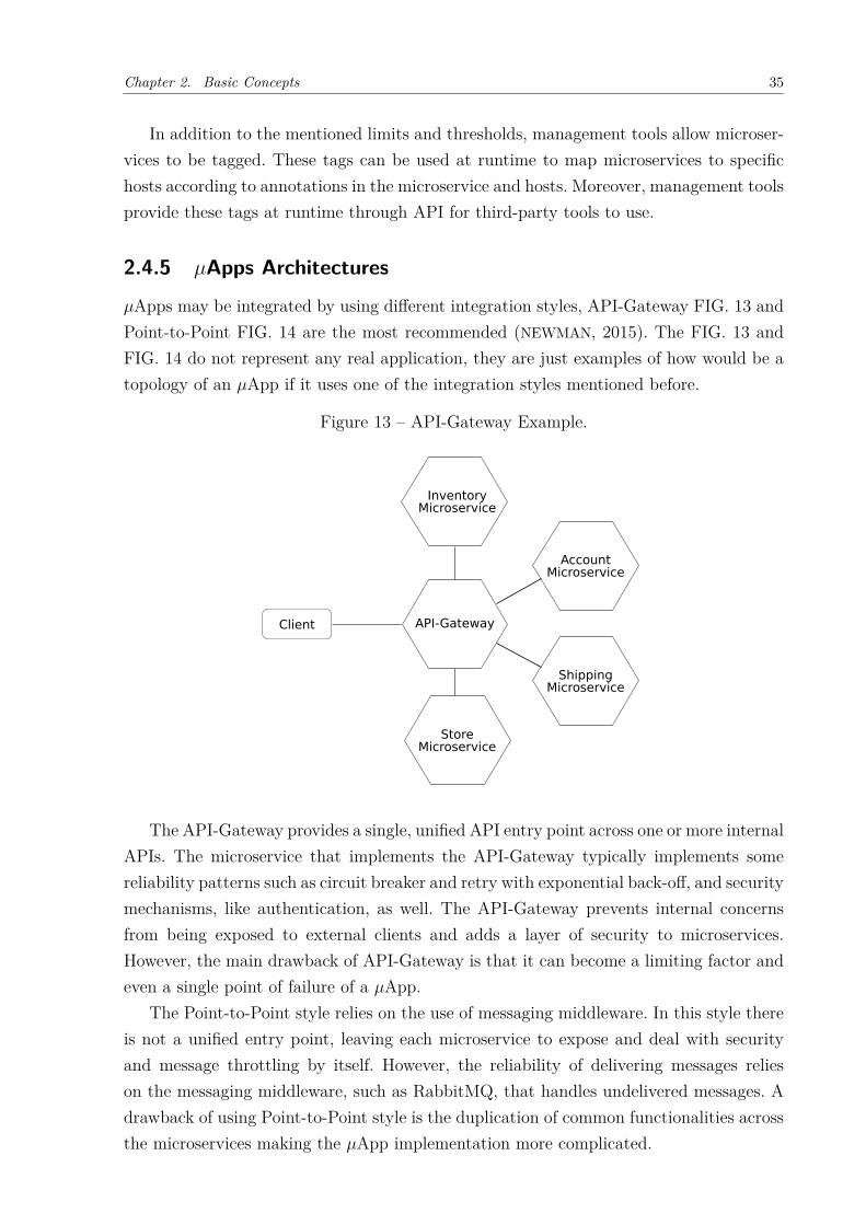
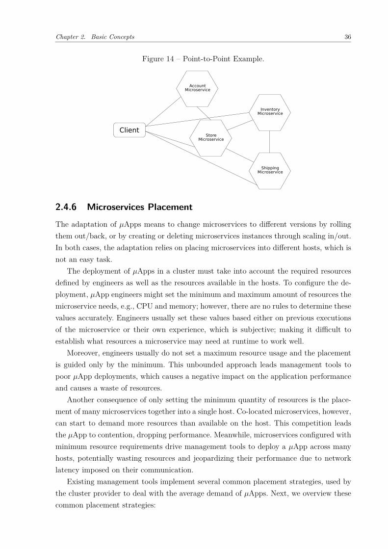
𝜇Apps may be integrated by using different integration styles, API-Gateway FIG. 13 andPoint-to-Point FIG. 14 are the most recommended (NEWMAN, 2015). The FIG. 13 andFIG. 14 do not represent any real application, they are just examples of how would be atopology of an 𝜇App if it uses one of the integration styles mentioned before.

Figure 13 – API-Gateway Example.

InventoryMicroservice

Client API-Gateway

StoreMicroservice

AccountMicroservice

ShippingMicroservice

The API-Gateway provides a single, unified API entry point across one or more internalAPIs. The microservice that implements the API-Gateway typically implements somereliability patterns such as circuit breaker and retry with exponential back-off, and securitymechanisms, like authentication, as well. The API-Gateway prevents internal concernsfrom being exposed to external clients and adds a layer of security to microservices.However, the main drawback of API-Gateway is that it can become a limiting factor andeven a single point of failure of a 𝜇App.

The Point-to-Point style relies on the use of messaging middleware. In this style thereis not a unified entry point, leaving each microservice to expose and deal with securityand message throttling by itself. However, the reliability of delivering messages relieson the messaging middleware, such as RabbitMQ, that handles undelivered messages. Adrawback of using Point-to-Point style is the duplication of common functionalities acrossthe microservices making the 𝜇App implementation more complicated.

Chapter 2. Basic Concepts 36

Figure 14 – Point-to-Point Example.

2.4.6 Microservices Placement

The adaptation of 𝜇Apps means to change microservices to different versions by rollingthem out/back, or by creating or deleting microservices instances through scaling in/out.In both cases, the adaptation relies on placing microservices into different hosts, which isnot an easy task.

The deployment of 𝜇Apps in a cluster must take into account the required resourcesdefined by engineers as well as the resources available in the hosts. To configure the de-ployment, 𝜇App engineers might set the minimum and maximum amount of resources themicroservice needs, e.g., CPU and memory; however, there are no rules to determine thesevalues accurately. Engineers usually set these values based either on previous executionsof the microservice or their own experience, which is subjective; making it difficult toestablish what resources a microservice may need at runtime to work well.

Moreover, engineers usually do not set a maximum resource usage and the placementis guided only by the minimum. This unbounded approach leads management tools topoor 𝜇App deployments, which causes a negative impact on the application performanceand causes a waste of resources.

Another consequence of only setting the minimum quantity of resources is the place-ment of many microservices together into a single host. Co-located microservices, however,can start to demand more resources than available on the host. This competition leadsthe 𝜇App to contention, dropping performance. Meanwhile, microservices configured withminimum resource requirements drive management tools to deploy a 𝜇App across manyhosts, potentially wasting resources and jeopardizing their performance due to networklatency imposed on their communication.

Existing management tools implement several common placement strategies, used bythe cluster provider to deal with the average demand of 𝜇Apps. Next, we overview thesecommon placement strategies:

Chapter 2. Basic Concepts 37

Spread strategy. The management tool places a minimum number of microservicesper host in the cluster. This strategy tries to avoid resource contention since fewconcurrent microservices will dispute the same resources. However, it can lower𝜇App performance by adding latency to request/response messages as microservicesmay be deployed on different hosts. Moreover, this strategy can waste resources sincesome microservices may need fewer resources than what their host provides. DockerSwarm and Kubernetes adopt the spread strategy.

Bin-pack strategy. The management tool uses the minimum number of hosts to de-ploy a 𝜇App, avoiding cluster resource waste. However, putting many microservicestogether causes contention for the same resources, dropping 𝜇App performance dras-tically. This strategy is available in Docker Swarm.

Labeled strategy. In addition to the resource requirements, microservices can be taggedwith attributes used to guide host selection. For example, a machine learning 𝜇Appcan require being deployed on hosts with GPUs for performance reasons. Then, atdeployment time, the management tool selects a host that matches the microser-vice labelled requirements. This strategy is usually used to customize the defaultmanagement tool strategy. For example, the default strategy of Docker Swarm andKubernetes can be customized with labels as constraints on the placement of somemicroservices.

Random strategy. The management tool selects a host to deploy a microservice ran-domly. This strategy is available in Docker Swarm.

Finally, most of management tools provide abstractions to force microservices to beco-located during the deployment. However, this abstractions are static, they cannotchange automatically at runtime according to variations of the 𝜇App behavior. Thisco-locations should be set by the engineers that, not necessarily, have all informationneeded to set them usefully.

2.5 CONCLUDING REMARKSIn this chapter, we initially presented the central concepts of autonomous computingand adaptive systems focusing on MAPE-K architecture. We showed the consequencesof using different deployment configuration to deploy MAPE-K. We also presented thenotion of model and Models@run.time, and how Models@run.time can be used on adaptivesystems. Finally, we presented the primary motivations behind microservices along witha discussion about the differences to the traditional idea of service in service-orientedcomputing.

38

3 REMAP - RATIONALE AND GENERALOVERVIEW

In this chapter, we present the challenges of evolving 𝜇Apps at runtime and highlightthe critical challenges of adapting 𝜇Apps at runtime. We highlight the monitoring andplacement of microservices on a cluster as the critical challenges to be handled in adapting𝜇Apps. Next, we present an overview of our proposal to perform runtime adaptation on𝜇Apps. Moreover, we describe the concept of model evolution and how it is used to guidethe adaptation of 𝜇Apps. Finally, we characterize the problem microservice placement atruntime and how it affects the 𝜇Apps.

3.1 CHALLENGES ON RUNTIME EVOLUTION OF 𝜇APPSThe decoupling promoted by the Microservice architectural style facilitates applyingchanges to the 𝜇App– allowing engineers to replace or scale microservices without collat-eral effects on the application structure. Engineers do not need to halt the application toapply change. Therefore, we define 𝜇Apps as an inherited adaptive application.

However, high decoupling in 𝜇Apps is a two-sided sword for their maintenance. On onehand, decoupling allows engineers fixing the 𝜇App or adopt new technologies smoothly. Onthe other hand, this ease in changing microservices may threat the application’s behaviourif applied in a careless fashion – when engineers take into consideration the past behaviourof the 𝜇App (e.g., its workflow or resource usage), the adaptation may lead the to a poorperformance on behalf of the 𝜇App.

Changes on 𝜇Apps rely basically on Microservice placement. Hence, in order to decidewhen and why to change the 𝜇App, it is necessary to observe different aspects of theapplication. However, due to the heterogeneity of 𝜇Apps, monitoring is not a simple task.Furthermore, the dynamics of a 𝜇App can affect or be affected according to where themicroservices are placed. Next, we expand the discussion of the challenges in monitoringand placing microservices at runtime.

3.1.1 Challenges in Monitoring

Despite the microservice style facilitating how the changes in 𝜇Apps occur, it makes itdifficult to identify what and when it is necessary to adapt the application. Hence, it isessential to observe the behaviour of the 𝜇App.

The behaviour of a black-box 𝜇App can be observed in at least three ways:

Chapter 3. REMaP - Rationale and General Overview 39

Resource usage The resource usage is the amount of resource used by a microservicewhile the 𝜇App executes – CPU, memory, disk and network bandwidth.

Application logs 𝜇App engineers determine application events to signal errors, warn-ings and informational messages throughout its execution. Informational messagesdo not log warnings or errors, but it informs what is happening throughout theapplication execution (e.g."[INFO] loading library xxx"). Dedicated tools maintainthe events in the sequence they occur and allow the engineers to use the applicationlogs for tracking the 𝜇App execution.

Message information Messages exchanged by microservices, including: message sourcesand destinations; payload size; some metrics, such as response time; and contextualdata, such as HTTP headers and response codes.

Due to the large number of microservices in a 𝜇App– different types of microservicesand their replicas building up the 𝜇App– its execution generates a huge amount of hetero-geneous data, which makes it challenging to monitor the 𝜇App. To make matters worse,the diversity of technologies used in the microservice domain makes it difficult to get aunified view of the 𝜇App at runtime.

A 𝜇App is potentially multi-lingual and multi-technological, which means that varioustools are necessary to monitor the same information across different microservices in the𝜇App. The broad diversity of tools to collect data and track 𝜇App behaviour is madeworse by the fact that, in general, existing tools do not follow any standard. This lack ofstandard creates a semantic gap in the provided information. For example, data metricscollected by Influxdb1 and Prometheus2 have different formats. Therefore, it is difficultto observe the dynamics of 𝜇Apps running on the same cluster, since each one can use adifferent monitoring stack.

Furthermore, not all languages include bindings for a specific tool, e.g., Zipkin3, whichmeans that different tools may monitor microservices belonging to the same 𝜇App. Theheterogeneity of monitoring tools is a challenge as there is a need to deal with differentsemantics, data structures and technologies.

Although monitoring tools can collect information from a 𝜇App execution (e.g., instan-taneous resource usage), they are unable to collect behavioural aspects such as resourceusage history and 𝜇App workflow. Instantaneous data alone is not enough to track the be-haviour of a 𝜇App– maintaining historical data along the execution is essential. Nowadays,engineers use third-party tools to record and track historical data of 𝜇Apps, since man-agement tools only expose instantaneous microservice information. Some existing toolsare now being used for this purpose: cAdvisor4 gathers cluster (hosts) and microservices1 <https://www.influxdata.com/>2 <https://prometheus.io/>3 <https://zipkin.io>4 <https://github.com/google/cadvisor>

Chapter 3. REMaP - Rationale and General Overview 40

(wrapped into containers) metrics natively; Prometheus stores data collected by cAdvisoror self-stored by microservices; and Influxdb stores monitored data.

Moreover, none of the current management tools are aware of messages exchangedbetween microservices. This fact is a major drawback since messages are critical to under-standing how a 𝜇App actually works. There are few initiatives to gather and store 𝜇Appsmessages, such as Zipkin5 and Jaeger6.

Despite the fact that management tools expose microservices’ execution logs, thesetools cannot aggregate and use them at runtime. As a result, aggregators are needed inorder to organize logs as well as ensure their temporal order and store them to maintaintheir history. Popular log aggregators include Fluentd7 and Logstash8. It is also necessaryto use data stores like Elasticsearch9 and Influxdb, to maintain a history of the 𝜇Appexecution. Furthermore, cloud providers habitually provide their own private solutionssuch as Amazon CloudWatch10.

Hence, to monitor 𝜇Apps and track their behaviour at runtime, it is necessary touse several tools to gather signals of different aspects of 𝜇App behaviours such as themicroservices’ resource usage and data workflow.

By having all this information, engineers or management tools can understand howthe application works and then compute plans to improve its behaviour. Furthermore, itis possible to use this information as input for an artificial intelligence mechanism whichanticipates future behavior based on past information and applies preemptive adaptationson the system.

Engineers are currently manually analyzing the collected data – retrieving, parsing andsending them to visualization tools (e.g., Kibana11) – and taking action based on what isobserved. These steps make the management of 𝜇Apps complex and error-prone (WARD;

BARKER, 2014).As a consequence, the use of autonomous tools is made necessary in order to improve

𝜇App adaptation, releasing engineers from decision making, makes the whole processfaster and more reliable. However, the challenges in adapting 𝜇Apps are not restrictedto monitoring them – it relies on placing microservices somewhere. Next, we discuss thedetails of this challenge.

3.1.2 Challenges in Placement

The high decoupling provided by microservices facilitates the scaling and upgrading of𝜇Apps, promoting their evolution. In our context, the evolution of 𝜇Apps consists of its5 <https://zipkin.io>6 <https://uber.github.io/jaeger>7 <https://www.fluentd.org>8 <https://www.elastic.co/products/logstash>9 <https://www.elastic.co/products/elasticsearch>10 <https://aws.amazon.com/cloudwatch>11 <https://www.elastic.com/products/kibana>

Chapter 3. REMaP - Rationale and General Overview 41

adaptation by (1) replacing one microservice instance with another, usually on a differenthost, or (2) creating new microservice replicas. Management tools execute such adapta-tions. Hence, we classify 𝜇App adaptation in two types:

1. Updates: The microservice implementation do not change, only their instances arereconfigured, e.g., scaling in/out;

2. Upgrades: The microservice implementation and/or application structure change,e.g., rolling out/back a microservice version.

The evolution of 𝜇Apps is a natural activity in the microservices domain, and asmentioned in Section 2.4, it is the only way to alter the workflow of the 𝜇Apps. Hence,engineers use management tools to carry out the adaptation.

These tools are currently unaware of microservice runtime behaviour, and the decisionto place a microservice somewhere is based exclusively on static values set by engineers.In most cases, these values do not reflect the real behaviour of the 𝜇App, resulting in apoor placement.

For example, a tool can automatically trigger the auto-scaling, but an engineer mustfix both the maximum number of replicas as well as the resource usage that triggers thescaling. In an autonomic approach, the adaptation mechanism would automatically decidethese parameters.

In another example, a new version of microservice "A" has a higher communicationdemand with microservice "B" than in its prior version. The management tool is unawareof 𝜇App communication requirements – it knows nothing about messages exchanged be-tween microservices. Hence, it put these microservices in different places. However, thehigh communication between the two services over the network can hurt the overall per-formance due to network latency. In this case, it would be better to co-locate these bothmicroservices in the same host.

The evolution of 𝜇Apps eventually changes the requirements of their microservices.For example, the upgrade of the 𝜇App either makes some microservices require more orfewer resources at runtime, or breaks or adds relationships between microservices whichchange the workflow of the application.

The management tool, which controls the microservices inside the cluster, shoulddecide where to place the microservices as a consequence of the adaptation. Differentmanagement tools each have their strategy to place microservices but none of them con-sider runtime and history data to make a placement decision. Due to the amount of datagenerated by the 𝜇Apps and its heterogeneity, the management tools discard the pastresource usage and not considers the microservices interactions during its execution. Usu-ally, these tools only consider the current resource usage in order to decide where to placethe microservice after the adaptation.

Chapter 3. REMaP - Rationale and General Overview 42

Nevertheless, the ease of change in microservices can threaten the 𝜇App. The carelessplacement of microservices can lead the application to get undesired behaviours such asresource contention or communication latency.

Resource contention arises when microservices with high resource usage are placedtogether into a cluster node. Due to the lack of information about past resource usageby the microservice, the management tool may place microservices with high resourceusages together. These tools are only aware of the instantaneous state of the applica-tions; therefore it cannot infer any information about past microservice behaviour. Twomicroservices could, for example, have a high resource usage in the morning but low onein the afternoon. If an adaptation is made in the afternoon, the management tool mayplace both together causing the 𝜇App to drop its performance the next morning due toboth microservices competing for resources in their host.

Similarly, the lack of information about the workflow of a 𝜇App endangers its ex-ecution. Management tools are not aware of the 𝜇App’s workflow – all the messagesexchanged by microservices are transparent to the tool. Hence, tools can place high re-lated microservices separated into different hosts, which lowers the 𝜇App’s performancedue to the network latency between the microservices.

However, dealing with placement is not easy. Placing a microservice in a cluster basedon different constraints is an NP-Hard optimization problem. This characteristic makes itdifficult (impossible in some cases) to optimize 𝜇App placement at runtime. It is not easyto have a complete view of the 𝜇Apps in order to decide when to change the application.Therefore, in this thesis, we deal with monitoring and 𝜇App placement problems byproposing REMaP (RuntimE Microservices Placement), an adaptation mechanism toimprove the placement of 𝜇Apps based on its runtime behaviour, past resource usage andits data workflow.

Management tools should be aware of runtime information in 𝜇Apps to avoid the afore-mentioned drawbacks, however they are not. Therefore, we propose the use of REMaP,which uses runtime data to improve microservice placement. The use of runtime data canmake better 𝜇App placement by providing information about different features, such asthe actual resource usage and message exchange.

Next sections present an overview of REMaP, the use of models to support 𝜇Appsevolution, and how to deal with microservices placement at runtime.

3.2 PROPOSED SOLUTION - OVERVIEWREMaP (RuntimE Microservices Placement) is an autonomous mechanism for adapting𝜇Apps in a cluster at runtime whose architecture, shown in FIG. 15, is based on MAPE-Kand was designed to handle seveal 𝜇Apps in a cluster. REMaP automatizes the adaptationof 𝜇Apps and improves their placement. The proposed solution uses Models@run.time

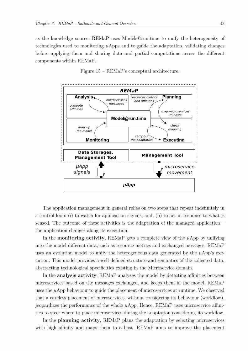
Chapter 3. REMaP - Rationale and General Overview 43

as the knowledge source. REMaP uses Models@run.time to unify the heterogeneity oftechnologies used to monitoring 𝜇Apps and to guide the adaptation, validating changesbefore applying them and sharing data and partial computations across the differentcomponents within REMaP.

Figure 15 – REMaP’s conceptual architecture.

The application management in general relies on two steps that repeat indefinitely ina control-loop: (i) to watch for application signals; and, (ii) to act in response to what issensed. The outcome of these activities is the adaptation of the managed application –the application changes along its execution.

In the monitoring activity, REMaP gets a complete view of the 𝜇App by unifyinginto the model different data, such as resource metrics and exchanged messages. REMaPuses an evolution model to unify the heterogeneous data generated by the 𝜇App’s exe-cution. This model provides a well-defined structure and semantics of the collected data,abstracting technological specificities existing in the Microservice domain.

In the analysis activity, REMaP analyzes the model by detecting affinities betweenmicroservices based on the messages exchanged, and keeps them in the model. REMaPuses the 𝜇App behaviour to guide the placement of microservices at runtime. We observedthat a careless placement of microservices, without considering its behaviour (workflow),jeopardizes the performance of the whole 𝜇App. Hence, REMaP uses microservice affini-ties to steer where to place microservices during the adaptation considering its workflow.

In the planning activity, REMaP plans the adaptation by selecting microserviceswith high affinity and maps them to a host. REMaP aims to improve the placement

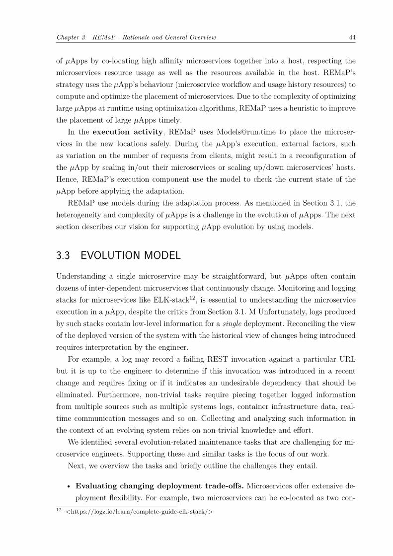
Chapter 3. REMaP - Rationale and General Overview 44

of 𝜇Apps by co-locating high affinity microservices together into a host, respecting themicroservices resource usage as well as the resources available in the host. REMaP’sstrategy uses the 𝜇App’s behaviour (microservice workflow and usage history resources) tocompute and optimize the placement of microservices. Due to the complexity of optimizinglarge 𝜇Apps at runtime using optimization algorithms, REMaP uses a heuristic to improvethe placement of large 𝜇Apps timely.

In the execution activity, REMaP uses Models@run.time to place the microser-vices in the new locations safely. During the 𝜇App’s execution, external factors, suchas variation on the number of requests from clients, might result in a reconfiguration ofthe 𝜇App by scaling in/out their microservices or scaling up/down microservices’ hosts.Hence, REMaP’s execution component use the model to check the current state of the𝜇App before applying the adaptation.

REMaP use models during the adaptation process. As mentioned in Section 3.1, theheterogeneity and complexity of 𝜇Apps is a challenge in the evolution of 𝜇Apps. The nextsection describes our vision for supporting 𝜇App evolution by using models.

3.3 EVOLUTION MODELUnderstanding a single microservice may be straightforward, but 𝜇Apps often containdozens of inter-dependent microservices that continuously change. Monitoring and loggingstacks for microservices like ELK-stack12, is essential to understanding the microserviceexecution in a 𝜇App, despite the critics from Section 3.1. M Unfortunately, logs producedby such stacks contain low-level information for a single deployment. Reconciling the viewof the deployed version of the system with the historical view of changes being introducedrequires interpretation by the engineer.

For example, a log may record a failing REST invocation against a particular URLbut it is up to the engineer to determine if this invocation was introduced in a recentchange and requires fixing or if it indicates an undesirable dependency that should beeliminated. Furthermore, non-trivial tasks require piecing together logged informationfrom multiple sources such as multiple systems logs, container infrastructure data, real-time communication messages and so on. Collecting and analyzing such information inthe context of an evolving system relies on non-trivial knowledge and effort.

We identified several evolution-related maintenance tasks that are challenging for mi-croservice engineers. Supporting these and similar tasks is the focus of our work.

Next, we overview the tasks and briefly outline the challenges they entail.

• Evaluating changing deployment trade-offs. Microservices offer extensive de-ployment flexibility. For example, two microservices can be co-located as two con-

12 <https://logz.io/learn/complete-guide-elk-stack/>

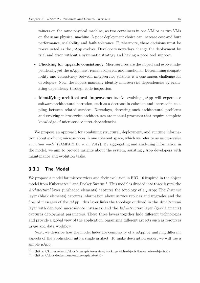
Chapter 3. REMaP - Rationale and General Overview 45

tainers on the same physical machine, as two containers in one VM or as two VMson the same physical machine. A poor deployment choice can increase cost and hurtperformance, scalability and fault tolerance. Furthermore, these decisions must bere-evaluated as the 𝜇App evolves. Developers nowadays change the deployment bytrial and error without a systematic strategy and having a poor tool support.

• Checking for upgrade consistency. Microservices are developed and evolve inde-pendently, yet the 𝜇App must remain coherent and functional. Determining compat-ibility and consistency between microservice versions is a continuous challenge fordevelopers. Now, developers manually identify microservice dependencies by evalu-ating dependency through code inspection.

• Identifying architectural improvements. An evolving 𝜇App will experiencesoftware architectural corrosion, such as a decrease in cohesion and increase in cou-pling between related services. Nowadays, detecting such architectural problemsand evolving microservice architectures are manual processes that require completeknowledge of microservice inter-dependencies.

We propose an approach for combining structural, deployment, and runtime informa-tion about evolving microservices in one coherent space, which we refer to as microserviceevolution model (SAMPAIO JR. et al., 2017). By aggregating and analyzing information inthe model, we aim to provide insights about the system, assisting 𝜇App developers withmaintenance and evolution tasks.

3.3.1 The Model

We propose a model for microservices and their evolution in FIG. 16 inspired in the objectmodel from Kubernetes13 and Docker Swarm14. This model is divided into three layers: theArchitectural layer (unshaded elements) captures the topology of a 𝜇App; The Instancelayer (black elements) captures information about service replicas and upgrades and theflow of messages of the 𝜇App– this layer links the topology outlined in the Architecturallayer with deployed microservice instances; and the Infrastructure layer (gray elements)captures deployment parameters. These three layers together hide different technologiesand provide a global view of the application, organizing different aspects such as resourcesusage and data workflow.

Next, we describe how the model hides the complexity of a 𝜇App by unifying differentaspects of the application into a single artifact. To make description easier, we will use asimple 𝜇App.13 <https://kubernetes.io/docs/concepts/overview/working-with-objects/kubernetes-objects/>14 <https://docs.docker.com/engine/api/latest/>

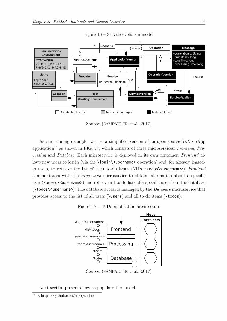
Chapter 3. REMaP - Rationale and General Overview 46

Figure 16 – Service evolution model.

Provider

Application

Scenario

Service

+isExternal: boolean

Message

+correlationId: String+timestamp: long+totalTime: long+processingTime: long

Operation

ServiceVersionServiceReplica

Location Host

+hosting: Environment

*

{ordered}

*

*

*

*

*

*

*

+sourceOperationVersion

+target

ApplicationVersion*

**

*

*

+API*

«enumeration»Environment

CONTAINERVIRTUAL_MACHINEPHYSICAL_MACHINE

Metric

+cpu: float+memory: float

*

*

Architectural Layer Instance LayerInfrastructure Layer

*

*

Source: (SAMPAIO JR. et al., 2017)

As our running example, we use a simplified version of an open-source ToDo 𝜇Appapplication15 as shown in FIG. 17, which consists of three microservices: Frontend, Pro-cessing and Database. Each microservice is deployed in its own container. Frontend al-lows new users to log in (via the \login\<username> operation) and, for already logged-in users, to retrieve the list of their to-do items (\list-todos\<username>). Frontendcommunicates with the Processing microservice to obtain information about a specificuser (\users\<username>) and retrieve all to-do lists of a specific user from the database(\todos\<username>). The database access is managed by the Database microservice thatprovides access to the list of all users (\users) and all to-do items (\todos).

Figure 17 – ToDo application architecture

Frontend

Processing

Database

Containers

Host

\login\<username>

\list-todos

\users\<username>

\todo\<username>

\users

\todos

Source: (SAMPAIO JR. et al., 2017)

Next section presents how to populate the model.15 <https://github.com/h4xr/todo>

Chapter 3. REMaP - Rationale and General Overview 47

3.3.2 Populating the Model

A 𝜇App is represented by element Application in FIG. 16, which consists of a set of Ser-vices, each one exposing a set of Operations. In the example shown in FIG. 17, the Fron-tend service exposes two operations: \login\<username> and \list-todos\<username>.External services are “black-box” services managed by third-party organizations and aremarked using the isExternal flag.

A Scenario describes a high-level use case of the application and is carried out byan ordered list of operations executed by the microservices. In the ToDo application,such scenarios include users logging into the application and retrieving their to-dos. Thelogin scenario is carried out by the Frontend \login\<username> operation followed bythe Processing \users\<username> operation and Database \users operation. A scenariospecifies the allowed order of operations, helping to detect faulty behaviours. For example,there is not a scenario in which the Processing \todo\<username> operation precedes theFrontend \login\<username> operation.

The ServiceVersion and OperationVersion elements keep track of changes in servicesand their interfaces. Any Microservice upgrade creates a new ServiceVersion element. Inaddition, if the upgrade involves an operation change, a new OperationVersion elementis created and attached to the new ServiceVersion element. For example, adding the\create-todo\<todo> operation in the Frontend microservice, as shown in FIG. 18, willcreate new ServiceVersion and Operation instances.

Figure 18 – Two versions of Frontend, differing in their supported operations.

FrontendProcessing Database

Frontend

v1

v2

\login\<username>\list-todos

\login\<username>

\create-todo\<todo>

\list-todos

Source: (SAMPAIO JR. et al., 2017)

In Canary releases16, multiple services and multiple versions of the same service can runin parallel to each other as part of the same application. The ApplicationVersion element,groups all service versions in a particular configuration. A sequence of ApplicationVersionscaptures the evolution of an application over time.

To model scale-in and out of services, multiple identical instances of a service versionare represented by the ServiceReplica element. ServiceReplicas are Hosted by containersor by physical and virtual machines, depending on the Environment made available by thecloud Provider. Cloud providers such as Amazon AWS, Microsoft Azure, IBM Bluemixand Google Cloud Platform offer several hosting environments.16 <https://martinfowler.com/bliki/CanaryRelease.html>

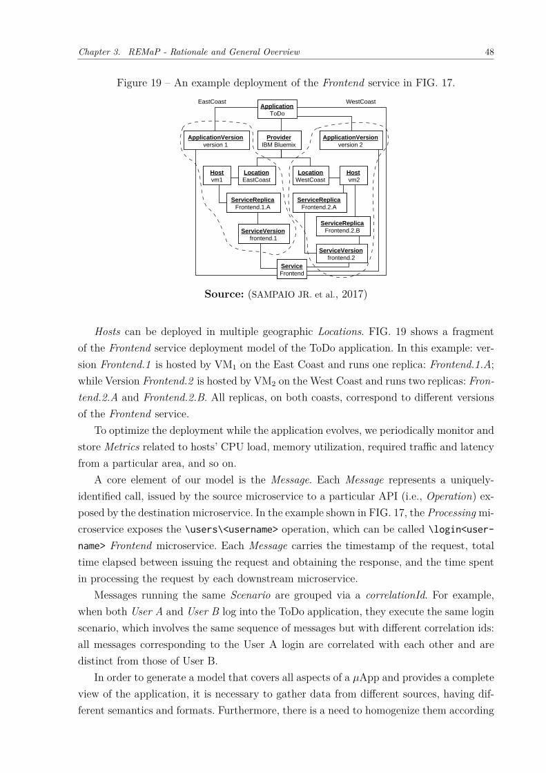
Chapter 3. REMaP - Rationale and General Overview 48

Figure 19 – An example deployment of the Frontend service in FIG. 17.

LocationWestCoast

LocationEastCoast

Hostvm1

Hostvm2

ServiceReplicaFrontend.2.A

ServiceReplicaFrontend.1.A

ServiceReplicaFrontend.2.B

ServiceFrontend

ProviderIBM Bluemix

ServiceVersionfrontend.2

ServiceVersionfrontend.1

ApplicationToDo

ApplicationVersionversion 2

ApplicationVersionversion 1

EastCoast WestCoast

Source: (SAMPAIO JR. et al., 2017)

Hosts can be deployed in multiple geographic Locations. FIG. 19 shows a fragmentof the Frontend service deployment model of the ToDo application. In this example: ver-sion Frontend.1 is hosted by VM1 on the East Coast and runs one replica: Frontend.1.A;while Version Frontend.2 is hosted by VM2 on the West Coast and runs two replicas: Fron-tend.2.A and Frontend.2.B. All replicas, on both coasts, correspond to different versionsof the Frontend service.

To optimize the deployment while the application evolves, we periodically monitor andstore Metrics related to hosts’ CPU load, memory utilization, required traffic and latencyfrom a particular area, and so on.

A core element of our model is the Message. Each Message represents a uniquely-identified call, issued by the source microservice to a particular API (i.e., Operation) ex-posed by the destination microservice. In the example shown in FIG. 17, the Processing mi-croservice exposes the \users\<username> operation, which can be called \login<user-

name> Frontend microservice. Each Message carries the timestamp of the request, totaltime elapsed between issuing the request and obtaining the response, and the time spentin processing the request by each downstream microservice.

Messages running the same Scenario are grouped via a correlationId. For example,when both User A and User B log into the ToDo application, they execute the same loginscenario, which involves the same sequence of messages but with different correlation ids:all messages corresponding to the User A login are correlated with each other and aredistinct from those of User B.

In order to generate a model that covers all aspects of a 𝜇App and provides a completeview of the application, it is necessary to gather data from different sources, having dif-ferent semantics and formats. Furthermore, there is a need to homogenize them according

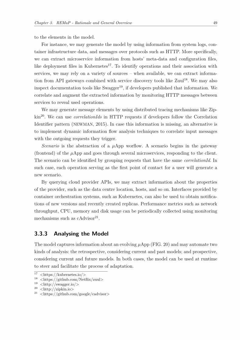
Chapter 3. REMaP - Rationale and General Overview 49

to the elements in the model.For instance, we may generate the model by using information from system logs, con-

tainer infrastructure data, and messages over protocols such as HTTP. More specifically,we can extract microservice information from hosts’ meta-data and configuration files,like deployment files in Kubernetes17. To identify operations and their association withservices, we may rely on a variety of sources – when available, we can extract informa-tion from API gateways combined with service discovery tools like Zuul18. We may alsoinspect documentation tools like Swagger19, if developers published that information. Wecorrelate and augment the extracted information by monitoring HTTP messages betweenservices to reveal used operations.

We may generate message elements by using distributed tracing mechanisms like Zip-kin20. We can use correlationIds in HTTP requests if developers follow the CorrelationIdentifier pattern (NEWMAN, 2015). In case this information is missing, an alternative isto implement dynamic information flow analysis techniques to correlate input messageswith the outgoing requests they trigger.

Scenario is the abstraction of a 𝜇App worflow. A scenario begins in the gateway(frontend) of the 𝜇App and goes through several microservices, responding to the client.The scenario can be identified by grouping requests that have the same correlationId. Insuch case, each operation serving as the first point of contact for a user will generate anew scenario.

By querying cloud provider APIs, we may extract information about the propertiesof the provider, such as the data centre location, hosts, and so on. Interfaces provided bycontainer orchestration systems, such as Kubernetes, can also be used to obtain notifica-tions of new versions and recently created replicas. Performance metrics such as networkthroughput, CPU, memory and disk usage can be periodically collected using monitoringmechanisms such as cAdvisor21.

3.3.3 Analysing the Model

The model captures information about an evolving 𝜇App (FIG. 20) and may automate twokinds of analysis: the retrospective, considering current and past models; and prospective,considering current and future models. In both cases, the model can be used at runtimeto steer and facilitate the process of adaptation.17 <https://kubernetes.io/>18 <https://github.com/Netflix/zuul>19 <http://swagger.io/>20 <http://zipkin.io>21 <https://github.com/google/cadvisor>

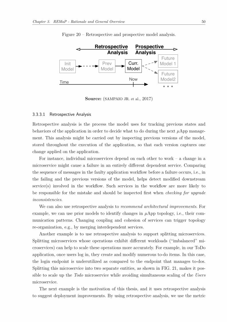
Chapter 3. REMaP - Rationale and General Overview 50

Figure 20 – Retrospective and prospective model analysis.

Curr. Model

Future Model 1… Prev

ModelFuture Model2…Time

Now

RetrospectiveAnalysis

ProspectiveAnalysis

Init Model

Source: (SAMPAIO JR. et al., 2017)

3.3.3.1 Retrospective Analysis

Retrospective analysis is the process the model uses for tracking previous states andbehaviors of the application in order to decide what to do during the next 𝜇App manage-ment. This analysis might be carried out by inspecting previous versions of the model,stored throughout the execution of the application, so that each version captures onechange applied on the application.

For instance, individual microservices depend on each other to work – a change in amicroservice might cause a failure in an entirely different dependent service. Comparingthe sequence of messages in the faulty application workflow before a failure occurs, i.e., inthe failing and the previous versions of the model, helps detect modified downstreamservice(s) involved in the workflow. Such services in the workflow are more likely tobe responsible for the mistake and should be inspected first when checking for upgradeinconsistencies.

We can also use retrospective analysis to recommend architectural improvements. Forexample, we can use prior models to identify changes in 𝜇App topology, i.e., their com-munication patterns. Changing coupling and cohesion of services can trigger topologyre-organization, e.g., by merging interdependent services.

Another example is to use retrospective analysis to support splitting microservices.Splitting microservices whose operations exhibit different workloads (“imbalanced” mi-croservices) can help to scale these operations more accurately. For example, in our ToDoapplication, once users log in, they create and modify numerous to-do items. In this case,the login endpoint is underutilized as compared to the endpoint that manages to-dos.Splitting this microservice into two separate entities, as shown in FIG. 21, makes it pos-sible to scale up the Todo microservice while avoiding simultaneous scaling of the Usersmicroservice.

The next example is the motivation of this thesis, and it uses retrospective analysisto suggest deployment improvements. By using retrospective analysis, we use the metric

Chapter 3. REMaP - Rationale and General Overview 51

history stored in the model, correlated with microservice information such as the inter-action with other microservices and their locations, to suggest deployment improvements.For example, the Frontend and Todo microservices in FIG. 21 are tightly-coupled – in thiscase, our solution may suggest they be located close to each other. On the other hand, theTodo and User microservices do not need such proximity. Likewise, if we observe a suddendecrease in the number of user logs in a certain geographic location, we can recommendremoving the replica from that location, saving money and resources.

Figure 21 – Refactored ToDo application architecture

Frontend

Todo

Database

Host

User

\login\<username>

\list-todos

\users\<username>

\todo\<username>

\users

\todos

Containers

Source: (SAMPAIO JR. et al., 2017)

3.3.3.2 Prospective Analysis

The prospective analysis uses the model as a “sandbox” for exploring the space of possiblearchitectural and deployment refactorings. Several possible refactorings can be emulatedas new snapshots of the model and evaluate their ability to handle the collected real-life𝜇App scenarios. That is, the model can assess potential improvements by replaying thetraces corresponding to the scenarios from the current model in the new model. If thenew model withstands a battery of tests such as replaying traces of a given time intervalin the new model snapshot, we will issue a recommendation to change/refactor the 𝜇App.

Moreover, as mentioned in Section 3.1.1, the model can be used as input for predictiontools (Artificial Intelligence) in order to foresee 𝜇App behavior based on past behavior,thus anticipating actions to improve 𝜇App performance and reliability.

3.3.4 Models@run.time

According to Blair et al. (BLAIR; BENCOMO; FRANCE, 2009), the use of Models@run.-time simplifies the inspection and adaptation of complex heterogeneous Systems. Hence,considering the heterogeneity of monitoring 𝜇Apps, Models@run.time is an interestingconcept to be applied in the managing these applications.

In addition to the retrospective and prospective analysis mentioned before, there isanother advantage of using models at runtime – to plan out elaborate actions that can be

Chapter 3. REMaP - Rationale and General Overview 52

applied to 𝜇Apps. The model organizes data in such a way that planners (see Section 2.1.1)can readily traverse the model, combining and deriving new information, without facingthe semantic gap that appears when dealing with raw data produced by monitoring tools.

Finally, Models@run.time allows safe changes to be applied to 𝜇Apps. Since the modelhas all the information about its underlying application, it is possible to check the changesapplied to the model before consolidating them. For example, suppose that the adaptionneeds to move a microservice to a new host; in this case it is necessary to check within themodel if the target host has sufficient resources to accommodate the microservice, e.g.,considering its resource usage history. Without such a model this evaluation cannot beperformed quickly.

Despite the use of Models@run.time helping in some aspects of 𝜇App adaptations, itremains a challenge to place microservices while adapting a 𝜇App wisely. As discussedin the Section 3.1, 𝜇App adaptation relies on placing microservices in different locations.The next section presents the importance of the optimal placement of microservices.

3.4 PLACEMENT OF MICROSERVICESAnalyzing the messages exchanged by microservices helps us understand their interactions.Related microservices usually exchange a high number of messages and/or a high amountof data. Combining the number of messages and the amount of data gives us an idea ofthe affinity between microservices. High-affinity microservices, placed in different hosts,can impose performance overload on the 𝜇App due to network latency. Therefore, relatedmicroservices should be placed together.

However, putting high-affinity microservices together is not enough to improve 𝜇Appplacement. It is necessary to consider microservice runtime resource usage as well. Existingmanagement tools do not take into account the resource usage history at runtime in orderto place microservices – it can only observe instantaneous resource usage or the values setat configuration by the engineers. However, these values do not reflect the real behaviourof the microservices. Using this information to place microservice instances, can lead the𝜇App to contention situations.

Microservices can use more or fewer resources in specific workflows along 𝜇App execu-tion. Hence, we can observe peaks and lows in resource usage. If the management tool doesa placement based on observing the peaks, it may place the microservices across severalhosts, wasting resources. On the other hand, if the placement is based on the lows, manymicroservices may be co-located into a host, leading the 𝜇App to a contention behaviour.

Although management tools, like Kubernetes, allow setting upper limits for resourceusage, there is no guarantee that engineers will set these limits. And, if these limitsare set, there are no guarantees that the chosen values are the best for all workloadsduring a 𝜇App execution. Moreover, set limits in the management tools does not make

Chapter 3. REMaP - Rationale and General Overview 53

a microservice stay under the limit, it just tells the kernel when to start to constrainthe microservice and when to kill it. This is most evident in interpreted languages, likeJava (prior version 8)22 and Python23, in which the interpreters cannot handle the limitsset on management tools properly and can crash the 𝜇App when the limits are reached.This unbounded/unreliable approach leads management tools to make poor deployments,which may degrade application performance or crash the entire 𝜇App.

Therefore, it is necessary to balance the relationship between microservices and theirresource usage in order to improve their placement. In Section 3.3, we discuss the use ofModels@run.time in keeping runtime (history) data to be used during placement compu-tation. However, only models are not enough to handle the placement problem.

3.4.1 The Placement Problem

Microservice placement improvement is a hard task. Placing microservices in a cluster is avariation of the bin-packing problem (KORTE; VYGEN, 2006). In the bin-packing problem,objects of different sizes must be packed into a finite number of bins of volume 𝑉 in away that minimizes the number of bins needed. This approach is a combined NP-Hardproblem. In our context, the objects to be packed are the microservices and the bins arethe cluster hosts.

It is worth observing that several 𝜇Apps share a single cluster and each one hasdifferent features and requirements. However, management tools are unaware of microser-vice runtime needs. At deployment time, the cluster provider tries to balance the hosts’resource usage without jeopardizing the 𝜇App’s performance. However, the lack of stan-dardization by engineers in setting microservice resource requirements complicates theirplacement.

Whatever the strategy, management tools do not use runtime information or historydata in order to drive or enhance the placement of microservices. Existing tools select thehosts considering the minimum availability of resources to accommodate the microservice,and rarely the maximum. If these requirements are not set, any host can be a candidateto receive a microservice.

Unlike the classical bin-packing problem, the microservice placement in a cluster can-not consider only one dimension (size of microservice), but N dimensions: (i) the mi-croservices affinities and their resources usage, e.g., (ii) CPU, (iii) memory, (iv) disk, andso on. Therefore, our problem is a multi-dimensional variation of bin-packing (CHEKURI;

KHANNA, 2004) that is exponentially harder to solve.The formal statement of the mi-croservice placement problem, guided by affinities is stated as follows:

Given a set of hosts 𝐻1, 𝐻2, · · · , 𝐻𝑚 and a set of 𝜇Apps 𝑃1, 𝑃2, · · · , where 𝑃𝑖 is a setof 𝑛 microservices 𝑚𝑃𝑖,1, 𝑚𝑃𝑖,2, · · ·𝑚𝑃𝑖,𝑛 linked by the affinity function 𝐴 : 𝑚𝑃𝑖

→ 𝑚𝑃𝑖.

22 <https://jaxenter.com/nobody-puts-java-container-129373>23 <https://stackoverflow.com/questions/36759132/why-does-docker-crash-on-high-memory-usage>

Chapter 3. REMaP - Rationale and General Overview 54

Find an integer number of hosts 𝐻 and a 𝐻-partition 𝐻1 ∪ · · · ∪𝐻𝐵 of the set {1, · · · , 𝑛}such that the ⋃︀ of the multi-attributes microservices 𝑚𝑃𝑖,𝑗 fits on 𝐻𝑘 for all 𝑘 = 1, · · · , 𝐵,𝑖 = 1, · · · , 𝑃 , and 𝑗 = 1, · · · , 𝑛𝑃𝑖

. A solution is optimal if it has minimal 𝐵 and maximumaffinity score for all 𝐻𝑘.

The multi-dimensional bin-packing problem adopted in the cluster domain is wellunderstood (CHRISTENSEN et al., 2016). However, the complexity of computing an optimalresult in a reasonable time for large instances prevents its use at runtime.

There are several approaches surveyed by (CHRISTENSEN et al., 2016; KORTE; VYGEN,2006) to compute this optimization in an offline way. At runtime, the best strategiesare approximations, calculated through heuristics and evolving algorithms to achieve aquasi-optimal solution.

3.4.2 Requirements to handle 𝜇App Placement

To optimally place microservices in a cluster, it is first necessary to know how to movethem at runtime. Not all microservices can be moved into a new placement, e.g., statefuland labelled microservices.

Further, a stateful microservice is a kind of data source used by 𝜇Apps. Usually, 𝜇Appsoutsource their data to dedicated storage services provided by cluster infrastructure, whichare out of the scope of management tools. If the 𝜇App has a data store (e.g., SGBDs andNoSQL databases) and it is moved to a new placement, management tools are unable toseamlessly migrate their data to the new destination, which leads to inconsistencies in thestate of the 𝜇App.

Existing management tools have simple primitives used to move a microservice acrossdifferent hosts. However, due to a limitation in existing operating systems and frame-works, it is not possible to live-migrate processes (microservices) between machines. As aworkaround, the movement of a microservice can be emulated by a three-step sequencebased on the blue-green deployment (CARNEIRO; SCHMELMER, 2016):

1. Instantiate the microservice replica at the new location,

2. Wait for the microservice to become ready, i.e., load its libraries and be able tohandle requests, and

3. Remove the microservice replica from the previous location.

Management tools usually have built-in primitives to help to implement these steps.Moreover, additional mechanisms are necessary to change a 𝜇App safely. For example,while a microservice is being replaced, the new instance can become unavailable for a shorttime. During this time, other microservices may attempt to establish communication andwill fail as the new instance is not ready. To deal with these faults, developers use design

Chapter 3. REMaP - Rationale and General Overview 55

patterns like circuit breaker24 and retry with the exponential back off 25 to minimize theirnegative effect on a 𝜇App.

However, stateful microservices may be a source of flaws during 𝜇App adaptation.When a new microservice must replace an old one, the management tool cannot auto-matically synchronize their data. Therefore, when a stateful microservice is updated, amechanism is necessary to deal with state synchronization. However, this approach is outof the scope of this thesis.

In next chapter, we show how REMaP handles these requirements and the strategiesadopted to place microservices at runtime smartly.

3.5 CONCLUDING REMARKSIn this chapter, we discussed the main aspects of runtime adaptation in 𝜇Apps. Weintroduced the monitoring of 𝜇Apps and the placement of microservices as the mainchallenges in carrying out runtime adaptation on 𝜇Apps. Then, we overviewed REMaPour MAPE-K based adaptation mechanism to carry out runtime adaptation on 𝜇Apps.Finally, we present our approach to handle the challenges of monitoring and placingmicroservices. We show our approach using models to support 𝜇App evolution and wedescribed the placement of microservices as a multi-objective bin-packing problem.

24 <http://microservices.io/patterns/reliability/circuit-breaker.html>25 <https://en.wikipedia.org/wiki/Exponential_backoff>

56

4 REMAP - DESIGN AND IMPLEMENTA-TION

While the previous chapter presented the main challenges of runtime evolution of 𝜇Appsand a general overview of REMaP, this chapter presents the design choices in order todeal with the challenges mentioned before. Furthermore, this chapter details the currentimplementation of REMaP to handle the runtime adaptation of 𝜇Apps by reconfiguringtheir placement at runtime.

4.1 BASIC FACTSREMaP (RuntimE Microservices Placement) is a MAPE-K (IBM, 2005) based adaptationmanager that autonomously adapts 𝜇Apps at runtime. Runtime adaptation requires threemain steps: to monitor the system under management; to make a decision based onmonitored data and to execute an adaptation plan taking into account the decision.FIG. 15 overviews REMaP.

When an individual or a group of microservices are rolled out or rolled back, the Adap-tation Manager starts executing the control loop indefinitely at regular time intervals.

The adaptation starts with the Monitor inspecting the 𝜇App through the MonitoringAdapters. The adapters abstract different monitoring technologies to gather useful data,such as resource usage and microservice interactions (𝜇App workflow).

REMaP takes uniformly collected data and populates the application Model. TheAnalyzer inspects the model looking for interactions between microservices in order tocompute their affinities. The Model stores information about affinities and the Planneraccesses this information.

The Planner uses the affinities and resource usage stored in the model to calculatea new placement plan (adaptation plan) for the microservices. The Adaptation Managerapplies the adaptation to the Model and checks the consistency of changes before consoli-dating them into the running 𝜇App. The Adaptation Manager forwards the changes thatdo not violate the model to the Executor.

In this scenario, adaptation means the optimization of microservice placement. Theoptimization relies on two dimensions: microservice affinities and resource usage history.By considering these dimensions, the Planner computes a deployment plan to reducewasted resources as well as improve application performance and decrease communicationlatency.

Unlike traditional approaches – whose only objective is to minimize the number ofbins used, considering the number of items – the optimization of microservice placement

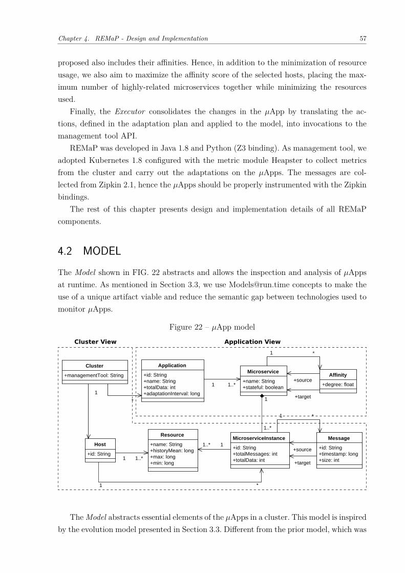
Chapter 4. REMaP - Design and Implementation 57

proposed also includes their affinities. Hence, in addition to the minimization of resourceusage, we also aim to maximize the affinity score of the selected hosts, placing the max-imum number of highly-related microservices together while minimizing the resourcesused.

Finally, the Executor consolidates the changes in the 𝜇App by translating the ac-tions, defined in the adaptation plan and applied to the model, into invocations to themanagement tool API.

REMaP was developed in Java 1.8 and Python (Z3 binding). As management tool, weadopted Kubernetes 1.8 configured with the metric module Heapster to collect metricsfrom the cluster and carry out the adaptations on the 𝜇Apps. The messages are col-lected from Zipkin 2.1, hence the 𝜇Apps should be properly instrumented with the Zipkinbindings.

The rest of this chapter presents design and implementation details of all REMaPcomponents.

4.2 MODELThe Model shown in FIG. 22 abstracts and allows the inspection and analysis of 𝜇Appsat runtime. As mentioned in Section 3.3, we use Models@run.time concepts to make theuse of a unique artifact viable and reduce the semantic gap between technologies used tomonitor 𝜇Apps.

Figure 22 – 𝜇App model

The Model abstracts essential elements of the 𝜇Apps in a cluster. This model is inspiredby the evolution model presented in Section 3.3. Different from the prior model, which was

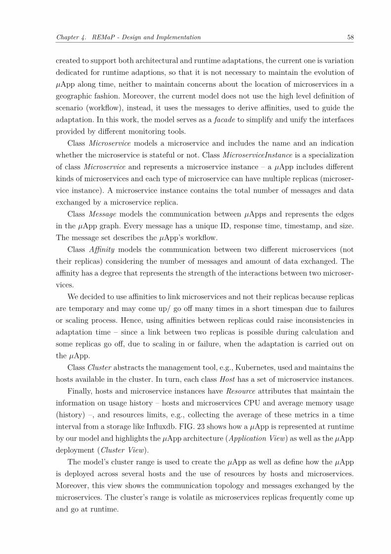
Chapter 4. REMaP - Design and Implementation 58

created to support both architectural and runtime adaptations, the current one is variationdedicated for runtime adaptions, so that it is not necessary to maintain the evolution of𝜇App along time, neither to maintain concerns about the location of microservices in ageographic fashion. Moreover, the current model does not use the high level definition ofscenario (workflow), instead, it uses the messages to derive affinities, used to guide theadaptation. In this work, the model serves as a facade to simplify and unify the interfacesprovided by different monitoring tools.

Class Microservice models a microservice and includes the name and an indicationwhether the microservice is stateful or not. Class MicroserviceInstance is a specializationof class Microservice and represents a microservice instance – a 𝜇App includes differentkinds of microservices and each type of microservice can have multiple replicas (microser-vice instance). A microservice instance contains the total number of messages and dataexchanged by a microservice replica.

Class Message models the communication between 𝜇Apps and represents the edgesin the 𝜇App graph. Every message has a unique ID, response time, timestamp, and size.The message set describes the 𝜇App’s workflow.

Class Affinity models the communication between two different microservices (nottheir replicas) considering the number of messages and amount of data exchanged. Theaffinity has a degree that represents the strength of the interactions between two microser-vices.

We decided to use affinities to link microservices and not their replicas because replicasare temporary and may come up/ go off many times in a short timespan due to failuresor scaling process. Hence, using affinities between replicas could raise inconsistencies inadaptation time – since a link between two replicas is possible during calculation andsome replicas go off, due to scaling in or failure, when the adaptation is carried out onthe 𝜇App.

Class Cluster abstracts the management tool, e.g., Kubernetes, used and maintains thehosts available in the cluster. In turn, each class Host has a set of microservice instances.

Finally, hosts and microservice instances have Resource attributes that maintain theinformation on usage history – hosts and microservices CPU and average memory usage(history) –, and resources limits, e.g., collecting the average of these metrics in a timeinterval from a storage like Influxdb. FIG. 23 shows how a 𝜇App is represented at runtimeby our model and highlights the 𝜇App architecture (Application View) as well as the 𝜇Appdeployment (Cluster View).

The model’s cluster range is used to create the 𝜇App as well as define how the 𝜇Appis deployed across several hosts and the use of resources by hosts and microservices.Moreover, this view shows the communication topology and messages exchanged by themicroservices. The cluster’s range is volatile as microservices replicas frequently come upand go at runtime.

Chapter 4. REMaP - Design and Implementation 59

Figure 23 – Instantiation of the model

Message Affinity

MicroserviceReplica

Microservice

Host

Affinity

Message

instance of

MicroserviceReplica MicroserviceHost

A.1

A.2

B.1

C.1

C.2

A

B

C

Cluster View Application View

The application range models the architecture of 𝜇Apps running in a cluster and high-lights the microservices that make up the application. This range also shows affinity linksbetween microservices; this range is more stable than the cluster range since microserviceupgrades are less often than microservices scaling.

The separation of application and cluster ranges creates a more expressive model.It allows analysis and adaptation actions to be performed individually on the 𝜇App orcluster without needing to inspect the whole model. For example, the Adaptation Manager(shown in FIG. 15) can use a fresh configuration to compute the adaptation plan (clusterview), while the Executor uses cluster information to guarantee that only safe changeswill be applied to the 𝜇App (application view).

4.3 MONITORINGThe Monitoring component works gathering data from a cluster when specific events aretriggered. It collects data from different aspects of the 𝜇App and transforms them intotechnology-agnostic data structures to populate the Model at runtime.

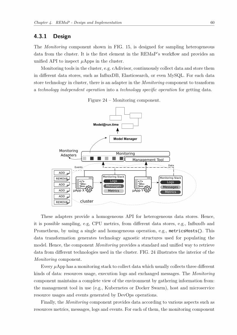
Chapter 4. REMaP - Design and Implementation 60

4.3.1 Design

The Monitoring component shown in FIG. 15, is designed for sampling heterogeneousdata from the cluster. It is the first element in the REMaP’s workflow and provides anunified API to inspect 𝜇Apps in the cluster.

Monitoring tools in the cluster, e.g. cAdivisor, continuously collect data and store themin different data stores, such as InfluxDB, Elasticsearch, or even MySQL. For each datastore technology in cluster, there is an adapter in the Monitoring component to transforma technology independent operation into a technology specific operation for getting data.

Figure 24 – Monitoring component.

Monitoring

μApp X μApp Y

Logs

Messages

Metrics

Monitoring Stack

Logs

Messages

Metrics

Monitoring Stack

cluster

MonitoringAdapters

Management Tool

Model@run.time

Model Manager

EventsData

ADD

REMOVE

ADD

ADD

ADD

REMOVE

These adapters provide a homogeneous API for heterogeneous data stores. Hence,it is possible sampling, e.g, CPU metrics, from different data stores, e.g., Influxdb andPrometheus, by using a single and homogeneous operation, e.g., metricsHosts(). Thisdata transformation generates technology agnostic structures used for populating themodel. Hence, the component Monitoring provides a standard and unified way to retrievedata from different technologies used in the cluster. FIG. 24 illustrates the interior of theMonitoring component.

Every 𝜇App has a monitoring stack to collect data which usually collects three differentkinds of data: resources usage, execution logs and exchanged messages. The Monitoringcomponent maintains a complete view of the environment by gathering information from:the management tool in use (e.g., Kubernetes or Docker Swarm), host and microserviceresource usages and events generated by DevOps operations.

Finally, the Monitoring component provides data according to various aspects such asresources metrics, messages, logs and events. For each of them, the monitoring component

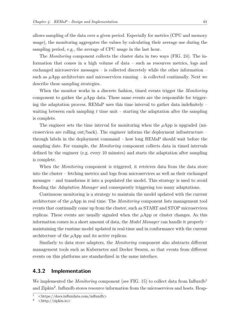
Chapter 4. REMaP - Design and Implementation 61

allows sampling of the data over a given period. Especially for metrics (CPU and memoryusage), the monitoring aggregates the values by calculating their average use during thesampling period, e.g., the average of CPU usage in the last hour.

The Monitoring component collects the cluster data in two ways (FIG. 24). The in-formation that comes in a high volume of data – such as resources metrics, logs andexchanged microservice messages – is collected discretely while the other information –such as 𝜇App architecture and microservices running – is collected continually. Next wedescribe these sampling strategies.

When the monitor works in a discrete fashion, timed events trigger the Monitoringcomponent to gather the 𝜇App data. These same events are the responsible for trigger-ing the adaptation process. REMaP uses this time interval to gather data indefinitely –waiting between each sampling t time unit – starting the adaptation after the samplingis complete.

The engineer sets the time interval for monitoring when the 𝜇App is upgraded (mi-croservices are rolling out/back). The engineer informs the deployment infrastructure –through labels in the deployment command – how long REMaP should wait before thesampling date. For example, the Monitoring component collects data in timed intervalsdefined by the engineer (e.g. every 10 minutes) and starts the adaptation after samplingis complete.

When the Monitoring component is triggered, it retrieves data from the data storeinto the cluster – fetching metrics and logs from microservices as well as their exchangedmessages – and transforms it into a populated the model. This strategy is used to avoidflooding the Adaptation Manager and consequently triggering too many adaptations.

Continuous monitoring is a strategy to maintain the model updated with the currentarchitecture of the 𝜇App in real time. The Monitoring component lists management toolevents that continually come up from the cluster, such as START and STOP microservicesreplicas. These events are usually signaled when the 𝜇App or cluster changes. As thisinformation comes in a short amount of data, the Model Manager can handle it properly –maintaining the runtime model updated in real-time and in conformance with the currentarchitecture of the 𝜇App and its active replicas.

Similarly to data store adapters, the Monitoring component also abstracts differentmanagement tools such as Kubernetes and Docker Swarm, so that events from differentevents on this platforms are standardized in the same interface.

4.3.2 Implementation

We implemented the Monitoring component (see FIG. 15) to collect data from Influxdb1

and Zipkin2. Influxdb stores resource information from the microservices and hosts. Heap-1 <https://docs.influxdata.com/influxdb>2 <http://zipkin.io>

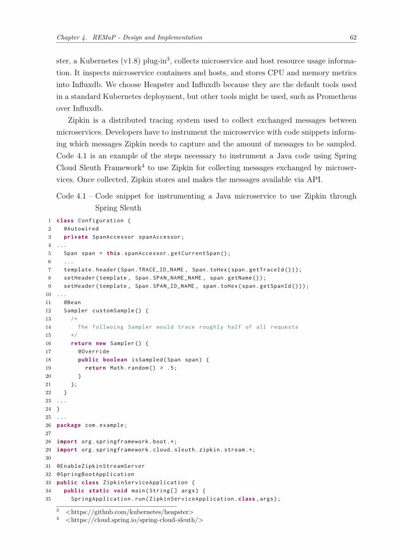
Chapter 4. REMaP - Design and Implementation 62

ster, a Kubernetes (v1.8) plug-in3, collects microservice and host resource usage informa-tion. It inspects microservice containers and hosts, and stores CPU and memory metricsinto Influxdb. We choose Heapster and Influxdb because they are the default tools usedin a standard Kubernetes deployment, but other tools might be used, such as Prometheusover Influxdb.

Zipkin is a distributed tracing system used to collect exchanged messages betweenmicroservices. Developers have to instrument the microservice with code snippets inform-ing which messages Zipkin needs to capture and the amount of messages to be sampled.Code 4.1 is an example of the steps necessary to instrument a Java code using SpringCloud Sleuth Framework4 to use Zipkin for collecting messages exchanged by microser-vices. Once collected, Zipkin stores and makes the messages available via API.

Code 4.1 – Code snippet for instrumenting a Java microservice to use Zipkin throughSpring Sleuth

1 class Configuration {

2 @Autowired

3 private SpanAccessor spanAccessor;

4 ...

5 Span span = this.spanAccessor.getCurrentSpan ();

6 ...

7 template.header(Span.TRACE_ID_NAME , Span.toHex(span.getTraceId ()));

8 setHeader(template , Span.SPAN_NAME_NAME , span.getName ());

9 setHeader(template , Span.SPAN_ID_NAME , span.toHex(span.getSpanId ()));

10 ...

11 @Bean

12 Sampler customSample () {

13 /*

14 The follwoing Sampler would trace roughly half of all requests

15 */

16 return new Sampler () {

17 @Override

18 public boolean isSampled(Span span) {

19 return Math.random () > .5;

20 }

21 };

22 }

23 ...

24 }

25 ...

26 package com.example;

2728 import org.springframework.boot .*;

29 import org.springframework.cloud.sleuth.zipkin.stream .*;

3031 @EnableZipkinStreamServer

32 @SpringBootApplication

33 public class ZipkinServiceApplication {

34 public static void main(String [] args) {

35 SpringApplication.run(ZipkinServiceApplication.class ,args);

3 <https://github.com/kubernetes/heapster>4 <https://cloud.spring.io/spring-cloud-sleuth/>

Chapter 4. REMaP - Design and Implementation 63

36 }

37 }

We also implemented a Kubernetes client to collect signals from the cluster and clusterconfiguration. Kubernetes has an API that provides cluster data (available hosts andrunning microservice instances); thus, whenever the cluster suffers some change, lika anew microservice replica, the client collects this data to update the model.

The monitoring component wraps the underlying monitoring technology and exposessome interfaces: MetricsInspectionInterface provides information about resources usage;MessagesInspectionInterface gives information about exchanged messages; and Cluster-InspectionInterface stores information about cluster data and organization – hosts andrunning microservice instances. These interfaces are combined into a InspectionInterface,Code 4.2, exposed by the monitoring.

Code 4.2 – Monitoring Interface1 interface ClusterInspectionInterface {

2 // list all hosts available in the cluster

3 List hosts();

4 // returns all services (including replicas) running in the cluster

5 List services ();

6 // returns all applications running in the cluster and the weight

7 // for calculate the affinities

8 Map <String , Float > application ();

9 // returns the management tool being used

10 String cluster ();

11 }

1213 interface MetricsInspectionInterface {

14 Map <String , Float > metricsMicroservice ()

15 // returns the metrics of all hosts in the last t seconds

16 Map <String , Float > metricsHosts(long timeInterval)

17 }

1819 interface MessagesInspectionInterface {

20 // returns all messages from the last t seconds

21 List messages(long timeInterval)

22 }

2324 interface InspectionInterface extends ClusterInspectionInterface ,

25 MessagesInspectionInterface , MetricsInspectionInterface {

26 }

Finally, the monitor also implements a listener to handle DevOps events. The listenerreceives events from Travis Travis5, a continuous integration tool that signals when a newdeployment event occurs (e.g. upgrading a 𝜇App). Hence, when engineers upgrade the𝜇App, the listener resets the timer in the adaptation engine – as described in Section 4.7.

All the data collected from different data sources is used to populate the model il-lustrated in FIG. 23. The ClusterInspectionInterface provides the data used for Model5 <https://travis-ci.org>

Chapter 4. REMaP - Design and Implementation 64

Manager instantiate the class that represent hosts, applications and microservices. In-ternally, the Monitoring component receives a continuous flow of events telling what ishappening in the cluster – microservices and hosts being instantiated or removed – andpassing them on to the model manager, to instantiate their related classes into the model.

The MetricsInspectionInterface provides the data used for the Model Manager to pop-ulate the microservice’s resource consumption and the host in the model. ComponentMonitoring gathers the metrics according to their types and targets – CPU usage ofmicroservices N – and Model Manager gets aggregations when they are triggered (Sec-tiondesign.monitoring.design). The calculated aggregation is the average of resource usagein a given interval (Section 4.3.1) – the average CPU usage in microservice N in last 10minutes.

Finally, MessagesInspectionInterface provides the data used to link the microservicesand to define the 𝜇App workflow. The Model Handler component gets the messagesexchanges by all microservices through the Monitoring component.

4.4 ANALYZERThe Analyzer component inspects the model in order to calculate the affinities betweenmicroservices. The messages exchanged by the microservices are collected and kept onthe model. The Analyzer examines the messages and – based on the number of messagesexchanged by two microservices as well as the size of the messages – calculates the degreeof affinity between two microservices.

4.4.1 Design

The Analyzer component, shown in FIG. 15, is designed to process the model at runtimeby looking for affinities between microservices. We define affinity by using the number ofmessages and the amount of data exchanged between them. We use a ratio (weight) inthe affinity calculation to steer the Analyzer execution. The data exchanged between themicroservices are not equally distributed among the exchanged messages. 𝜇App workflowswith few messages and a significant amount of data, and vice-versa, may exist. Hence, ahigh ratio value (> 0.5) leads the Analyzer to evaluate the number of messages over theamount of data. A small ratio value (< 0.5) does the opposite, and a ratio of 0.5 balancesthe two attributes equally.

The weight is set when the REMaP is installed to monitor the cluster. The clusterprovider (engineer) should set what weight REMaP will steer the adaptation.

In the general purpose of MAPE-K, the Analyzer component gets signals from mon-itoring named symptoms and, from these signals, detecting some aspect from the appli-cation or environment. In this work, we design an Affinity analyzer that detects affinities

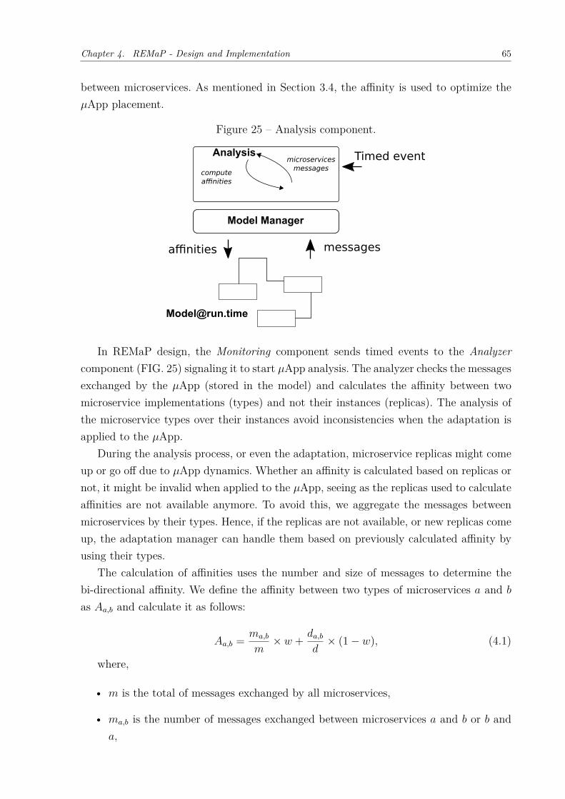
Chapter 4. REMaP - Design and Implementation 65

between microservices. As mentioned in Section 3.4, the affinity is used to optimize the𝜇App placement.

Figure 25 – Analysis component.

compute affinities

Analysismicroservices

messages

Model@run.time

Model Manager

affinities messages

Timed event

In REMaP design, the Monitoring component sends timed events to the Analyzercomponent (FIG. 25) signaling it to start 𝜇App analysis. The analyzer checks the messagesexchanged by the 𝜇App (stored in the model) and calculates the affinity between twomicroservice implementations (types) and not their instances (replicas). The analysis ofthe microservice types over their instances avoid inconsistencies when the adaptation isapplied to the 𝜇App.

During the analysis process, or even the adaptation, microservice replicas might comeup or go off due to 𝜇App dynamics. Whether an affinity is calculated based on replicas ornot, it might be invalid when applied to the 𝜇App, seeing as the replicas used to calculateaffinities are not available anymore. To avoid this, we aggregate the messages betweenmicroservices by their types. Hence, if the replicas are not available, or new replicas comeup, the adaptation manager can handle them based on previously calculated affinity byusing their types.

The calculation of affinities uses the number and size of messages to determine thebi-directional affinity. We define the affinity between two types of microservices 𝑎 and 𝑏

as 𝐴𝑎,𝑏 and calculate it as follows:

𝐴𝑎,𝑏 = 𝑚𝑎,𝑏

𝑚× 𝑤 + 𝑑𝑎,𝑏

𝑑× (1− 𝑤), (4.1)

where,

• 𝑚 is the total of messages exchanged by all microservices,

• 𝑚𝑎,𝑏 is the number of messages exchanged between microservices 𝑎 and 𝑏 or 𝑏 and𝑎,

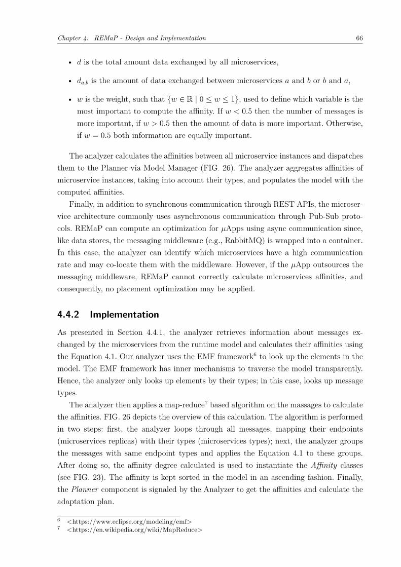
Chapter 4. REMaP - Design and Implementation 66

• 𝑑 is the total amount data exchanged by all microservices,

• 𝑑𝑎,𝑏 is the amount of data exchanged between microservices 𝑎 and 𝑏 or 𝑏 and 𝑎,

• 𝑤 is the weight, such that {𝑤 ∈ R | 0 ≤ 𝑤 ≤ 1}, used to define which variable is themost important to compute the affinity. If 𝑤 < 0.5 then the number of messages ismore important, if 𝑤 > 0.5 then the amount of data is more important. Otherwise,if 𝑤 = 0.5 both information are equally important.

The analyzer calculates the affinities between all microservice instances and dispatchesthem to the Planner via Model Manager (FIG. 26). The analyzer aggregates affinities ofmicroservice instances, taking into account their types, and populates the model with thecomputed affinities.

Finally, in addition to synchronous communication through REST APIs, the microser-vice architecture commonly uses asynchronous communication through Pub-Sub proto-cols. REMaP can compute an optimization for 𝜇Apps using async communication since,like data stores, the messaging middleware (e.g., RabbitMQ) is wrapped into a container.In this case, the analyzer can identify which microservices have a high communicationrate and may co-locate them with the middleware. However, if the 𝜇App outsources themessaging middleware, REMaP cannot correctly calculate microservices affinities, andconsequently, no placement optimization may be applied.

4.4.2 Implementation

As presented in Section 4.4.1, the analyzer retrieves information about messages ex-changed by the microservices from the runtime model and calculates their affinities usingthe Equation 4.1. Our analyzer uses the EMF framework6 to look up the elements in themodel. The EMF framework has inner mechanisms to traverse the model transparently.Hence, the analyzer only looks up elements by their types; in this case, looks up messagetypes.

The analyzer then applies a map-reduce7 based algorithm on the massages to calculatethe affinities. FIG. 26 depicts the overview of this calculation. The algorithm is performedin two steps: first, the analyzer loops through all messages, mapping their endpoints(microservices replicas) with their types (microservices types); next, the analyzer groupsthe messages with same endpoint types and applies the Equation 4.1 to these groups.After doing so, the affinity degree calculated is used to instantiate the Affinity classes(see FIG. 23). The affinity is kept sorted in the model in an ascending fashion. Finally,the Planner component is signaled by the Analyzer to get the affinities and calculate theadaptation plan.

6 <https://www.eclipse.org/modeling/emf>7 <https://en.wikipedia.org/wiki/MapReduce>

Chapter 4. REMaP - Design and Implementation 67

Figure 26 – Affinities calculation.

Msg: A1 -> B3, size: 3Msg: C2 -> D1, size: 2Msg: A1 -> B2, size: 2Msg: A2 -> B1, size: 5Msg: C1 -> D2, size: 1

Msg: A -> B, size: 3Msg: A -> B, size: 2Msg: A -> B, size: 5

Msg: C -> D, size: 2Msg: C -> D, size: 1

Msg: A -> B, size: 10, count: 3

Msg: C -> D, size: 3, count: 2

Affinity_AB: 0.68

Affinity_CD: 0.32

weight: 0.51

2

4

2

3

4.5 PLANNERThe Planner examines the model – which has affinities between microservices and themicroservice resources usage history – and resources available in the hosts. Using thisinformation, it decides how to apply the adaptation to the 𝜇App by computing the besthosts to place the microservices. The Planner adopts two strategies to compute the place-ment of microservices, a heuristic, which does not guarantee an optimal placement, andan algorithm that guarantees optimal placement. As a result, the Planner generates a listof movements in order to update the 𝜇App by changing the placement of a microservicefrom one host to another.

4.5.1 Design

The Planer component (FIG. 27) uses the model at runtime to get the affinities amongmicroservices and their resource usage history and uses this information to calculate anadaptation plan for 𝜇Apps. The adaptation plan is a list of movements that the Executorcomponent should carry out in the cluster, moving the microservices from a source hostto a target host.

We propose three Planners to compute the placement of microservices during anadaptation: Heuristic-based Affinity Planner (HBA), Optimal Affinity Planner (OA) anda variation of OA, named OAmodified Planner. All planners compute a new placementfor 𝜇Apps by reducing this problem to a multi-objective bin-packing problem. Since thisproblem is NP-Hard, we know that an optimal approach is unfeasible for large 𝜇Apps.Hence, we designed the heuristic version (HBA), to achieve quasi-optimal solutions forlarge 𝜇Apps, and the optimal version (OA), to achieve an optimal solutions for small𝜇Apps.

The size of a 𝜇App is related to the reference adopted such as the number of microser-vice types or the number of replicas running. For example: What is a big 𝜇App? Onehaving four types of microservices, each with a dozen replicas, or, one having ten typesof microservices, each having a single replica? In this work, we agreed to classify the size

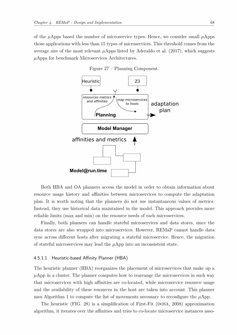
Chapter 4. REMaP - Design and Implementation 68

of the 𝜇Apps based the number of microservice types. Hence, we consider small 𝜇Appsthose applications with less than 15 types of microservices. This threshold comes from theaverage size of the most relevant 𝜇Apps listed by Aderaldo et al. (2017), which suggests𝜇Apps for benchmark Microservices Architectures.

Figure 27 – Planning Component.

Planning

map microservices to hosts

resources metricsand affinities

Model@run.time

Model Manager

affinities and metrics

adaptationplan

Heuristic Z3

Both HBA and OA planners access the model in order to obtain information aboutresource usage history and affinities between microservices to compute the adaptationplan. It is worth noting that the planners do not use instantaneous values of metrics.Instead, they use historical data maintained in the model. This approach provides morereliable limits (max and min) on the resource needs of each microservices.

Finally, both planners can handle stateful microservices and data stores, since thedata stores are also wrapped into microservices. However, REMaP cannot handle datasync across different hosts after migrating a stateful microservice. Hence, the migrationof stateful microservices may lead the 𝜇App into an inconsistent state.

4.5.1.1 Heuristic-based Affinity Planner (HBA)

The heuristic planner (HBA) reorganizes the placement of microservices that make up a𝜇App in a cluster. The planner computes how to rearrange the microservices in such waythat microservices with high affinities are co-located, while microservice resource usageand the availability of these resources in the host are taken into account. This planneruses Algorithm 1 to compute the list of movements necessary to reconfigure the 𝜇App.

The heuristic (FIG. 28) is a simplification of First-Fit (DOSA, 2008) approximationalgorithm, it iterates over the affinities and tries to co-locate microservice instances asso-

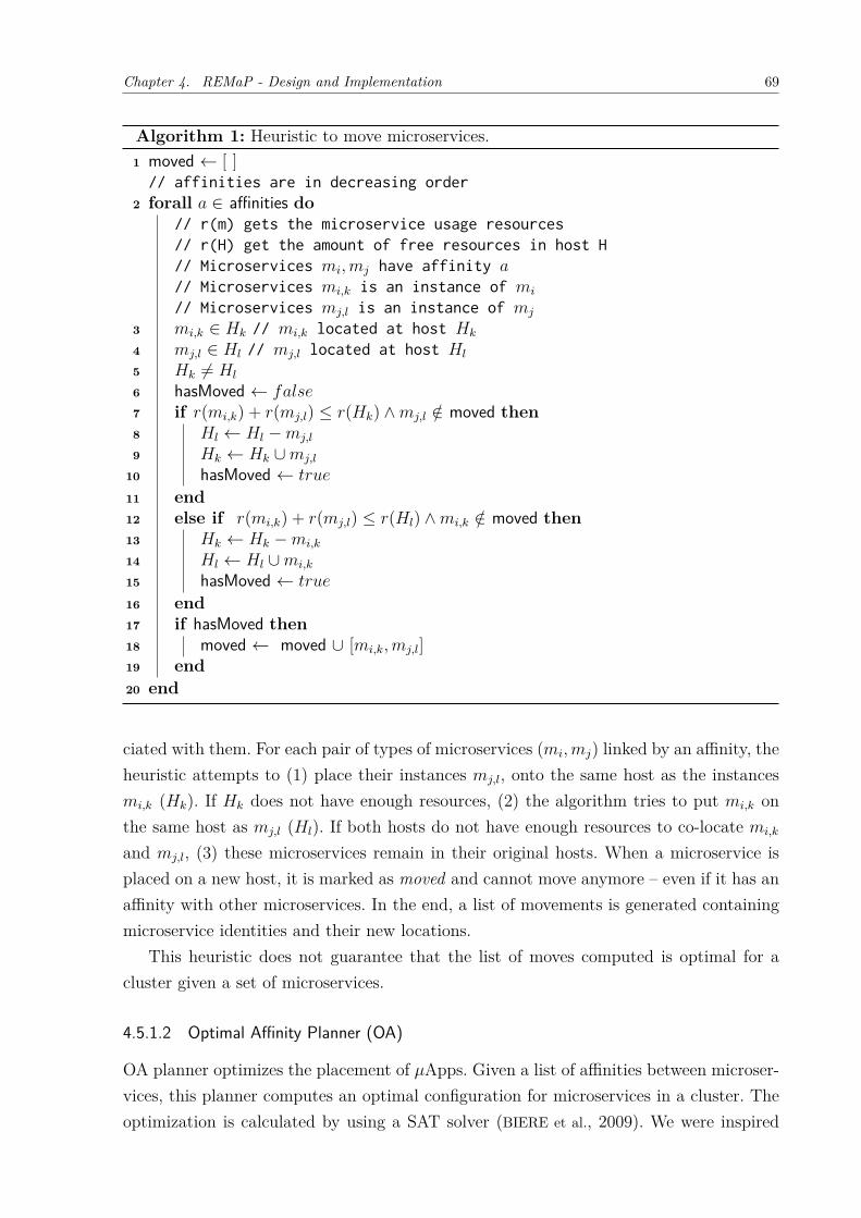
Chapter 4. REMaP - Design and Implementation 69

Algorithm 1: Heuristic to move microservices.1 moved ← [ ]// affinities are in decreasing order

2 forall 𝑎 ∈ affinities do// r(m) gets the microservice usage resources// r(H) get the amount of free resources in host H// Microservices 𝑚𝑖, 𝑚𝑗 have affinity 𝑎// Microservices 𝑚𝑖,𝑘 is an instance of 𝑚𝑖

// Microservices 𝑚𝑗,𝑙 is an instance of 𝑚𝑗

3 𝑚𝑖,𝑘 ∈ 𝐻𝑘 // 𝑚𝑖,𝑘 located at host 𝐻𝑘

4 𝑚𝑗,𝑙 ∈ 𝐻𝑙 // 𝑚𝑗,𝑙 located at host 𝐻𝑙

5 𝐻𝑘 ̸= 𝐻𝑙

6 hasMoved ← 𝑓𝑎𝑙𝑠𝑒7 if 𝑟(𝑚𝑖,𝑘) + 𝑟(𝑚𝑗,𝑙) ≤ 𝑟(𝐻𝑘) ∧𝑚𝑗,𝑙 /∈ moved then8 𝐻𝑙 ← 𝐻𝑙 −𝑚𝑗,𝑙

9 𝐻𝑘 ← 𝐻𝑘 ∪𝑚𝑗,𝑙

10 hasMoved ← 𝑡𝑟𝑢𝑒

11 end12 else if 𝑟(𝑚𝑖,𝑘) + 𝑟(𝑚𝑗,𝑙) ≤ 𝑟(𝐻𝑙) ∧𝑚𝑖,𝑘 /∈ moved then13 𝐻𝑘 ← 𝐻𝑘 −𝑚𝑖,𝑘

14 𝐻𝑙 ← 𝐻𝑙 ∪𝑚𝑖,𝑘

15 hasMoved ← 𝑡𝑟𝑢𝑒

16 end17 if hasMoved then18 moved ← moved ∪ [𝑚𝑖,𝑘, 𝑚𝑗,𝑙]19 end20 end

ciated with them. For each pair of types of microservices (𝑚𝑖, 𝑚𝑗) linked by an affinity, theheuristic attempts to (1) place their instances 𝑚𝑗,𝑙, onto the same host as the instances𝑚𝑖,𝑘 (𝐻𝑘). If 𝐻𝑘 does not have enough resources, (2) the algorithm tries to put 𝑚𝑖,𝑘 onthe same host as 𝑚𝑗,𝑙 (𝐻𝑙). If both hosts do not have enough resources to co-locate 𝑚𝑖,𝑘

and 𝑚𝑗,𝑙, (3) these microservices remain in their original hosts. When a microservice isplaced on a new host, it is marked as moved and cannot move anymore – even if it has anaffinity with other microservices. In the end, a list of movements is generated containingmicroservice identities and their new locations.

This heuristic does not guarantee that the list of moves computed is optimal for acluster given a set of microservices.

4.5.1.2 Optimal Affinity Planner (OA)

OA planner optimizes the placement of 𝜇Apps. Given a list of affinities between microser-vices, this planner computes an optimal configuration for microservices in a cluster. Theoptimization is calculated by using a SAT solver (BIERE et al., 2009). We were inspired

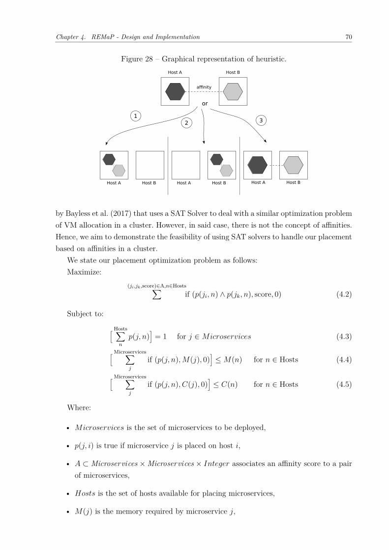
Chapter 4. REMaP - Design and Implementation 70

Figure 28 – Graphical representation of heuristic.

12 3

Host A Host AHost B Host B Host A Host B

affinity

Host A Host B

or

by Bayless et al. (2017) that uses a SAT Solver to deal with a similar optimization problemof VM allocation in a cluster. However, in said case, there is not the concept of affinities.Hence, we aim to demonstrate the feasibility of using SAT solvers to handle our placementbased on affinities in a cluster.

We state our placement optimization problem as follows:Maximize:

(𝑗𝑖,𝑗𝑘,score)∈A,𝑛∈Hosts∑︁if (𝑝(𝑗𝑖, 𝑛) ∧ 𝑝(𝑗𝑘, 𝑛), score, 0) (4.2)

Subject to:

[︁ Hosts∑︁𝑛

𝑝(𝑗, 𝑛)]︁

= 1 for 𝑗 ∈𝑀𝑖𝑐𝑟𝑜𝑠𝑒𝑟𝑣𝑖𝑐𝑒𝑠 (4.3)

[︁ Microservices∑︁𝑗

if (𝑝(𝑗, 𝑛), 𝑀(𝑗), 0)]︁≤𝑀(𝑛) for 𝑛 ∈ Hosts (4.4)

[︁ Microservices∑︁𝑗

if (𝑝(𝑗, 𝑛), 𝐶(𝑗), 0)]︁≤ 𝐶(𝑛) for 𝑛 ∈ Hosts (4.5)

Where:

• 𝑀𝑖𝑐𝑟𝑜𝑠𝑒𝑟𝑣𝑖𝑐𝑒𝑠 is the set of microservices to be deployed,

• 𝑝(𝑗, 𝑖) is true if microservice 𝑗 is placed on host 𝑖,

• 𝐴 ⊂ Microservices ×Microservices × 𝐼𝑛𝑡𝑒𝑔𝑒𝑟 associates an affinity score to a pairof microservices,

• 𝐻𝑜𝑠𝑡𝑠 is the set of hosts available for placing microservices,

• 𝑀(𝑗) is the memory required by microservice 𝑗,

Chapter 4. REMaP - Design and Implementation 71

• 𝑀(𝑛) is the memory available in host 𝑛,

• 𝐶(𝑗) is the number of cores required by microservice 𝑗, and

• 𝐶(𝑛) is the number of cores available in host 𝑛.

Equation 4.2 defines the objective function, maximizing the sum of affinity scores of allco-located microservices 𝑗𝑖, 𝑗𝑘. This equation returns 𝑠𝑐𝑜𝑟𝑒 if 𝑝(𝑗𝑖, 𝑛) ∧ 𝑝(𝑗𝑘, 𝑛) evaluatesto true and 0, otherwise.

Equation 4.3 is a constraint enforcing that each microservice instance should be placedon precisely one host, once a microservice is indivisible and cannot be placed in multiplehosts. For each microservice, the sum 𝑝(𝑗, 𝑛) over all hosts must be 1, meaning that foreach microservice 𝑗, 𝑝 must be true exactly once. Note that while a microservice can onlybe placed on one host, a host may have multiple microservices placed on it. Equation 4.4and Equation 4.5 ensure that each host has sufficient memory and cores to execute themicroservices.

This planner tries to minimize the number of hosts used to deploy a 𝜇App and max-imize the affinity scores on each host. In practice, The Equations 4.2 to 4.5 are usedto model the optimization algorithm to place microservices replicas with high affinitiestogether, considering host resources and microservice resource usage history.

Unlike the HBA planner, the OA planner guarantees that it finds an optimal placement– i.e. it minimizes wasted resources.

The designs of OA planner and OA-modify planner are the same and the difference isonly in their implementation details.

4.5.2 Implementation

The planner computes the movements to optimally re-arrange microservices. It creates alist of moves to transfer a microservice from one host to another and passes this list tothe model manager, which then forwards the list to the executor.

4.5.2.1 HBA Planner

This planner goes through each affinity generated by the analyzer and checks if it ispossible to move one of the microservices, as defined in Algorithm 1. If the movementis valid, it is stored in the Adaptation Script (Code 4.3). This script is a movement listinforming the source and destination of a microservice instance in a cluster.

Code 4.3 – Example of Adaptation Script1 class Moviment {

2 String microservice;

3 String source;

4 String destination;

Chapter 4. REMaP - Design and Implementation 72

5 ...

6 }

7 ...

89 List <Moviment > adaptationScript = new LinkedList <>();

10 ...

11 adaptationScript.add(new Moviment("usvc1", "hostA", "hostB")

12 adaptationScript.add(new Moviment("usvc2", "hostB", "hostC")

13 ...

14 adaptationScript.add(new Moviment("uscvN", "hostX", "hostZ")

15 ...

It is worth observing that only stateless microservices can be moved. As mentioned inSection 3.4.2, stateful microservice movement can raise issues on 𝜇Apps execution. Hence,we decided to add this constraint to the HBA planner.

To better illustrate this point, given microservices A.1 and B.1 running on hosts H.aand H.b, the planner checks if A.1 and B.1 fit in H.a. If possible, a movement is computedto move B.1 to H.a; otherwise, the planner checks if both microservices fit in H.b. In thiscase, a movement is computed to move A.1 to H.b. If neither microservices fit in H.anor H.b, then this affinity is discarded and the planner tries the next affinity. The HBAplanner only moves microservices to hosts where they already execute. In this example,microservices A.1 and B.1 can only be moved to hosts H.a or H.b.

After passing over all affinities, the planner forwards an Adaptation Script to theexecutor.

4.5.2.2 OA Planner

OA planner computes the placement of microservices using an SMT solver to calculatethe optimal arrangement of microservices in such a way as to minimize the number ofused hosts and maximize affinity scores for each host.

Our implementation uses Z38, a state-of-art SAT solver developed by Microsoft. Z3 isopen source, has a high performance and is widely used, which contributes to it havinggood documentation as a support by its community. The optimization is modelled as asatisfactory statement (BIERE et al., 2009) that can return optimal placement to a giveninput. However, SMT solvers usually use brute force to compute an optimization. Hence,as the placement of microservices is an NP-Hard problem, which makes it impossible forSMT solvers to handle large instances of the problem being solved in a reasonable time.

We choose Python wrapper for Z3 because they are better documented. Hence, OAPlanner is a Python script that receives the elements of the model necessary to computethe placement in JSON notation and uses the available methods in the Z3 wrapper toimplement equations presented in Section 4.5.1.2. The implementation of these equationsuses the specific syntax of Z3 – the complete code used by OA Planner – to calculate theoptimization depicted in Appendix A.8 <https://github.com/Z3Prover/z3>

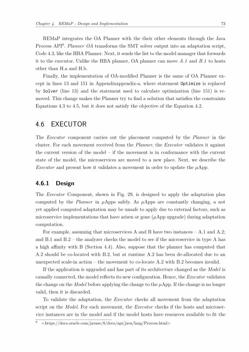
Chapter 4. REMaP - Design and Implementation 73

REMaP integrates the OA Planner with the their other elements through the JavaProcess API9. Planner OA transforms the SMT solver output into an adaptation script,Code 4.3, like the HBA Planner. Next, it sends the list to the model manager that forwardsit to the executor. Unlike the HBA planner, OA planner can move A.1 and B.1 to hostsother than H.a and H.b.

Finally, the implementation of OA-modified Planner is the same of OA Planner ex-cept in lines 13 and 151 in Appendixappendix-a, where statement Optimize is replacedby Solver (line 13) and the statement used to calculate optimization (line 151) is re-moved. This change makes the Planner try to find a solution that satisfies the constraintsEquations 4.3 to 4.5, but it does not satisfy the objective of the Equation 4.2.

4.6 EXECUTORThe Executor component carries out the placement computed by the Planner in thecluster. For each movement received from the Planner, the Executor validates it againstthe current version of the model – if the movement is in conformance with the currentstate of the model, the microservices are moved to a new place. Next, we describe theExecutor and present how it validates a movement in order to update the 𝜇App.

4.6.1 Design

The Executor Component, shown in Fig. 29, is designed to apply the adaptation plancomputed by the Planner in 𝜇Apps safely. As 𝜇Apps are constantly changing, a notyet applied computed adaptation may be unsafe to apply due to external factors, such asmicroservice implementations that have arisen or gone (𝜇App upgrade) during adaptationcomputation.

For example, assuming that microservices A and B have two instances – A.1 and A.2;and B.1 and B.2 – the analyzer checks the model to see if the microservice in type A hasa high affinity with B (Section 4.4). Also, suppose that the planner has computed thatA.2 should be co-located with B.2, but at runtime A.2 has been de-allocated due to anunexpected scale-in action – the movement to co-locate A.2 with B.2 becomes invalid.

If the application is upgraded and has part of its architecture changed as the Model iscausally connected, the model reflects its new configuration. Hence, the Executor validatesthe change on the Model before applying the change to the 𝜇App. If the change is no longervalid, then it is discarded.

To validate the adaptation, the Executor checks all movement from the adaptationscript on the Model. For each movement, the Executor checks if the hosts and microser-vice instances are in the model and if the model hosts have resources available to fit the9 <https://docs.oracle.com/javase/8/docs/api/java/lang/Process.html>

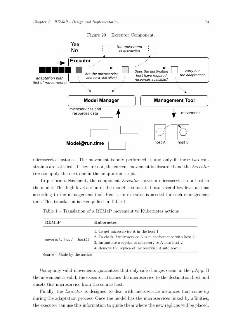
Chapter 4. REMaP - Design and Implementation 74

Figure 29 – Executor Component.

Executor

carry out the adaptation!Are the microservice

and host still alive?

Model@run.time

Model Manager

movementmicroservices and

resources data

adaptation plan(list of movements)

Management Tool

Does the destinationhost have required

resources available?

the movement is discardedNo

Yes

host A host B

microservice instance. The movement is only performed if, and only if, these two con-straints are satisfied. If they are not, the current movement is discarded and the Executortries to apply the next one in the adaptation script.

To perform a Movement, the component Executor moves a microservice to a host inthe model. This high level action in the model is translated into several low level actionsaccording to the management tool. Hence, an executor is needed for each managementtool. This translation is exemplified in Table 1.

Table 1 – Translation of a REMaP movement to Kubernetes actions

REMaP Kubernetes

move(msA, host1, host2)

1. To get microservice A in the host 12. To check if microservice A is in conformance with host 23. Instantiate a replica of microservice A into host 24. Remove the replica of microservice A into host 1

Source – Made by the author

Using only valid movements guarantees that only safe changes occur in the 𝜇App. Ifthe movement is valid, the executor attaches the microservice to the destination host andunsets this microservice from the source host.

Finally, the Executor is designed to deal with microservice instances that come upduring the adaptation process. Once the model has the microservices linked by affinities,the executor can use this information to guide them where the new replicas will be placed.

Chapter 4. REMaP - Design and Implementation 75

For example, given two microservices A and B with high affinity. Initially, there mightbe only replicas A.1 and B.1. However, during adaptation to co-locate A.1 and B.1, themicroservice B scales out and a B.2 replica is generated. The Executor will check themodel and find the affinity between A and B. First the Executor will attempt to co-locate B.2 with A.1. However, it rechecks if the model and the host, where A.1 is placed,do not fit another replica of B. So, the executor will try to co-locate B.2 with anothermicroservice instance so that both types have an affinity. If such microservice does notexist, the executor maintains replica B.2 at the host where it was instantiated.

4.6.2 Implementation

The component Executor wraps the management tool in the cluster. When the executorreceives the adaptation plan, it applies the moves one-by-one in the model. If a movecannot be applied, as discussed in Section 4.6.1, it is discarded – otherwise the moveis sent to the management tool wrapper, that applies it to the 𝜇App. Implementationcurrently includes wrappers for the most common management tools – Kubernetes andDocker Swarm. These tools are standard in cloud vendors that provide infrastructure forrunning 𝜇Apps.

In Kubernetes, it applies the changes by updating how the microservices are at-tached to the hosts in the deployment description maintained at runtime by changingthe nodeSelector labels of the microservices (Pods). Kubernetes goes through all ser-vices updating their placement attributes. Next, it executes the update by creating areplica of the updated microservice in a new host, starts the microservice and automati-cally removes the old one.

The process of how Kubernetes works internally to instantiate a microservice is outof scope of this thesis. A detailed explanation about this process can be found in (HAN-

NAFORD, 2017).Docker Swarm wrapper works similarly, we set labels and constraints to the hosts

and microservices to control the placement of microservices. However, unlike Kubernetes,Docker Swarm first removes the previous microservice and then creates a new replica inthe new location.

It is worth observing that in both wrappers, if the executor detects a failure afterapplying the changes, the adaptation process stops and the change is undone in both the𝜇App and model.

4.7 MODEL MANAGERThe Model Manager maintains the model at runtime, drawing it up and maintaining acausal connection between the model and the 𝜇App. The Model Manager coordinatesother REMaP components as well.

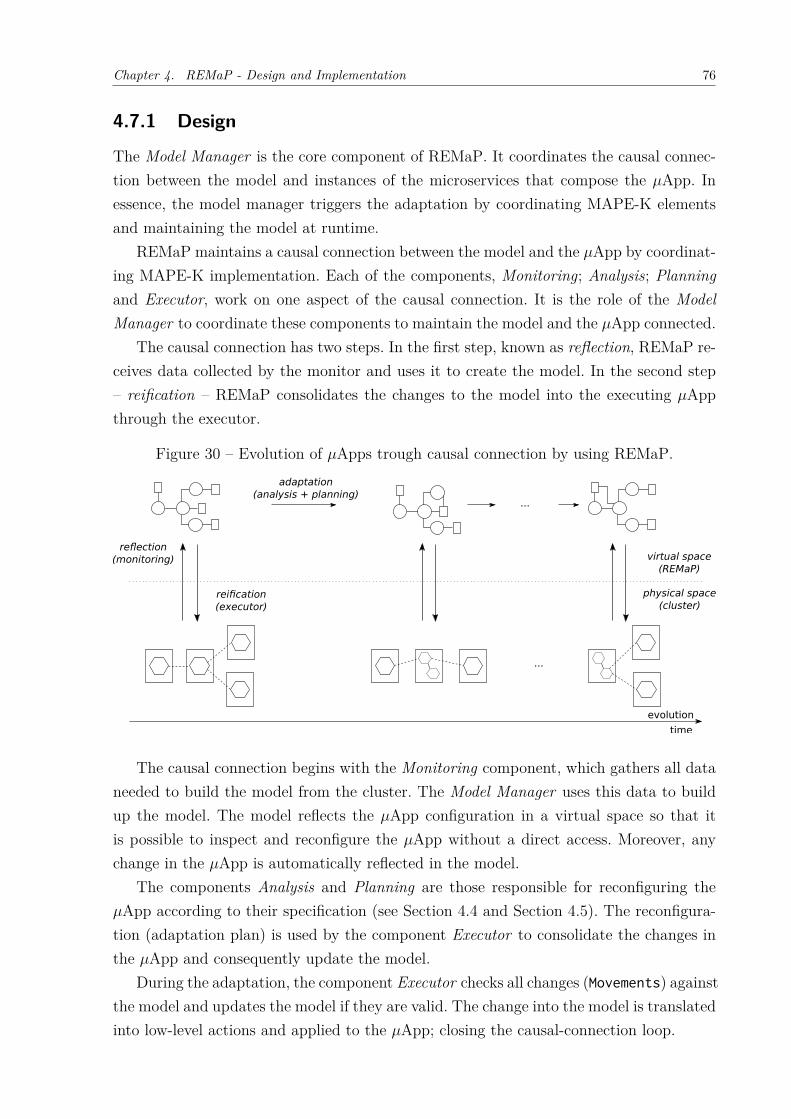
Chapter 4. REMaP - Design and Implementation 76

4.7.1 Design

The Model Manager is the core component of REMaP. It coordinates the causal connec-tion between the model and instances of the microservices that compose the 𝜇App. Inessence, the model manager triggers the adaptation by coordinating MAPE-K elementsand maintaining the model at runtime.

REMaP maintains a causal connection between the model and the 𝜇App by coordinat-ing MAPE-K implementation. Each of the components, Monitoring; Analysis; Planningand Executor, work on one aspect of the causal connection. It is the role of the ModelManager to coordinate these components to maintain the model and the 𝜇App connected.

The causal connection has two steps. In the first step, known as reflection, REMaP re-ceives data collected by the monitor and uses it to create the model. In the second step– reification – REMaP consolidates the changes to the model into the executing 𝜇Appthrough the executor.

Figure 30 – Evolution of 𝜇Apps trough causal connection by using REMaP.

...

time

reflection(monitoring)

reification(executor)

adaptation(analysis + planning)

evolution

...

virtual space(REMaP)

physical space(cluster)

The causal connection begins with the Monitoring component, which gathers all dataneeded to build the model from the cluster. The Model Manager uses this data to buildup the model. The model reflects the 𝜇App configuration in a virtual space so that itis possible to inspect and reconfigure the 𝜇App without a direct access. Moreover, anychange in the 𝜇App is automatically reflected in the model.

The components Analysis and Planning are those responsible for reconfiguring the𝜇App according to their specification (see Section 4.4 and Section 4.5). The reconfigura-tion (adaptation plan) is used by the component Executor to consolidate the changes inthe 𝜇App and consequently update the model.

During the adaptation, the component Executor checks all changes (Movements) againstthe model and updates the model if they are valid. The change into the model is translatedinto low-level actions and applied to the 𝜇App; closing the causal-connection loop.

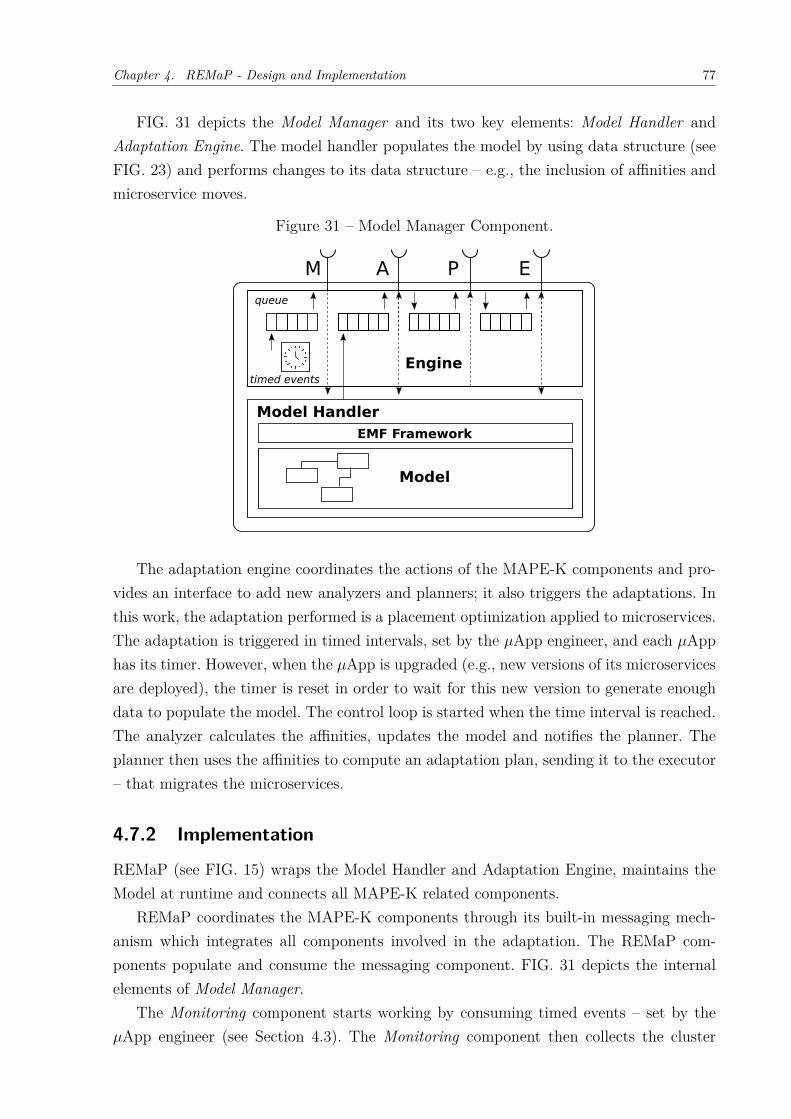
Chapter 4. REMaP - Design and Implementation 77

FIG. 31 depicts the Model Manager and its two key elements: Model Handler andAdaptation Engine. The model handler populates the model by using data structure (seeFIG. 23) and performs changes to its data structure – e.g., the inclusion of affinities andmicroservice moves.

Figure 31 – Model Manager Component.

timed eventsEngine

Model Handler

Model

M A P E

queue

EMF Framework

The adaptation engine coordinates the actions of the MAPE-K components and pro-vides an interface to add new analyzers and planners; it also triggers the adaptations. Inthis work, the adaptation performed is a placement optimization applied to microservices.The adaptation is triggered in timed intervals, set by the 𝜇App engineer, and each 𝜇Apphas its timer. However, when the 𝜇App is upgraded (e.g., new versions of its microservicesare deployed), the timer is reset in order to wait for this new version to generate enoughdata to populate the model. The control loop is started when the time interval is reached.The analyzer calculates the affinities, updates the model and notifies the planner. Theplanner then uses the affinities to compute an adaptation plan, sending it to the executor– that migrates the microservices.

4.7.2 Implementation

REMaP (see FIG. 15) wraps the Model Handler and Adaptation Engine, maintains theModel at runtime and connects all MAPE-K related components.

REMaP coordinates the MAPE-K components through its built-in messaging mech-anism which integrates all components involved in the adaptation. The REMaP com-ponents populate and consume the messaging component. FIG. 31 depicts the internalelements of Model Manager.

The Monitoring component starts working by consuming timed events – set by the𝜇App engineer (see Section 4.3). The Monitoring component then collects the cluster

Chapter 4. REMaP - Design and Implementation 78

data and sends it to the Model Manager, which consumes and uses the data to createmodel classes (see Section 4.2), while maintaining the model structure at runtime. Whenthe Model Handler builds the model, it notifies another queue, which is then consumedby the Analyzer. The Analyzer then consumes the notification and analyzes the model,signaling the Planner – in a similar way using a different queue – after it finishes. ThePlanner computes the adaptation plan, generating an adaptation script and pushing it tothe Executor ’s queue. Finally, the Executor consumes the script in the queue and carriesout the adaptation (Section 4.6).

Queue communication was designed foreseeing the evolution of REMaP’s implementa-tion, where each component might be a different process or microservice. This is a naturalevolution, since the model tends to be very large and making MAPE processing a machinemight be computationally expensive.

The Model Handler also uses the EMF framework to maintain the Model at runtime.EMF abstracts the construction/traversal of the model and provides a robust notificationmechanism to notify when the model changes – signalling these changes to other com-ponents. In our implementation, the Model Handler captures these signals to update thenumber of messages as well as the total data exchanged between the microservices.

When a message is attached to a microservice instance, EMF signals the Model Han-dler that the model was updated. The signal includes the message attributes. The EMFnotification uses actuators to update the microservice instance automatically by countingthe new message attached to it and the message size. Once the microservice instanceis updated, EMF signals to the Model Handler that the microservice was updated. Re-cursively, the EMF notification mechanism updates the application, counting the totalnumber of messages exchanged by the 𝜇App and the total amount of data exchanged.

REMaP uses the Adaptation Engine to handle a timed event to retrieve all messagesfrom the model, as described in Section 4.7.1. After an adaptation, the Model Managerneeds to wait for a while before building the model. This time is necessary because themodel is constructed using execution data collected from the 𝜇App (e.g., resource usage).In the current implementation, DevOps engineers are responsible for setting up this timedelay. This information is part of the event signalled during 𝜇App deployment, e.g., acustom message during a git push operation. The continuous delivery tool, Travis, handlesthe deployment of the microservices and notifies the Monitor – via a Web hook – whenthe building process is finished. Travis is also responsible for sending the custom messagesfrom the git push to the monitor telling how long to wait between the data gathering.

4.8 CONCLUDING REMARKSIn this chapter, we discussed the design and implementation of REMaP and how it is usedto improve the placement of 𝜇Apps at runtime. First, we presented the model used to keep

Chapter 4. REMaP - Design and Implementation 79

runtime information of 𝜇Apps and their primary elements. The model keeps the informa-tion collected by the component Monitoring. The Monitoring collects runtime informationof several aspects of 𝜇Apps at runtime. Next, we introduce the component Analyzer andits algorithm to calculate microservice affinities and how the messages exchanged by mi-croservices are used for this computation. The Analyzer calculates the affinity degreebetween all tuples of microservices in the 𝜇App based on the size and number of messagesexchanged by the microservices. Finally, we presented the component Planner and the dif-ferent strategies to calculate the placement adaptation of 𝜇Apps. Than, the componentExecutor carry out the adaptation on the 𝜇Apps deployed on Kubernetes and DockerSwarm. All components are integrated by the component Adaptation Manager whichcoordinates all REMaP’s components and maintains the causal connection between the𝜇App and the model.

80

5 EVALUATION

In this chapter, we evaluate the impact of REMaP on the 𝜇App adaptation consideringseveral different scenarios. Initially, we introduce the objectives of the evaluation followedby the set up of the experiments. Finally, we present the results along with their analysis.

5.1 OBJECTIVESAs presented in Chapter 4, REMaP is a mechanism used to carry out adaptations in𝜇Apps. As REMaP manages another software, we initially designed a set of experimentsto show the performance of individual components of REMaP itself. We then moved on tounderstand the impact of REMaP on 𝜇Apps, evaluating the impact on the performanceand resource usage of 𝜇Apps. These experiments can be detailed as follows:

1. Performance of REMaP components. As presented in Section 4.1, REMaP imple-ments the MAPE-K components and the duration of the adaptation depends on thetime spent in each of these components. Hence, we aim to identify those times tobetter understand the individual impact of the components.

2. Resources usage of 𝜇Apps. REMaP was developed to adapt 𝜇Apps by improvingtheir placement. This improvement usually reduces the number of hosts being usedby the 𝜇Apps. Hence, we aim to measure the gains made by REMaP on 𝜇Appresource usage.

3. Performance of 𝜇Apps. As shown in Section 4.5 REMaP co-locates high-affinity mi-croservices into a host to decrease the impact of the network latency in communica-tion. This strategy has a potential to reduce the time spent in the communicationbetween microservices, improving the overall performance of the 𝜇App. Hence, weaim to measure the improvements made by the adaptation on the 𝜇App’s perfor-mance.

Next, we describe the design of the experiments.

5.2 EXPERIMENTSWe used mock and empirical evaluations to assess the objectives mentioned before. Themock evaluation relies on using an entirely controlled scenario – the cluster and 𝜇Appsare modeled artificially as graphs that emulate the topologies of real 𝜇Apps with different

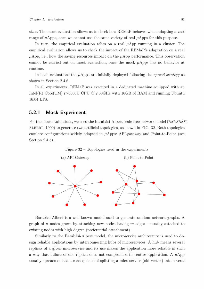
Chapter 5. Evaluation 81

sizes. The mock evaluation allows us to check how REMaP behaves when adapting a vastrange of 𝜇Apps, once we cannot use the same variety of real 𝜇Apps for this purpose.

In turn, the empirical evaluation relies on a real 𝜇App running in a cluster. Theempirical evaluation allows us to check the impact of the REMaP’s adaptation on a real𝜇App, i.e., how the saving resources impact on the 𝜇App performance. This observationcannot be carried out on mock evaluation, once the mock 𝜇Apps has no behavior atruntime.

In both evaluations the 𝜇Apps are initially deployed following the spread strategy asshown in Section 2.4.6.

In all experiments, REMaP was executed in a dedicated machine equipped with anIntel(R) Core(TM) i7-6500U CPU @ 2.50GHz with 16GB of RAM and running Ubuntu16.04 LTS.

5.2.1 Mock Experiment

For the mock evaluations, we used the Barabási-Albert scale-free network model (BARABÁSI;

ALBERT, 1999) to generate two artificial topologies, as shown in FIG. 32. Both topologiesemulate configurations widely adopted in 𝜇Apps: API-gateway and Point-to-Point (seeSection 2.4.5).

Figure 32 – Topologies used in the experiments

(a) API Gateway (b) Point-to-Point

Barabási-Albert is a well-known model used to generate random network graphs. Agraph of 𝑛 nodes grows by attaching new nodes having 𝑚 edges – usually attached toexisting nodes with high degree (preferential attachment).

Similarly to the Barabási-Albert model, the microservice architecture is used to de-sign reliable applications by interconnecting hubs of microservices. A hub means severalreplicas of a given microservice and its use makes the application more reliable in sucha way that failure of one replica does not compromise the entire application. A 𝜇Appusually spreads out as a consequence of splitting a microservice (old vertex) into several

Chapter 5. Evaluation 82

other microservices (new vertices). This feature motivates our use of the Barabási-Albertmodel to represent 𝜇Apps.

For consistency and reproductibility, we used the library NetworkX 1 to generatecomplex networks. We set the randomness seed to an arbitrary number (31) and ouralgorithm encapsulates the Barabási-Albert model function to guarantee that all graphsgenerated are connected like actual 𝜇Apps.

We set 𝑚 = 𝑛 − 1 and 𝑚 = 2 to generate the API-gateways (FIG. 32a) and Point-to-point (FIG. 32b) topologies. These values guarantee that the generated graphs havesimilar structures even with varying nodes (microservices) and edges (affinities).

For the generated graph, we labeled the microservices and hosts (vertex of the graph)with their resource usage; for microservices and their capacity, to the host. We used theresource usage of microservices with a uniform distribution: CPU over a 1 – 500 millicoresinterval and memory in the rage 10 – 500 MB. Hosts have 4000 millicores and 8GB ofmemory. Based on experiments performed on real 𝜇Apps and the analysis of deploymentfiles of different open-source 𝜇Apps available in the Internet, these values emulate anordinary configuration of business microservices in a 𝜇App.

The mock evaluation assesses the performance metrics, namely: time to compute theadaptation plan, time to compute each MAPE-K activity, time to carry out an adaptation,number of saved hosts, and resource usage to plan an adaptation. The time to compute anadaptation plan metric measures how long REMaP takes to calculate the adaptation. Themeasurement of this metric includes three phases: monitoring, analysis, and planning. Inthe end, the sum of the time to compute each of these phases gives us the time neededto calculate the adaptation plan. We use the impact of a component on the calculation ofadaptation plan metric to identify the impact, in percentage, of each REMaP componentin the total adaptation time.

The metric time to carry out the adaptation plan measures how long the 𝜇App man-agement tool (e.g., Kubernetes) takes to carry out the adaptation plan on the 𝜇App. Thenumber of saved hosts metric shows us how many hosts we can saved in a 𝜇App deploy-ment after carrying out the adaptation plan computed by REMaP. Finally, the resourceusage to plan an adaptation metric measures the CPU and memory utilization needed inorder to calculate an adaptation plan. Table 2 shows a summary of the metrics evaluatedin the mock experiment.

In the experiments, we used three different planners to compute the adaptation plan:HBA, OA (see Section 4.5), and a modified version of OA. This modified version calculatesplacement only considering the available resources in the host and microservices affinities,which means that it neither tries to maximize the affinities score in a host nor minimizethe number of hosts to be used. Moreover, the modified OA and OA planners use Z3’sbitvecs, a special 16 bits data type for integer numbers, to model data over integers with1 <https://networkx.github.io>

Chapter 5. Evaluation 83

Table 2 – Mock experiments metrics

Metric Evaluation Objective

Time to compute the adaptation plan To measure REMaP’s performanceTime to compute each MAPE-K activity To identify REMaP’s bottlenecksTime to carry out the adaptation plan To measure REMaP performance

Number of saved hosts To measure the amount or resourcessaved by using REMaP

32 bits. This strategy aims to decrease the search space during the calculation since theyuse a brute-force based strategy.

We conducted the mock experiments three times – changing the planner used to com-pute the adaptation plan (HBA Planner, OA Planner, and OA-modified Planner) eachtime. In these experiments we first measured the monitoring time of each topology – wegathered data stored in the monitoring stack of the mock 𝜇App to draw up the model.Next, we simulated several scenarios for 10 minutes – the time needed in order to collect105 messages using the proposed configuration, as shown in our empiric experiments. Inthe mock experiments we varied the number of messages exchanged by the microservices(101 to 105) and the number of microservices available (101 to 103) to see how these pa-rameters affected affinity computation. In the second step, we measured the time neededto compute the affinities, namely analysis time.

Finally, in the last step we measured the planning time by measuring the time neededto compute adaptation plans based on the affinities calculated in the previous step. More-over, we estimated the number of hosts we can save by applying the generated adaptationplans.

The number of movements computed by a planner is not proportional to the numberof microservices replicas and hosts in the model. Hence, we decided to create artificialmovements to evaluate the executor measuring execution time, i.e., the time to move themicroservice across different hosts. In this case, we measured the time to move 101 to 103

microservices using Kubernetes. We chose these numbers to emulate different real 𝜇Apps,since the size of real 𝜇Apps usually are not smaller than 10 microservices neither largerthan 1000. We choose Kubernetes because it is a widely used management tool. Table 3shows a summary of parameters and their values used in the mock experiments.

5.2.2 Empirical Experiment

For the empirical evaluation we used a reference 𝜇App named Sock-Shop2 (FIG. 33) –an open-source e-commerce 𝜇App of a site that sells socks –; widely used to evaluatemicroservices (ADERALDO et al., 2017). It has 15 microservices, five of which are state-2 <https://microservices-demo.github.io>

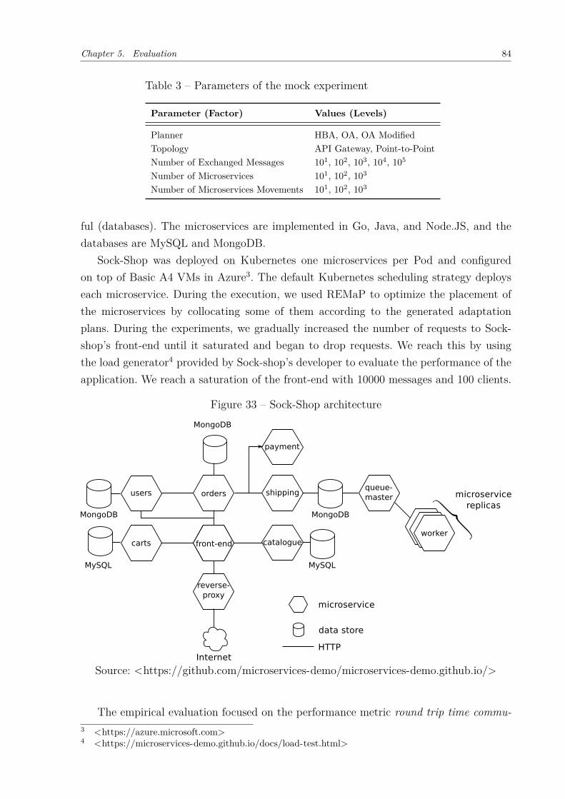
Chapter 5. Evaluation 84

Table 3 – Parameters of the mock experiment

Parameter (Factor) Values (Levels)

Planner HBA, OA, OA ModifiedTopology API Gateway, Point-to-PointNumber of Exchanged Messages 101, 102, 103, 104, 105

Number of Microservices 101, 102, 103

Number of Microservices Movements 101, 102, 103

ful (databases). The microservices are implemented in Go, Java, and Node.JS, and thedatabases are MySQL and MongoDB.

Sock-Shop was deployed on Kubernetes one microservices per Pod and configuredon top of Basic A4 VMs in Azure3. The default Kubernetes scheduling strategy deployseach microservice. During the execution, we used REMaP to optimize the placement ofthe microservices by collocating some of them according to the generated adaptationplans. During the experiments, we gradually increased the number of requests to Sock-shop’s front-end until it saturated and began to drop requests. We reach this by usingthe load generator4 provided by Sock-shop’s developer to evaluate the performance of theapplication. We reach a saturation of the front-end with 10000 messages and 100 clients.

Figure 33 – Sock-Shop architecture

Source: <https://github.com/microservices-demo/microservices-demo.github.io/>

The empirical evaluation focused on the performance metric round trip time commu-3 <https://azure.microsoft.com>4 <https://microservices-demo.github.io/docs/load-test.html>

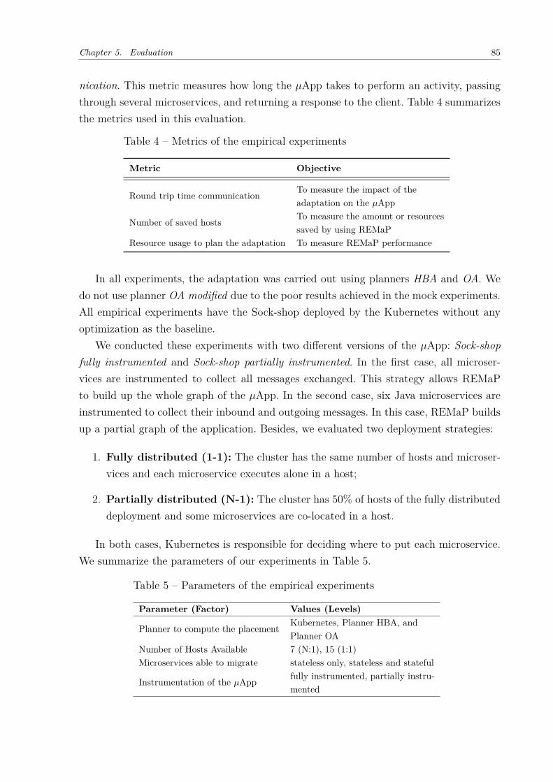
Chapter 5. Evaluation 85

nication. This metric measures how long the 𝜇App takes to perform an activity, passingthrough several microservices, and returning a response to the client. Table 4 summarizesthe metrics used in this evaluation.

Table 4 – Metrics of the empirical experiments

Metric Objective

Round trip time communication To measure the impact of theadaptation on the 𝜇App

Number of saved hosts To measure the amount or resourcessaved by using REMaP

Resource usage to plan the adaptation To measure REMaP performance

In all experiments, the adaptation was carried out using planners HBA and OA. Wedo not use planner OA modified due to the poor results achieved in the mock experiments.All empirical experiments have the Sock-shop deployed by the Kubernetes without anyoptimization as the baseline.

We conducted these experiments with two different versions of the 𝜇App: Sock-shopfully instrumented and Sock-shop partially instrumented. In the first case, all microser-vices are instrumented to collect all messages exchanged. This strategy allows REMaPto build up the whole graph of the 𝜇App. In the second case, six Java microservices areinstrumented to collect their inbound and outgoing messages. In this case, REMaP buildsup a partial graph of the application. Besides, we evaluated two deployment strategies:

1. Fully distributed (1-1): The cluster has the same number of hosts and microser-vices and each microservice executes alone in a host;

2. Partially distributed (N-1): The cluster has 50% of hosts of the fully distributeddeployment and some microservices are co-located in a host.

In both cases, Kubernetes is responsible for deciding where to put each microservice.We summarize the parameters of our experiments in Table 5.

Table 5 – Parameters of the empirical experiments

Parameter (Factor) Values (Levels)

Planner to compute the placement Kubernetes, Planner HBA, andPlanner OA

Number of Hosts Available 7 (N:1), 15 (1:1)Microservices able to migrate stateless only, stateless and stateful

Instrumentation of the 𝜇App fully instrumented, partially instru-mented

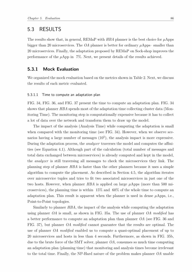
Chapter 5. Evaluation 86

5.3 RESULTSThe results show that, in general, REMaP with HBA planner is the best choice for 𝜇Appsbigger than 20 microservices. The OA planner is better for ordinary 𝜇Apps– smaller than20 microservices. Finally, the adaptation proposed by REMaP on Sock-shop improves theperformance of the 𝜇App in 7%. Next, we present details of the results achieved.

5.3.1 Mock Evaluation

We organized the mock evaluation based on the metrics shown in Table 2. Next, we discussthe results of each metric evaluated.

5.3.1.1 Time to compute an adaptation plan

FIG. 34, FIG. 36, and FIG. 37 present the time to compute an adaptation plan. FIG. 34shows that planner HBA spends most of the adaptation time collecting cluster data (Mon-itoring Time). The monitoring step is computationally expensive because it has to collecta lot of data over the network and transform them to draw up the model.

The impact of the analysis (Analysis Time) while computing the adaptation is smallwhen compared with the monitoring time (see FIG. 34). However, when we observe sce-narios having a large number of messages (105), the analysis impact is more expressive.During the adaptation process, the analyzer traverses the model and computes the affini-ties (see Equation 4.1). Although part of the calculation (total number of messages andtotal data exchanged between microservices) is already computed and kept in the model,the analyzer is still traversing all messages to check the microservices they link. Theplanning step of planner HBA is faster than the other planners because it uses a simplealgorithm to compute the placement. As described in Section 4.5, the algorithm iteratesover microservice tuples and tries to fit two associated microservices in just one of thetwo hosts. However, when planner HBA is applied on large 𝜇Apps (more than 500 mi-croservices), the planning time is within 15% and 60% of the whole time to compute anadaptation plan. This result is apparent when the planner is used in dense 𝜇Apps, i.e.,Point-to-Point topologies.

Similarly to planner HBA, the impact of the analysis while computing the adaptationusing planner OA is small, as shown in FIG. 35a. The use of planner OA modified hasa better performance to compute an adaptation plan than planner OA (see FIG. 36 andFIG. 37), but planner OA modified cannot guarantee that the results are optimal. Theuse of planner OA modified enabled us to compute a quasi-optimal placement of up to20 microservices and hosts in less than 4 seconds. Furthermore, as shown in FIG. 35b,due to the brute force of the SMT solver, planner OA, consumes so much time computingan adaptation plan (planning time) that monitoring and analysis times become irrelevantto the total time. Finally, the NP-Hard nature of the problem makes planner OA unable

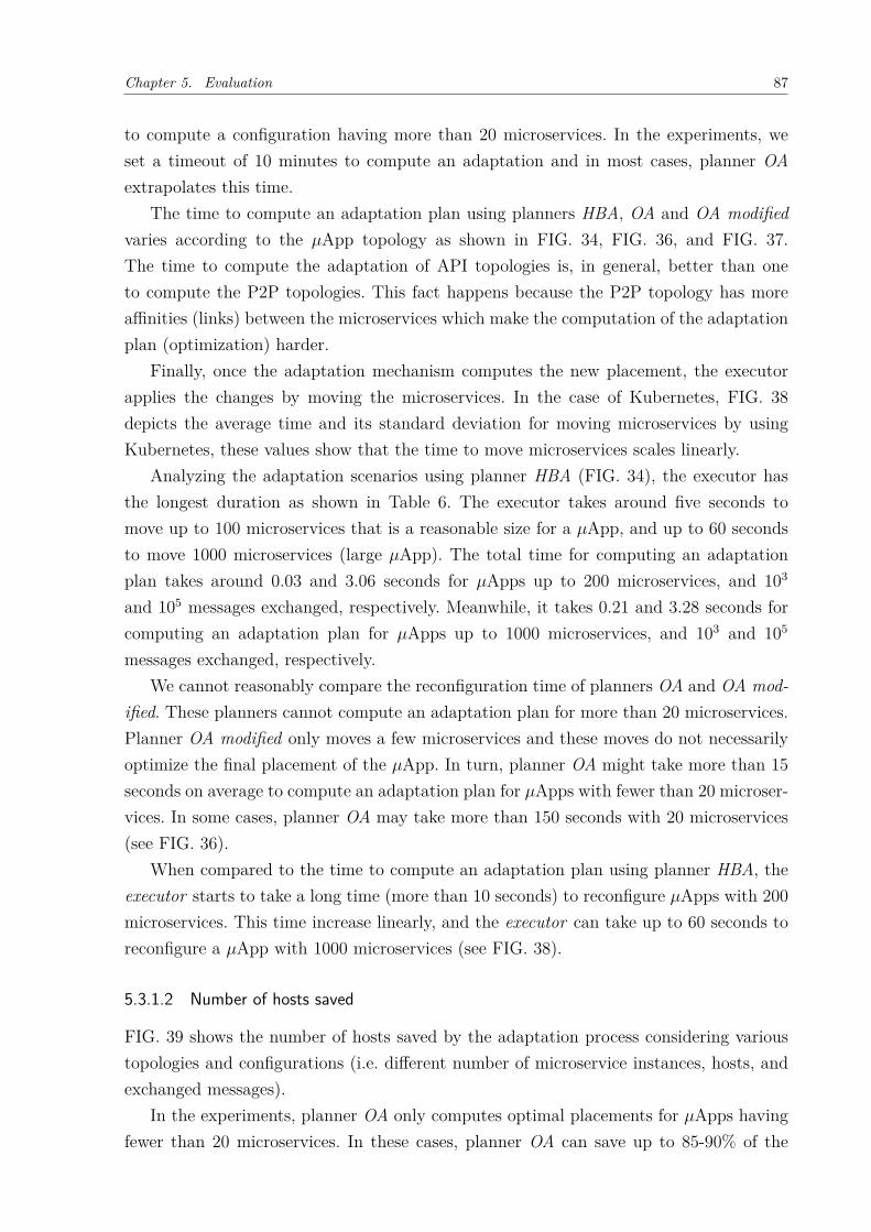
Chapter 5. Evaluation 87

to compute a configuration having more than 20 microservices. In the experiments, weset a timeout of 10 minutes to compute an adaptation and in most cases, planner OAextrapolates this time.

The time to compute an adaptation plan using planners HBA, OA and OA modifiedvaries according to the 𝜇App topology as shown in FIG. 34, FIG. 36, and FIG. 37.The time to compute the adaptation of API topologies is, in general, better than oneto compute the P2P topologies. This fact happens because the P2P topology has moreaffinities (links) between the microservices which make the computation of the adaptationplan (optimization) harder.

Finally, once the adaptation mechanism computes the new placement, the executorapplies the changes by moving the microservices. In the case of Kubernetes, FIG. 38depicts the average time and its standard deviation for moving microservices by usingKubernetes, these values show that the time to move microservices scales linearly.

Analyzing the adaptation scenarios using planner HBA (FIG. 34), the executor hasthe longest duration as shown in Table 6. The executor takes around five seconds tomove up to 100 microservices that is a reasonable size for a 𝜇App, and up to 60 secondsto move 1000 microservices (large 𝜇App). The total time for computing an adaptationplan takes around 0.03 and 3.06 seconds for 𝜇Apps up to 200 microservices, and 103

and 105 messages exchanged, respectively. Meanwhile, it takes 0.21 and 3.28 seconds forcomputing an adaptation plan for 𝜇Apps up to 1000 microservices, and 103 and 105

messages exchanged, respectively.We cannot reasonably compare the reconfiguration time of planners OA and OA mod-

ified. These planners cannot compute an adaptation plan for more than 20 microservices.Planner OA modified only moves a few microservices and these moves do not necessarilyoptimize the final placement of the 𝜇App. In turn, planner OA might take more than 15seconds on average to compute an adaptation plan for 𝜇Apps with fewer than 20 microser-vices. In some cases, planner OA may take more than 150 seconds with 20 microservices(see FIG. 36).

When compared to the time to compute an adaptation plan using planner HBA, theexecutor starts to take a long time (more than 10 seconds) to reconfigure 𝜇Apps with 200microservices. This time increase linearly, and the executor can take up to 60 seconds toreconfigure a 𝜇App with 1000 microservices (see FIG. 38).

5.3.1.2 Number of hosts saved

FIG. 39 shows the number of hosts saved by the adaptation process considering varioustopologies and configurations (i.e. different number of microservice instances, hosts, andexchanged messages).

In the experiments, planner OA only computes optimal placements for 𝜇Apps havingfewer than 20 microservices. In these cases, planner OA can save up to 85-90% of the

Chapter 5. Evaluation 88

Figure 34 – Time to compute an adaptation plan - HBA Planner

(a) 101 messages

(b) 102 messages

(c) 103 messages

(d) 104 messages

(e) 105 messages

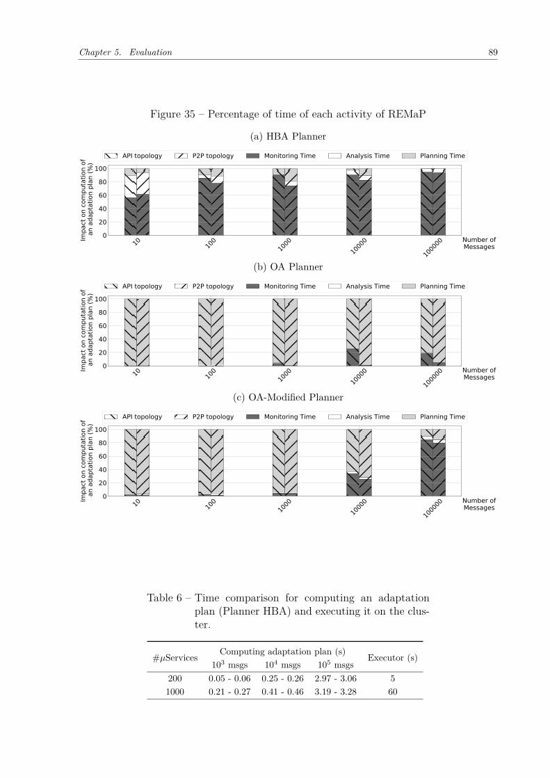
Chapter 5. Evaluation 89

Figure 35 – Percentage of time of each activity of REMaP

(a) HBA Planner

10 100

1000

1000

0

1000

00 Number ofMessages

020406080

100

Impa

ct o

n co

mpu

tatio

n of

an

adap

tatio

n pl

an (%

)

API topology P2P topology Monitoring Time Analysis Time Planning Time

(b) OA Planner

10 100

1000

1000

0

1000

00 Number ofMessages

020406080

100

Impa

ct o

n co

mpu

tatio

n of

an

adap

tatio

n pl

an (%

)

API topology P2P topology Monitoring Time Analysis Time Planning Time

(c) OA-Modified Planner

10 100

1000

1000

0

1000

00 Number ofMessages

020406080

100

Impa

ct o

n co

mpu

tatio

n of

an

adap

tatio

n pl

an (%

)

API topology P2P topology Monitoring Time Analysis Time Planning Time

Table 6 – Time comparison for computing an adaptationplan (Planner HBA) and executing it on the clus-ter.

#𝜇Services Computing adaptation plan (s) Executor (s)103 msgs 104 msgs 105 msgs

200 0.05 - 0.06 0.25 - 0.26 2.97 - 3.06 51000 0.21 - 0.27 0.41 - 0.46 3.19 - 3.28 60

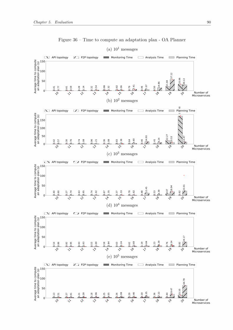
Chapter 5. Evaluation 90

Figure 36 – Time to compute an adaptation plan - OA Planner

(a) 101 messages

(b) 102 messages

(c) 103 messages

(d) 104 messages

(e) 105 messages

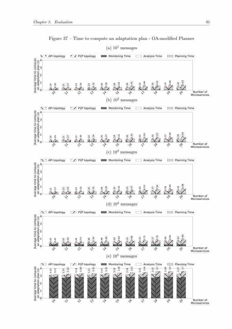
Chapter 5. Evaluation 91

Figure 37 – Time to compute an adaptation plan - OA-modified Planner

(a) 101 messages

(b) 102 messages

(c) 103 messages

(d) 104 messages

(e) 105 messages

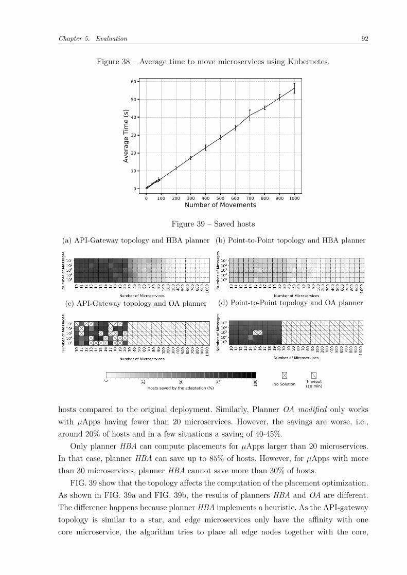
Chapter 5. Evaluation 92

Figure 38 – Average time to move microservices using Kubernetes.

0 100 200 300 400 500 600 700 800 900 1000Number of Movements

0

10

20

30

40

50

60

Aver

age

Tim

e (s

)

Figure 39 – Saved hosts

(a) API-Gateway topology and HBA planner (b) Point-to-Point topology and HBA planner

(c) API-Gateway topology and OA planner (d) Point-to-Point topology and OA planner

hosts compared to the original deployment. Similarly, Planner OA modified only workswith 𝜇Apps having fewer than 20 microservices. However, the savings are worse, i.e.,around 20% of hosts and in a few situations a saving of 40-45%.

Only planner HBA can compute placements for 𝜇Apps larger than 20 microservices.In that case, planner HBA can save up to 85% of hosts. However, for 𝜇Apps with morethan 30 microservices, planner HBA cannot save more than 30% of hosts.

FIG. 39 show that the topology affects the computation of the placement optimization.As shown in FIG. 39a and FIG. 39b, the results of planners HBA and OA are different.The difference happens because planner HBA implements a heuristic. As the API-gatewaytopology is similar to a star, and edge microservices only have the affinity with onecore microservice, the algorithm tries to place all edge nodes together with the core,

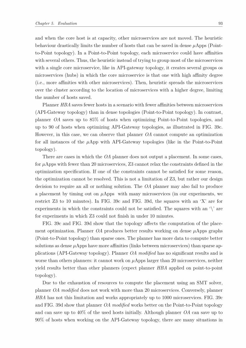
Chapter 5. Evaluation 93

and when the core host is at capacity, other microservices are not moved. The heuristicbehaviour drastically limits the number of hosts that can be saved in dense 𝜇Apps (Point-to-Point topology). In a Point-to-Point topology, each microservice could have affinitieswith several others. Thus, the heuristic instead of trying to group most of the microserviceswith a single core microservice, like in API-gateway topology, it creates several groups osmicroservices (hubs) in which the core microservice is that one with high affinity degree(i.e., more affinities with other microservices). Then, heuristic spreads the microservicesover the cluster according to the location of microservices with a higher degree, limitingthe number of hosts saved.

Planner HBA saves fewer hosts in a scenario with fewer affinities between microservices(API-Gateway topology) than in dense topologies (Point-to-Point topology). In contrast,planner OA saves up to 85% of hosts when optimizing Point-to-Point topologies, andup to 90 of hosts when optimizing API-Gateway topologies, as illustrated in FIG. 39c.However, in this case, we can observe that planner OA cannot compute an optimizationfor all instances of the 𝜇App with API-Gateway topologies (like in the Point-to-Pointtopology).

There are cases in which the OA planner does not output a placement. In some cases,for 𝜇Apps with fewer than 20 microservices, Z3 cannot relax the constraints defined in theoptimization specification. If one of the constraints cannot be satisfied for some reason,the optimization cannot be resolved. This is not a limitation of Z3, but rather our designdecision to require an all or nothing solution. The OA planner may also fail to producea placement by timing out on 𝜇Apps with many microservices (in our experiments, werestrict Z3 to 10 minutes). In FIG. 39c and FIG. 39d, the squares with an ‘X’ are forexperiments in which the constraints could not be satisfied. The squares with an ‘\’ arefor experiments in which Z3 could not finish in under 10 minutes.

FIG. 39c and FIG. 39d show that the topology affects the computation of the place-ment optimization. Planner OA produces better results working on dense 𝜇Apps graphs(Point-to-Point topology) than sparse ones. The planner has more data to compute bettersolutions as dense 𝜇Apps have more affinities (links between microservices) than sparse ap-plications (API-Gateway topology). Planner OA modified has no significant results and isworse than others planners: it cannot work on 𝜇Apps larger than 20 microservices, neitheryield results better than other planners (expect planner HBA applied on point-to-pointtopology).

Due to the exhaustion of resources to compute the placement using an SMT solver,planner OA modified does not work with more than 20 microservices. Conversely, plannerHBA has not this limitation and works appropriately up to 1000 microservices. FIG. 39cand FIG. 39d show that planner OA modified works better on the Point-to-Point topologyand can save up to 40% of the used hosts initially. Although planner OA can save up to90% of hosts when working on the API-Gateway topology, there are many situations in

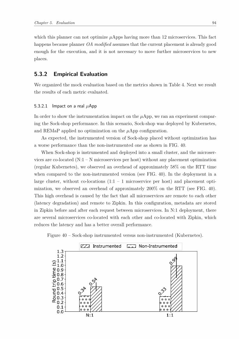
Chapter 5. Evaluation 94

which this planner can not optimize 𝜇Apps having more than 12 microservices. This facthappens because planner OA modified assumes that the current placement is already goodenough for the execution, and it is not necessary to move further microservices to newplaces.

5.3.2 Empirical Evaluation

We organized the mock evaluation based on the metrics shown in Table 4. Next we resultthe results of each metric evaluated.

5.3.2.1 Impact on a real 𝜇App

In order to show the instrumentation impact on the 𝜇App, we ran an experiment compar-ing the Sock-shop performance. In this scenario, Sock-shop was deployed by Kubernetes,and REMaP applied no optimization on the 𝜇App configuration.

As expected, the instrumented version of Sock-shop placed without optimization hasa worse performance than the non-instrumented one as shown in FIG. 40.

When Sock-shop is instrumented and deployed into a small cluster, and the microser-vices are co-located (N:1 – N microservices per host) without any placement optimization(regular Kubernetes), we observed an overhead of approximately 58% on the RTT timewhen compared to the non-instrumented version (see FIG. 40). In the deployment in alarge cluster, without co-locations (1:1 – 1 microservice per host) and placement opti-mization, we observed an overhead of approximately 200% on the RTT (see FIG. 40).This high overhead is caused by the fact that all microservices are remote to each other(latency degradation) and remote to Zipkin. In this configuration, metadata are storedin Zipkin before and after each request between microservices. In N:1 deployment, thereare several microservices co-located with each other and co-located with Zipkin, whichreduces the latency and has a better overall performance.

Figure 40 – Sock-shop instrumented versus non-instrumented (Kubernetes).

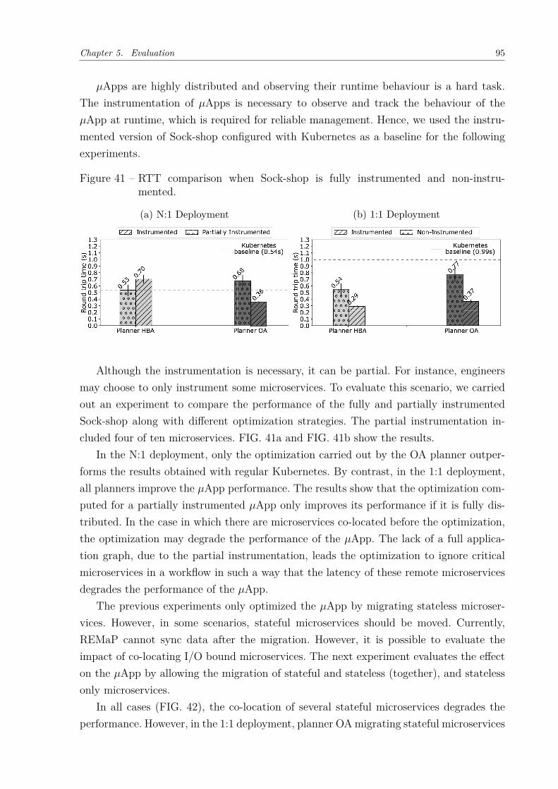
Chapter 5. Evaluation 95

𝜇Apps are highly distributed and observing their runtime behaviour is a hard task.The instrumentation of 𝜇Apps is necessary to observe and track the behaviour of the𝜇App at runtime, which is required for reliable management. Hence, we used the instru-mented version of Sock-shop configured with Kubernetes as a baseline for the followingexperiments.

Figure 41 – RTT comparison when Sock-shop is fully instrumented and non-instru-mented.

(a) N:1 Deployment (b) 1:1 Deployment

Although the instrumentation is necessary, it can be partial. For instance, engineersmay choose to only instrument some microservices. To evaluate this scenario, we carriedout an experiment to compare the performance of the fully and partially instrumentedSock-shop along with different optimization strategies. The partial instrumentation in-cluded four of ten microservices. FIG. 41a and FIG. 41b show the results.

In the N:1 deployment, only the optimization carried out by the OA planner outper-forms the results obtained with regular Kubernetes. By contrast, in the 1:1 deployment,all planners improve the 𝜇App performance. The results show that the optimization com-puted for a partially instrumented 𝜇App only improves its performance if it is fully dis-tributed. In the case in which there are microservices co-located before the optimization,the optimization may degrade the performance of the 𝜇App. The lack of a full applica-tion graph, due to the partial instrumentation, leads the optimization to ignore criticalmicroservices in a workflow in such a way that the latency of these remote microservicesdegrades the performance of the 𝜇App.

The previous experiments only optimized the 𝜇App by migrating stateless microser-vices. However, in some scenarios, stateful microservices should be moved. Currently,REMaP cannot sync data after the migration. However, it is possible to evaluate theimpact of co-locating I/O bound microservices. The next experiment evaluates the effecton the 𝜇App by allowing the migration of stateful and stateless (together), and statelessonly microservices.

In all cases (FIG. 42), the co-location of several stateful microservices degrades theperformance. However, in the 1:1 deployment, planner OA migrating stateful microservices

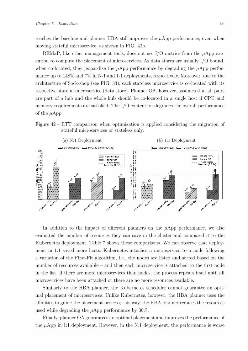
Chapter 5. Evaluation 96

reaches the baseline and planner HBA still improves the 𝜇App performance, even whenmoving stateful microservice, as shown in FIG. 42b.

REMaP, like other management tools, does not use I/O metrics from the 𝜇App exe-cution to compute the placement of microservices. As data stores are usually I/O bound,when co-located, they jeopardize the 𝜇App performance by degrading the 𝜇App perfor-mance up to 148% and 7% in N-1 and 1-1 deployments, respectively. Moreover, due to thearchitecture of Sock-shop (see FIG. 33), each stateless microservice is co-located with itsrespective stateful microservice (data store). Planner OA, however, assumes that all pairsare part of a hub and the whole hub should be co-located in a single host if CPU andmemory requirements are satisfied. The I/O contention degrades the overall performanceof the 𝜇App.

Figure 42 – RTT comparison when optimization is applied considering the migration ofstateful microservices or stateless only.

(a) N:1 Deployment (b) 1:1 Deployment

In addition to the impact of different planners on the 𝜇App performance, we alsoevaluated the number of resources they can save in the cluster and compared it to theKubernetes deployment. Table 7 shows these comparisons. We can observe that deploy-ment in 1:1 saved more hosts. Kubernetes attaches a microservice to a node followinga variation of the First-Fit algorithm, i.e., the nodes are listed and sorted based on thenumber of resources available – and then each microservice is attached to the first nodein the list. If there are more microservices than nodes, the process repeats itself until allmicroservices have been attached or there are no more resources available.

Similarly to the HBA planner, the Kubernetes scheduler cannot guarantee an opti-mal placement of microservices. Unlike Kubernetes, however, the HBA planner uses theaffinities to guide the placement process; this way, the HBA planner reduces the resourcesused while degrading the 𝜇App performance by 30%.

Finally, planner OA guarantees an optimal placement and improves the performance ofthe 𝜇App in 1:1 deployment. However, in the N:1 deployment, the performance is worse

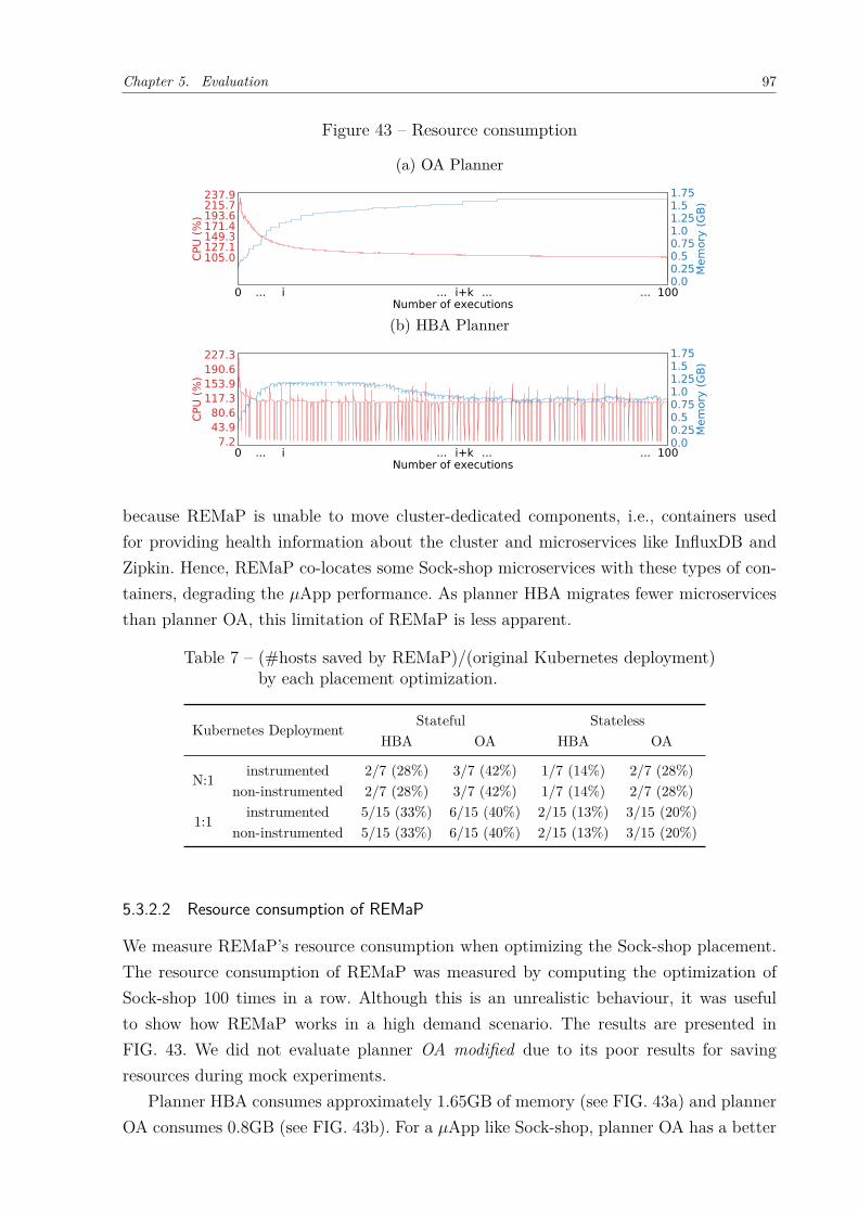
Chapter 5. Evaluation 97

Figure 43 – Resource consumption

(a) OA Planner

0 ... i ... i+k ... ... 100Number of executions

105.0127.1149.3171.4193.6215.7237.9

CPU

(%)

0.00.250.50.751.01.251.51.75

Mem

ory

(GB)

(b) HBA Planner

0 ... i ... i+k ... ... 100Number of executions

7.243.980.6

117.3153.9190.6227.3

CPU

(%)

0.00.250.50.751.01.251.51.75

Mem

ory

(GB)

because REMaP is unable to move cluster-dedicated components, i.e., containers usedfor providing health information about the cluster and microservices like InfluxDB andZipkin. Hence, REMaP co-locates some Sock-shop microservices with these types of con-tainers, degrading the 𝜇App performance. As planner HBA migrates fewer microservicesthan planner OA, this limitation of REMaP is less apparent.

Table 7 – (#hosts saved by REMaP)/(original Kubernetes deployment)by each placement optimization.

Kubernetes Deployment Stateful StatelessHBA OA HBA OA

N:1 instrumented 2/7 (28%) 3/7 (42%) 1/7 (14%) 2/7 (28%)non-instrumented 2/7 (28%) 3/7 (42%) 1/7 (14%) 2/7 (28%)

1:1 instrumented 5/15 (33%) 6/15 (40%) 2/15 (13%) 3/15 (20%)non-instrumented 5/15 (33%) 6/15 (40%) 2/15 (13%) 3/15 (20%)

5.3.2.2 Resource consumption of REMaP

We measure REMaP’s resource consumption when optimizing the Sock-shop placement.The resource consumption of REMaP was measured by computing the optimization ofSock-shop 100 times in a row. Although this is an unrealistic behaviour, it was usefulto show how REMaP works in a high demand scenario. The results are presented inFIG. 43. We did not evaluate planner OA modified due to its poor results for savingresources during mock experiments.

Planner HBA consumes approximately 1.65GB of memory (see FIG. 43a) and plannerOA consumes 0.8GB (see FIG. 43b). For a 𝜇App like Sock-shop, planner OA has a better

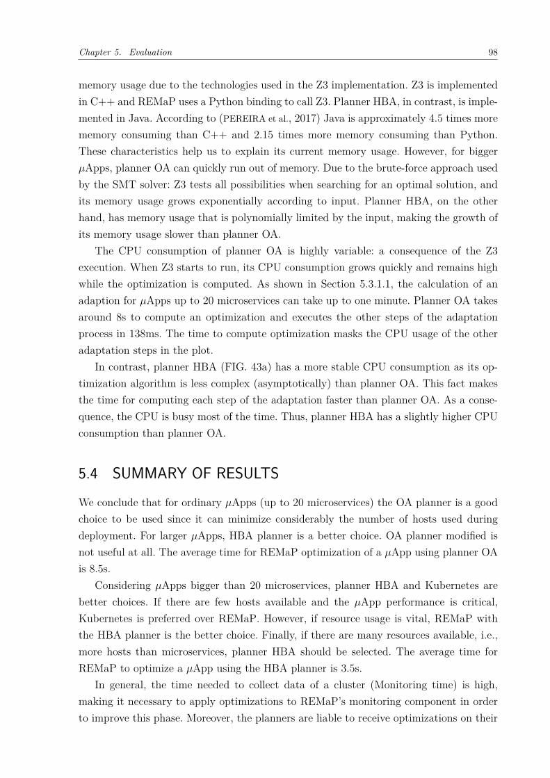
Chapter 5. Evaluation 98

memory usage due to the technologies used in the Z3 implementation. Z3 is implementedin C++ and REMaP uses a Python binding to call Z3. Planner HBA, in contrast, is imple-mented in Java. According to (PEREIRA et al., 2017) Java is approximately 4.5 times morememory consuming than C++ and 2.15 times more memory consuming than Python.These characteristics help us to explain its current memory usage. However, for bigger𝜇Apps, planner OA can quickly run out of memory. Due to the brute-force approach usedby the SMT solver: Z3 tests all possibilities when searching for an optimal solution, andits memory usage grows exponentially according to input. Planner HBA, on the otherhand, has memory usage that is polynomially limited by the input, making the growth ofits memory usage slower than planner OA.

The CPU consumption of planner OA is highly variable: a consequence of the Z3execution. When Z3 starts to run, its CPU consumption grows quickly and remains highwhile the optimization is computed. As shown in Section 5.3.1.1, the calculation of anadaption for 𝜇Apps up to 20 microservices can take up to one minute. Planner OA takesaround 8s to compute an optimization and executes the other steps of the adaptationprocess in 138ms. The time to compute optimization masks the CPU usage of the otheradaptation steps in the plot.

In contrast, planner HBA (FIG. 43a) has a more stable CPU consumption as its op-timization algorithm is less complex (asymptotically) than planner OA. This fact makesthe time for computing each step of the adaptation faster than planner OA. As a conse-quence, the CPU is busy most of the time. Thus, planner HBA has a slightly higher CPUconsumption than planner OA.

5.4 SUMMARY OF RESULTSWe conclude that for ordinary 𝜇Apps (up to 20 microservices) the OA planner is a goodchoice to be used since it can minimize considerably the number of hosts used duringdeployment. For larger 𝜇Apps, HBA planner is a better choice. OA planner modified isnot useful at all. The average time for REMaP optimization of a 𝜇App using planner OAis 8.5s.

Considering 𝜇Apps bigger than 20 microservices, planner HBA and Kubernetes arebetter choices. If there are few hosts available and the 𝜇App performance is critical,Kubernetes is preferred over REMaP. However, if resource usage is vital, REMaP withthe HBA planner is the better choice. Finally, if there are many resources available, i.e.,more hosts than microservices, planner HBA should be selected. The average time forREMaP to optimize a 𝜇App using the HBA planner is 3.5s.

In general, the time needed to collect data of a cluster (Monitoring time) is high,making it necessary to apply optimizations to REMaP’s monitoring component in orderto improve this phase. Moreover, the planners are liable to receive optimizations on their

Chapter 5. Evaluation 99

implementations.It is worth observing that while dozens of seconds seem to be a long time to compute

and execute an adaptation plan, in a real setting this result is sufficiently fast. A 𝜇Appthat is too eager to adapt is as bad as one that takes too long. As the proposed systemis feedback-oriented, it is essential to take into account that actions take a while toimpact the metrics. Hence, in general, mechanisms that avoid oscillations, over- and under-shooting, are essential.

The HBA planner may improve its results by mixing evolutionary algorithm tech-niques with the current implementation. The OA planner, in turn, can be optimized byrefactoring data types used for encoding the problem instance. Initially, OA planner usedordinary integers and floats of 32 bits to encode the input. In this scenario, we were ableto calculate adaptations for 𝜇Apps with up to 12 microservices. Changing the integers toa bitvec of 16 bits (a particular data type of Z3) we improved the results by calculatingadaptations for bigger 𝜇Apps (20 microservices). Therefore, we believe that by makingmore optimizations – replacing the data types, used in the code, for optimized versions –we can use OA planner on larger 𝜇Apps.

5.5 CONCLUDING REMARKSIn this chapter we presented the evaluation of REMaP. First, we presented our mockevaluation, showing the performance of REMaP in saving resources. Next, we presentedthe empirical evaluation of REMaP, showing the impact of REMaP on a real 𝜇App andhow our approach can improve the performance of the 𝜇App by reorganizing the placementof microservices according to their resource consumption and their relationship in theapplication. Finally, we presented the results obtained. Our results show that the changein placement of microservices based on their behavior can improve the performance of a𝜇App while the resources usage in the cluster is decreased.

100

6 RELATED WORK

This chapter positions our work concerning state-of-art runtime adaptation of microser-vices. This thesis was born from a study to support microservice evolution. Hence, westart by settling our work concerning the evolution of software architecture. Then, weoverview several works and classify them into five categories: supporting microservicesevolution, Models@run.time on service domains, runtime adaptation of 𝜇Apps, usage ofmodels in microservice domain and placement on clouds. We deem that these categoriesare the best to classify the work done in this thesis.

6.1 SUPPORTING MICROSERVICE EVOLUTIONEvolving architecture has been researched since the notion of software architecture firstemerged. An important approach in this area combines static analysis, dependency mod-eling and architectural evolution – proposed by Sangal et al. (2005). Our approach isclose to this one, but it targets the microservice’s domain, which is dynamic and requiresruntime analysis.

Work on microservices. There is an increasing interest in applying techniques fromsoftware engineering (RAJAGOPALAN; JAMJOOM, 2015; HEORHIADI et al., 2016; TARVO et

al., 2015), formal methods (PANDA; SAGIV; SHENKER, 2017), and self-adaptation (HASSAN;

BAHSOON, 2016; TOFFETTI et al., 2015; FLORIO; NITTO, 2016) communities to microser-vices. Our proposal integrates these techniques and uses models at runtime to supportthe evolution of microservices. The use of models abstract the heterogeneity of microser-vice domain and bring flexibility for making decision to evolve the 𝜇App. Moreover, theuse of models help to addresses additional evolution-related maintenance tasks such asdeployment and architectural refactoring.

Modeling. Dependency modelling of services is an established topic (ENSEL, 1999).Most recently, Düllmann and van Hoorn described a top-down approach to generate a𝜇App from a model (DÜLLMANN; HOORN, 2017). By contrast, we propose a bottom-upapproach that is closer to the work of Leitner, Cito and Stöckli (2016) and Brown, Karand Keller (2001). However, both these approaches only use network interactions betweenservices to generate models and do not model microservice evolution.

Log analysis. The use of logs is an accessible means of monitoring and analyzingsoftware, particularly in the cloud (OLINER; GANAPATHI; XU, 2012). The state-of-the-artlog processing can reconstruct applications by analyzing high throughput and real-timedata (ZIPKIN, 2017; CHOTHIA et al., 2017). Our work relies on these state-of-art tools.

Supporting microservice evolution. Version consistency has been considered forruntime reconfiguration in distributed systems (MA et al., 2011), fault-tolerant execu-

Chapter 6. Related work 101

tion (HOSEK; CADAR, 2013) and in other domains. Our work, perform upgrade consistentlychecking the adaptation plan against the model in order to guarantee safe adaptations.

Deployment trade-offs. Existing works consider deployment trade-offs in generaldistributed systems (those different to 𝜇Apps) (GUERRAOUI; PAVLOVIC; SEREDINSCHI,2016). In particular, Tarvo et al. (2015) described a monitoring tool to support canarydeployment and Ji and Liu (2016) presented a deployment framework that accounts forSLAs. However, we are interested in connecting evolving software engineering concernswith deployment trade-off.

6.2 MODELS@RUN.TIME ON SERVICES DOMAINService-based applications are usually developed by using WS-BPEL (JORDAN; EVDE-

MON, 2007), a modeling language meant to orchestrate services by specifying businessprocesses through service compositions. This characteristic, of using WS-BPEL to definethe behavior of applications, makes service-based applications naturally rely on Mod-els@run.time. This characteristic arises by the usage of WS-BPEL, so that changes to themodel – created by this language – are reflected on the execution of the application. Next,we present some works that expand the modeling capacities of the WS-BPEL and bringmore dynamic to the execution of their models.

(CARDELLINI et al., 2009) proposes a methodology named MOSES in order to drive theadaptation of service-oriented applications to achieve greater flexibility in facing differentenvironments and the possibly conflicting QoS requirements of several concurrent users.

MOSES uses a model to maintain concerns of the composition manager and adaptationmanager. The composition manager has as a goal the specification of the business process.The adaptation manager is to determines which concrete services should be used for eachabstract services and how they should be used to meet QoS requirements in a volatileenvironment.

Moreover, an adaptation policy model is used to guide the runtime adaptation ofthe system. At execution time, a MOSES optimizer uses these models to select the bestservices in a given environment that satisfy the QoS policies set.

Similar to REMaP, MOSES uses the model to store information about the systemas well as its environment and uses them to calculate an optimization of the system atruntime. However, MOSES guides the adaptation by using user-defined policies whileREMaP performs the adaptation autonomously.

Nguyen and Colman (2010) presents an approach for Web service customizationthat helps to reduce the complexity of the customization process and enables the auto-mated validation of customized services.

The service provider generates a feature model at runtime which is used as part ofthe service description in such a way that interested consumers can make searches on

Chapter 6. Related work 102

the model looking for features. The consumer selects desired features from the modelgenerating a feature configuration. This information is exchanged between the consumerand service provider; based on this information, the service provider generates a particularservice instance binding with the service’s interface.

The approach of Nguyen and Colman uses the causal connection to maintain thefeature model in conformance with the executing service. Moreover, the model is used togenerate bindings used at runtime to connect services. REMaP uses the causal connectionto maintain the model in conformance with the running system (𝜇App), which is essentialto guide the adaptation. Unlike Nguyen and Colman, REMaP does not generate codebased on the model; instead, it derives new information from parts of the model (affinities)to be used during the adaptation.

Karastoyanova et al. (2005) addresses the problem of dynamic binding of Webservices instances at runtime by extending WS-BPEL, adding support to dynamic lookup.The authors propose to move the specification of service selection from deployment timeto execution time in order to standardize the selection in a cross-platform manner.

The idea behind Karastoyanova et al. proposal is to find a list of available Web servicescompliant with the service type associated with the business process’ activity, then, toselect a service from that list – according to user-defined selection criteria, such as QoS andsemantics. Finally, to bind the operation of the process instance to the selected service.This service performs a task on behalf of the process instance.

Unlike REMaP, this approach uses Models@run.time to specify and bind servicesindependent of the execution engine used to process WS-BPEL models. Microservices areneither specified nor integrated through languages as proposed by REMaP.

Ma et al. (2013) proposes a model-based approach to runtime manager of servicecomposition which makes the administration of services more user-friendly.

Ma et al. built a system meta-model of service compositions by specifying what kindsof elements can be managed. Then, they built the access model of a service compositionby defining how to manipulate the manageable elements in order to monitor and modifythem. With the meta-model, they generated the synchronization engine and accessed thebuilt model. Finally, they utilize model-based techniques to monitor, check constraintsand perform control actions on the service composition based on the runtime model.

Like REMaP, this approach uses Models@run.time to monitor and check parts ofthe underlying system. However, REMaP neither uses the model to control the 𝜇App norcompose the microservices at runtime – the model is used to guide the adaptation process,checking if an adaptation action is safe to be applied.

eFlow (CASATI et al., 2000) was developed to support adaptive and dynamic servicecompositions. The eFlow model enables the specification of the business process, thatcan automatically configure themselves at runtime according to the nature and type ofservices available on the Internet.

Chapter 6. Related work 103

The dynamic change features provided by eFlow allow great flexibility in modifyingservice process instances and service process definitions. The engine processes the modeland schedules the services to be activated according to the process definition.

FARAO (WEIGAND; HEUVEL; HIEL, 2008) is a rule-based service composition to in-crease the adaptability of service orchestration. FARAO supports the development ofadaptable service orchestrations by providing a flexible interface to a service manager.Given a set of services to be orchestrated, the designer retrieves the interface and datadescriptions from the registry. These descriptions are derived from rules to manage thedata flow. The rules are extended with business rules, that steer the decisions in the or-chestration. Finally, these rules are delegated to the service manager that executes themautonomously or semi-autonomously.

Like REMaP, eFlow and FARAO use the model to customize some aspects of the ap-plication execution. In general, they use the data in the model to customize the executionof the application. REMaP, on the other hand, uses the model to guide the adaptationmechanism that updates the placement of microservices and consequently changes thebehaviour of the application.

6.3 RUNTIME ADAPTATION OF 𝜇APPSMicroservice practitioners already identified the need for automatic tools to manage𝜇Apps (NEWMAN, 2015). However, few works have been developed aiming for this objec-tive. Most of the 𝜇App adaptations are related to automatically scaling in/out microser-vices. Next, we present the most relevant works on this subject.

App-Bissect (RAJAGOPALAN; JAMJOOM, 2015) is a semi-automatic mechanism usedto detect performance issues and apply self-healing to the application, reverting microser-vices to a previous version. It is a system-level application-agnostic tool that operates inthe unsupervised model.

To work correctly, App-Bissect carries out a dependency analysis of a manifest file,created by the developers, which informs which are the dependencies of each microservice(another microservice and version required). With this information, App-Bissect monitorsthe performance of 𝜇App execution. When it detects that the 𝜇App performance dropsafter an upgrade, i.e., the deployment of new microservice version, App-Bissect rollbacks(part of) the application to the prior configuration. The rollback is applied only to thenew microservice that come up as well as their dependencies, avoiding to rollback theentire 𝜇App. The application owner limits the rollback, which defines the lower bounds,known as global restore points, where the application can rollback.

App-Bissect and REMaP address the performance of the 𝜇App. However, App-Bissectonly works on the application and does not change the placement of their microservices.However, in some situations, a better placement of a new version of a microservice could

Chapter 6. Related work 104

avoid the need to rollback the 𝜇App. Therefore, the strategies of App-Bissect and REMaPcan be presented as complementary concerning 𝜇App performance.

Gru (FLORIO; NITTO, 2016) is a decentralized autonomic manager – running overDocker engine – that monitors CPU, memory and response time in order to automaticallyscale out microservices.

Gru architecture is based on agents, deployed into cluster nodes in order to collectmetrics such as CPU and memory usage. Each GRU-Agent implements a MAPE-K basedautonomic loop that decides locally about microservices resource consumption within anode. The control is triggered periodically, with a user set time interval. The data collectedby agents on each node is analyzed and combined with the analysis results of other peersin order to compute the average of all data and a partial view of the status of the system.Then, the planner decides which action to take (scale in or out) according to the partialview of the system – computed by the analyzer and defined user policies. Finally, theexecutor interacts with the Docker daemon to execute the choen actions.

Gru and REMaP have different implementations of the MAPE-K architecture. Gruis decentralized wheras REMaP is centralized – both with their pros and cons, as men-tioned in Section 2.1.2. Currently, both Gru and REMaP are limited to carry out a singlekind of adaptation – auto-scaling and smart-placement. Both were designed to allow theexpansion of adaptation strategies. However, Gru is more flexible and allows extensionsthrough policies while REMaP needs new implementations of their components pluggedinto the adaptation manager.

Toffetti et al. (2017) shows a case study of the self-management of cloud-basedapplications (microservices). The authors propose an architecture that leverages on theconcepts of cloud orchestration and distributed configuration management that enableself-management of cloud-based applications.

The authors use distributed storage and leader election functionalities – commonlyavailable in the current cloud applications – to deliver a resilient and scalable managingmechanism that provides health management and auto-scaling functionality for 𝜇Apps.The key design choice in this proposal is the resilience of the management architecture.In case the self-healing and auto-scaling fail, due to crashes, they can be restarted onany node by collecting shared state information through the configuration managementsystem.

This proposal addresses the resilience of the management tool, which is not a concernof REMaP. Moreover, Toffetti et al. uses the management tool for self-healing and auto-scaling of 𝜇Apps, while the REMaP interest is on the smart placement of microservices.

JRO (GABBRIELLI et al., 2016) is a mechanism for self-reconfiguring microservicesbased on a description language named Jolie. In their approach, the authors can conductan optimal deployment of an application based on the requirements annotated in itsspecification.

Chapter 6. Related work 105

JRO addresses the problem of optimal automatic deployment of microservices based ontheir resource needs. The user defines the requirements of the deployment – e.g., numberof microservices instances, and what can or cannot be co-located. Then, JRO retrieves thecontext of the environment, such as available VMs, and computes an optimal deploymentplan based on the user’s requirements and resources available resources. Finally, if theuser agrees with the solution plan, JRO proceeds with the deployment – orchestratinghow the services should be deployed; linked or removed.

Despite the fact that both JRO and REMaP aim to compute an optimal placement of𝜇Apps, their execution is different. JRO is semi-autonomous,and needs human interven-tions to decide the requirements of the 𝜇App and if the optimization calculated is goodenough to be applied. REMaP, on the other hand, makes this decision automaticallybased on the workflow history of the application. REMaP computes the affinities of the𝜇Apps and which microservices can or cannot be co-located on cloud nodes. When anoptimal configuration is found it is guaranteed that the requirements are satisfied and itcan be applied to the cloud.

Hassan and Bahsoon (2016) proposed a conceptual approach to use a self-adaptivemechanism in order to address design trade-offs of evolving monoliths to microservices.In their proposal, the self-adaptive mechanism should be able to handle a number ofmicroservices as well as their non-functional requirements automatically.

Hassan and Bahsoon discuss the challenges of applying MAPE-K on microservicesand suggest several ideas to overpass these challenges in each phase of the MAPE-K loop.For instance, monitoring variables that reflect the 𝜇App and its environment limits thesearch space of the planning phase and intensifies the use of artificial intelligence (AI) onplanning and execution.

REMaP is inspired by many suggestions given by Hassan and Bahsoon. However,REMaP does not use AI in its current implementations.

Kang et al. (2016) use optimization techniques to save energy consumption of 𝜇Appsbased on the analysis of resource utilization patterns of microservice requests. The authorspropose a broker to forecasts future demands of the 𝜇App requests and route the requeststo container replicas at runtime – in such way that the 𝜇App consumes minimum energyas possible.

The approach relies on the implementation of a brokering system that classifies inputrequests based on their resource utilization pattern. The requests are then assigned to eachdesirable resource in multiple server racks – i.e., containers with different resources avail-able. The classification is made by using k-medoid algorithm (KAUFMAN; ROUSSEEUW,1987) which is a well-known clustering scheme.

Similar to REMaP, Kang et al. uses the communication between microservices (con-tainers) to optimize the behaviour of 𝜇Apps. The authors use the requests to optimize theenergy consumption in a cluster while REMaP uses messages between microservices to

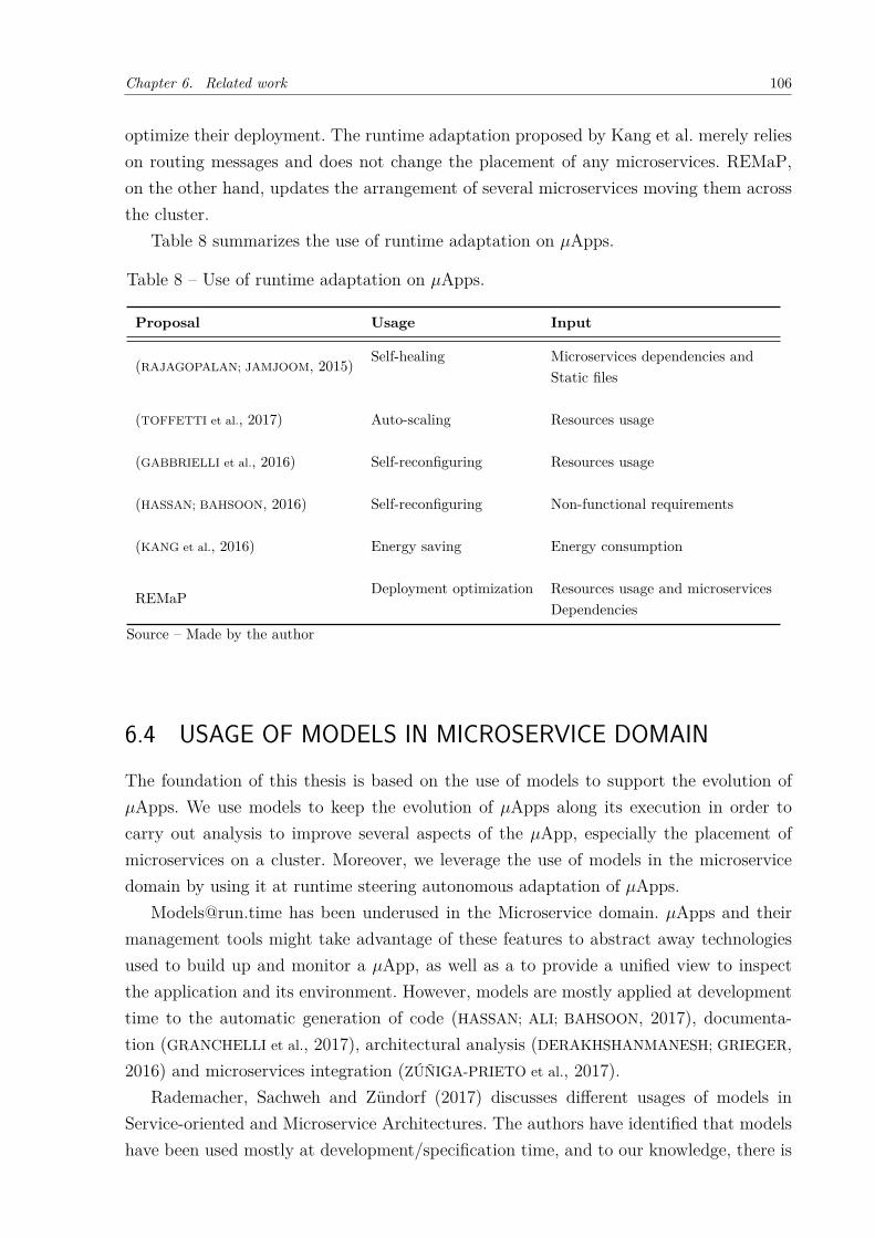
Chapter 6. Related work 106

optimize their deployment. The runtime adaptation proposed by Kang et al. merely relieson routing messages and does not change the placement of any microservices. REMaP,on the other hand, updates the arrangement of several microservices moving them acrossthe cluster.

Table 8 summarizes the use of runtime adaptation on 𝜇Apps.

Table 8 – Use of runtime adaptation on 𝜇Apps.

Proposal Usage Input

(RAJAGOPALAN; JAMJOOM, 2015) Self-healing Microservices dependencies andStatic files

(TOFFETTI et al., 2017) Auto-scaling Resources usage

(GABBRIELLI et al., 2016) Self-reconfiguring Resources usage

(HASSAN; BAHSOON, 2016) Self-reconfiguring Non-functional requirements

(KANG et al., 2016) Energy saving Energy consumption

REMaP Deployment optimization Resources usage and microservicesDependencies

Source – Made by the author

6.4 USAGE OF MODELS IN MICROSERVICE DOMAINThe foundation of this thesis is based on the use of models to support the evolution of𝜇Apps. We use models to keep the evolution of 𝜇Apps along its execution in order tocarry out analysis to improve several aspects of the 𝜇App, especially the placement ofmicroservices on a cluster. Moreover, we leverage the use of models in the microservicedomain by using it at runtime steering autonomous adaptation of 𝜇Apps.

Models@run.time has been underused in the Microservice domain. 𝜇Apps and theirmanagement tools might take advantage of these features to abstract away technologiesused to build up and monitor a 𝜇App, as well as a to provide a unified view to inspectthe application and its environment. However, models are mostly applied at developmenttime to the automatic generation of code (HASSAN; ALI; BAHSOON, 2017), documenta-tion (GRANCHELLI et al., 2017), architectural analysis (DERAKHSHANMANESH; GRIEGER,2016) and microservices integration (ZÚÑIGA-PRIETO et al., 2017).

Rademacher, Sachweh and Zündorf (2017) discusses different usages of models inService-oriented and Microservice Architectures. The authors have identified that modelshave been used mostly at development/specification time, and to our knowledge, there is

Chapter 6. Related work 107

no work using models at runtime in the microservice domain. Despite the lack of works ofmodels at runtime for microservices, Rademacher, Sorgalla and Sachweh (2018) show thechallenges in decomposing monolith applications into 𝜇Apps. They claim that Domain-driven design (DDD) provides modeling means for software design to decompose domainsin bounded contexts. Thereby, each identified into a monolith (context cluster) denotesa candidate for a microservice. However, the authors suggest that models are typicallyunder-specified, which poses several challenges when applying a domain driven design tocreate the 𝜇Apps. Finally, they presented selected tools of model-driven development tocope with such problems.

Development support. Most of the works on models for 𝜇Apps aim to supportthe development of applications and offline tasks such as static analysis for architecturalevolution (HASSAN; ALI; BAHSOON, 2017) and support for deployment (LEITNER; CITO;

STÖCKLI, 2016).Derakhshanmanesh and Grieger (2016) identifies how models might be used across the

full software lifecycle, including runtime, to evolve the application. Derakhshanmaneshand Grieger proposes the usage of a domain-specific modelling language (DSML) andmodel transformations to define and evolve a microservice application at the architecturallevel.

Rademacher, Sachweh and Zündorf (2018) presents a model for creating 𝜇Apps. Theconcepts adopted in this model are deduced from existing approaches to SOA modelling.Moreover, it adds frequent concepts from 𝜇Apps, such as API gateways. The model wasstructured in different viewpoints like in REMaP. However, their viewpoints comprise thedata, services, and operations of a 𝜇App wheras REMaP comprises different abstractionsof a 𝜇App, such as nodes, applications and microservices.

Hassan, Ali and Bahsoon (2017) proposes a mechanism, named Microservice Ambients,to support the evolution of monolithic architectures for microservices at development time.

Leitner, Cito and Stöckli (2016) present an approach for model deployment cost. Themodel is generated by analyzing messages exchanged among microservices and creatinga direct acyclic graph (DAG). The proposed algorithm, namely CostHat, is applied tothe graph in order to calculate the costs generated by IO, compute, API calls, and otherconstant cost factors in a 𝜇App.

Code generation. Among all offline tasks supported by models, code generation isthe most used. Düllmann and Hoorn (2017) have used models for engineering microservicetestbeds. The model is created by developers and generates Java code and deploymentfiles (Maven, Docker, and Kubernetes). The microservices generated are automaticallyinstrumented to collect metrics at runtime.

MicroArt (GRANCHELLI et al., 2017) is a tool to perform static and dynamic analysisof code repository and microservice environment (Docker). These analyses are guided bya software architect and create an architectural model of the application. The model is

Chapter 6. Related work 108

used to show the application graph, the development team and the cluster where theapplication is deployed. Nothing about runtime metrics and messages are represented inthis model. Also, this model is not used at runtime.

Sorgalla et al. (2018) proposes a collaborative model for development teams creating𝜇Apps. The model is a first-class citizen on development, not restricted only for specifica-tion but being used to generate code and integrate microservices. However, the proposedmodel does not update/upgrade the 𝜇App at runtime autonomously.

Integration. Usually, the code generation is carried out to integrate microservicesautomatically. Zúñiga-Prieto et al. (2017) propose a model, inspired on SoaML (OMG,2012), to integrate microservices. Developers should specify the integration, describing theintegration logic and architectural impact of integration without taking into considerationthe particularities of any cloud environment. In the end, the model is used to generateskeletons of microservices, the integration logic and scripts to automatically deploy andintegrate the microservices.

Sorgalla (2017) presents AjiL, a domain-specific modeling language (DSML) to create𝜇Apps. The language aims to reduce the complexity of the creation of 𝜇Apps by ab-stracting development and integration technologies in microservices. AjiL is a graphicallanguage that facilitates the creation of applications by business experts.

Thramboulidis, Vachtsevanou and Solanos (2018) proposes a framework to build cyber-physical 𝜇Apps by using models. Like REMaP, this approach uses a model to abstract theheterogeneity of the entities that compose the system. In this case, a manufacturing plantof industry 4.0 (LASI et al., 2014). Their platform abstracts these elements and developersthen use the model to integrate the elements in the plant detached of their technology.Unlike REMaP, the model is not used for runtime adaptation of the system.

Table 9 highlights the primary usage of these works and compare them with REMaP.

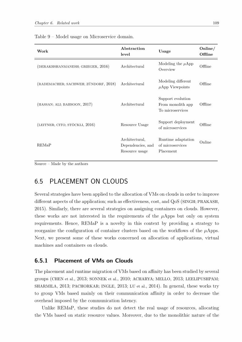
Chapter 6. Related work 109

Table 9 – Model usage on Microservice domain.

Work Abstraction Usage Online/level Offline

(DERAKHSHANMANESH; GRIEGER, 2016) Architectural Modeling the 𝜇App OfflineOverview

(RADEMACHER; SACHWEH; ZÜNDORF, 2018) Architectural Modeling different Offline𝜇App Viewpoints

(HASSAN; ALI; BAHSOON, 2017) ArchitecturalSupport evolution

OfflineFrom monolith appTo microservices

(LEITNER; CITO; STÖCKLI, 2016) Resource Usage Support deployment Offlineof microservices

REMaPArchitectural, Runtime adaptation OnlineDependencies, and of microservicesResource usage Placement

Source – Made by the authors

6.5 PLACEMENT ON CLOUDSSeveral strategies have been applied to the allocation of VMs on clouds in order to improvedifferent aspects of the application; such as effectiveness, cost, and QoS (SINGH; PRAKASH,2015). Similarly, there are several strategies on assigning containers on clouds. However,these works are not interested in the requirements of the 𝜇Apps but only on systemrequirements. Hence, REMaP is a novelty in this context by providing a strategy toreorganize the configuration of container clusters based on the workflows of the 𝜇Apps.Next, we present some of these works concerned on allocation of applications, virtualmachines and containers on clouds.

6.5.1 Placement of VMs on Clouds

The placement and runtime migration of VMs based on affinity has been studied by severalgroups (CHEN et al., 2013; SONNEK et al., 2010; ACHARYA; MELLO, 2013; LEELIPUSHPAM;

SHARMILA, 2013; PACHORKAR; INGLE, 2013; LU et al., 2014). In general, these works tryto group VMs based mainly on their communication affinity in order to decrease theoverhead imposed by the communication latency.

Unlike REMaP, these studies do not detect the real usage of resources, allocatingthe VMs based on static resource values. Moreover, due to the monolithic nature of the

Chapter 6. Related work 110

applications deployed in VMs, it is not common to reconfigure the VM placement in orderto improve application requirements since the monolithic application is not as dynamicas a 𝜇App.

Close to our work, Bayless et al. (2017) uses MonoSat, a SMT solver specialized inflow problems. MonoSat optimizes the deployment of virtual clusters, based on VMsand node resources, network bandwidth and requirements of the virtual cluster. UnlikeREMaP, the main problem solved by the authors is to maximize the flow of data andnot the co-location of services (VMs or containers) into the cluster. The specialization ofMonoSat for network flows allowed the achievement of relevant results in comparisonto other SAT solvers. However, the features of MonoSat are not useful for bin-packproblem variants like ours, which lead us to use general purpose SAT solvers that are notgood for handling the optimization of large cluster allocations.

Finally, in addition to the affinity based on communication, other kinds of relationshipshave been explored. Some examples are data affinity (JIANG et al., 2017) – which tries todeploy the application close to the data being used – and feature affinity (RAMAKRISHNAN

et al., 2013), in which the application is disposed of according to available host features.

6.5.2 Placement of Containers on Clouds

Existing proposals related to the placement of microservices are not concerned with theruntime behaviour (workflow) of the 𝜇App. None of them try to automatically detectthe behaviour of the 𝜇Apps (workflow) in order to reconfigure the placement of theirmicroservices at runtime.

Reducing monetary cost. JRO (GABBRIELLI et al., 2016) uses static resource values,set by users, to deploy microservices on the cluster, similar to commercial approaches suchas Kubernetes and Docker Swarm.

The user sets the requirements of CPU and memory usage, the number of replicasand the dependencies between the microservices. JRO uses this information, with data ofVMs in the cluster – monetary cost, memory and CPU – to calculate the deployment of𝜇Apps minimizing the cost and satisfying the 𝜇Apps needs.

Both JRO and REMaP use a multi-objective optimization strategy to place microser-vices in a cluster. However, JRO is not concerned with changing the 𝜇App at runtimebased on its behaviour. REMaP on the other hand continuously monitors the 𝜇App andreconfigures its placement whenever affinities between microservices change.

Improvement in resource usage. Medel et al. (2017) propose a new Kubernetesscheduler in order to place containers on the cluster based on containers characterization –e.g., the application into the container is CPU or I/O bounded, defined by the developers.The characterization allows the scheduler to evaluate what is the best configuration todeal with the workload at a given moment.

Chapter 6. Related work 111

The authors use the characterization of the applications according to to the resourcesthey use more intensively – CPU, I/O disk, network bandwidth or memory. The charac-terization is made manually by the application owner, and the scheduler uses this charac-terization to place containers on the cluster. Medel et al. developed a schedule to balancethe number of applications in each node; and/or to minimize the degradation in a machinecaused by resource competition.

Medel et al. also considers that the mechanism provided by management tools, likeKubernetes and Docker Swarm, are insufficient to deal with the placement of containers(microservices). The authors use an approach similar to ours and aim to detect resourcecontention of microservices and decide where to place them. However, REMaP is a fullyautomatized tool and can change the configuration at runtime according to the 𝜇App’sbehaviour changes. The scheduler proposed by Medel et al. only acts on the deploymentphase of the application or when the microservice scales out. Moreover, they are notinterested in using the interaction between microservices as the input of their scheduler.

Awada and Barker (2017) analyzes the container resource usage in order to group themand avoid resource contention – improving the overall performance of the applications.

The authors aim to optimize cluster resource utilization and minimize the overallexecution time of tasks on clouds in different geographical regions. The approach consid-ers requirements of containerized applications in order to achieve high throughput, highresource utilization and faster execution time. Awada and Barker’s approach captureshigh-level resource requirements to get an updated state of multi-region cloud cluster forresource availability. Then, they merge the container representation to form new multi-container units and deploy these units on container-instances.

The approach presented by Awada and Barker has some similarities to REMaP. Inboth cases, the solution aims to improve the performance of 𝜇Apps, decrease resourceusage and avoid resource contention. However, Awada and Barker are not interested inusing the runtime behaviour of 𝜇Apps to update the placement of their microservices onthe fly.

Kaewkasi and Chuenmuneewong (2017) uses a meta-heuristic algorithm, named AntColony Optimization (ACO), to improve the scheduler’s optimality. The proposed al-gorithm spreads the application throughout containers in order to balance the overallresource usage better and lead applications to better performance in comparison to thedefault management tool algorithms.

The proposed algorithm helps to maximize the application performance rather thancontainers being fully packed into a single node. For each iteration, the algorithm triesto put tasks onto available resources in such way that it reduces the total amount ofresources being used.

Filip et al. (2018) propose a scheduling algorithm for allocating microservices in aNano Data Center (VALANCIUS et al., 2009). This approach uses primitive microservices

Chapter 6. Related work 112

to compose tasks for processing a given data.The scheduling algorithm considers a previous analysis of resource consumption of

each task and analyzes the available resources currently in the cluster, aiming a balanceddistribution of the tasks in the cluster. It also considers the monetary cost of the ex-ecution. First, the mechanism knows beforehand how many steps are necessary for themicroservice to be executed and calculates the estimated time to perform a task. Based onthe resources available in the Nano Data Centers (NaDa), the microservices are allocatedto the “servers” on the edge of the network (e.g., gateways and cable modems) based ontheir resources availability.

The idea proposed by Filip et al. aims to schedule IoT microservices on NaDa and notconsider the affinities between microservices to co-locate them in a NaDa. Despite thesimilarities – e.g., considering previous analysis during scheduling – the REMaP proposalis for common 𝜇Apps.

(ADAM; LEE; ZOMAYA, 2017) uses a stochastic approach in order to avoid over-provisioningthe resources on a cluster. Their mechanism promotes auto-scaling of microservices byapplying their algorithm, named Two-stage Stochastic Programming Resource Allocator(2SPRA), on metrics such as network latency and CPU utilization.

Reduce energy consumption.GenPack (HAVET et al., 2017) uses an approachsimilar to garbage collectors to partition the cluster into groups of machines for differ-ent containers lifetime. According to resource usage and lifetime, containers are smartlyscheduled to specific groups – co-locating containers with complementary resource re-quirements. The objective of GenPack is to decrease the energy consumption by thecluster.

GenPack does not know the properties of containers and workloads in advance –it relies on runtime monitoring to observe the resource usage of containers while in a“nursery”. Containers run in a young generation of servers which hold short-running jobsand experience relatively high turnaround. This region is like the heap memory space ina garbage collector. Long-running jobs are migrated to the old generation, composed ofmore stable and energy efficient servers. GenPack runs on top of Docker Swarm.

GenPack uses meta-heuristic is based on genetic algorithms to schedule containersin the cluster. This approach does not use the communication between microservices todecide about their allocation. However, similarly to REMaP, GenPack moves microser-vices at runtime across different regions of the cluster. These movements are performedaccording to the generation of the microservices.

Reduce network impact. Guerrero, Lera and Juiz (2018) propose the use of a non-dominated sorting genetic algorithm-II (NSGA-II) to schedule microservices (containers)on a cluster.

The authors aim to achieve equal distribution of the workload along container repli-cas and physical machines; reduction of network overheads and better reliability. This

Chapter 6. Related work 113

approach has a superior performance than Kubernetes plain-scheduler. Furthermore, thisapproach uses a smaller number of physical machines than Kubernetes, with improve-ment ratios of up to 4.8 times faster than Kubernetes. However, they are not interestedin improving the performance of 𝜇Apps at all.

Unlike REMaP, Guerrero, Lera and Juiz are neither interested in handling resourcecontention problems nor improving 𝜇App performance by moving the microservices atruntime.

(BHAMARE et al., 2017) uses an affinity-based approach to schedule microservicesin a multi-cloud scenario to decrease the traffic, generated by microservices, and theturnaround to time in order to deliver service to costumers. Unlike REMaP, this ap-proach is neither concerned about resource contention at runtime nor in adapting theplacement of microservices at runtime – due to different workflows that may come upduring the 𝜇App execution.

In our approach, we are not concerned in an optimized auto-scaling – we aim tooptimize the placement of 𝜇Apps after the calculation of an auto-scaling.

Like REMaP, all those approaches agree about the need to monitor and analyze run-time aspects of the microservices and containers in order to better allocate them in thecluster. However, none of them try to optimize the placement of microservices based onchanges in 𝜇App behaviour. They also do not consider the relationship of microservices(containers) and the 𝜇App workflow to co-locate them in order to improve the overallperformance of the 𝜇App.

Table 10 summarize the strategies for smart placement of microservices (containers)in the cloud.

6.5.3 Allocation in High-Performance Computing

In high-performance computing (HPC), there are several affinity-based strategies to al-locate jobs (processes, VMs or containers). The most common approaches compute theaffinity of jobs and raw resources (e.g., CPU, GPU, I/O), and are not focused on inter jobs.For instance, Lee and Katz (2011) calculate the affinities between resources and jobs insuch a way that an affinity is a metric of how much a resource contributes to the executionof a job. Yokoyama et al. (2017) calculating the affinity based on how much competitionexists between jobs for a given resource. More sophisticated affinities may consider aninter-process relationship to allocate processes to the same virtual CPU and/or virtualCPUs to the same physical CPU, avoiding cache misses along the application execution(LI et al., 2010). In all cases, the allocation is on the process and CPU levels, at a lowerlevel than REMaP.

There are works in which affinities are calculates based on job communication, likeREMaP. AAGA (CHEN et al., 2013), CIVSched (GUAN et al., 2014), and Starling (SONNEK

et al., 2010) are some examples of this approach. In general, these works compute the

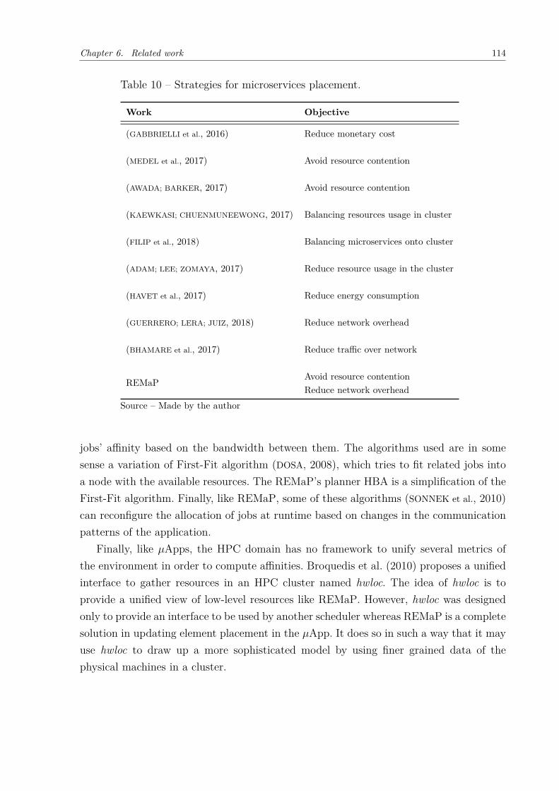
Chapter 6. Related work 114

Table 10 – Strategies for microservices placement.

Work Objective

(GABBRIELLI et al., 2016) Reduce monetary cost

(MEDEL et al., 2017) Avoid resource contention

(AWADA; BARKER, 2017) Avoid resource contention

(KAEWKASI; CHUENMUNEEWONG, 2017) Balancing resources usage in cluster

(FILIP et al., 2018) Balancing microservices onto cluster

(ADAM; LEE; ZOMAYA, 2017) Reduce resource usage in the cluster

(HAVET et al., 2017) Reduce energy consumption

(GUERRERO; LERA; JUIZ, 2018) Reduce network overhead

(BHAMARE et al., 2017) Reduce traffic over network

REMaP Avoid resource contentionReduce network overhead

Source – Made by the author

jobs’ affinity based on the bandwidth between them. The algorithms used are in somesense a variation of First-Fit algorithm (DOSA, 2008), which tries to fit related jobs intoa node with the available resources. The REMaP’s planner HBA is a simplification of theFirst-Fit algorithm. Finally, like REMaP, some of these algorithms (SONNEK et al., 2010)can reconfigure the allocation of jobs at runtime based on changes in the communicationpatterns of the application.

Finally, like 𝜇Apps, the HPC domain has no framework to unify several metrics ofthe environment in order to compute affinities. Broquedis et al. (2010) proposes a unifiedinterface to gather resources in an HPC cluster named hwloc. The idea of hwloc is toprovide a unified view of low-level resources like REMaP. However, hwloc was designedonly to provide an interface to be used by another scheduler whereas REMaP is a completesolution in updating element placement in the 𝜇App. It does so in such a way that it mayuse hwloc to draw up a more sophisticated model by using finer grained data of thephysical machines in a cluster.

Chapter 6. Related work 115

6.6 CONCLUDING REMARKSIn this chapter we positioned our work on state-of-the-art runtime adaptation of microser-vices. The runtime adaptation of microservices is related to the concepts of microserviceevolution and placement of microservices on cloud. We position our work in relation tothese subjects. Moreover, REMaP uses Models@run.time to support the adaptation of𝜇Apps. Hence, we position our work in relation to the use of models on microservices andservices adaptation.

116

7 CONCLUSION AND FUTURE WORK

This chapter presents the conclusion and next steps of this thesis. We show the potentialof REMaP for: improving the performance, reducing resource waste and reducing theresource contention of 𝜇Apps in a cluster. We highlight our contributions on using Mod-els@run.time for 𝜇Apps and runtime placement of 𝜇Apps as well as discuss the limitationsof our approach. Finally, we present future directions of this research.

7.1 CONCLUSIONDespite the flexibility provided by microservices, existing management tools cannot applyrich adaptations to 𝜇Apps at runtime. To enrich how the adaptation is carried out on a𝜇App, we propose a platform-independent runtime adaptation mechanism to reconfigurethe placement of microservices based on their communication affinities and runtime re-sources usage. To achieve it, we developed REMaP (RuntimE Microservices Placement),an adaptation manager that monitors the 𝜇App and uses collected data to reorganize theplacement of the microservices.

At the core of our approach is a innovative optimization that changes the arrangementof microservices at runtime. REMaP is our view on how Models@run.time drives theadaptation of a 𝜇App. Hence, in this work, we use a model to provide a unified view ofthe 𝜇App and to ensure safe changes to the 𝜇App.

The model abstracts several technologies involved in the cluster and 𝜇App monitoring,organizing all data collected into a unified structure – providing a single view of the𝜇App. The model also highlights different aspects of the 𝜇Apps, such as 𝜇App workflowand topology, and allow the inference of new information about the 𝜇App. Moreover, theadaptation manager uses the model during 𝜇App adaptation to ensure that the adaptationwill not lead the 𝜇App to an inconsistent configuration. All adaptations are first checkedon model for this, if they are safe, they are applied to the application.

REMaP is based on the MAPE-K architecture, which defines four phases to managesystems autonomously. These phases are monitoring, analysis, planning and execution.There is a knowledge-base, used to maintain useful information for the adaptation process,weaved to each phase.

In the monitoring phase, REMaP collects heterogeneous data, such as metrics andcommunication messages, from several sources and unifies them into a model. REMaPuses this model as a knowledge-base throughout the other phases of MAPE-K.

During the analysis phase, REMaP inspects the model looking for affinities betweenthe microservices. An affinity defines a degree of relationship between two microservicesand is calculated based on the number as well as size of messages exchanged. REMaP uses

Chapter 7. Conclusion and Future Work 117

the affinities in the planning phase. The adaptation is calculated based on: the affinities,records of resource usage and resources available in the cluster. The objective of theadaptation is to co-locate microservices with high affinity using the resource usage andresources available as constraints.

Once the adaptation is calculated, REMaP executes it by collocating high relatedmicroservices. The adaptation process is guided by the model, that maintains a causalconnection with the 𝜇App and avoids inconsistencies between the adaptation to be appliedand the current state of the application.

In the end, the adaptation process has potential to:

1. Improve the 𝜇App performance: Co-locating high related microservices decreasesthe network impact on the microservice’s communication, improving the overallperformance of the 𝜇App;

2. Reduce resource wasting: Co-locating lightweight microservices avoids their execu-tion in individual hosts; and

3. Reducing resource contention: Co-locating microservices based on their previous re-source consumption avoids them being put together with heavyweight microservices.While peaks are difficult to be identified by gathering the current resource usage,information about historical resource consumption allows REMaP a better view ofthe behaviour of the 𝜇App.

Finally, 𝜇Apps are dynamic applications and continually change their behaviour (work-flows). The dynamic performance makes the affinities vary along the 𝜇App execution. Un-like existing approaches, whose scheduling is performed only when the application startsto execute, REMaP continuously observes the 𝜇App’s behaviour – adapting its placementwhenever necessary, according to the new affinities that arise at runtime and changes inresource usage history.

7.2 SUMMARY OF CONTRIBUTIONSThe main contribution of this thesis the management of 𝜇Apps by promoting adaptationdriven by Models@run.time which unify different behavioral aspects of the application. Weachieved this contribution through:

1. The definition of a service evolution model and its use at runtime to support themanagement of 𝜇Apps by abstracting the heterogeneity of 𝜇App environments andorganizing concepts related to microservice domain; and,

2. The characterization and use of the affinity concept between microservices in orderto dynamically change their placement.

Chapter 7. Conclusion and Future Work 118

Next, we discuss the contribution highlighting these two aspects studied as well as thesecondary contributions that come up along the development of this thesis.

7.2.1 Service evolution model for 𝜇Apps

REMaP makes intensive use of Models@run.time. We contributed by proposing a servicesevolution model – flexible to several situations in the management of 𝜇Apps– to describe𝜇Apps. In this thesis, we presented several circumstances where the model can be usedand how we vary the initial version of the services evolution model to be used in ourruntime adaptation manager.

𝜇App management is a cumbersome task performed by 𝜇App engineers. Different toolsused in the microservice domain makes difficult a complete view of the running 𝜇App. Toachieve it, engineers must observe various aspects of the application individually, such asresource usage, communication and logs. Furthermore, a different set of non-integratedtechnologies are also used for each element.

Our contribution to this problem is to unify all the information in a Models@run.-time used to provide a complete view of the 𝜇App without taking into considerationits monitoring technology. Moreover, the use of Models@run.time makes the model inconformance with the 𝜇App throughout its execution. The causal connection between themodel and the 𝜇App in execution is essential since 𝜇Apps change several times duringtheir existence. By using a live model (Models@run.time), we can track all changes carriedout on the 𝜇App, maintaining a reliable view of its structure and behaviour.

Our solution also shows the importance and viability of using Models@run.time in themicroservice domain. In particular, the proposed model includes elements that serve tocharacterize the microservice domain and 𝜇Apps.

7.2.2 Runtime Placement of 𝜇Apps

The runtime adaptation of 𝜇Apps relies mostly on the scale in and out activities based onresource usage – with few works handling other types of runtime adaptation. Moreover,the adaptation on 𝜇Apps uses real-time metrics or static information – set by engineersto guide the adaptation. They do not look at the execution history of the 𝜇App neitherits behaviour to take any action.

Our contribution related to this subject, is to perform runtime adaptation of mi-croservice placement based on past data and behavioural information. Our proposal foranalyzing microservice data records allows adaptation managers to make reliable decisionsinstead of unsafe choices based on ephemeral data (e.g. snapshot real-time metric usage)that does not represent the whole behaviour of the system.

Moreover, our approach uses the concept of microservice affinities to reorganize theplacement of microservices. In the exploratory phase of this thesis, we observed the impact

Chapter 7. Conclusion and Future Work 119

of the placement of the 𝜇App performance. Based on this observation, we understood howwe could analyze whether microservices should be co-located or not – hence, we definedthe concept of affinity. With this concept, we can understand the behaviour of 𝜇Appsbetter and take more robust decisions by not considering only application metrics.

Our adaptation approach considers the behaviour of the 𝜇App and not only metrics,leading the decision making to be more robust and dynamic. 𝜇Apps are dynamic appli-cations and their behaviour changes many times along its execution. Performing analysison these applications by checking only “static data” such as metric snapshots providespoor feedback to the management mechanism.

Finally, the adaptation of 𝜇Apps by reorganizing the placement of microservices isa novelty in this domain. Works related to this topic statically handle the arrangement.Based on a set of information, the scheduler of management tools decides to optimizethe first deployment of the 𝜇App and, in some cases, the installation of microservicereplicas. The management tools are not aware of how runtime changes affect the 𝜇Appbehaviour and the initial placement strategy might not be useful anymore. Our approachcontinuously checks the new behaviour that comes up from a 𝜇App due to the calculationof affinities. Therefore, we can reorganize the placement of 𝜇Apps as well as the 𝜇Appchanges its behaviour.

7.2.3 Secondary Contributions

The main contributions of this thesis are substantiated in several secondary contributionsas described in the following:

Characterization of adaptation on 𝜇Apps. In the early stage of this work weinvestigated the meaning of adaptation for 𝜇Apps. During research, we elaborated andcrystallized this concept for the microservice domain – we systematized that adaptationfor 𝜇Apps stands for updates or upgrades. An update is an adaptation that changesthe arrangement of the 𝜇App in a cluster – e.g., scaling in and out or reorganizing theplacement of 𝜇Apps. Upgrade on the other hand, changes the implementation and/or theworkflow of the 𝜇App– e.g., rolling out and back microservice versions. Moreover, anyadaptation of the 𝜇App relies on instantiating microservices somewhere. Therefore, wecontribute by specializing the general concept of adaptation for the bounded domain ofmicroservices.

Heuristic to reorganize the 𝜇App placement. The problem of the optimal place-ment of 𝜇Apps is hard to solve due to its theoretical characteristics. We propose a heuristicto decide where to place high related microservices. Our algorithm is good enough for themost common scenarios evaluated in this thesis and can be reasonably used as the startingpoint for the development of more sophisticated algorithms.

Optimization model to reorganize 𝜇App placement. As an attempt to placea 𝜇App in a cluster optimally, we used the Z3 SMT solver – considering our objectives

Chapter 7. Conclusion and Future Work 120

and constraints. To our knowledge, SMT solvers are not traditionally used to solve multi-objective bin-packing problems where affinities are part of the constraints/objectives to besolved/reached. Nowadays, existing solutions only consider resource usage and availableresources as input. Therefore, we contribute by creating an optimization model for Z3that uses this new approach (metrics and affinities) to calculate an optimal placement ofmicroservices.

Framework for creating mock 𝜇Apps. The use of real 𝜇Apps to validate worksis a challenge. There are few 𝜇Apps and open source available which are similar in sizeand complexity to 𝜇Apps running real companies. Due to this limitation, we created aframework to emulate real 𝜇Apps running on a cluster managed by a Kubernetes toolby creating artificial microservices and host configurations – attaching microservices tohosts and linking the microservices make up a mock 𝜇App. We used this framework togenerate the mock instances used in our evaluation. This minor contribution is useful forother people who aim to validate their proposals in large scale if they do not have a real𝜇App to validate it.

MAPE-K based adaptation manager for 𝜇Apps. MAPE-K is the reference archi-tecture on developing tools for autonomously managed systems. In this context REMaPis a innovation as it is the first adaptation tool for 𝜇Apps that uses Models@run.time toguide the adaptation process. Existing tools only consider real-time information to reasonand act on a 𝜇App. REMaP on the other hand, can reason about past data and infer newinformation on the 𝜇Apps behaviour by using Models@run.time– making it a robust toolto manage 𝜇Apps autonomously.

7.3 THREATS OF VALIDITYNext, we list the threats of validity related to REMaP.

Evaluation on a single real-world application. REMaP was evaluated by usinga mock and an empirical approach. However, the empirical one was carried out on asingle real 𝜇App named Sock-shop. Even though Sock-shop is widely used as a reference𝜇App, it cannot pop up a wide range of situations to exercise all features of REMaPat once, thus limiting our evaluation. Moreover, the other open-sourced 𝜇Apps availableare in most cases incomplete, unstable, cumbersome or infrastructure dependent (differentcloud providers such as Amazon AWS, Google Cloud Platform, and IBM Bluemix). Thesecharacteristics make it difficult to set up an evaluation testbed – mainly because theinfrastructure dependency demands a high monetary cost in order to solve them.

Not handling replicas during the adaptation. REMaP does not cover an impor-tant aspect during the movement of microservices – handling its replicas. The migration ofa container (microservice) is not like the migration of a virtual machine, which can freezeits state and execution while it is being moved and then be resumed. Containers are

Chapter 7. Conclusion and Future Work 121

processes that exist so that there is a technological limitation to carry out the migrationof containers across different machines, like virtual machines. Due to this situation, themovement of a microservice relies on deleting its instance in the source and instantiatinga new one in the destination. This task is under the responsibility of management tool’sscheduler. Therefore, we decided not to consider replicas since it would be necessary todevelop a whole new scheduler for a management tool (e.g., Kubernetes) that was out ofthe scope of this thesis.

Adaptation based on few quality attributes. In the current implementation,REMaP computes an adaptation guided by only two quality attributes, performance andresource consumption, leaving out other important cases, such as resiliency and secu-rity. This current strategy makes REMaP unaware of important aspects of a distributedsystems, which avoid that more robust adaptations be applied on 𝜇Apps. For instance,REMaP is unaware of failures frequency of the microservices. Hence, REMaP cannot de-cide to maintain more replicas of a given microservices of avoid long downtimes in additionto place these replicas in a optimal location.

Dumb1 Monitoring. REMaP monitoring gathers data from a different data storeand uses this information to populate the model. Although 𝜇Apps are dynamic, muchinformation should be inferred based on the context of the environment (e.g., time) andhistorical data. As we are aiming to build an end-to-end solution, we do not focus on theoptimization of the process; hence we do not Implement techniques to make the monitoringsmarter – using machine learning to foresee metric usage, statistical analysis to gatherfewer amounts of data an so on. The use of these techniques could partially improve theoverall performance of REMaP by decreasing the amount of data being collected.

REMaP is not microservice-based. Microservice style promotes easy maintenanceby the developer’s teams. It is not right for a single person to maintain a complex ap-plication like REMaP. Debugging an application of an ongoing project is a hard taskand is even worse if it is distributed as the microservice style suggests. Hence, despiteREMaP using most of the architectural patterns adopted by 𝜇Apps– such as separationof concerns, well defined bounded components, asynchronous communication – its imple-mentation does not follow the technological standards suggested for 𝜇App development.

Adaptation trigger is semi-automatized. Our current implementation uses a pa-rameterized value to trigger the adaptations – the adaptation mechanism checks the 𝜇Appat pre-determined time intervals set by a 𝜇App engineer. This approach leads REMaPto become a semi-automated solution for adapting 𝜇Apps. However, to fully automatizewhen the adaptation starts, an entire work is necessary in order to systematize how muchdata is needed to sample and analyze a given aspect of the 𝜇App and then safely triggerthe adaptation. To fully automatize adaptation triggering, further study on the smart1 Not smart. For example, smartphone (e.g., iPhone) and dumbphone (e.g., old fashion cell phone - the

era before smartphones)

Chapter 7. Conclusion and Future Work 122

sampling of 𝜇App data, including the use of statistical and artificial intelligence methods,is necessary in order to reach a reliable number; however, these approaches are out of thescope of this thesis.

Using EMF to keep the Models@run.time. EMF is a widely adopted Java frame-work used in Model Driven Development (MDE) that provides much ease for modellingand handling Models@run.time. The EMF was not developed initially to be thread safe,which makes its usage in a multi-threaded application unsafe. However, due to the easeprovided by the framework, we choose it for a fast development over runtime perfor-mance. As a consequence, REMaP has a poor performance in handling the model – sinceits implementation is mostly single-threaded and, when multi-threaded, it suffers froman overhead, imposed by the use of synchronization primitives. This strategy means thatREMaP does not use all the power of its host to populate the model and calculate theaffinities. As a consequence, the model handling is a bottleneck in the adaptation process.

Non-optimized implementation of planning algorithms. Similar to the issueof processing the model in a non-optimized model, we choose to implement the planningalgorithms with minimum optimization to facilitate its development. planner OA that usesZ3, an industrial SMT solver, to calculate the adaptation. The Z3 programming modelhas a steep learning curve, which makes it difficult to master its programming model andoptimize an ongoing code simultaneously. Despite these problems, minor optimizationswere applied, such as using data types of small sizes to reduce the search space duringplanning calculation. However, it is clear that there is a possibility of employing moreoptimizations in the Z3 model, consequently improving the results obtained in this thesis.

7.4 FUTURE WORKSBased on the threats of the validity of this thesis, we present some future works that shouldbe implemented to make REMaP a robust platform of runtime adaptation in 𝜇Apps.

Supporting microservice evolution. It would be interesting to identify a set ofdesired architectural and deployment patterns and monitor their preservation as the ap-plication evolves. This monitoring can be achieved by analyzing the collected informationin services, operations, exchanged messages, networking and CPU metrics, and so on.Whenever the application integrity or service quality is under risk, our solution mightrecommend appropriate improvements – such as replacing a microservice, splitting a mi-croservice, merging a set of microservices, or moving microservices to different hosts.

Evaluation of new real-world applications. As mentioned before, REMaP wasevaluated using a single real-world 𝜇App. We intend to use REMaP with other 𝜇Appsto check its impact on the performance of other applications. However, performing thiskind of evaluation is prohibited without any sponsorship to provide a real application– used by the industry – to the faculty. Hence, we are aiming to develop a test bed

Chapter 7. Conclusion and Future Work 123

to create 𝜇Apps on demand – following an architecture set by the user. The generalidea is to expand the framework used to create the mock experiments for this work.The framework should automatically instantiate the model (graph) generated by usingcustomized microservices – dummy microservices that receive fake messages (with sizesand request rate parameterized) and return a fake answer (also parameterized). Hence,we will be able to run experiments on a high scale and in a fully controlled environment.

Handling microservices replicas during adaptation. REMaP is not able to han-dle microservice replicas properly during the adaptation due to technological limitations.To overcome this limitation, we aim to implement a new scheduler to Kubernetes, whichwill work with REMaP so that REMaP to provide feedback and vice-versa. This ap-proach will allow microservice replicas to be naturally handled by the adaptation platform(REMaP and scheduler) during an adaptation.

Smart Monitoring. We aim to trigger the adaptation without any human interven-tion, making it necessary to define how much data is required to make a safe analysis andplan an adaptation. Accordingly, the analysis phase should be expanded to also make astatistical analysis of the amount of data collected in order to decide the best time totrigger an adaptation. Furthermore, information can be foreseen based on historical data– we can use the machine’s learning to predict future resource usage based on the historyof the 𝜇App and anticipate some changes to the 𝜇App, such as auto-scaling or place-ment reconfiguration. Therefore, we are also planning to apply statistical and artificialintelligence techniques to improve the monitoring and analysis activities.

Microservice-based REMaP implementation. We intend to split REMaP intoseveral microservices to facilitate its extension, e.g., to add new analyzers and planners.This new architecture will make REMaP more powerful so that several aspects of a 𝜇Appmight be evaluated and adapted simultaneously and at runtime.

Modern tools for handling Models@run.time. Aiming to improve the perfor-mance of REMaP’s workflow to calculate an adaptation, we intend to replace the frame-work for handling Models@run.time with more recent tools used in high-performance dataanalysis.

At first glance we aim to use non-structured data stores – graph- and document-oriented databases – due to the hierarchical and graph-based features of data collected.Even related databases are candidates. The use of related data stores is interesting dueto the number of data relationships necessary to infer information based on the datacollected from 𝜇Apps.

Another alternative is to use modern and thread-safe Models@run.time frameworks,allowing multi-thread algorithms in the analysis of the model, thus improving the overallperformance in REMaP’s adaptation.

New planning strategies. The results obtained in this work show us that althoughwe have achieved the objective of bringing autonomy to 𝜇App management, some steps

Chapter 7. Conclusion and Future Work 124

must still be improved. First of all, the adaptation of 𝜇Apps by updating the microserviceplacement is an essential issue for cluster providers. However, due to the complexity of theproblem, new strategies must be applied instead of the brute force used (SMT Solver).Therefore, we should try different techniques, such as evolutionary and swarm algorithmsmetaheuristics in order to compute an optimal placement of microservices. Moreover,we aim to improve our heuristic in order to calculate a smart placement based on moreattributes than only microservice affinities and resources usage.

Handle strongly connected sub graphs over affinities pairs. We aim to extendthe adaptation strategy by improving the analysis and planner phases to find affinityhubs in 𝜇Apps (strongly connected sub graphs) than simple microservices pairs. Ourexperiments highlight that the use of hubs by approximations algorithms may producesbetter results than co-location of simple pairs.

125

BIBLIOGRAPHY

ACHARYA, S.; MELLO, D. A. D. A taxonomy of Live Virtual Machine (Vm) Migrationmechanisms in cloud computing environment. In: IEEE. ICGCE. [S.l.], 2013. p. 809–815.

ADAM, O.; LEE, Y. C.; ZOMAYA, A. Y. Stochastic resource provisioning forcontainerized multi-tier web services in clouds. TPDS, IEEE, v. 28, n. 7, p. 2060–2073,2017.

ADERALDO, C. M.; MENDONÇA, N. C.; PAHL, C.; JAMSHIDI, P. BenchmarkRequirements for Microservices Architecture Research. In: . [S.l.]: IEEE, 2017.

AWADA, U.; BARKER, A. Improving Resource Efficiency of Container-InstanceClusters on Clouds. In: . [S.l.: s.n.], 2017. p. 929–934.

BALALAIE, A.; HEYDARNOORI, A.; JAMSHIDI, P. Microservices architectureenables devops: Migration to a cloud-native architecture. IEEE Software, IEEE, v. 33,n. 3, p. 42–52, 2016.

BALALAIE, A.; HEYDARNOORI, A.; JAMSHIDI, P.; TAMBURRI, D. A.; LYNN,T. Microservices migration patterns. Software: Practice and Experience, Wiley OnlineLibrary, v. 48, n. 11, p. 2019–2042, 2018.

BARABÁSI, A.-L.; ALBERT, R. Emergence of scaling in random networks. Science,American Association for the Advancement of Science, v. 286, n. 5439, p. 509–512, 1999.

BAYLESS, S.; KODIROV, N.; BESCHASTNIKH, I.; HOOS, H. H.; HU, A. J. Scalableconstraint-based virtual data center allocation. In: AAAI PRESS. IJCAI. [S.l.], 2017. p.546–554.

BERNSTEIN, D. Containers and cloud: From lxc to docker to kubernetes. IEEE CloudComputing, IEEE, n. 3, p. 81–84, 2014.

BHAMARE, D.; SAMAKA, M.; ERBAD, A.; JAIN, R.; GUPTA, L.; CHAN, H. A.Multi-Objective Scheduling of Micro-Services for Optimal Service Function Chains. In:IEEE. ICC. [S.l.], 2017. p. 1–6.

BICHLER, M.; LIN, K.-J. Service-oriented computing. Computer, v. 39, n. 3, p. 99–101,2006.

BIERE, A.; BIERE, A.; HEULE, M.; MAAREN, H. van; WALSH, T. Handbook ofSatisfiability: Frontiers in Artificial Intelligence and Applications. Amsterdam, TheNetherlands, The Netherlands: IOS Press, 2009.

BLAIR, G.; BENCOMO, N.; FRANCE, R. B. Models@run.time. Computer, IEEE, v. 42,n. 10, 2009.

BROQUEDIS, F.; CLET-ORTEGA, J.; MOREAUD, S.; FURMENTO, N.; GOGLIN,B.; MERCIER, G.; THIBAULT, S.; NAMYST, R. hwloc: A generic framework formanaging hardware affinities in Hpc applications. In: IEEE. Parallel, Distributed andNetwork-Based Processing (PDP), 2010 18th Euromicro International Conference on.[S.l.], 2010. p. 180–186.

Bibliography 126

BROWN, A.; KAR, G.; KELLER, A. An Active Approach to Characterizing DynamicDependencies for Problem Determination in a Distributed Environment. In: IM. [S.l.:s.n.], 2001.

CARDELLINI, V.; CASALICCHIO, E.; GRASSI, V.; PRESTI, F. L.; MIRANDOLA,R. Qos-driven runtime adaptation of service oriented architectures. In: ACM. SFSE.[S.l.], 2009. p. 131–140.

CARNEIRO, C.; SCHMELMER, T. Deploying and running microservices. In:Microservices From Day One. [S.l.]: Springer, 2016. p. 151–174.

CASATI, F.; ILNICKI, S.; JIN, L.; KRISHNAMOORTHY, V.; SHAN, M.-C. Adaptiveand dynamic service composition in eFlow. In: SPRINGER. ICAISE. [S.l.], 2000. p.13–31.

CHEKURI, C.; KHANNA, S. On multidimensional packing problems. SIAM, SIAM,v. 33, n. 4, p. 837–851, 2004.

CHEN, J.; CHIEW, K.; YE, D.; ZHU, L.; CHEN, W. AAga: Affinity-aware grouping forallocation of virtual machines. In: IEEE. AINA. [S.l.], 2013. p. 235–242.

CHOTHIA, Z.; LIAGOURIS, J.; DIMITROVA, D.; ROSCOE, T. Online Reconstructionof Structural Information from Datacenter Logs. In: Eurosys. [S.l.: s.n.], 2017.

CHRISTENSEN, H. I.; KHAN, A.; POKUTTA, S.; TETALI, P. Multidimensional binpacking and other related problems: A survey. 2016.

DERAKHSHANMANESH, M.; GRIEGER, M. Model-Integrating Microservices: Avision Paper. In: Software Engineering (Workshops). [S.l.: s.n.], 2016. p. 142–147.

DOSA, G. t. n. First Fit Algorithm for Bin Packing. In: . Encyclopedia ofAlgorithms. Boston, MA: Springer US, 2008. p. 1–5. ISBN 978-3-642-27848-8.

DÜLLMANN, T. F.; HOORN, A. van. Model-driven Generation of MicroserviceArchitectures for Benchmarking Performance and Resilience Engineering Approaches.In: ICPE. [S.l.: s.n.], 2017.

ENSEL, C. Automated Generation of Dependency Models for Service Management. In:OVUA. [S.l.: s.n.], 1999.

FELTER, W.; FERREIRA, A.; RAJAMONY, R.; RUBIO, J. An updated performancecomparison of virtual machines and linux containers. In: IEEE. ISPASS. [S.l.], 2015. p.171–172.

FILIP, I. D.; POP, F.; SERBANESCU, C.; CHOI, C. Microservices Scheduling Modelover Heterogeneous Cloud-Edge Environments as Support for Iot Applications. IEEEInternet of Things Journal, p. 1–1, 2018.

FLORIO, L.; NITTO, E. D. Gru: An Approach to Introduce Decentralized AutonomicBehavior in Microservices Architectures. In: IEEE. ICAC. [S.l.], 2016. p. 357–362.

GABBRIELLI, M.; GIALLORENZO, S.; GUIDI, C.; MAURO, J.; MONTESI, F.Self-reconfiguring microservices. In: Theory and Practice of Formal Methods. [S.l.]:Springer, 2016. p. 194–210.

Bibliography 127

GARLAN, D.; CHENG, S. W.; HUANG, A. C.; SCHMERL, B.; STEENKISTE, P.Rainbow: Architecture-based self-adaptation with reusable infrastructure. Computer,v. 37, p. 46–54, 2004.

GRANCHELLI, G.; CARDARELLI, M.; FRANCESCO, P. D.; MALAVOLTA,I.; IOVINO, L.; SALLE, A. D. Towards Recovering the Software Architecture ofMicroservice-Based Systems. In: IEEE. ICSAW. [S.l.], 2017. p. 46–53.

GUAN, B.; WU, J.; WANG, Y.; KHAN, S. CIvsched: a communication-aware inter-Vmscheduling technique for decreased network latency between co-located Vms. IEEEtransactions on cloud computing, IEEE, n. 1, p. 1–1, 2014.

GUERRAOUI, R.; PAVLOVIC, M.; SEREDINSCHI, D.-A. Trade-offs in ReplicatedSystems. Data Engineering Bulletin, IEEE, v. 39, n. 1, p. 14–26, 2016.

GUERRERO, C.; LERA, I.; JUIZ, C. Genetic algorithm for multi-objective optimizationof container allocation in cloud architecture. Journal of Grid Computing, Springer, v. 16,n. 1, p. 113–135, 2018.

HANNAFORD, J. What happens when ... Kubernetes edition! 2017.Https://github.com/jamiehannaford/what-happens-when-k8s. Online; accessed 15June 2018.

HASSAN, S.; ALI, N.; BAHSOON, R. Microservice Ambients: An ArchitecturalMeta-modelling Approach for Microservice Granularity. In: IEEE. ICSA. [S.l.], 2017. p.1–10.

HASSAN, S.; BAHSOON, R. Microservices and their design trade-offs: A self-adaptiveroadmap. In: IEEE. SCC. [S.l.], 2016. p. 813–818.

HAVET, A.; SCHIAVONI, V.; FELBER, P.; COLMANT, M.; ROUVOY, R.; FETZER,C. GEnpAck: A generational scheduler for cloud data centers. IC2E, p. 95–104, 2017.

HEORHIADI, V.; RAJAGOPALAN, S.; JAMJOOM, H.; REITER, M. K.; SEKAR, V.Gremlin: Systematic Resilience Testing of Microservices. In: ICDCS. [S.l.: s.n.], 2016. p.57–66.

HOFF, T. Microservices - Not a free lunch. 2014.Http://highscalability.com/blog/2014/4/8/microservices-not-a-free-lunch.html.Online; accessed 21 December 2017.

HOSEK, P.; CADAR, C. Safe Software Updates via Multi-version Execution. In: ICSE.[S.l.: s.n.], 2013.

HUEBSCHER, M. C.; MCCANN, J. A. A survey of autonomic computing—degrees,models, and applications. ACM Computing Surveys, v. 40, n. 3, p. 1–28, aug 2008.

IBM. An architectural blueprint for autonomic computing. [S.l.], 2005. 34 p.

JAMSHIDI, P.; PAHL, C.; MENDONÇA, N. C.; LEWIS, J.; TILKOV, S. Microservices:The Journey So Far and Challenges Ahead. Software, IEEE, v. 35, n. 3, p. 24–35, 2018.

JI, Z.-l.; LIU, Y. A dynamic deployment method of micro service oriented to Sla. IJCS,v. 13, n. 6, p. 8–14, 2016.

Bibliography 128

JIANG, J.; SUN, S.; SEKAR, V.; ZHANG, H. Pytheas: Enabling Data-Driven Qualityof Experience Optimization Using Group-Based Exploration-Exploitation. In: NSDI.[S.l.: s.n.], 2017. p. 393–406.

JORDAN, D.; EVDEMON, J. Web Services Business Process Execution LanguageVersion 2.0. 2007. Https://docs.oasis-open.org/wsbpel/2.0/wsbpel-v2.0.html. Online;accessed March 2018.

KAEWKASI, C.; CHUENMUNEEWONG, K. Improvement of container scheduling forDocker using Ant Colony Optimization. In: 254–259. [S.l.: s.n.], 2017.

KANG, D.-K.; CHOI, G.-B.; KIM, S.-H.; HWANG, I.-S.; YOUN, C.-H. Workload-awareresource management for energy efficient heterogeneous docker containers. In: IEEE.TENCO. [S.l.], 2016. p. 2428–2431.

KARASTOYANOVA, D.; HOUSPANOSSIAN, A.; CILIA, M.; LEYMANN, F.;BUCHMANN, A. Extending BpeL for run time adaptability. In: IEEE. EDOC. [S.l.],2005. p. 15–26.

KAUFMAN, L.; ROUSSEEUW, P. Clustering by means of medoids. [S.l.]: North-Holland,1987.

KELING, D.; DALMAU, M.; ROOSE, P. A survey of Adaptation Systems. IJIDCS,v. 1, n. 1, p. 1–18, 2012.

KEPHART, J. O.; CHESS, D. M. The vision of autonomic computing. Computer, v. 36,n. 1, p. 41–50, Jan 2003.

KICZALES, G.; RIVIERES, J. D.; BOBROW, D. G. The art of the metaobject protocol.[S.l.]: MIT press, 1991.

KILLALEA, T. The hidden dividends of microservices. Communications, ACM, v. 59,n. 8, p. 42–45, jul 2016.

KORTE, B.; VYGEN, J. Bin-Packing. In: . Combinatorial Optimization: Theoryand Algorithms. [S.l.]: Springer Berlin Heidelberg, 2006. p. 426–441.

KRUPITZER, C.; ROTH, F. M.; VANSYCKEL, S.; SCHIELE, G.; BECKER, C. Asurvey on engineering approaches for self-adaptive systems. PMC, Elsevier B.V., v. 17,p. 184–206, 2014.

LASI, H.; FETTKE, P.; KEMPER, H.-G.; FELD, T.; HOFFMANN, M. Industry 4.0.BISE, Springer, v. 6, n. 4, p. 239–242, 2014.

LEE, G.; KATZ, R. H. Heterogeneity-Aware Resource Allocation and Scheduling in theCloud. In: HotCloud. [S.l.: s.n.], 2011.

LEELIPUSHPAM, P. G. J.; SHARMILA, J. Live Vm migration techniques in cloudenvironment—a survey. In: IEEE. ICT. [S.l.], 2013. p. 408–413.

LEITNER, P.; CITO, J.; STÖCKLI, E. Modelling and Managing Deployment Costs ofMicroservice-based Cloud Applications. In: UCC. [S.l.: s.n.], 2016.

Bibliography 129

LEWIS, J.; FOWLER, M. Microservices. 2014.Https://martinfowler.com/articles/microservices.html. Online; accessed 21 December2017.

LI, Z.; BAI, Y.; ZHANG, H.; MA, Y. Affinity-aware dynamic pinning scheduling forvirtual machines. In: IEEE. Cloud Computing Technology and Science (CloudCom),2010 IEEE Second International Conference on. [S.l.], 2010. p. 242–249.

LU, T.; STUART, M.; TANG, K.; HE, X. Clique migration: Affinity grouping of virtualmachines for inter-cloud live migration. In: IEEE. NAS. [S.l.], 2014. p. 216–225.

MA, X.; BARESI, L.; GHEZZI, C.; MANNA, V. P. L.; LU, J. Version-consistentDynamic Reconfiguration of Component-based Distributed Systems. In: ESEC/FSE.[S.l.: s.n.], 2011.

MA, Y.; LIU, X.; WU, Y.; GRACE, P. Model-based management of service composition.In: IEEE. SOSE. [S.l.], 2013. p. 103–112.

MAES, P. Concepts and experiments in computational reflection. SIGPLAN, ACM,v. 22, n. 12, p. 147–155, dec 1987.

MEDEL, V.; TOLÓN, C.; ARRONATEGUI, U.; TOLOSANA-CALASANZ, R.;BAÑARES, J. Á.; RANA, O. F. Client-Side Scheduling Based on ApplicationCharacterization on Kubernetes. In: PHAM, C.; ALTMANN, J.; BAÑARES, J. Á.(Ed.). EGCSS. Cham: Springer International Publishing, 2017. p. 162–176.

NEWMAN, S. Building Microservices. [S.l.]: O'Reilly Media, Inc., 2015. 280 p.

NGUYEN, T.; COLMAN, A. A feature-oriented approach for web service customization.In: IEEE. Web Services (ICWS), 2010 IEEE International Conference on. [S.l.], 2010. p.393–400.

NÚÑEZ-VALDEZ, E. R.; GARCÍA-DÍAZ, V.; LOVELLE, J. M. C.; ACHAERANDIO,Y. S.; GONZÁLEZ-CRESPO, R. A model-driven approach to generate and deployvideogames on multiple platforms. JAIHC, Springer, v. 8, n. 3, p. 435–447, 2017.

OASIS. Reference Model for Service Oriented Architecture 1.0. 2006. Http://docs.oasis-open.org/soa-rm/v1.0/. Online; accessed May 2018.

OLINER, A.; GANAPATHI, A.; XU, W. Advances and Challenges in Log Analysis.CACM, v. 55, n. 2, p. 55–61, feb 2012.

OMG. Service Oriented Architecture Modeling Language Specification. 2012.Https://www.omg.org/spec/SoaML/. Online; accessed May 2018.

OREIZY, P.; MEDVIDOVIC, N.; TAYLOR, R. N. Runtime software adaptation:framework, approaches, and styles. In: ACM. ICSE. [S.l.], 2008. p. 899–910.

PACHORKAR, N.; INGLE, R. Multi-dimensional affinity aware Vm placement algorithmin cloud computing. IJACR, International Journal of Advanced Computer Research,v. 3, n. 4, p. 121, 2013.

PANDA, A.; SAGIV, M.; SHENKER, S. Verification in the Age of Microservices. In:HotOS. [S.l.: s.n.], 2017.

Bibliography 130

PAPAZOGLOU, M. P. Service -oriented computing: Concepts, characteristics anddirections. WISE, p. 3–12, 2003.

PARVIAINEN, P.; TAKALO, J.; TEPPOLA, S.; TIHINEN, M. Model-drivendevelopment processes and practices. VTT Technical Research Centre of Finland, 2009.

PEREIRA, R.; COUTO, M.; RIBEIRO, F.; RUA, R.; CUNHA, J.; FERNANDES,J. P.; SARAIVA, J. Energy Efficiency Across Programming Languages: How Do Energy,Time, and Memory Relate? In: Proceedings of the 10th ACM SIGPLAN InternationalConference on Software Language Engineering. New York, NY, USA: ACM, 2017. (SLE2017), p. 256–267. ISBN 978-1-4503-5525-4.

RADEMACHER, F.; SACHWEH, S.; ZÜNDORF, A. Differences between Model-DrivenDevelopment of Service-Oriented and Microservice Architecture. In: ICSAW. [S.l.: s.n.],2017. p. 38–45.

RADEMACHER, F.; SACHWEH, S.; ZÜNDORF, A. Analysis of Service-orientedModeling Approaches for Viewpoint-specific Model-driven Development of MicroserviceArchitecture. arXiv preprint arXiv:1804.09946, 2018.

RADEMACHER, F.; SORGALLA, J.; SACHWEH, S. Challenges of domain-drivenmicroservice design: A model-driven perspective. Software, IEEE, v. 35, n. 3, p. 36–43,2018.

RAJAGOPALAN, S.; JAMJOOM, H. App-Bisect: autonomous healing for microservice-based apps. In: USENIX ASSOCIATION. HotCLoud. [S.l.], 2015.

RAMAKRISHNAN, A.; NAQVI, S. N. Z.; BHATTI, Z. W.; PREUVENEERS, D.;BERBERS, Y. Learning deployment trade-offs for self-optimization of Internet of Thingsapplications. In: ACM. ICAC. [S.l.], 2013. p. 213–224.

SALEHIE, M.; TAHVILDARI, L. Self-adaptive software: Landscape and researchchallenges. TAAS, v. 4, n. 2, p. 1–42, 2009.

SAMPAIO JR., A.; KADIYALA, H.; HU, B.; STEINBACHER, J.; ERWIN, T.; ROSA,N.; BESCHASTNIKH, I.; RUBIN, J. Supporting evolving microservices. In: IEEE.ICSME. [S.l.], 2017.

SAMPAIO JR., A. R.; COSTA, F. M.; CLARKE, P. A model-driven Approach toDevelop and Manage Cyber-Physical Systems. In: Models@Run.time. [S.l.: s.n.], 2013. p.64–75.

SANGAL, N.; JORDAN, E.; SINHA, V.; JACKSON, D. Using Dependency Models toManage Complex Software Architecture. SIGPLAN, v. 40, n. 10, p. 167–176, 2005.

SCHMIDT, D. C. Model-driven engineering. COMPUTER, Citeseer, v. 39, n. 2, p. 25,2006.

SEO, K.-T.; HWANG, H.-S.; MOON, I.-Y.; KWON, O.-Y.; KIM, B.-J. Performancecomparison analysis of linux container and virtual machine for building cloud. ASTL,v. 66, n. 105-111, p. 2, 2014.

SINGH, A. N.; PRAKASH, S. Challenges and opportunities of resource allocation incloud computing: A survey. In: IEEE. INDIACom. [S.l.], 2015. p. 2047–2051.

Bibliography 131

SINGLETON, A. The Economics of Microservices. Cloud Computing, IEEE, v. 3, n. 5,p. 16–20, 2016.

SONNEK, J.; GREENSKY, J.; REUTIMAN, R.; CHANDRA, A. Starling: Minimizingcommunication overhead in virtualized computing platforms using decentralizedaffinity-aware migration. In: IEEE. ICPP. [S.l.], 2010. p. 228–237.

SORGALLA, J. Ajil: A graphical modeling language for the development of microservicearchitectures. In: EAM. [S.l.: s.n.], 2017.

SORGALLA, J.; RADEMACHER, F.; SACHWEH, S.; ZÜNDORF, A. On CollaborativeModel-driven Development of Microservices. arXiv preprint arXiv:1805.01176, 2018.

SZVETITS, M.; ZDUN, U. Systematic literature review of the objectives, techniques,kinds, and architectures of models at runtime. SSM, dec 2013.

TARVO, A.; SWEENEY, P. F.; MITCHELL, N.; RAJAN, V.; ARNOLD, M.; BALDINI,I. CanaryAdvisor: a statistical-based tool for canary testing (demo). In: ISSTA. [S.l.:s.n.], 2015.

THRAMBOULIDIS, K.; VACHTSEVANOU, D. C.; SOLANOS, A. Cyber-PhysicalMicroservices: An Iot-based Framework for Manufacturing Systems. arXiv preprintarXiv:1801.10340, 2018.

TOFFETTI, G.; BRUNNER, S.; BLÖCHLINGER, M.; DUDOUET, F.; EDMONDS, A.An Architecture for Self-managing Microservices. In: AIMC. [S.l.: s.n.], 2015.

TOFFETTI, G.; BRUNNER, S.; BLÖCHLINGER, M.; SPILLNER, J.; BOHNERT,T. M. Self-managing cloud-native applications: Design, implementation, and experience.FGCS, Elsevier, v. 72, p. 165–179, 2017.

VALANCIUS, V.; LAOUTARIS, N.; MASSOULIÉ, L.; DIOT, C.; RODRIGUEZ, P.Greening the internet with nano data centers. In: ACM. ICENET. [S.l.], 2009. p. 37–48.

VOGEL, T.; GIESE, H. Adaptation and abstract runtime models. In: ACM. ICSE. [S.l.],2010. p. 39–48.

WARD, J. S.; BARKER, A. Observing the clouds: a survey and taxonomy of cloudmonitoring. JCC, v. 3, n. 1, Dec 2014.

WEIGAND, H.; HEUVEL, W.-J. van den; HIEL, M. Rule-based service composition andservice-oriented business rule management. In: CITESEER. ReMoD. [S.l.], 2008. p. 1–12.

WEYNS, D.; ANDERSSON, J. On the challenges of self-adaptation in systems ofsystems. In: ACM. IWSESS. [S.l.], 2013. p. 47–51.

WEYNS, D.; SCHMERL, B.; GRASSI, V.; MALEK, S.; MIRANDOLA, R.; PREHOFER,C.; WUTTKE, J.; ANDERSSON, J.; GIESE, H.; GÖSCHKA, K. M. On patterns fordecentralized control in self-adaptive systems. In: SESAS. [S.l.]: Springer, 2013. p.76–107.

YOKOYAMA, D.; SCHULZE, B.; KLOH, H.; BANDINI, M.; REBELLO, V. Affinityaware scheduling model of cluster nodes in private clouds. Journal of Network andComputer Applications, Elsevier, v. 95, p. 94–104, 2017.

Bibliography 132

YU, H.; JOSHI, P.; TALPIN, J.-P.; SHUKLA, S.; SHIRAISHI, S. The Challenge ofInteroperability: Model-based Integration for Automotive Control Software. In: DAC.New York, NY, USA: ACM, 2015. (DAC '15), p. 58:1–58:6.

ZIMMERMANN, O. Microservices Tenets: Agile Approach to Service Development andDeployment. CSRD, v. 32, n. 3, p. 301–310, 2016.

ZIPKIN. 2017. Last Accessed: June 2017. Available at: <http://zipkin.io/>.

ZÚÑIGA-PRIETO, M.; INSFRAN, E.; ABRAHÃO, S.; CANO-GENOVES, C.Automation of the Incremental Integration of Microservices Architectures. In:Complexity in Information Systems Development. [S.l.]: Springer, 2017. p. 51–68.

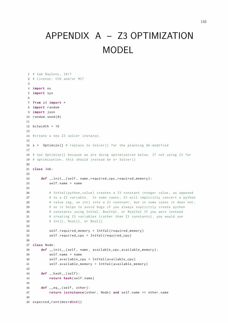
133

APPENDIX A – Z3 OPTIMIZATIONMODEL

1 # Sam Bayless , 2017

2 # License: CC0 and/or MIT

34 import os

5 import sys

67 from z3 import *

8 import random

9 import json

10 random.seed (0)

1112 bitwidth = 16

1314 #create a new Z3 solver instance.

1516 s = Optimize () # replace to Solver () for the planning OA-modified

1718 # Use Optimize () because we are doing optimization below. If not using Z3 for

19 # optimization , this should instead be s= Solver ()

2021 class Job:

2223 def __init__(self , name ,required_cpu ,required_memory):

24 self.name = name

2526 # IntVal(python_value) creates a Z3 constant integer value , as opposed

27 # to a Z3 variable. In some cases , Z3 will implicitly convert a python

28 # value (eg, an int) into a Z3 constant , but in some cases it does not ,

29 # so it helps to avoid bugs if you always explicitly create python

30 # constants using IntVal , BoolVal , or RealVal If you were instead

31 # creating Z3 variables (rather than Z3 constants), you would use

32 # Int(), Real(), or Bool()

3334 self.required_memory = IntVal(required_memory)

35 self.required_cpu = IntVal(required_cpu)

3637 class Node:

38 def __init__(self , name , available_cpu ,available_memory):

39 self.name = name

40 self.available_cpu = IntVal(available_cpu)

41 self.available_memory = IntVal(available_memory)

4243 def __hash__(self):

44 return hash(self.name)

4546 def __eq__(self , other):

47 return isinstance(other , Node) and self.name == other.name

4849 expected_runtimes=dict()

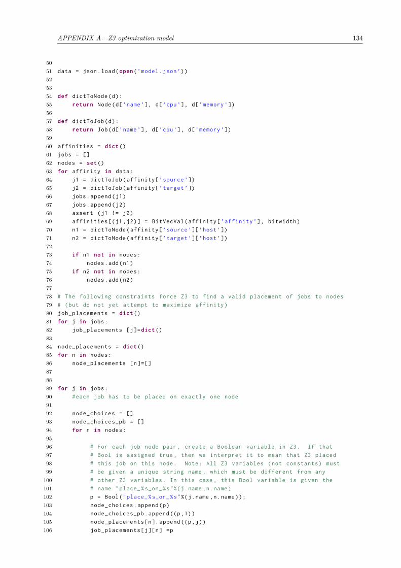
APPENDIX A. Z3 optimization model 134

5051 data = json.load(open(’model.json’))

525354 def dictToNode(d):

55 return Node(d[’name’], d[’cpu’], d[’memory ’])

5657 def dictToJob(d):

58 return Job(d[’name’], d[’cpu’], d[’memory ’])

5960 affinities = dict()

61 jobs = []

62 nodes = set()

63 for affinity in data:

64 j1 = dictToJob(affinity[’source ’])

65 j2 = dictToJob(affinity[’target ’])

66 jobs.append(j1)

67 jobs.append(j2)

68 assert (j1 != j2)

69 affinities [(j1,j2)] = BitVecVal(affinity[’affinity ’], bitwidth)

70 n1 = dictToNode(affinity[’source ’][’host’])

71 n2 = dictToNode(affinity[’target ’][’host’])

7273 if n1 not in nodes:

74 nodes.add(n1)

75 if n2 not in nodes:

76 nodes.add(n2)

7778 # The following constraints force Z3 to find a valid placement of jobs to nodes

79 # (but do not yet attempt to maximize affinity)

80 job_placements = dict()

81 for j in jobs:

82 job_placements [j]=dict()

8384 node_placements = dict()

85 for n in nodes:

86 node_placements [n]=[]

878889 for j in jobs:

90 #each job has to be placed on exactly one node

9192 node_choices = []

93 node_choices_pb = []

94 for n in nodes:

9596 # For each job node pair , create a Boolean variable in Z3. If that

97 # Bool is assigned true , then we interpret it to mean that Z3 placed

98 # this job on this node. Note: All Z3 variables (not constants) must

99 # be given a unique string name , which must be different from any

100 # other Z3 variables. In this case , this Bool variable is given the

101 # name "place_%s_on_%s"%(j.name ,n.name)

102 p = Bool("place_%s_on_%s"%(j.name ,n.name));

103 node_choices.append(p)

104 node_choices_pb.append ((p,1))

105 node_placements[n]. append ((p,j))

106 job_placements[j][n] =p

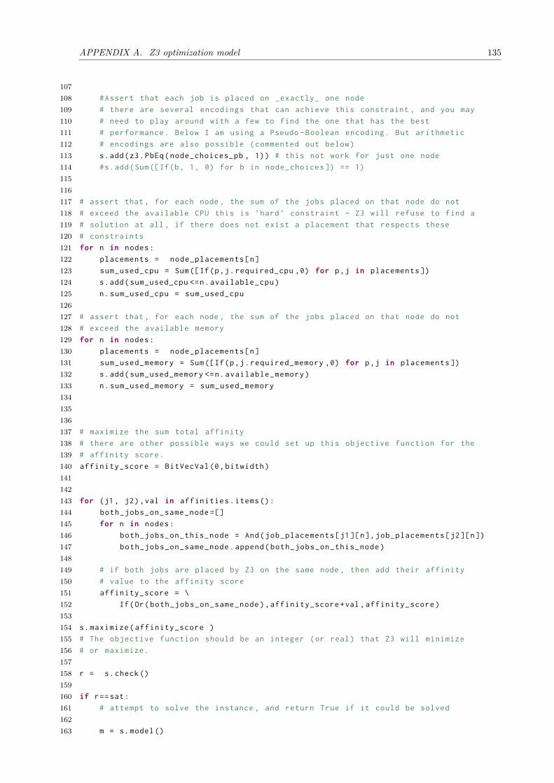
APPENDIX A. Z3 optimization model 135

107108 #Assert that each job is placed on _exactly_ one node

109 # there are several encodings that can achieve this constraint , and you may

110 # need to play around with a few to find the one that has the best

111 # performance. Below I am using a Pseudo -Boolean encoding. But arithmetic

112 # encodings are also possible (commented out below)

113 s.add(z3.PbEq(node_choices_pb , 1)) # this not work for just one node

114 #s.add(Sum([If(b, 1, 0) for b in node_choices ]) == 1)

115116117 # assert that , for each node , the sum of the jobs placed on that node do not

118 # exceed the available CPU this is ’hard’ constraint - Z3 will refuse to find a

119 # solution at all , if there does not exist a placement that respects these

120 # constraints

121 for n in nodes:

122 placements = node_placements[n]

123 sum_used_cpu = Sum([If(p,j.required_cpu ,0) for p,j in placements ])

124 s.add(sum_used_cpu <=n.available_cpu)

125 n.sum_used_cpu = sum_used_cpu

126127 # assert that , for each node , the sum of the jobs placed on that node do not

128 # exceed the available memory

129 for n in nodes:

130 placements = node_placements[n]

131 sum_used_memory = Sum([If(p,j.required_memory ,0) for p,j in placements ])

132 s.add(sum_used_memory <=n.available_memory)

133 n.sum_used_memory = sum_used_memory

134135136137 # maximize the sum total affinity

138 # there are other possible ways we could set up this objective function for the

139 # affinity score.

140 affinity_score = BitVecVal(0,bitwidth)

141142143 for (j1, j2),val in affinities.items():

144 both_jobs_on_same_node =[]

145 for n in nodes:

146 both_jobs_on_this_node = And(job_placements[j1][n],job_placements[j2][n])

147 both_jobs_on_same_node.append(both_jobs_on_this_node)

148149 # if both jobs are placed by Z3 on the same node , then add their affinity

150 # value to the affinity score

151 affinity_score = \

152 If(Or(both_jobs_on_same_node),affinity_score+val ,affinity_score)

153154 s.maximize(affinity_score )

155 # The objective function should be an integer (or real) that Z3 will minimize

156 # or maximize.

157158 r = s.check()

159160 if r==sat:

161 # attempt to solve the instance , and return True if it could be solved

162163 m = s.model()

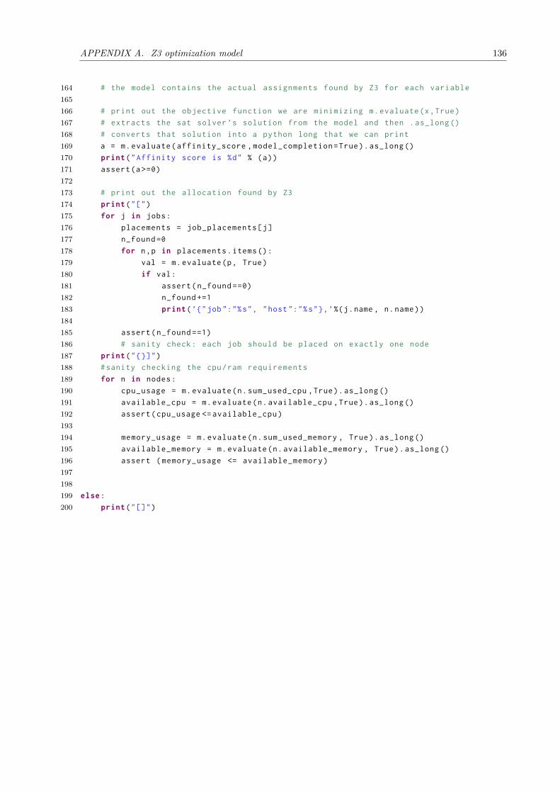
APPENDIX A. Z3 optimization model 136

164 # the model contains the actual assignments found by Z3 for each variable

165166 # print out the objective function we are minimizing m.evaluate(x,True)

167 # extracts the sat solver ’s solution from the model and then .as_long ()

168 # converts that solution into a python long that we can print

169 a = m.evaluate(affinity_score ,model_completion=True).as_long ()

170 print("Affinity score is %d" % (a))

171 assert(a>=0)

172173 # print out the allocation found by Z3

174 print("[")

175 for j in jobs:

176 placements = job_placements[j]

177 n_found =0

178 for n,p in placements.items():

179 val = m.evaluate(p, True)

180 if val:

181 assert(n_found ==0)

182 n_found +=1

183 print(’{"job ":"%s", "host ":"%s"},’%(j.name , n.name))

184185 assert(n_found ==1)

186 # sanity check: each job should be placed on exactly one node

187 print("{}]")

188 #sanity checking the cpu/ram requirements

189 for n in nodes:

190 cpu_usage = m.evaluate(n.sum_used_cpu ,True).as_long ()

191 available_cpu = m.evaluate(n.available_cpu ,True).as_long ()

192 assert(cpu_usage <= available_cpu)

193194 memory_usage = m.evaluate(n.sum_used_memory , True).as_long ()

195 available_memory = m.evaluate(n.available_memory , True).as_long ()

196 assert (memory_usage <= available_memory)

197198199 else:

200 print("[]")