1

Running head: Harmonic syntax in a blues corpus

Harmonic syntax of the twelve-bar blues form: A corpus study

Jonah Katz

316 Chitwood Hall

Dept. of World Languages, Literatures, & Linguistics

West Virginia University

Morgantown, WV 26501

Tel: +1 (617)-448-3598

Email: katzlinguist@gmail.com

2

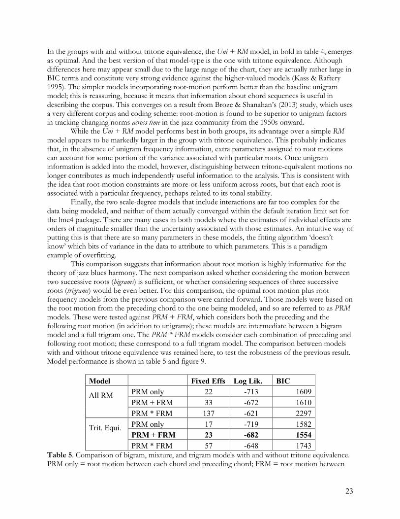
Abstract This paper describes the construction and analysis of a corpus of harmonic progressions from 12-bar blues forms included in the jazz repertoire collection The Real Book. A novel method of coding and analyzing such data is developed, using a notion of ‘possible harmonic change’ derived from the corpus and logit mixed-effects regression models describing the difference between actually occurring harmonic changes and possible but non-occurring ones in terms of various sets of theoretical constructs. Models using different sets of constructs are compared using the Bayesian Information Criterion, which assesses the accuracy and complexity of each model. The principal results are that: (1) transitional probabilities are better modeled using root-motion and chord-frequency information than they are using pairs of individual chords; (2) transitional probabilities are better described using a mixture model intermediate in complexity between a bigram and full trigram model; and (3) the difference between occurring and non-occurring chords is more efficiently modeled with a hierarchical, recursive context-free grammar than it is as a Markov chain. The results have implications for theories of harmony, composition, and cognition more generally.

3

1 Introduction This paper is an investigation of the harmonic principles active in the 12-bar blues form as used by jazz musicians. A corpus of blues forms taken from the standard repertoire collection The Real Book is used to ask questions about the musical and cognitive factors underlying the variety of harmonic structures observed in this ‘micro-genre’. Answers to these questions are sought through Bayesian comparison of logit mixed-effects regression models of the differences between occurring and possible but non-occurring chordal events. The results suggest that harmonic practice in this area is more efficiently described as deriving from root motions rather than from chord sequences and from hierarchical phrase structure rather than Markov chains. The study has three principal goals. The first one is descriptive: to validate and extend previous descriptions of the blues form (Koch 1982, Steedman 1984, Alper 2005, Love 2012). The model proposed here incorporates many of the same foundational properties as those earlier descriptions. It is, however, somewhat simpler than the previous generative model (Steedman 1984, 1996), and is explicitly justified on the basis of comparisons to finite-state models. The second goal is methodological: the study introduces a novel method for working with small musical corpora. Limiting the corpus to the harmonically rich yet relatively homogeneous micro-genre of modern jazz blues forms allows for the examination of harmonic principles somewhat more complex than the diatonic harmonies encountered in Western Art (‘classical’) music. At the same time, an empirically-derived model of the hypothesis space of possible chord changes allows more theoretical insight from a smaller corpus. The robustness of this method for basic models is tested through comparison with a more straightforward likelihood-based coding of the data, following Temperley’s (2010) work. The results suggest that the regression-based methods proposed here converge on broadly similar conclusions, but are able to ask somewhat more complex questions. I hope the method will be extended to other genres, micro- or macro-. The third goal is to address overarching issues in the structure and cognition of tonal music. These include issues in the mental representation of harmonic categories (Tymoczko 2005) and the level of formal complexity that characterizes the human faculty for harmonic composition (Tymoczko 2005, Temperley 2011, Rohrmeier 2011). The conclusions here converge on those reached by a variety of researchers studying different genres of music with rather different methods: we concur with Steedman (1984, 1996), Granroth-Wilding & Steedman (2014), Lerdahl & Jackendoff (1983), and Rohrmeier (2011) that harmonic syntax involves computations of at least context-free complexity. That said, a context-free model does best when it incorporates unigram and bigram information as well. The remainder of this section introduces and reviews previous research on harmonic syntax, the use of corpora in the study of harmonic complexity, the blues and jazz genres and songforms, and The Real Book. Section 2 reports on the creation of a blues corpus and provides an informal validation of the traditional analysis of blues form. Section 3 uses this analysis to restrict the corpus to unambiguous blues forms and compares a variety of models at different levels of analytic and computational complexity. Section 4 reviews the results of these analyses and discusses their implications for the theory of harmony more generally. 1.1 Musical harmony and syntax In most Western musical traditions, harmony refers to a system governing which sets of pitch-classes are and are not combined in compositional practice (roughly the difference between chords and non-chords) and which sequences of such chords are observed more frequently, canonically, or naturally than others. There are good introductory texts on harmony from both a music-theoretic perspective (Kostka & Payne 2013 and Aldwell & Schachter 2010 are popular university-level texts) and a cognitive-science perspective (Patel 2008, Ch. 5). Any system of constraints on the sequential

4

properties of discrete, symbolic elements invites comparisons to linguistic syntax, and this has long been the case for musical harmony (Bernstein 1976, Lerdahl & Jackendoff 1983, Steedman 1984, and Johnson-Laird 1991 are four older, influential examples). As to how similar the two systems are, there are two broad schools of thought on the subject, which can be characterized as ‘very similar’ and ‘not very similar’. Several researchers working on jazz and blues harmony have concluded that the organization of these systems is hierarchical, recursive, and/or non-regular (Steedman 1984, 1996; Johnson-Laird 1991; Granroth-Wilding & Steedman 2014). Hierarchical in this context means that entire units of music, referred to as constituents or phrases, ‘inherit’ their combinatoric properties from some harmonic event contained therein, referred to as the head of the unit. Recursive refers to structure-building processes that can be iteratively applied to their own outputs. And non-regular is a level of complexity reached by certain languages, which require phrase-structure grammars or something more complex to be generated and which can only be implemented in a machine with a memory (Chomsky 1956). These properties concern the complexity of syntactic systems, and there is broad agreement in linguistics that natural languages possess all of them (though see Pullum 2010 for a refutation of the mathematical soundness of purported proofs). So to the extent that musical genres display these types of complexity, it suggests that they are similar in a broad way to human languages. Some researchers have also suggested that the harmonic systems of Common Practice Period (CPP) ‘classical’ music are hierarchical, recursive, and/or non-regular. This work includes models oriented towards generation of harmonic structures (e.g. Rohrmeier 2011) and towards a listener’s capacity to assign structural analyses to a musical performance (Lerdahl & Jackendoff 1983, Lerdahl 2001). There is also some experimental evidence suggesting that the perception of musical tension is best modeled in a hierarchical formalism (Smith & Cuddy 2003, Lerdahl & Krumhansl 2007, though see Temperley 2011 for a dissenting interpretation of those experiments). To the extent that these authors are correct about the formal complexity of musical harmonic systems, it suggests those systems may share cognitive resources with human language. The view that musical harmony is of a complexity more or less equal to linguistic syntax, and that principles of harmony are broadly hierarchical, is far from universal. Other researchers argue that harmonic generalizations are local, finite-state and/or regular. Although there are differences in what these terms mean, they’re all associated with languages that can be generated by a finite-state machine with no memory (the regular languages proper), and in particular with the subset of such languages that produce no generalizations over non-adjacent terminal symbols (the strictly local languages). Pullum & Scholz (2009) give a brief and clear overview of these differences. Pairs of adjacent terminal elements are referred to as bigrams, sequences of more than two are referred to as trigrams, tetragrams, etc., and the general class of sequences are referred to as n-grams. Tymoczko (2005, 2010) and Temperley (2011) argue that bigram (also called first-order Markov) models do a good job of describing transitional probabilities between chords in CPP music. And indeed, many traditional textbook accounts of standard harmonic progressions, such as the ‘flow-chart’ notation used by Kostka & Payne (2013), implicitly describe finite-state automata, which give rise to regular languages. These theorists conclude that the full expressive power of a context-free grammar is far more complex than what’s needed to characterize CPP harmony, and that non-local dependencies of the kind that characterize hierarchical syntactic rules don’t really exist except for very simple ones at high levels of musical structure (Temperley 2011). If they are right, then musical harmony looks fundamentally unlike linguistic syntax. 1.2 Corpora and evaluation metrics in tonal harmony One way to adjudicate such disagreements is to look at corpora of naturally occurring sequences in some genre of music. This method is sometimes employed in linguistic syntax as well. Several

5

researchers mentioned above have put together corpora and used them to argue for one view of musical complexity or the other. The exact form of arguments from corpora varies quite a bit between different papers, and it’s worth taking a closer look at how different arguments are formed. Temperley (2009) presents a corpus consisting of 46 short excerpts from Kostka & Payne’s (1995) textbook. He argues that the most frequent bigrams in the corpus are predicted by local, finite-state theories of harmony. In his 2011 paper, he makes a similar argument, but also acknowledges that this is not a formally rigorous way of assessing the model. He points out the importance of considering overgeneration when evaluating a model: it is important to assess not only whether things that occur are predicted by a theory, but also whether things that don’t occur frequently are not predicted by the model. This will be very important in the current study. The general form of argument that involves showing some model can assign a structural description to all or nearly all of the chord sequences in some corpus is fairly common in the musical corpus literature. Steedman (1984), for instance, shows that his phrase-structure grammar of the 12-bar-blues form can generate all of the (small number of) blues forms listed in an instructional manual. At a larger scale, Tymoczko (2010) shows that his finite-state model of CPP harmony can assign a description to the vast majority of the bigrams in a corpus of 19 Mozart piano sonatas and 70 Bach chorales, better than several competing finite-state theories. In an earlier paper, Tymoczko (2005) uses a slightly different evaluation metric for another finite-state model. He shows that, when trained on the bigrams from a selection of harmonic sequences from 30 Bach chorales, a finite-state model generates a corpus of progressions that looks a lot like the original. This suggests that the bigrams must have contained a lot of important information about the corpus. Granroth-Wilding & Steedman (2014) adopt machine-learning methods from Natural Language Processing to show that a probabilistic context-free grammar parser, when trained on part of a corpus of 76 harmonic sequences from jazz lead sheets, can parse a held-out subset of the corpus more effectively than a competing finite-state (hidden Markov) model. This suggests that, while finite-state models are capable of approximating the data in the corpus, a more complex type of grammar does so more efficiently, or accurately, or both. The current study has the most in common with that of Granroth-Wilding & Steedman (GW&S). It examines jazz harmony, and applies model-selection criteria to compare finite-state and non-finite-state models of the same corpus. The current study uses a sub-genre of jazz harmony, however, the 12-bar blues form. And the studies take rather different perspectives on analyzing corpora. Most notably, while the GW&S study essentially asks ‘what is the most accurate and efficient way to parse unfamiliar chord sequences?’, the current model asks ‘what is the most plausible model for describing, a posteriori, the most important principles that went into generating this corpus?’ Of course, one would hope that the answers to these two questions would be similar, and to the extent that the current study reaches conclusions similar to those of GW&S, it can be taken as converging evidence for the nature of harmonic syntax. The differences from the other studies mentioned here are more notable, and are worth calling attention to. One of them involves the overgeneration problem mentioned by Temperley (2011): while it is certainly important that models can describe those things that occur in corpora, this can’t be taken as a convincing argument unless it can also be shown that the models fail to describe things that don’t occur in corpora. Otherwise, the best theory would simply be one where anything goes. Tymoczko (2005) implicitly gets at this point, because he examines a random sample of the output of his model and calls attention to some unusual progressions there. And given the selection criteria used by GW&S, models that assign high probabilities to infrequent events will be penalized. But the other studies mentioned above do not take account of overgeneration.

6

A second issue involves parsimony. It is a mathematical certainty that any finite corpus can be approximated by either finite-state or context-free models, given a sufficient number of parameters (Tymoczko 2010; Rohrmeier, Fu, & Dienes 2012). So showing that one type of model can approximate a finite corpus is not particularly informative. The other main criterion we have at our disposal for evaluating competing models is simplicity: how efficiently models represent the information in the corpus. The only way to make use of this criterion is to trade off the fit of the model (how well it describes the data) against its complexity. Tymoczko (2010) assumes that, because context-free grammars (CFGs) are inherently more complex than finite-state ones, showing that a finite-state model can approximate a corpus means that a CFG should be dispreferred. But this depends on the specific models: while a CFG is more complex than a finite-state model in the limited sense of requiring a memory to implement, it could still be true that a CFG with few parameters encodes information as well as a finite-state model with many more parameters. In this case, there is a sense in which the CFG would be less complex (Rohrmeier, Fu, and Dienes 2012 make a similar point in the context of linguistic syntax).

Intuitively, we seek a formal model that balances the simultaneous values of ‘correctness’ (goodness-of-fit) and simplicity (lack of complexity). The best way to assess fit and complexity is to use an explicit model-comparison criterion to select between competing models. This study uses the Bayesian Information Criterion (BIC) to compare regression models, which can be seen as an implementation of the Minimum Description Length approach (see Mavromatis 2009 and Temperley 2010 for applications to music corpora). In this approach, model fit and complexity are both measured in terms of the length of the description required to specify both data (relevant to fit) and model (relevant to complexity). Given a certain type of prior distribution for parameter estimates, the MDL approach to regression models is equivalent to the current approach (Stine 2004). There are a variety of MDL methods, and no general consensus on what types of priors are best; the current procedure has the advantage of being easy to implement with a standard software package for mixed-effects regression modeling.

Another strain of corpus modeling in music uses methods based on cross-entropy (e.g. Conklin & Witten 1995; Pearce & Wiggins 2004; Temperley 2010). This work tends to be concerned with melody and rhythm more than harmony, but the basic principles are the same. Cross-entropy is, in this context, a way of measuring how close the distribution of events predicted by a model is to the distribution of events in an actual corpus. The regression-based method used here minimizes a cost function that is closely related to the cross-entropy of the model and the corpus, so it has much in common with the cross-entropy approach. The data here, however, are coded rather differently than in other studies of this kind.

A typical approach to corpora using cross-entropy codes the surface properties of one or more melodic voices: pitch, duration, etc. N-gram models are then fit to the coded properties based on empirical probabilities in the corpus, and cross-entropy is assessed with regard to (all or part of) the corpus. Conceptually, this can be thought of as a model of composition, in which each parameter of the musical surface (pitch, duration, etc.) has a characteristic probability distribution and the composer draws events from that distribution. The compositional model used in the current study, and hence the coding of the data, is rather different.

The coding used here is based on chord changes and derived from Lerdahl & Jackendoff’s (1983) theory of reductions. The overarching idea is that the blues form is a basic structure (referred to here as a skeleton) containing an essential sequence of chords. Additions to this basic structure occur when the composer chooses to elaborate on or expand one of the events in the structure, according to some finite-state or hierarchical principle of expansion. In between any two events contained in the skeleton, therefore, a set of choices to expand or not expand will produce a variety of chord changes. In this study, each expansion is treated as a binary choice: in between any two chords, there

7

is a (possibly null) set of expansions that occur, as well as a variety of expansions that could have occurred in that location but did not. The use of ‘possible expansions’ that did not occur makes these data somewhat different from the cross-entropy-based studies cited above. The selection of possible but non-occurring expansions is derived from the corpus itself and described in section 3.1.

While this approach to coding the data is novel and somewhat idiosyncratic, it has certain desirable properties. For one, it means that the data can be described with logistic regression models, which are easy to fit, have standard evaluation metrics, and allow modeling of random effects such as composer and song. A second useful property is that it allows relatively straightforward coding of parameters associated with non-finite-state models of harmony: a CFG predicts that some expansions are allowed and others are not. Assessing how well these distinctions match the occurring and non-occurring expansions in the corpus is straightforward. Finally, restricting the ‘attention’ of harmonic models to a limited set of possible chord changes makes them easier to fit: if every possible outcome (chord) in every metrical position were considered, the vast majority of the data would consist of 0s, and probabilistic models (regression or otherwise) do not perform well under those circumstances. While there are a variety of smoothing and other techniques developed to deal with low-probability events in corpora, the current approach avoids the problem altogether.

One concern is that, because the data and modeling procedures used here are so different from standard cross-entropy approaches, any results may be due to idiosyncratic properties of these novel methods. While this possibility can’t be entirely ruled out, section 3.5 shows that, for the simpler finite-state models evaluated here, the results largely converge with those of a more standard cross-entropy-based approach using only occurring features.

1.3 Blues, jazz, and jazz blues The term ‘blues’ is used in at least three different ways: blues genre, blues inflection, and blues form. This can be confusing for those familiar with the term but not familiar with the music, so I give a very brief introduction to each of them here. For more detailed historical background on the blues, see Alper (2005), Palmer (1981), and Lomax (1993).

The blues genre is, like most genres, not an absolute category but a useful label for a collection of styles that frequently mix with non-blues traditions. It is a type of folk or popular music that arose amongst black musicians in the American South sometime prior to the turn of the 20th century. It may be related to earlier African forms, but the historical record is rather sparse. One well-known early 20th-century blues genre is the ‘country blues’ (which is sometimes subdivided into regional variations), generally involving solo acoustic guitar and vocals. Robert Johnson, Son House, and Blind Lemon Jefferson are good exemplars of this style, which often incorporated elements of ragtime and non-blues folk genres. As black workers migrated north following World War II, the blues went with them. Urban blues of this period often make use of electric guitars and full bands: Muddy Waters and Howlin’ Wolf in Chicago are perhaps the two best-known performers of this period, though Memphis also had a thriving blues community. The electric blues of the 1940s and 1950s had a heavy influence on (or, one could say, became) early rock n’ roll.

Blues ‘inflection’ is my term for some of the stylistic devices typical of the blues genre. This includes a wide variety of melodic maneuvers, often based on minor pentatonic scales with conventionalized passing tones, pitch-bending, grace-note ornamentations, and relative lack of sensitivity to the harmonic background of a piece of music. This is the sense in which one might describe a melodic gesture as a ‘blues lick’ or a vocal performance as ‘bluesy’.

Finally, blues forms are a set of strophic song-forms that arose in the blues genre. By far the most common is a form with 12 groupings (‘bars’) of 4 tactus-level beats, generally with triple subdivisions beneath that tactus level. The particular harmonic and metrical properties of this form are referred to as the 12-bar blues. At its most basic level, the form involves a I-IV-I-V-I

8

progression aligned with particular metrical positions in the 12-bar structure. This is the type of blues form I’m concerned with in this paper. It is a form that the reader is almost certainly familiar with, even if not consciously. The 12-bar blues form is ubiquitous in rock and other popular genres: some famous examples include ‘Hound Dog’, ‘Johnny B. Goode’, ‘In the Mood’, ‘Folsom Prison Blues’, ‘Corrina, Corrina’, ‘The Ballad of John and Yoko’, and ‘Should I Stay or Should I Go’.

These three meanings of ‘blues’ are related to some extent, but not coextensive. The blues genre almost always uses blues inflection, but blues inflection is also common in many other genres of music. Many of the songs performed in the blues genre are 12-bar blues forms, but these forms are also used in many other genres, as the list above was meant to suggest. The corpus developed in this study consists of blues forms, but not in the blues genre. Instead, I examine the form as adopted by post-war jazz musicians.

The earliest period of blues history was characterized by frequent overlap and interchange with early jazz music, and blues forms have been an important part of the jazz repertoire for much of the last century. Performers such as Ma Rainey and Bessie Smith in the 1920s drew freely from both traditions, illustrating the often ‘fuzzy’ boundary between them and suggesting that jazz and blues genres may be better viewed as lying on a continuum of styles. In the 1940s, jazz musicians began to elaborate upon the blues form in ways that are highly interesting from the perspective of harmonic syntax. These post-war jazz blues forms will be the focus of the corpus constructed here. We refer to the broad style of jazz beginning in this period (often called bebop) and dominant until the 1960s as ‘modern jazz’, to distinguish it from earlier ‘classic jazz’ and the eclectic mix of styles emerging in the 1960s and 1970s which are referred to as ‘contemporary jazz’.

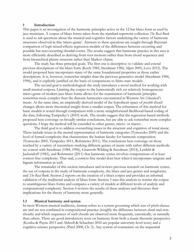
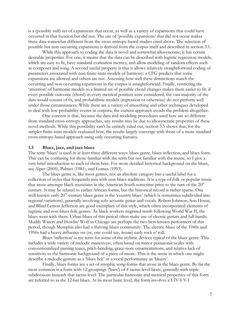
There are several reasons why the modern jazz blues is useful for this type of study. One is that it clearly involves some type of active, implicit harmonic generalization on the part of performers. The rules and tendencies investigated here are understood well enough that even inexperienced jazz musicians frequently improvise blues forms, both by themselves and in coordination with other musicians in a group. These improvisations do not always have identical chords, but pattern rather like variations on a theme. As such, it follows that musicians do not only memorize chord sequences, but acquire implicit cognitive principles that dictate what types of chord sequences are consistent with the blues form. Host & Ashley (2006) use experimental evidence to argue that such principles are active in blues-form perception as well. Some of these principles are discussed in the next section. 1.4 The blues form The 12-bar blues form can be traced from a relatively simple harmonic structure in early styles to ever-more-complicated variations on that form extending to the present. Here I briefly discuss the development of the modern jazz blues form. All of the generalizations I propose here agree with basic descriptions in Koch (1982), Steedman (1984), Alper (2005), and/or Love (2012). The canonical form from early blues genre recordings, such as Robert Johnson’s, is shown in figure 1.

Figure 1. An early blues-genre form, with distinctive elements boxed. Metrical ‘x’ marks correspond to full measures, generally in 12/8 time.

What is the blues?

A very basic blues form, from early blues genre performances: 1 2 3 4 5 6 7 8 9 10 11 12 1 repeat x x x x x x x x x x x x x x x x x x x x x x x x … I (IV I) IV I V IV I I The blues form contains a few harmonic sequences that are not canonical in CPP or jazz harmony: •!the IV chord in measure 5 has an implied dominant 7 quality

o!includes the b3 scale degree o!chord is very infrequent in CPP and (non-blues) jazz

•!the V-IV-I cadence in measures 9-11 is virtually unheard of in non-blues forms in these genres

•!a 12-bar repeating form in general is unusual for jazz

9

For all illustrations of musical form in this paper, I use the Lerdahl & Jackendoff (1983) metrical grid notation familiar to linguists and cognitive musicologists, with roman-numeral notation for harmonies. Parentheses indicate optional elements. Each metrical position in this figure represents an entire measure. Note that while I’ve used traditional Western chord-symbols to represent harmony here, it is not obvious that performers like Johnson are actually using the harmonic categories of, for instance, CPP music in any straightforward way. The third is sometimes omitted in these chords, the melodies performed over them do not always clearly imply a major or minor quality, and it may be more useful to think of the harmonic structure as a relatively invariant complex of bass voices against which modal melodic material unfolds.

Several features of the form in figure 1 are not consistent with jazz or CPP norms. The IV chord in measure 5 generally has an implied �7 quality, because melodies played or sung over it often include the �3 scale degree. The IV�7 chord is very infrequent in CPP, and infrequent in jazz except as a blues inflection (henceforth, I refer to these flat-seven chords as plain ‘7’, in accordance with jazz norms). The V-IV-I cadence in this blues form is virtually unheard of in non-blues jazz forms. And the non-binary 12-bar form itself, organized into three 4-bar groups, is highly unusual in jazz, which tends to have a preponderance of 8-, 16-, and 32-bar forms.

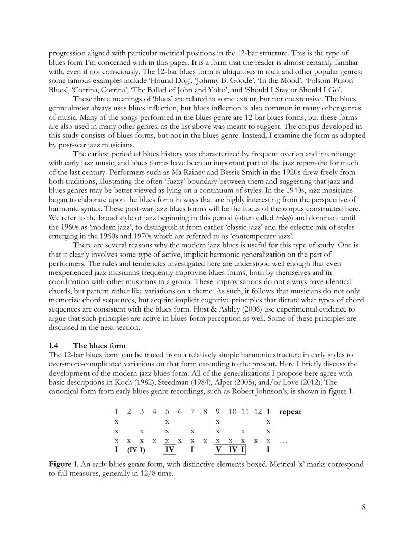
Pre-war jazz blues performances generally featured more typical jazz chord voicings rather than the modal guitar accompaniment mentioned above. However, they retained several other distinctive blues features, making these performances relatively easy to distinguish from ‘general’ jazz repertoire. A typical form from this period is shown in figure 2, corresponding roughly to Billie Holiday’s 1936 recording of ‘Billie’s Blues’.

Figure 2. A typical pre-war jazz blues form, based on ‘Billie’s Blues’ by Billie Holiday. One of the distinctive blues elements retained here is the dominant quality of the I7 and IV7 chords, which are not otherwise idiomatic in jazz repertoire. The 12-bar metrical form itself has been retained, which is otherwise unusual in jazz. The V-IV-I cadence, however, has been replaced here by the ii7-V7-I more typical of jazz. This is not a universal feature of jazz blues performances; sometimes the V-IV-I is retained.

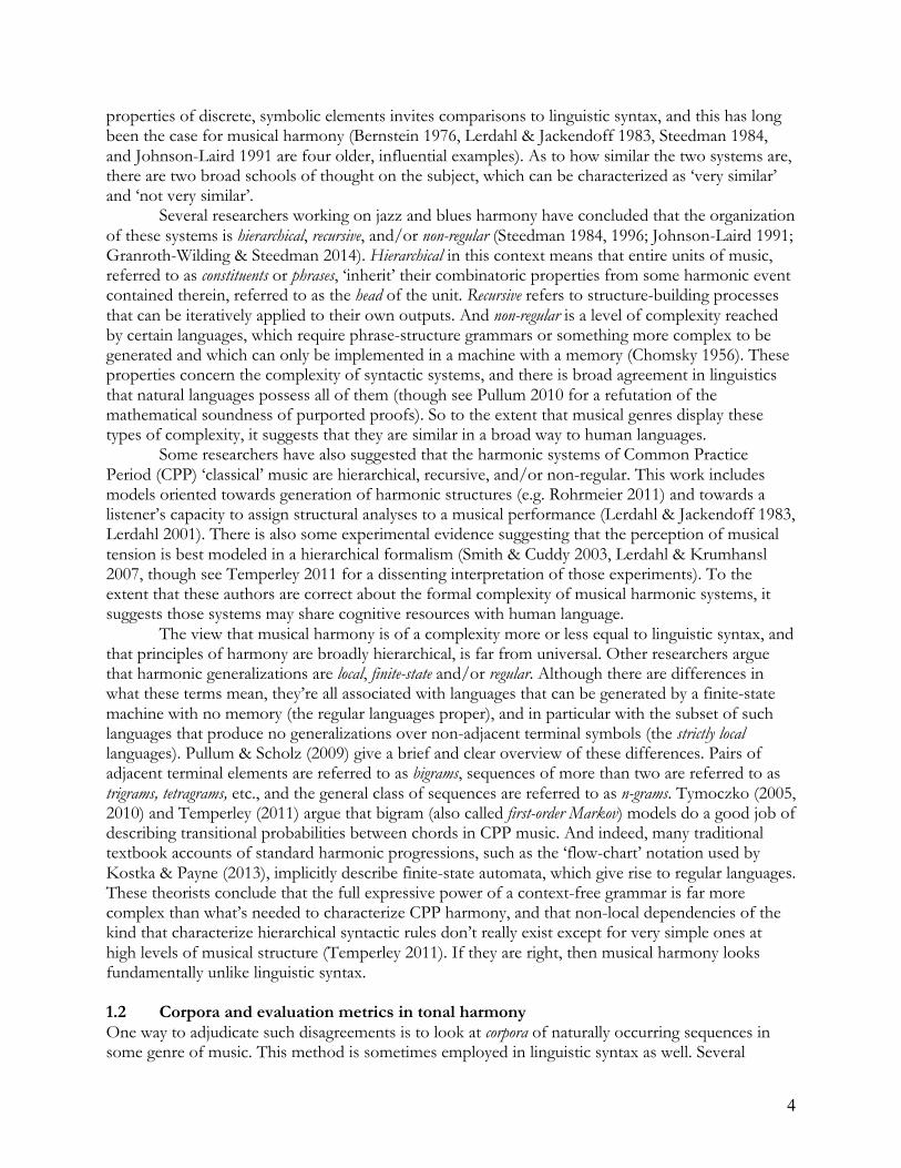
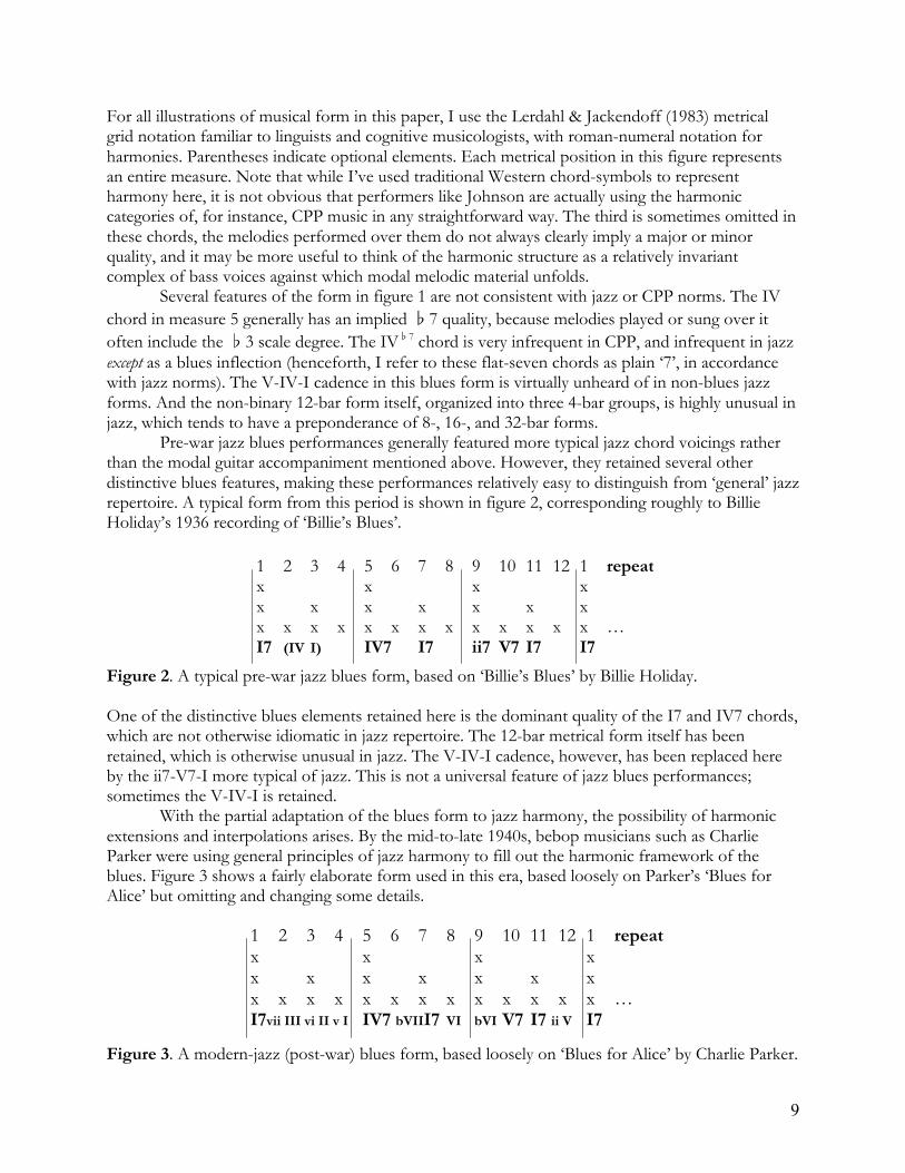
With the partial adaptation of the blues form to jazz harmony, the possibility of harmonic extensions and interpolations arises. By the mid-to-late 1940s, bebop musicians such as Charlie Parker were using general principles of jazz harmony to fill out the harmonic framework of the blues. Figure 3 shows a fairly elaborate form used in this era, based loosely on Parker’s ‘Blues for Alice’ but omitting and changing some details.

Figure 3. A modern-jazz (post-war) blues form, based loosely on ‘Blues for Alice’ by Charlie Parker.

What is the blues?

1 2 3 4 5 6 7 8 9 10 11 12 1 repeat x x x x x x x x x x x x x x x x x x x x x x x x … I7 (IV I) IV7 I7 ii7 V7 I7 I7 Sometime in the range 1920-1945, jazz musicians began to extend and change this form: •!generally keeping the distinctive dominant quality of the IV chord

in m. 5 •!often adding an unusual dominant quality to tonic (I) chords •!but often eliminating the unidiomatic V-IV-I cadence in favor of

a more conventional V or ii-V cadence

What is the blues?

1 2 3 4 5 6 7 8 9 10 11 12 1 repeat x x x x x x x x x x x x x x x x x x x x x x x x … I7vii III vi II v I IV7 bVIII7 VI bVI V7 I7 ii V I7 By the late 1940s, jazz musicians are creating far more complex versions of the blues progression: •!keeping its distinctive blues structural elements

o!which are not generally a property of jazz harmony •!but interpolating between them using principles of jazz harmony

10

The form in figure 3 retains the major structural elements of the 12-bar blues form: the opening tonic, the crucial IV in measure 5, and the cadence in measures 9-11. But elaborations drawn from the bebop harmonic lexicon ‘fill in’ this blues skeleton. Most notably, the form is full of chromatic chords or modulations, which tend to follow general root-motion principles by downward 5th or half-step, but otherwise don’t appear to be much constrained by the overall tonality of the piece.

The example is a fairly good illustration of principles of modern jazz harmony (see Johnson-Laird 1991, Broze & Shanahan 2013, and Granroth-Wilding & Steedman 2014 for detailed expositions). The principles of this genre are clearly related to CPP harmony: pieces tend to begin and end on tonic, the local tonic tends to be approached by perfect cadence, and root-motion tends to proceed by downard 5th. But many of the details differ.

While CPP music often prepares a cadential V using a IV chord, modern jazz very rarely does so, primarily using ii instead. In contrast to CPP harmony, chromatic chords and modulations in modern jazz are frequent, dense, and often target distant keys without pivot chords or other preparation. All chords are taken to implicitly allow for upper voices such as the 7th, 9th, and 13th to be present in their performance; the exact ways in which these ‘extensions’ are included in chord voicings is part of a complex improvisational process known as ‘comping’. The principle of tritone substitution, mostly absent from CPP harmony, allows for the function of any chord except for the tonic to be fulfilled by a chord whose root is a tritone away. This means that root-motion by descending semitone can substitute for root motion by descending fifth, and makes �II7-I a fairly standard cadence. Finally, while the major, minor, and diminshed quality of chords is largely dictated by the local key in CPP harmony, these constraints are much looser in modern jazz. There are definite tendencies pertaining to chord quality, but they are always subject to exceptions. Taken together, these differences mean that the notion of ‘key’, with all of its harmonic entailments, is just somewhat looser in modern jazz than in CPP music (see Shanahan & Broze 2012 for discussion). Nonetheless, most pieces do clearly have a global tonic (the atonal and ‘free’ jazz that began to emerge in the 1960s differs in this respect).

Because of its relative clear overarching form coupled with complexity in terms of chromaticism, substitution, and chord-density, the jazz blues is an excellent object for syntactic study. That is why I have chosen it for this project. One difficulty, however, is deciding what counts as ‘repertoire’ in this genre. In the next section, I describe the source from which harmonic generalizations are drawn in this paper. 1.5 The Real Book The Real Book is an illegal collection of ‘lead sheets’ for copyrighted jazz pieces that circulated by mimeograph and under-the-counter sales from sometime in the 1970s until the advent of digital file-sharing.1 It is correspondingly unclear who created the collection. Musicians such as Pat Metheny and Steve Swallow associated with the Berklee School of Music appear to have been involved (Kernfeld 2006). There is little scholarly literature on the book, although Young & Matheson (2000) briefly discuss it and it is frequently used as a data source in computational studies of jazz (e.g. Anglade & Dixon 2008, Eigenfeldt & Pasquier 2010). Shanahan & Broze (2012) discuss the wider ‘fake-book culture’ from which The Real Book emerged. The Real Book contains some contemporary material from the 1970s, but its main use is as a compendium of standard jazz repertoire from the 1930s to 1960s, often based on show tunes from

1 A reviewer notes that a legal version of The Real Book is now sold by the Hal Leonard company. The website suggests that it may differ from the original in both repertoire and specific details of transcription.

11

earlier eras. It corresponds in some sense to a ‘canon’ that all jazz musicians should be familiar with, and so I treat it here as being broadly representative of modern jazz. One felicitous property of The Real Book is that it represents pieces as lead sheets, an abstract, symbolic form that can be easily translated into corpus data. The lead sheet contains, in the general case, a notated melody line and harmonic structure abbreviated to the level of chord symbols. For instance, during a stretch of music where the underlying harmony is A minor 7, a piano player may produce several distinct note collections in different metrical positions in a performance, but The Real Book will notate the entire temporal interval as ‘A-7’.

This compression creates the possibility for disagreements over which chord symbol fits a performance best, and there is a general feeling in the jazz community that The Real Book contains ‘errors’. But the vast majority of its contents are reasonably sound. There is a legal collection called The New Real Book, published in 3 volumes by the Sher Music Company, which has some overlap with the original bootleg version. While this version has not been as influential in terms of repertoire, it does often have higher-quality transcriptions than the original. Wherever one of the songs in the corpus is contained in both versions, I’ve used the symbols from The New Real Book. 2 A blues corpus Both traditional (Koch 1982, Alper 2005, Love 2012) and generative (Steedman 1984) descriptions of the blues form agree on certain basic structural elements: the overall form is a kind of metrical/harmonic skeleton, with a I chord at the beginning, a IV chord on measure 5, a return to I on measure 7, and a cadence in measures 9-11. Further elaborations may be ‘built off of’ the elements in this skeleton. While these observations seem completely trivial to an experienced jazz musician, it is worth trying to validate them on some independent basis. That is what I attempt to do in this section. 2.1 Selection criteria The first question that arises is how to choose an empirical domain against which to test these hypotheses without being tautological. The clearest way to identify a blues form is to hear it and intuit that it’s a blues form. But if those intuitions are based on precisely the harmonic criteria just discussed, then showing that a corpus selected in such a manner obeys those criteria is circular. For a preliminary corpus, I instead took advantage of the unusual 12-bar metrical pattern associated with the form. Because this pattern is otherwise unusual in jazz, picking all of the 12- (or 24-) measure forms in The Real Book will result in a corpus that mainly contains blues forms. This forms a basis for drawing harmonic generalizations about the blues from a ‘canon’ selected on a non-harmonic basis. Once the basic structural elements of the blues have been confirmed, the corpus can be winnowed down to exclude non-blues forms and test specific theories of blues structure. There are 39 pieces by 25 composers in The Real Book containing a repeating form of either 12 or 24 notated measures, and these comprise the preliminary corpus. The full list is given in Appendix A. By my intuitions, 4 of these are pretty clearly not blues forms, and 5 or so could be argued about one way or the other. The remaining 30 or so are clearly blues forms. All 39 songs were converted to a representation of chord roots relative to the tonic associated with particular metrical positions in the 12-bar form. 24 metrical subdivisions, each corresponding to two beats in a typical time signature, were sufficient to accommodate all of the chord sequences in these pieces. These charts are also included in Appendix A.

There were not enough data in the corpus to separate chords by quality (e.g. 7, Maj7, -7, ø7), so they were coded only in terms of their roots. This undoubtedly loses some information, although in the general case chord quality is fairly unconstrained in this form. Note that most of the hard and fast generalizations that hold about chord quality are long-distance in nature. For instance, the

12

distinction between minor- and major-key blues is not coded here. The main differences between the two modes are that the iv chord is generally minor in a minor-key blues, major in a major-key one; and that the minor-key form almost always contains a �VI7 before the cadential dominant, while the major-key form can contain either this chord or a ii of some kind. These global considerations would not be captured by any of the models considered here, even if chord quality were coded. These generalizations would require a theory of key constraints; we do not attempt to formulate such a theory here. A few chord notations from The Real Book that seemed obviously wrong to me were changed to reflect recordings of the pieces in question. For instance, ‘Swedish Pastry’ by Barney Kessel is notated with a tonic return in measure 8, but scale degree 3 in the bass is clearly audible in the Bill Evans recording cited as the source for the Real Book transcription. One additional consideration was how to deal with fully-diminished 7th chords. They generally ‘stand in’ for dominant 7th chords in this genre, with the root of the diminshed chord being the 3rd of an implicit dominant 7th (Schoenberg 1911 and Piston 1941 suggest something similar can occur in CPP harmony, but this is far from universally accepted). Because this affects the root-motion possibilities of such sequences, fully diminished chords were coded as having an implicit root a major 3rd below the notated root.

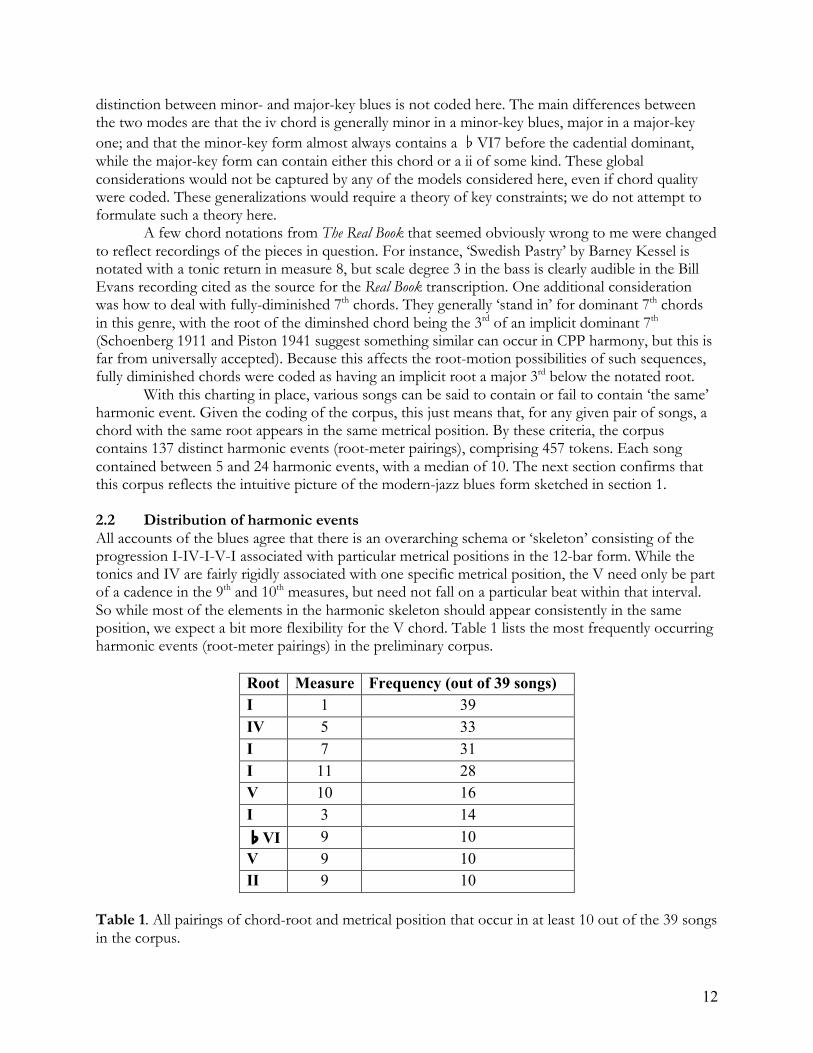
With this charting in place, various songs can be said to contain or fail to contain ‘the same’ harmonic event. Given the coding of the corpus, this just means that, for any given pair of songs, a chord with the same root appears in the same metrical position. By these criteria, the corpus contains 137 distinct harmonic events (root-meter pairings), comprising 457 tokens. Each song contained between 5 and 24 harmonic events, with a median of 10. The next section confirms that this corpus reflects the intuitive picture of the modern-jazz blues form sketched in section 1. 2.2 Distribution of harmonic events All accounts of the blues agree that there is an overarching schema or ‘skeleton’ consisting of the progression I-IV-I-V-I associated with particular metrical positions in the 12-bar form. While the tonics and IV are fairly rigidly associated with one specific metrical position, the V need only be part of a cadence in the 9th and 10th measures, but need not fall on a particular beat within that interval. So while most of the elements in the harmonic skeleton should appear consistently in the same position, we expect a bit more flexibility for the V chord. Table 1 lists the most frequently occurring harmonic events (root-meter pairings) in the preliminary corpus.

Root Measure Frequency (out of 39 songs) I 1 39 IV 5 33 I 7 31 I 11 28 V 10 16 I 3 14 �VI 9 10 V 9 10 II 9 10

Table 1. All pairings of chord-root and metrical position that occur in at least 10 out of the 39 songs in the corpus.

13

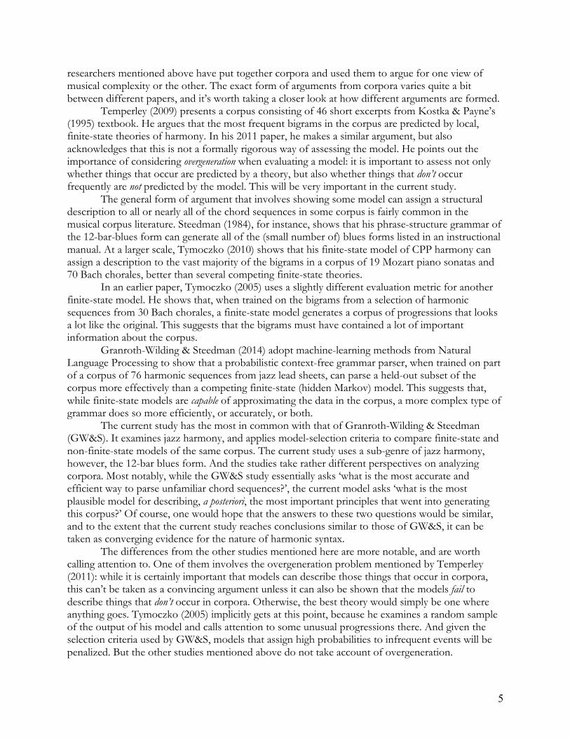
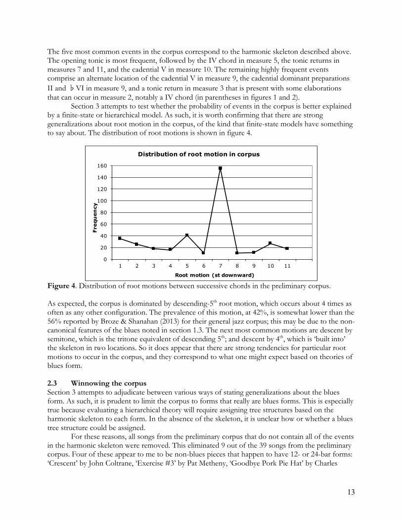
The five most common events in the corpus correspond to the harmonic skeleton described above. The opening tonic is most frequent, followed by the IV chord in measure 5, the tonic returns in measures 7 and 11, and the cadential V in measure 10. The remaining highly frequent events comprise an alternate location of the cadential V in measure 9, the cadential dominant preparations II and �VI in measure 9, and a tonic return in measure 3 that is present with some elaborations that can occur in measure 2, notably a IV chord (in parentheses in figures 1 and 2). Section 3 attempts to test whether the probability of events in the corpus is better explained by a finite-state or hierarchical model. As such, it is worth confirming that there are strong generalizations about root motion in the corpus, of the kind that finite-state models have something to say about. The distribution of root motions is shown in figure 4.

Figure 4. Distribution of root motions between successive chords in the preliminary corpus. As expected, the corpus is dominated by descending-5th root motion, which occurs about 4 times as often as any other configuration. The prevalence of this motion, at 42%, is somewhat lower than the 56% reported by Broze & Shanahan (2013) for their general jazz corpus; this may be due to the non-canonical features of the blues noted in section 1.3. The next most common motions are descent by semitone, which is the tritone equivalent of descending 5th; and descent by 4th, which is ‘built into’ the skeleton in two locations. So it does appear that there are strong tendencies for particular root motions to occur in the corpus, and they correspond to what one might expect based on theories of blues form. 2.3 Winnowing the corpus Section 3 attempts to adjudicate between various ways of stating generalizations about the blues form. As such, it is prudent to limit the corpus to forms that really are blues forms. This is especially true because evaluating a hierarchical theory will require assigning tree structures based on the harmonic skeleton to each form. In the absence of the skeleton, it is unclear how or whether a blues tree structure could be assigned. For these reasons, all songs from the preliminary corpus that do not contain all of the events in the harmonic skeleton were removed. This eliminated 9 out of the 39 songs from the preliminary corpus. Four of these appear to me to be non-blues pieces that happen to have 12- or 24-bar forms: ‘Crescent’ by John Coltrane, ‘Exercise #3’ by Pat Metheny, ‘Goodbye Pork Pie Hat’ by Charles

0

20

40

60

80

100

120

140

160

1 2 3 4 5 6 7 8 9 10 11

Freq

uen

cy

Root motion (st downward)

Distribution of root motion in corpus

14

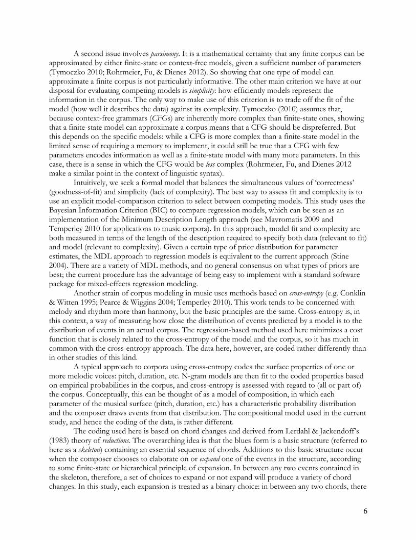
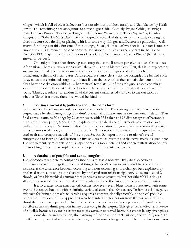
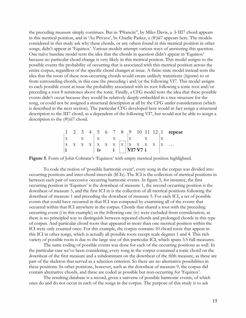
Mingus (which is full of blues inflections but not obviously a blues form), and ‘Semblance’ by Keith Jarrett. The remaining 5 are ambiguous to some degree: ‘Blue Comedy’ by Joe Gibbs, ‘Henniger Flats’ by Gary Burton, ‘Las Vegas Tango’ by Gil Evans, ‘Nostalgia in Times Square’ by Charles Mingus, and ‘Solar’ by Miles Davis. By my judgment, several of these are pretty clearly evoking the blues structure but altering or playing with it in some way. Mingus and Burton are particularly well-known for doing just this. For one of these songs, ‘Solar’, the issue of whether it is a blues is unclear enough that it is a frequent topic of conversation amongst musicians and appears in the title of Pachet’s (1997) paper ‘Computer Analysis of Jazz Chord Sequences: Is Solar a Blues?’ (he takes the answer to be ‘yes’). One might object that throwing out songs that some listeners perceive as blues forms loses information. There are two reasons why I think this is not a big problem. First, this is an exploratory analysis and it makes sense to examine the properties of unambiguous blues forms before formulating a theory of fuzzy cases. And second, it’s fairly clear what the principles are behind such fuzzy cases: the eliminated songs seem blues-like to the extent that they contain elements of the blues harmonic skeleton within a 12-bar metrical template: all of the ambiguous cases contain at least 3 of the 5 skeletal events. While this is surely not the only criterion that makes a song-form sound ‘bluesy’, it suffices to explain all of the current examples. My answer to the question of whether ‘Solar’ is a blues, therefore, would be ‘kind of’. 3 Testing structural hypotheses about the blues form In this section I compare several theories of the blues form. The starting point is the narrower corpus made by eliminating songs that don’t contain all of the events in the harmonic skeleton. That final corpus contains 30 songs by 21 composers, with 333 tokens of 98 distinct types of harmonic event (root-meter pairing). Section 3.1 explains how the database of harmonic information was coded from this corpus. Section 3.2 describes the phrase-structure grammar that was used to assign tree structures to the songs in the corpus. Section 3.3 describes the statistical techniques that were used to fit and compare models of the corpus. Section 3.4 reports on the results of several comparisons of interest. And section 3.5 investigates the robustness of the novel methods used here. The supplementary materials for this paper contain a more detailed and concrete illustration of how the modeling procedure is implemented for a pair of representative events. 3.1 A database of possible and actual songforms The approach taken here to comparing models is to assess how well they do at describing differences between things that occur and things that don’t occur in particular blues pieces. For instance, is the difference between occurring and non-occurring chord changes best explained by preferred metrical positions for changes, by preferred root relationships between sequences of 2 chords, or by a hierarchical grammar that generates some structures but not others? This design allows for assessment of both the descriptive adequacy and the parsimony of potential theories. It also creates some practical difficulties, however: every blues form is associated with some events that occur, but also with an infinite variety of events that don’t occur. To harness this negative evidence for human or machine learning requires a computationally tractable notion of ‘possible event that didn’t occur’. The approach taken here infers such a notion from the corpus itself: any chord that occurs in a particular rhythmic position somewhere in the corpus is considered to be possible at that rhythmic position in any other song in the corpus. This gives us, in effect, a universe of possible harmonic events to compare to the actually observed harmonic events in any given piece. Consider, as an illustration, the harmony of John Coltrane’s ‘Equinox’, shown in figure 5. In the 8th measure, marked with a rectangle here, no harmonic change occurs. The tonic harmony from

15

the preceding measure simply continues. But in ‘Pfrancin’’, by Miles Davis, a �III7 chord appears in this metrical position, and in ‘Au Privave’, by Charlie Parker, a (#)iii7 appears here. The models considered in this study ask why these chords, or any others found in this metrical position in other songs, didn’t appear in ‘Equinox’. Various models attempt various ways of answering this question. One naïve baseline model tests the idea that the chords in question didn’t appear in ‘Equinox’ because no particular chord change is very likely in this metrical positon. This model assigns to the possible events the probability of occurring that is associated with this metrical position across the entire corpus, regardless of the specific chord changes at issue. A finite-state model instead tests the idea that the roots of these non-occurring chords would create unlikely transitions (bigrams) to or from surrounding chords, in this case the preceding i and/or the following VI7. This model assigns to each possible event at issue the probability associated with its root following a tonic root and/or preceding a root 8 semitones above the tonic. Finally, a CFG model tests the idea that these possible events didn’t occur because they would be relatively deeply embedded in a tree structure for the song, or could not be assigned a structural description at all by the CFG under consideration (which is described in the next section). The particular CFG developed here would in fact assign a structural description to the III7 chord, as a dependent of the following VI7, but would not be able to assign a description to the (#)iii7 chord.

Figure 5. Form of John Coltrane’s ‘Equinox’ with empty metrical position highlighted. To code the notion of ‘possible harmonic event’, every song in the corpus was divided into occurring positions and inter-chord intervals (ICIs). The ICI is the collection of metrical positions in between each pair of successive occurring harmonic events. In figure 5, for instance, the first occurring position in ‘Equinox’ is the downbeat of measure 1, the second occurring position is the downbeat of measure 5, and the first ICI in is the collection of all metrical positions following the downbeat of measure 1 and preceding the downbeat of measure 5. For each ICI, a set of possible events that could have occurred in that ICI was computed by examining all of the events that occurred within that ICI anywhere in the corpus. Chords that shared a root with the preceding occurring event (i in this example) or the following one (iv) were excluded from consideration, as there is no principled way to distinguish between repeated chords and prolonged chords in this type of corpus. And particular chord roots that appeared in more than one metrical position within the ICI were only counted once. For this example, the corpus contains 10 chord roots that appear in this ICI in other songs, which is actually all possible roots except scale degrees 1 and 4. This rich variety of possible roots is due to the large size of this particular ICI, which spans 3.5 full measures. The same coding of possible events was done for each of the occurring positions as well. In the particular case we’ve been considering, every song in the corpus contained a tonic chord on the downbeat of the first measure and a subdominant on the downbeat of the fifth measure, as these are part of the skeleton that served as a selection criterion. So there are no alternative possibilities in these positions. In other positions, however, such as the downbeat of measure 9, the corpus did contain alternative chords, and these are coded as possible but non-occurring for ‘Equinox’. The resulting database is a record, given a universe of possible harmonic events, of which ones do and do not occur in each of the songs in the corpus. The purpose of this study is to ask

Corpus materials

For instance: Equinox (John Coltrane) 1 2 3 4 5 6 7 8 9 10 11 12 1 repeat x x x x x x x x x x x x x x x x x x x x … i iv i VI7 V7 i In bar 8 here, no harmonic change happens •!but in Pfrancin’ (Miles Davis), a III7 chord appears here •!and in Au Privave (Charlie Parker), a (#)iii chord appears here

The model will then ask: why didn’t these chords appear in this piece? Possible kinds of answers: •!this is an unlikely rhythmic position for a chord change •!the roots of these chords would create unlikely bigrams with

surrounding ones •!these chords can’t be assigned a structural description by a CFG

16

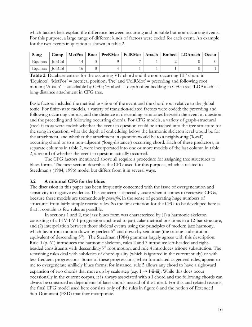
which factors best explain the difference between occurring and possible but non-occurring events. For this purpose, a large range of different kinds of factors were coded for each event. An example for the two events in question is shown in table 2.

Song Comp MetPos Root PreRMot FolRMot Attach Embed LDAttach Occur Equinox JohCol 14 3 9 7 1 2 0 0 Equinox JohCol 16 8 4 1 1 1 0 1

Table 2. Database entries for the occurring VI7 chord and the non-occurring III7 chord in ‘Equinox’. ‘MetPos’ = metrical position; ‘Pre’ and ‘FolRMot’ = preceding and following root motion; ‘Attach’ = attachable by CFG; ‘Embed’ = depth of embedding in CFG tree; ‘LDAttach’ = long-distance attachment in CFG tree. Basic factors included the metrical position of the event and the chord root relative to the global tonic. For finite-state models, a variety of transition-related factors were coded: the preceding and following occurring chords, and the distance in descending semitones between the event in question and the preceding and following occurring chords. For CFG models, a variety of graph-structural (tree) factors were coded: whether the event in question could be attached into the tree structure for the song in question, what the depth of embedding below the harmonic skeleton level would be for the attachment, and whether the attachment in question would be to a neighboring (‘local’) occurring chord or to a non-adjacent (‘long-distance’) occurring chord. Each of these predictors, in separate columns in table 2, were incorporated into one or more models of the last column in table 2, a record of whether the event in question actually occurred. The CFG factors mentioned above all require a procedure for assigning tree structures to blues forms. The next section describes the CFG used for this purpose, which is related to Steedman’s (1984, 1996) model but differs from it in several ways. 3.2 A minimal CFG for the blues The discussion in this paper has been frequently concerned with the issue of overgeneration and sensitivity to negative evidence. This concern is especially acute when it comes to recursive CFGs, because these models are tremendously powerful, in the sense of generating huge numbers of structures from fairly simple rewrite rules. So the first criterion for the CFG to be developed here is that it contain as few rules as possible. In sections 1 and 2, the jazz blues form was characterized by (1) a harmonic skeleton consisting of a I-IV-I-V-I progression anchored to particular metrical positions in a 12-bar structure, and (2) interpolation between those skeletal events using the principles of modern jazz harmony, which favor root motion down by perfect 5th and down by semitone (the tritone-stubstitution equivalent of descending 5th). The Steedman (1984) grammar largely agrees with this description: Rule 0 (p. 61) introduces the harmonic skeleton, rules 2 and 3 introduce left-headed and right-headed constituents with descending-5th root motion, and rule 4 introduces tritone substitution. The remaining rules deal with subtleties of chord quality (which is ignored in the current study) or with less frequent progressions. Some of these progressions, when formulated as general rules, appear to me to overgenerate unlikely blues forms; for instance, rule 5 allows any chord to have a rightward expansion of two chords that move up by scale step (e.g. I → I-ii-iii). While this does occur occasionally in the current corpus, it is always associated with a I chord and the following chords can always be construed as dependents of later chords instead of the I itself. For this and related reasons, the final CFG model used here consists only of the rules in figure 6 and the notion of Extended Sub-Dominant (ESD) that they incorporate.

17

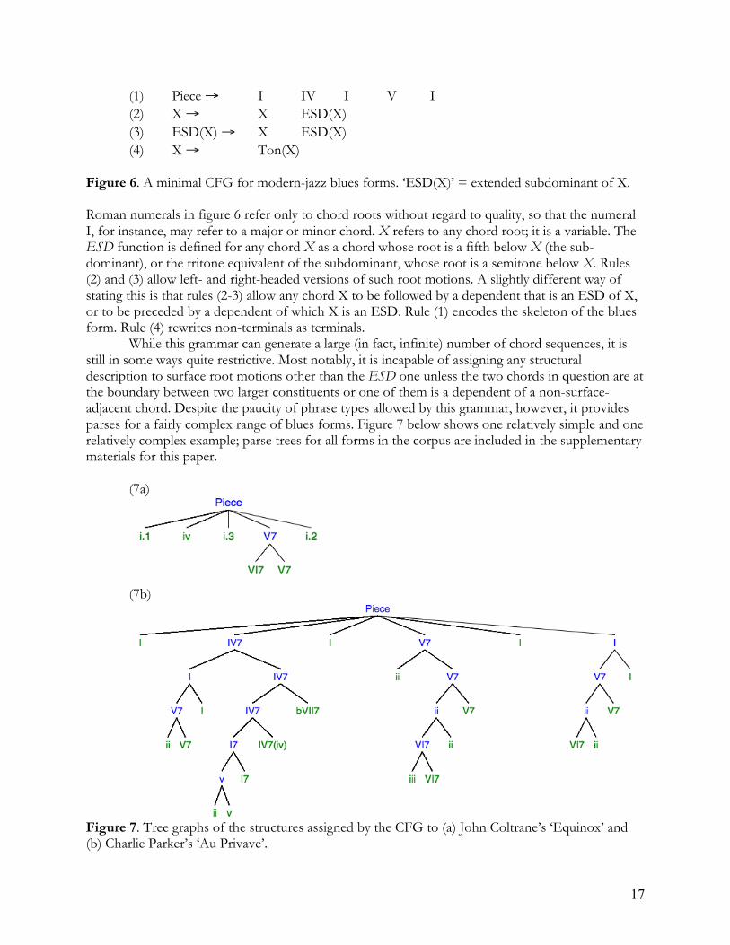
(1) Piece → I IV I V I (2) X → X ESD(X) (3) ESD(X) → X ESD(X) (4) X → Ton(X)

Figure 6. A minimal CFG for modern-jazz blues forms. ‘ESD(X)’ = extended subdominant of X. Roman numerals in figure 6 refer only to chord roots without regard to quality, so that the numeral I, for instance, may refer to a major or minor chord. X refers to any chord root; it is a variable. The ESD function is defined for any chord X as a chord whose root is a fifth below X (the sub-dominant), or the tritone equivalent of the subdominant, whose root is a semitone below X. Rules (2) and (3) allow left- and right-headed versions of such root motions. A slightly different way of stating this is that rules (2-3) allow any chord X to be followed by a dependent that is an ESD of X, or to be preceded by a dependent of which X is an ESD. Rule (1) encodes the skeleton of the blues form. Rule (4) rewrites non-terminals as terminals. While this grammar can generate a large (in fact, infinite) number of chord sequences, it is still in some ways quite restrictive. Most notably, it is incapable of assigning any structural description to surface root motions other than the ESD one unless the two chords in question are at the boundary between two larger constituents or one of them is a dependent of a non-surface-adjacent chord. Despite the paucity of phrase types allowed by this grammar, however, it provides parses for a fairly complex range of blues forms. Figure 7 below shows one relatively simple and one relatively complex example; parse trees for all forms in the corpus are included in the supplementary materials for this paper.

(7a)

(7b)

Figure 7. Tree graphs of the structures assigned by the CFG to (a) John Coltrane’s ‘Equinox’ and (b) Charlie Parker’s ‘Au Privave’.

18

In the simple example of ‘Equinox’ (7a), every event in the piece is part of the skeleton assigned by rule (1) except for the pre-cadential VI7 chord. This chord is licensed as a dependent of the cadential V by rule (3), because V is an ESD of (�)VI. In the more complex example of ‘Au Privave’ (7b), the skeleton is present on the horizontal immediately below ‘Piece’, and several of these skeleton events have their own dependents. The vast majority of all the expansions in this tree are licensed by the right-headed rule (3); the only exception is the IV → IV �VII in mm. 5-6; the �VII is an ESD of the IV chord, and is licensed as a dependent by left-headed rule (2). Several aspects of these structures are worthy of comment. The ‘Piece’ level is represented as a flat structure here, with all skeletal harmonic events being immediate dependents of that level. This corresponds to a stipulation within the theory advanced here that the blues form cannot be derived from more basic principles of jazz harmony: it is a memorized structure that derives from partially arbitrary and accidental history and cultural conventions. That said, while the blues form is not entirely explicable in terms of jazz harmony, it is also clearly not entirely arbitrary. Many of the chords and transitions in the blues skeleton are possible in jazz, and the cadence is a standard ending for almost every piece in modern jazz. I would speculate that the blues form became a staple in jazz repertoire because it is distinct enough from standard jazz practice to enhance variety in the genre, but not so distinct from genre norms that it would be impossible to assimilate it into the tradition. The corpus contains some examples of chords that cannot be assigned a structural description by the CFG introduced here. For instance, the A section of ‘African Flower’ by Duke Ellington contains a �iii7 chord in between the measure-5 subdominant and the tonic return in measure 7. Such chords were coded as ‘unattachable’; the most straightforward prediction of the CFG model is that they should not be licensed; the probabilistic implementation in terms of regression models used here would then predict they should be infrequent. Finally, note that this grammar (and all others considered here) does not explain the alignment of harmonic material with absolute metrical positions (e.g., ‘IV chord appears in on the downbeat of measure 5’). I take constraints on metrical alignment to be a part of the memorized schema for the blues and not something to be explained by the harmonic system. With all songs in the corpus assigned a tree structure, it is possible to code the structural factors listed in section 3.1. For instance, the VI7 in ‘Equinox’ above would be coded as attachable, locally dependent, and 1 level of embedding down from the skeletal tier. The second tonic chord in ‘Au Privave’ would be coded as attachable, non-locally dependent, and 1 level of embedding down from the skeletal tier. A variety of non-occuring but possible events, according to the criteria in section 3.1, were coded for the position that they would occupy if they had occurred. The full database of possible events in the corpus is included in the supplementary materials, along with tree-structure representations of each song. The next step is to compare various models’ characterization of the difference between occurring and possible but non-occurring events. 3.3 Modeling and model-comparison Given that the outcome of interest here is a binary one, occurrence or non-occurrence, I use logistic regression to examine the effect of various factors on that outcome. In logistic regression, the log odds (or logit) of some outcome occurring is modeled in terms of a set of independent variables. The current models contain two kinds of variables. Fixed effects are variables that are systematically varied across a predetermined number of levels; in the current study, these include the structural and root-motion factors discussed in section 3.1. Random effects are variables whose levels are randomly sampled from some larger population of interest. Here, these would include ‘song’ and ‘composer’; the corpus doesn’t include every modern-jazz blues form, nor every composer of such forms. Instead, the corpus includes a hopefully representative sample determined by the authors of The Real

19

Book. The best way to incorporate fixed and random effects into a single model is with mixed-effects regression; Jaeger (2008) and Quené & van den Bergh (2008) give excellent and accessible overviews of mixed-effects logistic regression models. The models here were implemented with the lme4 package (v. 1.1-10, Bates et al. 2015) in the statistical platform R. All structural, chord-root, and metrical factors were coded as fixed effects, while composer and song were coded as random effects. This structure allows us to test whether the fixed effects of primary interest here robustly affect the probability of chords occurring across different levels of random variables. Because the song and composer random effects did not end up explaining significant amounts of variance in the models where both were included, and including more random variables makes model-fitting more computationally difficult and time-consuming, only the effects of song were retained in the final models reported here. Once various models are fitted to the data in the corpus, they need to be compared. Given that the blues corpus created here is finite in size, it will be possible to approximate that corpus using either a finite-state model or a CFG one. This is a mathematical necessity: in the most extreme case, we could simply give either a finite-state or CFG model one parameter for every single occurring and non-occurring event in the corpus and they would fit the data perfectly. This would be true even if the finite corpus were full of recursive center-embedding structures (it is not), as long as they’re finite. A more relevant question is whether the regularities in the corpus are more accurately or efficiently expressed by some models than by others. And answering that question requires a way of comparing models of different types. The best criterion for comparing different kinds of models of the same data is a fairly complex and interesting question in and of itself. The choice made here is to use the Bayesian (or Schwarz) Information Criterion (BIC). Kadane & Lazar (2004) and Vrieze (2012) give overviews of the BIC and compare it to other criteria. All literature on the BIC contains a fair bit of mathematics that is impenetrable to non-experts (myself included), but the overarching concepts involved in the model-selection process are relatively clear. As noted in section 1.2, the BIC can be viewed as an application of Minimum-Description-Length methodology to model selection, where a particular kind of prior over parameters is assumed. The BIC is inversely proportional to the Bayesian posterior probability of some model, that is, the probability that the model is correct given the data that have been observed. Selecting a model using the BIC involves looking for the model with the lowest BIC value, thus maximizing the posterior probability amongst the models being considered. The posterior probability, in Bayes’ equation, is proportional to the probability of the observed data given the model (the likelihood) and the prior probability of that model. In cases like the current study, where it is not entirely clear what the prior probability of any model is, the BIC in effect uses the number of free parameters in the model in place of priors: more complex models are less probable a priori, all else being equal. Note that the ‘observed’ data here includes occurring chords but also non-occurring possible chords as described in section 3.1. This selection process will reward models for goodness of fit (expressed in terms of likelihood) and penalize models for including many parameters. This is precisely what is required for an exercise like the current one, where it is unclear not only which parameters are the most relevant to blues harmony, but also how many parameters are optimal for describing the system. The BIC differs from the related Akaike Information Criterion (AIC) in how sharply it penalizes overfitting. In general, the BIC has a much larger penalty for extra parameters than the AIC and tends to favor smaller models. This is because both criteria incorporate estimation uncertainty, while only the BIC incorporates parameter uncertainty. In conceptual terms, one can say that the AIC may be better for predicting future outcomes, because it allows for relatively subtle parameters to enter the model, but the BIC is better for describing the most meaningful factors that

20

went into generating the observed outcomes. Because the purpose of this study is to discover which parameters are most useful for describing the blues form, the BIC was used here. All of the model comparisons reported with BIC values here, however, were also run with the less stringent AIC for the sake of completeness. Qualitative patterns of results were very similar, in particular the comparisons between families of models, although a few of the family-internal results came out differently with the AIC. A concrete example of exactly how the modeling process works for a pair of representative events is included in the supplementary materials for this paper. 3.4 Evaluating models of the blues This section reports on the construction of models of the harmonic database described in sections 2 and 3, and Bayesian model selection from amongst those alternatives. Section 3.4.1 establishes a ‘baseline’ model with no information on harmonic sequences, to ensure that more sophisticated harmonic models are actually doing something useful. Section 3.4.2 selects an optimal finite-state model, adjudicating between different notions of harmonic categories and different orders of Markov model. Section 3.4.3 selects an optimal CFG-based model, adjudicating between various structural criteria (depth of embedding, locality of dependencies, etc.) for describing the difference between more and less likely events. And section 3.4.4 reports on a more conservative test of the hypothesis that CFGs represent the corpus more efficiently than finite-state models. More detailed summaries of the optimal models from each section are included in the supplementary materials. 3.4.1 Rhythmic and chordal baselines Before even talking about principles of harmonic combinatorics, it makes sense to investigate more basic kinds of information that affect the probability of a chord occurring: the root of the chord (relative to tonic) and its metrical position. Some chords are more frequent than others in this genre, due to a combination of appearing in the obligatory harmonic skeleton of the blues form, harmonic stability, and/or proximity to the tonic. On all three counts, we would expect tonic chords to be most frequent, followed by subdominant and dominant chords, and that in and of itself constitutes information. It is also a fact that some metrical positions are obligatorily filled by a harmonic change in the form, while others are not, and therefore events that take place in stronger metrical positions are more likely. Models based on either or both of these two parameters do not include any direct information about motion from one chord to another, yet they capture non-trivial information about the corpus. In this section, an optimal model incorporating these factors is selected. Based on descriptions of the blues form, it would be quite surprising if one of these models turned out to be the best. If models in subsequent sections, which include information on harmonic motion, do not improve on this ‘baseline’ model, we can conclude that either something is wrong with the corpus (e.g. it doesn’t contain enough data to form meaningful generalizations) or that harmonic generalizations about the blues form are ‘noisy’ enough that it is best to state them in terms of a list of chords that are more likely to occur and metrical positions that are more likely to host a chord change. On the other hand, if the baseline model is improved by adding information about harmonic sequences, we can conclude that the corpus contains sufficient data to produce meaningful generalizations about combinatorics and that relationships between chords are a crucial part of the theory of blues form. Four rhythmic and chordal candidate models were fitted. ‘Rt only’ uses only the chord-root of an event to predict probability of occurrence; this corresponds to the hypothesis that some chords are more frequent than others, and there are no other generalizations to be had. ‘Pos only’ used only metrical position to predict probability of occurrence; this corresponds to the hypothesis

21

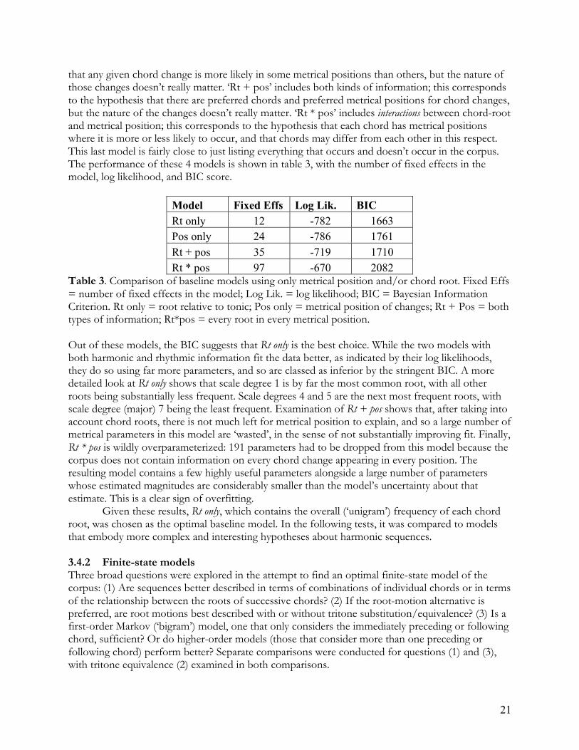
that any given chord change is more likely in some metrical positions than others, but the nature of those changes doesn’t really matter. ‘Rt + pos’ includes both kinds of information; this corresponds to the hypothesis that there are preferred chords and preferred metrical positions for chord changes, but the nature of the changes doesn’t really matter. ‘Rt * pos’ includes interactions between chord-root and metrical position; this corresponds to the hypothesis that each chord has metrical positions where it is more or less likely to occur, and that chords may differ from each other in this respect. This last model is fairly close to just listing everything that occurs and doesn’t occur in the corpus. The performance of these 4 models is shown in table 3, with the number of fixed effects in the model, log likelihood, and BIC score.

Model Fixed Effs Log Lik. BIC Rt only 12 -782 1663 Pos only 24 -786 1761 Rt + pos 35 -719 1710 Rt * pos 97 -670 2082

Table 3. Comparison of baseline models using only metrical position and/or chord root. Fixed Effs = number of fixed effects in the model; Log Lik. = log likelihood; BIC = Bayesian Information Criterion. Rt only = root relative to tonic; Pos only = metrical position of changes; Rt + Pos = both types of information; Rt*pos = every root in every metrical position. Out of these models, the BIC suggests that Rt only is the best choice. While the two models with both harmonic and rhythmic information fit the data better, as indicated by their log likelihoods, they do so using far more parameters, and so are classed as inferior by the stringent BIC. A more detailed look at Rt only shows that scale degree 1 is by far the most common root, with all other roots being substantially less frequent. Scale degrees 4 and 5 are the next most frequent roots, with scale degree (major) 7 being the least frequent. Examination of Rt + pos shows that, after taking into account chord roots, there is not much left for metrical position to explain, and so a large number of metrical parameters in this model are ‘wasted’, in the sense of not substantially improving fit. Finally, Rt * pos is wildly overparameterized: 191 parameters had to be dropped from this model because the corpus does not contain information on every chord change appearing in every position. The resulting model contains a few highly useful parameters alongside a large number of parameters whose estimated magnitudes are considerably smaller than the model’s uncertainty about that estimate. This is a clear sign of overfitting. Given these results, Rt only, which contains the overall (‘unigram’) frequency of each chord root, was chosen as the optimal baseline model. In the following tests, it was compared to models that embody more complex and interesting hypotheses about harmonic sequences. 3.4.2 Finite-state models Three broad questions were explored in the attempt to find an optimal finite-state model of the corpus: (1) Are sequences better described in terms of combinations of individual chords or in terms of the relationship between the roots of successive chords? (2) If the root-motion alternative is preferred, are root motions best described with or without tritone substitution/equivalence? (3) Is a first-order Markov (‘bigram’) model, one that only considers the immediately preceding or following chord, sufficient? Or do higher-order models (those that consider more than one preceding or following chord) perform better? Separate comparisons were conducted for questions (1) and (3), with tritone equivalence (2) examined in both comparisons.

22

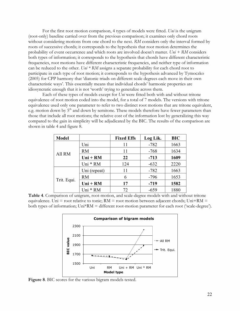
For the first root motion comparison, 4 types of models were fitted. Uni is the unigram (root-only) baseline carried over from the previous comparison; it examines only chord roots without considering motions from one chord to the next. RM considers only the interval formed by roots of successive chords; it corresponds to the hypothesis that root motion determines the probability of event occurrence and which roots are involved doesn’t matter. Uni + RM considers both types of information; it corresponds to the hypothesis that chords have different characteristic frequencies, root motions have different characteristic frequencies, and neither type of information can be reduced to the other. Uni * RM assigns a separate probability for each chord root to participate in each type of root motion; it corresponds to the hypothesis advanced by Tymoczko (2005) for CPP harmony that ‘diatonic triads on different scale degrees each move in their own characteristic ways’. This essentially means that individual chords’ harmonic properties are idiosyncratic enough that it is not ‘worth’ trying to generalize across them. Each of these types of models except for Uni were fitted both with and without tritone equivalence of root motion coded into the model, for a total of 7 models. The versions with tritone equivalence used only one parameter to refer to two distinct root motions that are tritone equivalent, e.g. motion down by 5th and down by semitone. These models therefore have fewer parameters than those that include all root motions; the relative cost of the information lost by generalizing this way compared to the gain in simplicity will be adjudicated by the BIC. The results of the comparison are shown in table 4 and figure 8.

Model Fixed Effs Log Lik. BIC

All RM

Uni 11 -782 1663 RM 11 -768 1634 Uni + RM 22 -713 1609 Uni * RM 124 -632 2220

Trit. Equi.

Uni (repeat) 11 -782 1663 RM 6 -796 1653 Uni + RM 17 -719 1582 Uni * RM 72 -659 1880

Table 4. Comparison of unigram, root-motion, and scale-degree models with and without tritone equivalence. Uni = root relative to tonic; RM = root motion between adjacent chords; Uni+RM = both types of information; Uni*RM = different root-motion parameter for each root (‘scale-degree’).

Figure 8. BIC scores for the various bigram models tested.

1500

1700

1900

2100

2300

Uni RM Uni + RM Uni * RM

BIC

va

lue

Model type

Comparison of bigram models

All RM

Trit. Equi.

23

In the groups with and without tritone equivalence, the Uni + RM model, in bold in table 4, emerges as optimal. And the best version of that model-type is the one with tritone equivalence. Although differences here may appear small due to the large range of the chart, they are actually rather large in BIC terms and constitute very strong evidence against the higher-valued models (Kass & Raftery 1995). The simpler models incorporating root-motion perform better than the baseline unigram model; this is reassuring, because it means that information about chord sequences is useful in describing the corpus. This converges on a result from Broze & Shanahan’s (2013) study, which uses a very different corpus and coding scheme: root-motion is found to be superior to unigram factors in tracking changing norms across time in the jazz community from the 1950s onward. While the Uni + RM model performs best in both groups, its advantage over a simple RM model appears to be markedly larger in the group with tritone equivalence. This probably indicates that, in the absence of unigram frequency information, extra parameters assigned to root motions can account for some portion of the variance associated with particular roots. Once unigram information is added into the model, however, distinguishing between tritone-equivalent motions no longer contributes as much independently useful information to the analysis. This is consistent with the idea that root-motion constraints are more-or-less uniform across roots, but that each root is associated with a particular frequency, perhaps related to its tonal stability. Finally, the two scale-degree models that include interactions are far too complex for the data being modeled, and neither of them actually converged within the default iteration limit set for the lme4 package. There are many cases in both models where the estimates of individual effects are orders of magnitude smaller than the uncertainty associated with those estimates. An intuitive way of putting this is that there are so many parameters in these models, the fitting algorithm ‘doesn’t know’ which bits of variance in the data to attribute to which parameters. This is a paradigm example of overfitting. This comparison suggests that information about root motion is highly informative for the theory of jazz blues harmony. The next comparison asked whether considering the motion between two successive roots (bigrams) is sufficient, or whether considering sequences of three successive roots (trigrams) would be even better. For this comparison, the optimal root motion plus root frequency models from the previous comparison were carried forward. Those models were based on the root motion from the preceding chord to the one being modeled, and so are referred to as PRM models. These were tested against PRM + FRM, which considers both the preceding and the following root motion (in addition to unigrams); these models are intermediate between a bigram model and a full trigram one. The PRM * FRM models consider each combination of preceding and following root motion; these correspond to a full trigram model. The comparison between models with and without tritone equivalence was retained here, to test the robustness of the previous result. Model performance is shown in table 5 and figure 9.

Model Fixed Effs Log Lik. BIC

All RM

PRM only 22 -713 1609 PRM + FRM 33 -672 1610 PRM * FRM 137 -621 2297

Trit. Equi.

PRM only 17 -719 1582 PRM + FRM 23 -682 1554 PRM * FRM 57 -648 1743

Table 5. Comparison of bigram, mixture, and trigram models with and without tritone equivalence. PRM only = root motion between each chord and preceding chord; FRM = root motion between

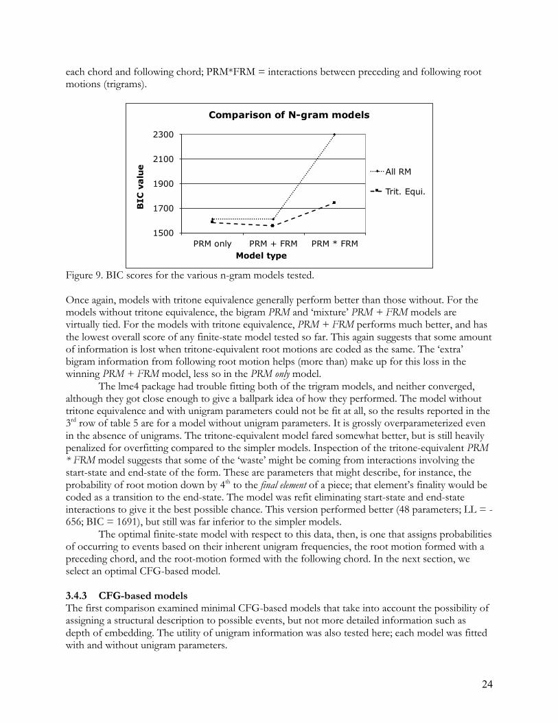
24

each chord and following chord; PRM*FRM = interactions between preceding and following root motions (trigrams).

Figure 9. BIC scores for the various n-gram models tested. Once again, models with tritone equivalence generally perform better than those without. For the models without tritone equivalence, the bigram PRM and ‘mixture’ PRM + FRM models are virtually tied. For the models with tritone equivalence, PRM + FRM performs much better, and has the lowest overall score of any finite-state model tested so far. This again suggests that some amount of information is lost when tritone-equivalent root motions are coded as the same. The ‘extra’ bigram information from following root motion helps (more than) make up for this loss in the winning PRM + FRM model, less so in the PRM only model. The lme4 package had trouble fitting both of the trigram models, and neither converged, although they got close enough to give a ballpark idea of how they performed. The model without tritone equivalence and with unigram parameters could not be fit at all, so the results reported in the 3rd row of table 5 are for a model without unigram parameters. It is grossly overparameterized even in the absence of unigrams. The tritone-equivalent model fared somewhat better, but is still heavily penalized for overfitting compared to the simpler models. Inspection of the tritone-equivalent PRM * FRM model suggests that some of the ‘waste’ might be coming from interactions involving the start-state and end-state of the form. These are parameters that might describe, for instance, the probability of root motion down by 4th to the final element of a piece; that element’s finality would be coded as a transition to the end-state. The model was refit eliminating start-state and end-state interactions to give it the best possible chance. This version performed better (48 parameters; LL = -656; BIC = 1691), but still was far inferior to the simpler models. The optimal finite-state model with respect to this data, then, is one that assigns probabilities of occurring to events based on their inherent unigram frequencies, the root motion formed with a preceding chord, and the root-motion formed with the following chord. In the next section, we select an optimal CFG-based model. 3.4.3 CFG-based models The first comparison examined minimal CFG-based models that take into account the possibility of assigning a structural description to possible events, but not more detailed information such as depth of embedding. The utility of unigram information was also tested here; each model was fitted with and without unigram parameters.

1500

1700

1900

2100

2300

PRM only PRM + FRM PRM * FRM

BIC

va

lue

Model type

Comparison of N-gram models

All RM

Trit. Equi.

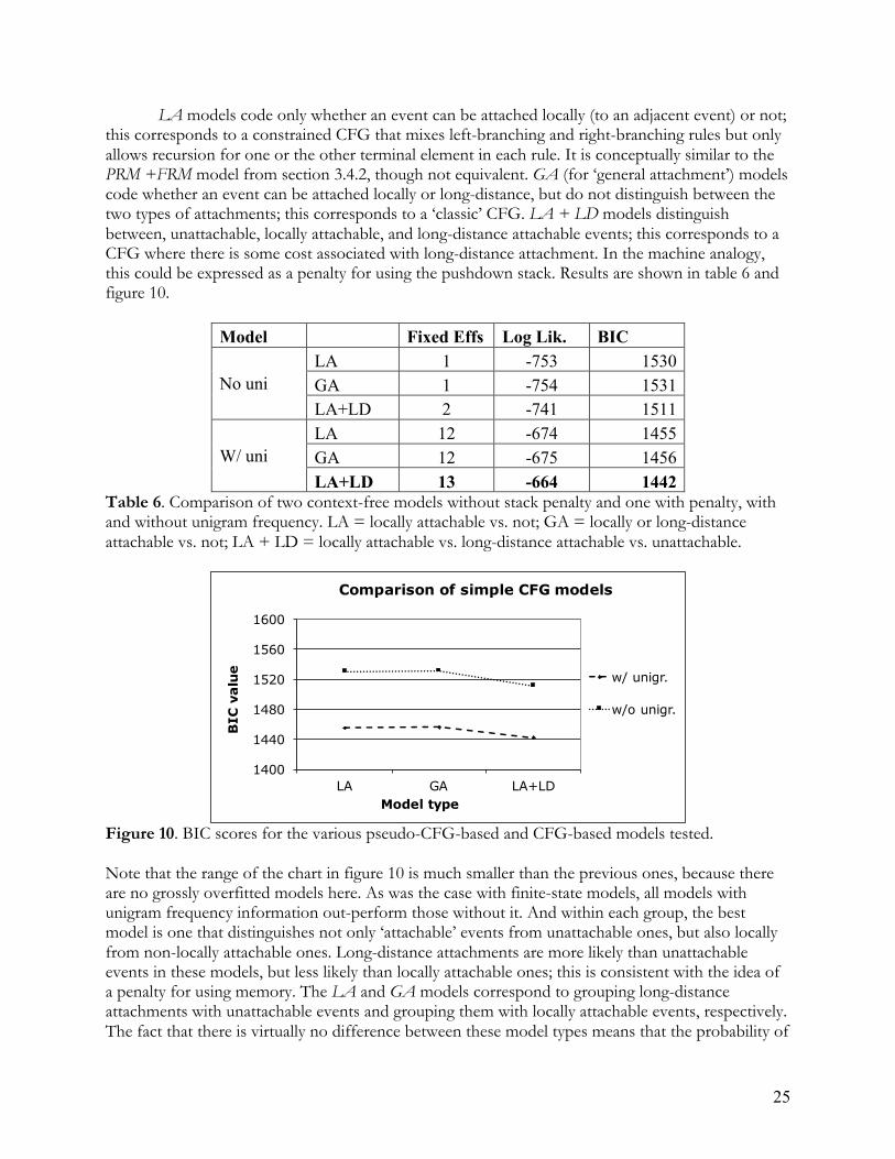
25

LA models code only whether an event can be attached locally (to an adjacent event) or not; this corresponds to a constrained CFG that mixes left-branching and right-branching rules but only allows recursion for one or the other terminal element in each rule. It is conceptually similar to the PRM +FRM model from section 3.4.2, though not equivalent. GA (for ‘general attachment’) models code whether an event can be attached locally or long-distance, but do not distinguish between the two types of attachments; this corresponds to a ‘classic’ CFG. LA + LD models distinguish between, unattachable, locally attachable, and long-distance attachable events; this corresponds to a CFG where there is some cost associated with long-distance attachment. In the machine analogy, this could be expressed as a penalty for using the pushdown stack. Results are shown in table 6 and figure 10.

Model Fixed Effs Log Lik. BIC

No uni LA 1 -753 1530 GA 1 -754 1531 LA+LD 2 -741 1511

W/ uni LA 12 -674 1455 GA 12 -675 1456 LA+LD 13 -664 1442

Table 6. Comparison of two context-free models without stack penalty and one with penalty, with and without unigram frequency. LA = locally attachable vs. not; GA = locally or long-distance attachable vs. not; LA + LD = locally attachable vs. long-distance attachable vs. unattachable.

Figure 10. BIC scores for the various pseudo-CFG-based and CFG-based models tested. Note that the range of the chart in figure 10 is much smaller than the previous ones, because there are no grossly overfitted models here. As was the case with finite-state models, all models with unigram frequency information out-perform those without it. And within each group, the best model is one that distinguishes not only ‘attachable’ events from unattachable ones, but also locally from non-locally attachable ones. Long-distance attachments are more likely than unattachable events in these models, but less likely than locally attachable ones; this is consistent with the idea of a penalty for using memory. The LA and GA models correspond to grouping long-distance attachments with unattachable events and grouping them with locally attachable events, respectively. The fact that there is virtually no difference between these model types means that the probability of

1400

1440

1480

1520

1560

1600

LA GA LA+LD

BIC

va

lue

Model type

Comparison of simple CFG models

w/ unigr.

w/o unigr.

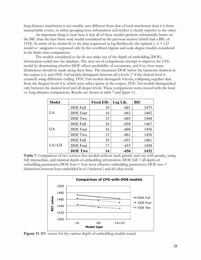
26

long-distance attachment is not notably more different from that of local attachment than it is from unattachable events, so either grouping loses information and neither is clearly superior to the other. An important thing to note here is that all of these models perform substantially better on the BIC than the best finite-state model considered in the previous section (which had a BIC of 1554). In terms of its absolute fit to the data (expressed as log likelihood), the optimal LA + LD model w/ unigrams is surpassed only by the overfitted trigram and scale-degree models considered in the finite-state comparisons. The models considered so far do not make use of the depth-of-embedding (DOE) information coded into the database. The next set of comparisons attempt to improve the CFG model by determining whether DOE affects probability of occurrence, and if so, how many distinctions should be made along these lines. The maximum DOE below the harmonic skeleton in the corpus is 6, and DOE Full models distinguish between all 6 levels (7 if the skeletal level is counted) using difference coding. DOE Four models distinguish 4 levels, collapsing together data from the deepest levels 4-6, which were rather sparse in the corpus. DOE Two models distinguished only between the skeletal level and all deeper levels. These comparisons were crossed with the local vs. long-distance comparisons. Results are shown in table 7 and figure 11.

Model Fixed Effs Log Lik. BIC

LA DOE Full 18 -661 1473 DOE Four 16 -663 1462 DOE Two 13 -665 1444

GA DOE Full 18 -658 1467 DOE Four 16 -660 1456 DOE Two 13 -661 1436

LA+LD DOE Full 19 -651 1461 DOE Four 17 -653 1450 DOE Two 14 -656 1432

Table 7. Comparison of two context-free models without stack penalty and one with penalty, using full, intemediate, and minimal depth-of-embedding information. DOE full = all depth-of-embedding parameters; DOE four = four most effective embedding parameters; DOE two = distinction between least embedded level (‘skeleton’) and all other levels.

Figure 11. BIC scores for the various depth-of-embedding models tested.

1400

1420

1440

1460

1480

1500

LA GA LA+LD

BIC

va

lue

Model type

Comparison of CFG-with-DOE models

DOE Full

DOE Four

DOE Two

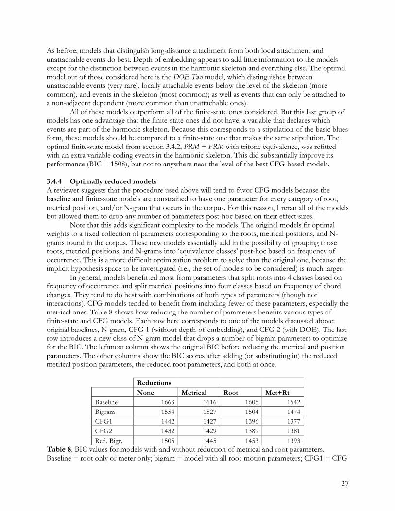
27

As before, models that distinguish long-distance attachment from both local attachment and unattachable events do best. Depth of embedding appears to add little information to the models except for the distinction between events in the harmonic skeleton and everything else. The optimal model out of those considered here is the DOE Two model, which distinguishes between unattachable events (very rare), locally attachable events below the level of the skeleton (more common), and events in the skeleton (most common); as well as events that can only be attached to a non-adjacent dependent (more common than unattachable ones). All of these models outperform all of the finite-state ones considered. But this last group of models has one advantage that the finite-state ones did not have: a variable that declares which events are part of the harmonic skeleton. Because this corresponds to a stipulation of the basic blues form, these models should be compared to a finite-state one that makes the same stipulation. The optimal finite-state model from section 3.4.2, PRM + FRM with tritone equivalence, was refitted with an extra variable coding events in the harmonic skeleton. This did substantially improve its performance (BIC = 1508), but not to anywhere near the level of the best CFG-based models. 3.4.4 Optimally reduced models A reviewer suggests that the procedure used above will tend to favor CFG models because the baseline and finite-state models are constrained to have one parameter for every category of root, metrical position, and/or N-gram that occurs in the corpus. For this reason, I reran all of the models but allowed them to drop any number of parameters post-hoc based on their effect sizes. Note that this adds significant complexity to the models. The original models fit optimal weights to a fixed collection of parameters corresponding to the roots, metrical positions, and N-grams found in the corpus. These new models essentially add in the possibility of grouping those roots, metrical positions, and N-grams into ‘equivalence classes’ post-hoc based on frequency of occurrence. This is a more difficult optimization problem to solve than the original one, because the implicit hypothesis space to be investigated (i.e., the set of models to be considered) is much larger. In general, models benefitted most from parameters that split roots into 4 classes based on frequency of occurrence and split metrical positions into four classes based on frequency of chord changes. They tend to do best with combinations of both types of parameters (though not interactions). CFG models tended to benefit from including fewer of these parameters, especially the metrical ones. Table 8 shows how reducing the number of parameters benefits various types of finite-state and CFG models. Each row here corresponds to one of the models discussed above: original baselines, N-gram, CFG 1 (without depth-of-embedding), and CFG 2 (with DOE). The last row introduces a new class of N-gram model that drops a number of bigram parameters to optimize for the BIC. The leftmost column shows the original BIC before reducing the metrical and position parameters. The other columns show the BIC scores after adding (or substituting in) the reduced metrical position parameters, the reduced root parameters, and both at once.

Reductions None Metrical Root Met+Rt Baseline 1663 1616 1605 1542 Bigram 1554 1527 1504 1474 CFG1 1442 1427 1396 1377 CFG2 1432 1429 1389 1381 Red. Bigr. 1505 1445 1453 1393

Table 8. BIC values for models with and without reduction of metrical and root parameters. Baseline = root only or meter only; bigram = model with all root-motion parameters; CFG1 = CFG

28

with no depth-of-embedding parameters; CFG2 = CFG that distinguishes least embedded (‘skeletal’) events from others; Red. Bigr. = root-motion model with 3 most effective parameters. All of the models considered here are substantially improved by discarding ‘extra’ parameters. Interestingly, finite-state models tend to retain more parameters, and benefit more from them, than CFG models. This is presumably because the CFG approach already indirectly captures some information about relative root frequency (based on the number of rewrite rules required to attach a particular root to the harmonic skeleton) and metrical position (events that are structurally ‘high’ in the syntactic tree tend to occupy prominent metrical positions). In particular, the benefit of depth-of-embedding information completely vanishes when metrical factors are added to the models. Despite the fact that finite-state models have ‘more to gain’ from metrical and root information expressed concisely, CFG models still perform better on the BIC. I take this as a demonstration of the robustness of the CFG results discussed in section 3.4.3. 3.5 A robustness check The methods used here are novel and involve a somewhat idiosyncratic coding of ‘possible’ events. For the simpler models, there is a more straightforward way of coding the corpus without using the notion ‘possible but non-occurring chord change’. It is suggested by Temperley’s (2010) corpus study of metrical structure, where models are assessed using the conditional probabilities of various outcomes under various ways of grouping together the observations in the corpus. In the current study, for instance, grouping observations together using the variable ‘root-motion’ allows us to measure the overall probability of each type of root-motion occurring in the corpus. Assigning to each observation the probability associated with its root-motion type allows us to estimate the likelihood of the entire corpus. And measures of likelihood can be coupled with counts of parameters to derive BIC values for different types of models. Using this approach, we don’t need to distinguish between possible and impossible changes, nor code the data in terms of occurring vs. non-occurring changes. We can simply treat each metrical position in each song as an observation, and assign a probability to each chord in each metrical slot, whether it represents a change in harmony or not. Different ways of grouping the data (root-motion, root only, scale-degree, etc.) will result in different likelihood estimates, corresponding to different models of the corpus. I applied this procedure to some of the simpler models from section 3.4, to check whether the results agree with my novel regression-based methods.

In fitting baseline models, one difficulty immediately arises: there is no equivalent to the original position-only model in this framework. In the original coding, each observation in the data was a chord change, and non-changes were not included. The position-only model therefore took a change in harmony as a given, and modeled whether the attested changes were more likely in some positions than others. The recoding used here includes both changes in harmony and non-changes (prolongations), so the closest equivalent to the position-only model will require a pair of parameters for each metrical position: one parameter for ‘no chord change’ and a second parameter apportioning the probability of change amongst the 11 other chords, without regard to their tonal properties. This is the version of position-only used below.

The comparison between baseline models is shown in table 9. The crossed position x root model is assessed as overly complex here, just as in the original comparison. But in this new version the position model comes out superior to the root-only one. This is readily explained by the difference in coding discussed above. The position model does better on the recoded corpus because once a chord occurs, it’s relatively likely to continue occurring. This probability is ignored by the original coding of the data, which instead focuses in specifically on cases where changes are relatively likely to occur. In other words, metrical information is more useful than root information

29

for describing cases where chords don’t change; but to describe cases where chords do change, root information is more useful.

Model Fixed Effs Log Lik. BIC Rt only 12 -1184 2447 Pos only 49 -1032 2387 Rt * pos 265 -601 2945

Table 9. Comparison of baseline models in the recoded corpus using only metrical position and/or chord root. Rt only = root relative to tonic; Pos only = metrical position; Rt*pos = every root in every metrical position. Table 10 assesses several more complex models that incorporate information about chord changes: the root-motion model, the unigram x root-motion (‘scale degree’) model, and the preceding-root-motion x following-root-motion (trigram) model. As in the original comparison, the simple root-motion model is judged as superior to the more complex interaction models. Perhaps most importantly, it is judged as superior to the baseline models as well.

Model Fixed Effs Log Lik. BIC RM 12 -1022 2122 Uni*RM 133 -941 2756 PRM*FRM 133 -929 2733

Table 10. Comparison of baseline models in the recoded corpus using N-grams. RM = root motion between successive chords; Uni*RM = different root-motion parameters for each different root (‘scale-degree’); PRM*FRM = interactions between preceding and following root motions (trigrams). I take this procedure to show that, at least for models that can be straightforwardly coded in Temperley’s (2010) framework, the results are qualitatively very similar to the novel regression method I’ve used here. The exception is the comparison between baseline models, where the different coding of the data and resultant different nature of the position-only model produce a different result from the original methods. 4 Discussion The preceding sections outlined a theory of the blues, showed that the basic intuitions behind it are sound, formalized various implementations of that basic theory, and compared their performance on modeling the harmonic information in a corpus of blues forms. Several of the conclusions reached along the way have theoretical implications, and I discuss some of them in what follows. 4.1 Root-motion and scale-degree theories Amongst finite-state models of harmonic syntax, root-motion models performed better than ‘scale-degree’ models. In root-motion models, recall, the primary determinant of the probability of a chord sequence is the intervals formed by the roots of successive chords in that sequence. In scale-degree models, each chord may have its own idiosyncratic pattern of characteristic root motions. Tymoczko (2005) concludes, based on a corpus of Bach chorales, that scale-degree models are superior, so the current study is somewhat in tension with those findings. One possible response would be to say that jazz blues is just different than CPP music in this regard. However, I think there are good reasons to doubt that the scale-degree model is superior even for Tymoczko’s corpus.

30

Tymoczko bases his conclusion on comparing a root-motion model where each root motion is either well-formed or ill-formed with a scale-degree model trained on the corpus to assign a probability to each combination of preceding and following chord. Unsurprisingly, the scale-degree model fits the data better. There are at least two problems with this comparison, though. One is that the root-motion model contains 1 free parameter (dominant vs. subdominant motion), while the scale-degree model contains 36. Given that the root-motion model can account for somewhere in the neighborhood of 75% of data points, it seems clear that we’re not getting an enormous return out of adding those additional 35 parameters. This is why principled methods for model comparison are important. A second problem with Tymoczko’s argument is that the bigram model he ends up with, trained on the corpus, is not a very good representation of scale-degree models as a class. These models allow any combination of chords, that is, any cell in the 2x2 transition matrix, to be assigned any probability; while the alternative models claim that certain cells ought to be grouped together. But the transition matrix Tymoczko uses sets 27 of the 49 cells to 0 probability, and clearly displays a tendency for chords on the diagonals representing movement down by 5th and up by 2nd to be more frequent than other root-motion classes.

One plausible explanation of this model is that it is picking up on locally well-formed bigrams by mimicking the root-motion model, and using its large collection of superfluous parameters to ‘soak up’ variance introduced by non-local dependencies. Far from constituting an argument for scale-degree models, I take this to be strong evidence that they get something fundamentally wrong even about the simplified diatonic corpus used by Tymoczko. When an evaluation metric is used that takes the complexity of models into account, as in the current study, it becomes obvious that scale-degree models are wildly overparameterized with respect to corpus data.

While root-motion does seem to be a useful principle for modeling bigrams, it should be noted that the optimal finite-state model in the current study is not a ‘pure’ root-motion model, in Tymoczko’s terms. It benefits from the addition of inherent root frequencies (unigrams). This does not make it a ‘scale-degree’ model in Tymoczko’s sense, because it does not posit different characteristic motions for different roots, but it could be seen as intermediate between a pure root-motion theory and a scale-degree theory. One interpretation of the model is that a chord’s inherent tonal stability with respect to a key (Krumhansl 1990, Lerdahl 2001) or (equivalently) its perceptual distance from the tonic modulates its frequency, largely independent of principles of tonal motion. 4.2 N-gram considerations A type of mixture or ‘look-ahead’ model that considers both preceding and following chords was found to be superior to both bigram and trigram models. Trigram models were found to be far too complex for the data in the corpus.

The inability to produce a useful trigram model of this data is not surprising, as such models often require an enormous amount of data, even when there are relatively few states in the model. Even with a corpus that is an order of magnitude larger than the current one, Granroth-Wilding & Steedman (2014) report no advantage for higher-order Markov models relative to lower-order ones.

The comparison between the pure bigram model and the optimal look-ahead one is a bit harder to interpret. One possibility, given that the best CFG models included long-distance dependencies but also found them to be relatively infrequent, is that the N-gram comparison is making the best of a bad class of models. The pure bigram model can’t capture long-distance effects at all. The trigram model predicts they could be pervasive. And the look-ahead model is able to capture some limited information about trigram dependencies without proliferating parameters for every conceivable dependency.

One might object that the inability to fit a good trigram model (or scale-degree one, for that matter) is due to the relatively small size of the corpus. There are two reasons why I don’t find this

31

line of reasoning persuasive. One is that, no matter how large a corpus of blues forms one could put together, some large number of trigrams (e.g. �2-4-7) are likely to have a frequency indistinguishable from 0. This is inherent to any domain like musical harmony where the vast majority of things that could conceivably happen never actually do. This very basic property of the system suggests in and of itself that lists of sequences of any length (that is, n-grams), are not the right place to start. The most common method for dealing with this in natural language processing is to use backoff models that ‘retreat’ to lower-order Markov processes in the face of sparse data. This method has also had some success with musical corpora (e.g. Pearce & Wiggins 2004) and the general concept bears an interesting complementarity to typical CFG parsers, which first try to parse chords into local groupings, and when they can’t, parse them as dependent on more distant chords.

The second reason why a larger corpus may not be more useful has to do with listeners’ actual exposure to blues forms in the real world. While experienced musicians, like the ones who composed the material in the corpus, may be exposed to thousands of tokens of the blues form over their lifetimes, they will not be exposed to nearly as many distinct types. The forms contained in The Real Book actually appear to me to be nearly comprehensive with respect to what kinds of harmonic elaborations one might find on the 12-bar blues form within the framework of modern jazz, although of course they don’t contain every possible local variation in combination with every other one. Most jazz performers learn the blues form from classic repertoire like that considered here. In other words, this small corpus is not obviously under-representing the type of musical input that a blues learner receives. 4.3 Formal complexity and the syntax of music The BIC criterion used here finds that CFG models are more efficient at describing the blues corpus than comparable finite-state ones. This conclusion holds whether we use the BIC or the less stringent AIC, and whether or not we allow the finite-state models to drop less important parameters. Of course, this is not a standalone proof that harmony must be context-free. The study uses a novel methodology, which can be seen as a limitation. And while the implementations of CFG models here required fewer parameters than their finite-state counterparts, they also require more complexity outside of the regression models. Stating a CFG is more complex than stating a bigram model. For bigram models, one need only say how probable each bigram is. For CFG models, one must determine the relevant rules and the principles that govern their probability of being applied. To implement a CFG also requires a form of memory that a bigram model does not require. So there is a tradeoff here: CFGs require more computational complexity to be implemented, but are able to model the data in the corpus in much more compressed form than finite-state models. In language, this has been taken as a fairly strong argument for CFGs or models of greater complexity. But the really convincing evidence from language, which generally involves either semantic interpretation of syntactic structures or mathematical proofs that hinge on the recursive possibilities of language being infinite, is unlikely to be replicated for music, and is certain not to be found in corpora. The Minimum Description Length (MDL) framework mentioned in section 1.2 may offer a more principled way of thinking about the tradeoff between the general complexity of finding and formulating a CFG and the specific number of parameters it needs to describe any given data set (Grünwald 1996). As Mavromatis (2009) notes, however, the technical challenges in implementing this approach are daunting. And in the end, the assessed complexity of a CFG will depend on what the researcher considers the hypothesis space for CFGs to be like. Stine (2004) points out that MDL methods can and should assess not only models but also the process that led to those models, rewarding theoretically grounded models for their a priori choice of predictors. Using a procedure

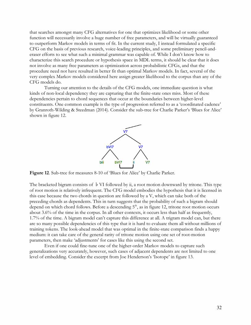
32

that searches amongst many CFG alternatives for one that optimizes likelihood or some other function will necessarily involve a huge number of free parameters, and will be virtually guaranteed to outperform Markov models in terms of fit. In the current study, I instead formulated a specific CFG on the basis of previous research, voice-leading principles, and some preliminary pencil-and-eraser efforts to see what such a minimal grammar was capable of. While I don’t know how to characterize this search procedure or hypothesis space in MDL terms, it should be clear that it does not involve as many free parameters as optimization across probabilistic CFGs, and that the procedure need not have resulted in better fit than optimal Markov models. In fact, several of the very complex Markov models considered here assign greater likelihood to the corpus than any of the CFG models do.

Turning our attention to the details of the CFG models, one immediate question is what kinds of non-local dependency they are capturing that the finite-state ones miss. Most of these dependencies pertain to chord sequences that occur at the boundaries between higher-level constituents. One common example is the type of progression referred to as a ‘coordinated cadence’ by Granroth-Wilding & Steedman (2014). Consider the sub-tree for Charlie Parker’s ‘Blues for Alice’ shown in figure 12.

Figure 12. Sub-tree for measures 8-10 of ‘Blues for Alice’ by Charlie Parker. The bracketed bigram consists of �VI followed by ii, a root motion downward by tritone. This type of root motion is relatively infrequent. The CFG model embodies the hypothesis that it is licensed in this case because the two chords in question are followed by a V, which can take both of the preceding chords as dependents. This in turn suggests that the probability of such a bigram should depend on which chord follows. Before a descending 5th, as in figure 12, tritone root motion occurs about 3.6% of the time in the corpus. In all other contexts, it occurs less than half as frequently, 1.7% of the time. A bigram model can’t capture this difference at all. A trigram model can, but there are so many possible dependencies of this type that it is hard to evaluate them all without millions of training tokens. The look-ahead model that was optimal in the finite-state comparison finds a happy medium: it can take care of the general rarity of tritone motion using one set of root-motion parameters, then make ‘adjustments’ for cases like this using the second set. Even if one could fine-tune one of the higher-order Markov models to capture such generalizations very accurately, however, such cases of adjacent dependents are not limited to one level of embedding. Consider the excerpt from Joe Henderson’s ‘Isotope’ in figure 13.

Discussion

What exactly are the long-distance dependencies at issue here? •!cf. G-W&S: coordinated cadences

e.g. ‘Blues for Alice’ prob. before downward-fifth: 3.6% before other r-m: 1.7%

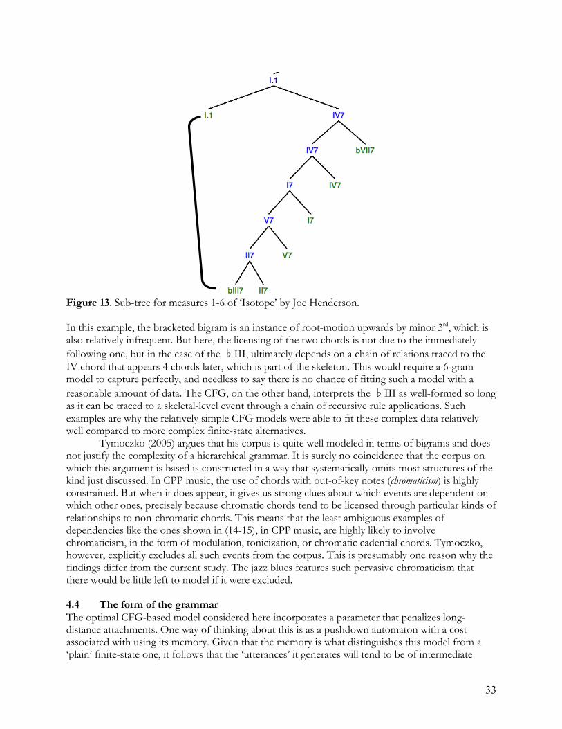
33

Figure 13. Sub-tree for measures 1-6 of ‘Isotope’ by Joe Henderson. In this example, the bracketed bigram is an instance of root-motion upwards by minor 3rd, which is also relatively infrequent. But here, the licensing of the two chords is not due to the immediately following one, but in the case of the �III, ultimately depends on a chain of relations traced to the IV chord that appears 4 chords later, which is part of the skeleton. This would require a 6-gram model to capture perfectly, and needless to say there is no chance of fitting such a model with a reasonable amount of data. The CFG, on the other hand, interprets the �III as well-formed so long as it can be traced to a skeletal-level event through a chain of recursive rule applications. Such examples are why the relatively simple CFG models were able to fit these complex data relatively well compared to more complex finite-state alternatives. Tymoczko (2005) argues that his corpus is quite well modeled in terms of bigrams and does not justify the complexity of a hierarchical grammar. It is surely no coincidence that the corpus on which this argument is based is constructed in a way that systematically omits most structures of the kind just discussed. In CPP music, the use of chords with out-of-key notes (chromaticism) is highly constrained. But when it does appear, it gives us strong clues about which events are dependent on which other ones, precisely because chromatic chords tend to be licensed through particular kinds of relationships to non-chromatic chords. This means that the least ambiguous examples of dependencies like the ones shown in (14-15), in CPP music, are highly likely to involve chromaticism, in the form of modulation, tonicization, or chromatic cadential chords. Tymoczko, however, explicitly excludes all such events from the corpus. This is presumably one reason why the findings differ from the current study. The jazz blues features such pervasive chromaticism that there would be little left to model if it were excluded. 4.4 The form of the grammar The optimal CFG-based model considered here incorporates a parameter that penalizes long-distance attachments. One way of thinking about this is as a pushdown automaton with a cost associated with using its memory. Given that the memory is what distinguishes this model from a ‘plain’ finite-state one, it follows that the ‘utterances’ it generates will tend to be of intermediate

Discussion

Note that these dependencies can go well-beyond trigrams:

e.g. ‘Isotope’

34

complexity between a regular language and a full context-free one. This is somewhat similar to the situation in language. While most linguists agree that natural languages are of at-least context-free complexity, it is entirely obvious that the human linguistic faculty does not utilize the full power of context-free grammars in the way that a machine can. Indeed, it’s fairly easy to come up with even regular languages (generated by a finite-state machine) well beyond the complexity of anything observed in the human domain (see Pullum & Scholz 2009 for discussion and an illustration). And some of the string features that distinguish context-free languages from regular ones, such as the famous multiple center-embedding construction (Chomsky & Miller 1963), clearly pose difficulties for human language processing and are relatively rare in spoken language corpora. So the claim here (and, really, anywhere in the linguistics and cognitive science literature) is not that human languages or musics are exactly like context-free languages or any other level of the Chomsky hierarchy, but simply that they can incorporate properties that distinguish one level of complexity from another. The optimal CFG model treats events in the harmonic ‘skeleton’ as more likely than those embedded under that level, which is unsurprising given that those skeletal events are a criterion for inclusion in the corpus. But the model does not distinguish between events embedded more or less deeply under that skeletal level. This is in part because the relative rarity of deeply embedded events is already coded into the database based on the notion of ‘possible event’ bootstrapped from the corpus. If chords that require 6 levels of embedding are relatively unlikely to occur in any given blues song, they will be relatively unlikely to occur in the corpus at all. They will therefore be unlikely to even be considered as a possibility. What the modeling showed is that, when the opportunity to insert a chord at a deeper level of embedding arises, the probability of choosing to do so does not depend on how many prior embeddings have occurred. This is what we would expect if CFG rules are associated in a straightforward way with a single probability of being applied. The corpus contains events that cannot be assigned a structural description by the CFG developed in section 3, although not a lot of them. This raises the question of what is going on in such cases. One possibility is that the specific CFG used here is too restrictive, and needs to include other rules. Given the relative scarcity of unattachable events and the dangers of overgeneration, however, I favor another interpretation. In the face of overwhelming ‘top-down’ evidence that one is listening to a blues, one is willing to accommodate (or compose) a few aberrant events that don’t straightforwardly fit into the blues schema. An obvious example of this type is Joe Henderson’s ‘Isotope’, which ends with a ‘turnaround’ that progresses to the next chorus’ initial tonic by repeated descending minor-3rd root motion. This is not a typical harmonic device for the blues, nor for the more classic jazz repertoire in general (the song is from the 1960s). By the time this device appears, however, the entire blues skeleton has been outlined and the unusual root motion can be accommodated as an idiosyncratic way of moving towards the initial landmark of the next chorus.

A reviewer suggests that this type of approach could be modeled using a mixture of CFG parameters for ‘canonical’ structural relations and Markov parameters to ‘mop up’ the residue. Fitting a model of this type does indeed improve performance on the BIC: a model identical to the optimal CFG but with up to 3 bigram parameters used to distinguish between more and less likely transitions to unattachable chords reduces the BIC from 1432 to 1427 (for the models in section 3.4.4 with metrical and root information, this addition reduces BIC from 1377 to 1375). This suggests that any approach to composition in terms of hierarchical rules should still allow for the possibility of assessing surface transitions in cases where hierarchical structure is unclear. More generally, the benefit of root-frequency information (and to a much lesser extent, metrical information) in these models suggests that hierarchical syntax is clearly not the only thing that goes into composing a blues form. It was noted in the introduction that if musical syntax is of at least context-free complexity, it would be more similar to language than one might initially have thought. The actual grammar

35

proposed here, however, doesn’t look much like a linguistic one. The CFG notation, using rewrite rules that abstract over categories of terminal elements, is often used in introductory linguistic classes to model fragments of natural language grammars. This notation suggests that only structures corresponding to sequences of licit rewrite rules may be generated. Contemporary work in generative syntax (broadly construed), however, is generally not cast in these phrase-structure terms. Instead, current theories tend to feature relatively free structure building operations coupled with constraints from lexical features and compositional semantics that ‘filter’ out ill-formed instances of particular structures (e.g. Chomsky 1993, Pollard & Sag 1994, Jackendoff 2002). If one is concerned with aligning harmonic theories and linguistic ones, nothing in the grammar proposed here is inconsistent with this view of syntax. One would simply need to rewrite the grammar as a system that can build a relatively unconstrained set of structures, which are then subject to being interpretable by harmonic principles like tritone-equivalence and descending fifth motion. Katz & Pesetsky (2011) argue that even the far more complex Lerdahl & Jackendoff (1983) theory of CPP musical structure could be adapted to such a framework. 4.5 Conclusion While the current study reached some fairly strong conclusions on its own terms, it is probably best viewed as one in a collection of studies using diverse methods, materials, and theories that all converge on the conclusion that musical harmony is a complex, hierarchical syntactic system (Lerdahl & Jackendoff 1983, Lerdahl 2001, Lerdahl & Krumhansl 2007; Steedman 1984, 1996; Johnson-Laird 1991; Smith & Cuddy 2003; Rohrmeier 2011; Katz & Pesetsky 2011). Most notable in this respect is Granroth-Wilding & Steedman’s (2014) corpus study of general jazz-standard harmony (including the 12-bar blues form), which used a larger corpus, a more broadly defined idiom, and very different methods for assessing the performance of generating models. They nonetheless reach a very similar conclusion: the regularities in the corpus are better captured by probabilistic CFGs than by (hidden) Markov models. This is reassuring, because it shows that the conclusion is robust to a number of different analytical and methodological choices. The current study shows that it is possible to conduct such investigations using a single song-form and a fairly small data set, as long as it is supplemented with a way of characterizing ‘possible but non-occurring’ chord changes. The novel method introduced here results in conclusions that are comparable to the works mentioned above, which have reached similar conclusions based on a range of methods including traditional harmonic analysis, perceptual experiments, and corpus studies. Acknowledgments. Many thanks to David Temperley, Dan Shanahan, and two anonymous reviewers for extensive comments on earlier drafts of this paper. Thanks as well to Martin Rohrmeier, Philippe Schlenker, and Mark Steedman for helpful discussion of this project. References Aldwell, E. & C. Schachter. (2010). Harmony and Voice Leading, 4th edition. Boston, MA: Schirmer. Alper, G. (2005). How the flexibility of the twelve-bar blues has helped shape the jazz language.

College Music Symposium 45, 1-12. Anglade, A. & S. Dixon. (2008) Characterisation of harmony with inductive logic programming. In

Proceedings of ISMIR (online). Bates, D., M. Maechler, B. Bolker, S. Walker, R. Christensen, H. Singmann, B. Dai, & G.

Grothendieck. (2015). lme4 v. 1.1-10. R package. Bernstein, L. (1976). The Unanswered Question : Six talks at Harvard. Cambridge, Mass: Harvard

University Press.

36

Broze, Y. & D. Shanahan. (2013). Diachronic Changes in Jazz Harmony: A Cognitive Perspective. Music Perception 31(1), 32-45.

Chomsky, N. (1956). Three models for the description of language. I.R.E. Transactions on Information Theory IT-2, 113-123.

Chomsky, N. (1993). A minimalist program for linguistic theory. In K. Hale and S. Keyser (eds.), The view from Building 20. Cambridge, MA: MIT Press. 1–52.

Chomsky, N. & G. Miller. (1963). Introduction to the formal analysis of natural languages. In R. Luce, R. Bush & E. Galanter (eds.) Handbook of Mathematical Psychology 2. New York: Wiley. 269-323.

Conklin, D. & I. Witten. (1995). Multiple viewpoint systems for music prediction. Journal of New Music Research 24(1), 51-73.

Eigenfeldt, A. & P. Pasquier. (2010). Realtime generation of harmonic progressions using controlled Markov selection. In D. Ventura, A. Pease, R. Pérez, G. Ritchie & T. Veale (eds.), Proceedings of ICCC-X Computational Creativity Conferece: Portugal: University of Coimbra Dept. of Informatics Engineering. 16-25.

Forte, A. & S. Gilbert. (1982). Introduction to Schenkerian Analysis. New York: W.W. Norton. Granroth-Wilding, M. & M. Steedman. (2014). A robust parser-interpreter for jazz chord sequences.

Journal of New Music Research 43(4), 355-374. Grünwald, P. (1996). A Minimal Description Length Approach to Grammar Inference. In S.

Wermter, E. Riloff, and G. Scheler (eds.), Connectionist, Statistical, and Symbolic Approaches to Learning for Natural Language Processing. Berlin: Springer-Verlag, 203-216.

Host, E. & R. Ashley. (2006). Jazz, blues and the language of harmony: Flexibility in online harmonic processing. In Proceedings of ICMPC9.

Jackendoff, R. (2002). Foundations of Language. Oxford University Press. Jaeger, T. (2008). Categorical data analysis: Away from ANOVAs (transformation or not) and

towards logit mixed models. Journal of Memory and Language 59, 434-456. Johnson-Laird, P. (1991). Jazz improvisation: A theory at the computational level. In P. Howell, R.

West, & I. Cross (Eds.), Representing musical structure. San Diego, CA: Academic Press. 291-326 Kadane, J. & N. Lazar. (2004). Methods and criteria for model selection. Journal of the American

Statistical Association 99, 279–290. Kass, R. & A. Raftery. (1995). Bayes factors. Journal of the American Statistical Association 90, 773–795. Katz, J. & D. Pesetsky. (2009). The identity thesis for language and music. Manuscript, MIT. Kernfeld, B. (2006). The Story of Fake Books. Lanham, MD: Scarecrow Press. Koch, L. (1982). Harmonic Approaches to the Twelve-Bar Blues Form. Annual Review of Jazz Studies

1, 559–71. Kostka, S. & D. Payne. (1995) [2013]. Tonal Harmony, 3rd edition [7th edition]. New York: McGraw-Hill. Krumhansl, C. (1990). Cognitive foundations of musical pitch. New York: Oxford University Press. Lerdahl, F. (2001). Tonal pitch space. Oxford: Oxford University Press. Lerdahl, F. & R. Jackendoff. (1983). A generative theory of tonal music. Cambridge, MA: MIT Press. Lerdahl, F. & C. Krumhansl. (2007). Modeling tonal tension. Music Perception 24, 329-366. Lomax, A. (1993). The Land Where the Blues Began. New York: Dell. Love, S. (2012). “Possible Paths”: Schemata of phrasing and melody in Charlie Parker’s Blues. Music

Theory Online 18(3). Mavromatis, P. (2009). Minimun description length modelling of musical structure. Journal of

Mathetmatics and Music 3(3), 117-136. Pachet, F. (1997). Computer Analysis of Jazz Chord Sequences: Is Solar a Blues? in E. Miranda

(Ed.), Readings in Music and Artificial Intelligence. Harwood Academic Publishers. Palmer, R. (1981). Deep Blues. New York: Viking.

37

Patel, A. (2008). Music, language, and the brain. New York: Oxford University Press. Pearce, M. & G. Wiggins. (2004). Improved methods for statistical modeling of monophonic music.

Journal of New Music Research 33, 367-385. Pollard, C. & I. Sag. (1994). Head-driven phrase structure grammar. Chicago: CSLI/University of Chicago

Press Pullum, G. (2010). Creation myths of generative grammar and the mathematics of Syntactic

Structures. In C. Ebert, G. Jäger & J. Michaelis (eds.), Proceedings of the 10th and 11th Biennial Conference on the Mathetmatics of Language. Berlin: Springer. 238-254.

Pullum, G. & B. Scholz. (2009). For universals (but not for finite-state learning) visit the zoo. Behavioral and Brain Sciences 32(5), 466-467.

Quené, H., & van den Bergh, H. (2008). Examples of mixed-effects modeling with crossed random effects and with binomial data. Journal of Memory and Language 59, 413-425.

Rohrmeier, M. (2011). Towards a generative syntax of tonal harmony. Journal of Mathematics and Music 5(1), 35-53.

Rohrmeier, M, Q. Fu & Z. Dienes. (2012). Implicit Learning of Recursive Context-Free Grammars. PLOS One 7(10), e45885.

Shanahan, D. & Y. Broze. (2012). A Diachronic Analysis of Harmonic Schemata in Jazz. In Proceedings of the 12th International Conference of Music Perception and Cognition, 909–918.

Smith, N. & L. Cuddy. (2003). Perceptions of musical dimensions in Beethoven’s Waldstein sonata: An application of tonal pitch space theory. Musicae Scientiae 7(1), 7–34.

Steedman, M. (1984). A generative grammar for jazz chord sequences. Music Perception 2, 52-77. Steedman, M. (1996). The blues and the abstract truth: Music and mental models. In A. Garnham

and J. Oakhill (eds.), Mental models in cognitive science. 305-318. Mahwah, NJ: Erlbaum. Stine, R. (2004). Model Selection Using Information Theory and the MDL Principle. Sociological

Methods & Research 33(2), 230-260. Temperley, D. (2009). A statistical analysis of tonal harmony. HTML manuscript, University of

Rochester. Accessed 9/24/16 at http://davidtemperley.com/kp-stats/ . Temperley, D. (2010). Modeling Common-Practice Rhythm. Music Perception 27(5), 355-376 . Temperley, D. (2011). Composition, perception, and Schenkerian theory. Music Theory Spectrum 33,

146-168. Tymoczko, D. (2005 English translation of 2003 French paper). Progressions fondamentales,

fonctions, degrés: une grammaire de l’harmonie tonale élémentaire. Musurgia 10(3-4). Tymoczko, D. (2010). Local harmonic grammar in Western classical music. Manuscript, Princeton

University. Vrieze, S. (2012). Model selection and psychological theory: A discussion of the differences between

the Akaike Information Criterion (AIC) and the Bayesian Information Criterion (BIC). Psychological Methods 17(2), 228-243.

Young, J. & C. Matheson. (2000). The metaphysics of jazz. Journal of Aesthetics and Art Criticism 58(2), 125-133.

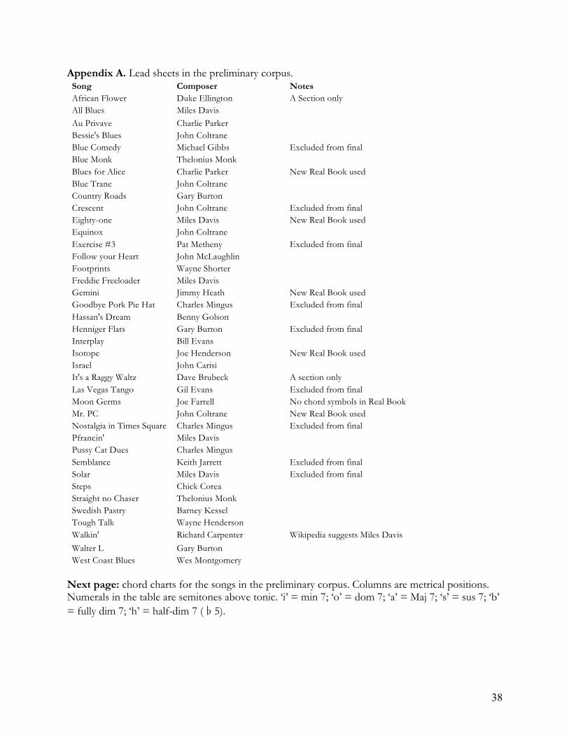
38

Appendix A. Lead sheets in the preliminary corpus. Song Composer Notes African Flower Duke Ellington A Section only All Blues Miles Davis Au Privave Charlie Parker Bessie's Blues John Coltrane Blue Comedy Michael Gibbs Excluded from final Blue Monk Thelonius Monk Blues for Alice Charlie Parker New Real Book used Blue Trane John Coltrane Country Roads Gary Burton Crescent John Coltrane Excluded from final Eighty-one Miles Davis New Real Book used Equinox John Coltrane Exercise #3 Pat Metheny Excluded from final Follow your Heart John McLaughlin Footprints Wayne Shorter Freddie Freeloader Miles Davis Gemini Jimmy Heath New Real Book used Goodbye Pork Pie Hat Charles Mingus Excluded from final Hassan's Dream Benny Golson Henniger Flats Gary Burton Excluded from final Interplay Bill Evans Isotope Joe Henderson New Real Book used Israel John Carisi It's a Raggy Waltz Dave Brubeck A section only Las Vegas Tango Gil Evans Excluded from final Moon Germs Joe Farrell No chord symbols in Real Book Mr. PC John Coltrane New Real Book used Nostalgia in Times Square Charles Mingus Excluded from final Pfrancin' Miles Davis Pussy Cat Dues Charles Mingus Semblance Keith Jarrett Excluded from final Solar Miles Davis Excluded from final Steps Chick Corea Straight no Chaser Thelonius Monk Swedish Pastry Barney Kessel Tough Talk Wayne Henderson Walkin' Richard Carpenter Wikipedia suggests Miles Davis Walter L Gary Burton West Coast Blues Wes Montgomery

Next page: chord charts for the songs in the preliminary corpus. Columns are metrical positions. Numerals in the table are semitones above tonic. ‘i’ = min 7; ‘o’ = dom 7; ‘a’ = Maj 7; ‘s’ = sus 7; ‘b’ = fully dim 7; ‘h’ = half-dim 7 (�5).

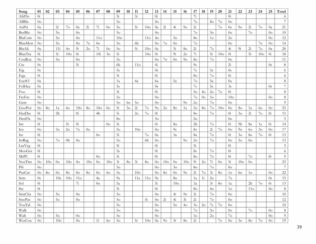
39

Song 01 02 03 04 05 06 07 08 09 10 11 12 13 14 15 16 17 18 19 20 21 22 23 24 25 Total AfrFlo 0i 5i 3i 0i 7i 0i 6 AllBlu 0o 5o 0o 7o 8o 7o 0o 7 AuPri 0a 2i 7o 0a 2i 7i 0o 5o 5i 10o 0a 2i 4i 9o 2i 7o 0a 9o 2i 7o 0a 21 BesBlu 0o 5o 0o 5o 0o 7o 5o 0o 7o 0o 10 BluCom 0o 5o 0o 11o 10o 11o 4o 3o 8o 1o 2o 0o 12 BlueMon 0o 5o 0o 7o 0o 5o 6b 0o 7o 0o 7o 0o 7o 0o 14 BluAli 0a 11i 4o 9i 2o 7i 0o 5o 5i 10o 0a 3i 8o 2i 7o 4i 9i 2i 7o 0a 20 BlueTra 0i 5i 10o 0i 10i 3o 5i 10o 0i 9i 2o 7i 5i 10o 0i 5i 10o 0i 18 CouRoa 0o 5o 0o 5o 0o 7o 0o 9o 8o 7o 0o 11 Cre 0s 5i 6h 11o 4i 9s 2i 0s 8 Eig 0s 5s 0s 7s 5s 0s 6 Equ 0i 5i 0i 8o 7o 0i 6 Exe#3 0a 1a 4a 6a 5a 7o 5a 0a 8 FolHea 0s 5s 0s 7s 5s 3s 0s 7 Foo 0i 5i 0i 5o 4o 2o 7o 0i 8 FreFre 0o 5o 0o 7o 0o 5o 10o 0o 8 Gem 0o 5o 6o 5o 0o 9o 2o 7o 0o 9 GooPor 0o 8o 1a 6o 10o 8o 10o 0o 5i 3o 2i 7o 9o 2o 8o 1a 5o 8o 7o 10o 0o 8o 1a 6o 0o 25 HasDre 0i 2b 0i 4b 5i 2o 7o 0i 8o 7o 0i 3o 2i 7o 0i 15 HenFla 0o 8o 5o 2o 0o 5 Int 0i 5i 0i 0o 5i 0i 8o 2h 7o 0i 9h 8a 1a 0i 14 Iso 0o 3o 2o 7o 0o 5o 10o 0o 9s 8s 2i 7o 0o 9o 6o 3o 0o 17 Isr 0i 0o 5i 7o 0a 3a 8a 7o 0i 3o 8o 7o 0i 13 ItsRag 0o 7o 0b 0o 5o 6b 0o 9o 2o 7o 0o 5o 0o 13 LasVeg 0i 5i 0i 5i 0i 5 MooGer 0i 5s 0i 8s 7o 0i 6 MrPC 0i 0o 5i 0i 8o 7o 0i 7o 0i 9 NosTim 0o 10o 0o 10o 0o 10o 0o 10o 3i 8o 3i 8o 0o 10o 0o 10o 9i 2o 7i 0o 5i 10o 0o 23 Pfr 0o 5o 0o 3o 8o 7o 0o 7 PusCat 0o 8o 0o 8o 0o 8o 0o 6o 5o 10o 0o 8o 0o 9o 2i 7o 3i 8o 1o 6o 1o 0o 22 Sem 0s 10a 10o 11o 4a 9a 11a 11o 9a 8o 1a 1i 2o 7o 0s 15 Sol 0i 7i 0o 5a 5i 10o 3a 3i 8o 1a 2h 7o 0i 13 Ste 0i 5i 0i 8o 4o 1o 11o 0o 8 StraCha 0o 5o 0o 5o 0o 4i 9o 2i 7o 0o 10 SwePas 0o 5o 0o 5o 5i 0o 2i 4i 3i 2i 7o 0o 12 TouTal 0o 5o 0o 5o 4o 3o 2o 7s 7o 0o 10 Walk 0o 5o 0o 7o 5o 0o 7o 0o 8 Walt 0o 5o 0o 5o 0o 1o 2o 7o 0o 9 WesCoa 0o 10o 0o 1i 6o 5o 5i 10o 0a 9o 3i 8o 2i 7o 0o 3o 8o 7o 0o 19

40