Embed Size (px)
Citation preview

Running head: Factor Scores, Structure Coefficients, and Communality Coefficients 1
Factor Scores, Structure Coefficients, and Communality Coefficients
Fara Goodwyn
Texas A&M University
Paper presented at the annual meeting of the Southwest Educational Research Association, New
Orleans, February 2, 2012.

Running head: Factor Scores, Structure Coefficients, and Communality Coefficients 2
Abstract
This paper presents heuristic explanations of factor scores, structure coefficients, and communality
coefficients. Common misconceptions regarding these topics are clarified. In addition, (a) the
regression (b) Bartlett, (c) Anderson-Rubin, and (d) Thompson methods for calculating factor
scores are reviewed. Syntax necessary to execute all four methods are provided.
Keywords: Anderson-Rubin method, Bartlett method, communality coefficients, factor
scores, regression method, structure coefficients, Thompson method

Running head: Factor Scores, Structure Coefficients, and Communality Coefficients 3
Factor Scores, Structure Coefficients, and Communality Coefficients
An understanding of the terminology and principles underlying factor scores,
structure coefficients, and communality coefficients is critical to correctly interpreting
factor analytic results (Wells, 1999). This paper reviews factor scores, structure
coefficients, and communality coefficients while clarifying misconceptions regarding
these concepts. Misconceptions are common throughout factor analysis in part due to
multiple terms assigned to the same statistical concepts. Garbarino (1996) elaborates
on this problem:
For example, we call the same systems of weights "equations" in regression,
"factors" in factor analysis, "functions" or "rules" in discriminant analysis, and
"functions" in canonical correlational analysis. We call the weights themselves
"beta" weights in regression, "pattern coefficients" in factor analysis, and
"standardized function coefficients" in discriminant analysis or canonical
correlation analysis. The synthetic scores are called "yhat" in regression,
"factor scores" in factor analysis, "discriminant scores" in discriminant
analysis, and "canonical function (or variate) scores" in canonical correlation
analysis. (p. 3)
After reviewing foundational concepts, the (a) regression, (b) Bartlett, (c)
Anderson-Rubin, and (d) Thompson factor score estimation methods are compared.
Differences in factor scores resulting from principal components or principal axes
extraction are explored. All heuristic explanations utilize six variables from the
Holzinger and Swineford (1939) data set. Table 1 presents the variables along with
their respective variable labels. These variables were selected due to the appearance of

Running head: Factor Scores, Structure Coefficients, and Communality Coefficients 4
two obvious underlying constructs (i.e., two factors – speed and memory). Finally, factor
scores are used in heuristic explanations of structure and communality coefficients.
Table 1
Variable Labels
Variable Label
t10 Speeded Addition Test
t11 Speeded Code Test – Transform Shapes into Alpha with Code
t12 Speeded Counting of Dots in Shape
t15 Memory of Target Numbers
t16 Memory of Target Shapes
t17 Memory of Object – Number Association Targets
Foundational Concepts
Matrix of Bivariate Associations
The matrix of bivariate associations created from measured variable data is the focus of
factor analysis. The Pearson product-moment bivariate correlation matrix is the most utilized
matrix of bivariate associations. In fact, it is the default bivariate correlation matrix in most
statistical software packages. Table 2 presents the Pearson product-moment bivariate correlation
matrix for the selected variables.
Table 2
Pearson Product-Moment Bivariate Correlation Matrix
Variable t10 t11 t12 t15 t16 t17
t10 1.000 0.447 0.487 0.109 0.117 0.331
t11 0.447 1.000 0.398 0.140 0.305 0.344
t12 0.487 0.398 1.000 0.078 0.146 0.230
t15 0.109 0.140 0.078 1.000 0.338 0.305
t16 0.117 0.305 0.146 0.338 1.000 0.259
t17 0.331 0.344 0.230 0.305 0.259 1.000

Running head: Factor Scores, Structure Coefficients, and Communality Coefficients 5
Factor Scores
Understandably, factors and factor scores are often confused. Factor analysis consolidates
original measured variables into factors (i.e., latent variables), maximizing original data information
(Hetzel, 1996; Thompson, 2004). Factors provide a means “for determining if there are a small
number of underlying constructs which might account for the main sources of variation in
such a complex set of correlations ” (i.e., variables may not be measuring different constructs;
Stevens, 1996, p. 362). Factors, found in the output file of SPSS, are specific to measured variables
as seen in Table 3.
Table 3
Rotated Factor Matrix for Regression Method using Principal Axes Extraction
Factor
Variable 1 2
t10 0.744 0.095
t11 0.584 0.297
t12 0.634 0.080
t15 0.037 0.594
t16 0.140 0.557
t17 0.354 0.441
Factor scores, found in the data file of SPSS, can be used in utilized in
subsequent analyses. Table 4 presents factor scores derived from the regression method.
Notice factor scores are specific to individual participants, not measured variables. In
regression, the analogous terminology for latent scores is yhat scores (Thompson, 2004).
Running head: Factor Scores, Structure Coefficients, and Communality Coefficients 6
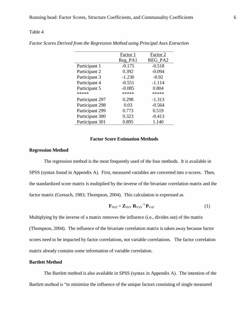
Table 4
Factor Scores Derived from the Regression Method using Principal Axes Extraction
Factor 1
Reg_PA1
Factor 2
REG_PA2
Participant 1 -0.175 -0.518
Participant 2 0.392 -0.094
Participant 3 -1.230 -0.92
Participant 4 -0.551 -1.114
Participant 5 -0.085 0.804
***** ***** *****
Participant 297 0.298 -1.313
Participant 298 0.03 -0.564
Participant 299 0.773 0.519
Participant 300 0.323 -0.413
Participant 301 0.895 1.140
Factor Score Estimation Methods
Regression Method
The regression method is the most frequently used of the four methods. It is available in
SPSS (syntax found in Appendix A). First, measured variables are converted into z-scores. Then,
the standardized score matrix is multiplied by the inverse of the bivariate correlation matrix and the
factor matrix (Gorsuch, 1983; Thompson, 2004). This calculation is expressed as
FNxF = ZNxV RVxV-1
PVxF (1)
Multiplying by the inverse of a matrix removes the influence (i.e., divides out) of the matrix
(Thompson, 2004). The influence of the bivariate correlation matrix is taken away because factor
scores need to be impacted by factor correlations, not variable correlations. The factor correlation
matrix already contains some information of variable correlation.
Bartlett Method
The Bartlett method is also available in SPSS (syntax in Appendix A). The intention of the
Bartlett method is “to minimize the influence of the unique factors consisting of single measured

Running head: Factor Scores, Structure Coefficients, and Communality Coefficients 7
variables not usually extracted in the analysis” (Thompson, 2004, p. 44). Bartlett’s method
minimizes the sums of squares of factors across a set of variables using least squares procedures
(Bartlett, 1937). These procedures result in a high correlation between factor scores and their
respective factors (Gorsuch, 1983).
Anderson-Rubin Method
The Anderson-Rubin method (available in SPSS, syntax found in Appendix A) also
produces factor scores with high correlations with their respective factors. Unlike the Bartlett
method, factor scores produced by the Anderson-Rubin method are always perfectly uncorrelated
(Anderson & Rubin, 1956; Thompson, 2004; Wells, 1999).
Thompson Method
The Thompson method can be performed using SPSS with syntax provided in Appendix A.
Standard point-and-click methods within SPSS are not available for this method. The Thompson
method produces standardized (i.e., standard deviations of 1), non-centered (i.e., non-zero means)
factor scores comparable across factors. As Thompson (1993) states, “sometimes we wish to
compare means on factor scores across factors to make some judgment regarding the relative
importance of given factors” (p. 1129). Factor scores produced by the regression, Bartlett, and
Anderson-Rubin methods are not capable of such a comparison (Thompson, 1993).
There are three steps for calculating factor scores in the Thompson method. First, variables
are converted to z-scores. Second, variable means provided in SPSS descriptive statistics output are
added to the z-scores. Third, the factor score coefficient matrix (also provided in SPSS output) is
applied to the newly standardized, non-centered scores. The third step is expressed by the following
formula:
W = RVxV-1
PVxF (2)

Running head: Factor Scores, Structure Coefficients, and Communality Coefficients 8
Variable mean values and weight values obtained from the factor score coefficient matrix are
directly entered in the syntax as shown in Appendix A.
Table 5 presents a comparison of factor scores derived from the regression method (using
principal components) to factor scores derived from the Thompson method. Unlike factor scores
produced by the regression method, factors scores produced by the Thompson method allow the
researcher to see an overall higher rating on factor one, speed.
Table 5
Factor Scores: Regression and Thompson Methods
Regression Thompson
Participant REG_PC1 REG_PC2 BTscr1 BTscr2
Participant 1 -0.028 -0.780 92.475 79.976 Participant 2 0.699 -0.302 93.203 80.453 Participant 3 -1.516 -1.039 90.985 79.717 Participant 4 -0.420 -1.531 92.082 79.225 Participant 5 -0.034 1.081 92.471 81.837
*****
Participant 297 0.304 -1.723 92.806 79.034 Participant 298 -0.038 -0.687 92.464 80.070 Participant 299 1.078 0.375 93.582 81.131 Participant 300 0.316 -0.481 92.819 80.275 Participant 301 1.328 1.318 93.833 82.073
Extraction Methods
Principal Components Extraction Method
Principal components factor extraction always produces identical results for the regression,
Bartlett, and Anderson-Rubin factor estimation methods. In fact, the comparison made in Table 5
could have been demonstrated with the Bartlett or Anderson-Rubin methods in place of the
regression method as these factor estimation methods all yield the same results. Table 6 presents
selected factor scores derived from the regression, Bartlett, and Anderson-Rubin methods.

Running head: Factor Scores, Structure Coefficients, and Communality Coefficients 9
Table 6
Factor Scores with Principal Component Extraction for Regression, Bartlett, and Anderson-Rubin
Regression Bartlett Anderson-Rubin
Participant REG_PC1 REG_PC2 BART_PC1 BART_PC2 AR_PC1 AR_PC2
Participant 1 -0.028 -0.780 -0.028 -0.780 -0.028 -0.780
Participant 2 0.699 -0.302 0.699 -0.302 0.699 -0.302
Participant 3 -1.516 -1.039 -1.516 -1.039 -1.516 -1.039
Participant 4 -0.420 -1.531 -0.420 -1.531 -0.420 -1.531
Participant 5 -0.034 1.081 -0.034 1.081 -0.034 1.081
*****
Participant 297 0.304 -1.723 0.304 -1.723 0.304 -1.723
Participant 298 -0.038 -0.687 -0.038 -0.686 -0.038 -0.686
Participant 299 1.078 0.375 1.078 0.375 1.078 0.375
Participant 300 0.316 -0.481 0.316 -0.481 0.316 -0.481
Participant 301 1.328 1.318 1.328 1.318 1.328 1.318
Principal Axes Extraction Method
Unlike the principal components method, the principal axes factor extraction method
produces different factor score values dependent upon the factor extraction method selected. Table
7 presents factor scores using principal axes extraction with the regression, Bartlett, and Anderson-
Rubin methods.
Table 7
Factor Scores with Principal Axes Extraction for Regression, Bartlett, and Anderson-Rubin
Regression Bartlett Anderson-Rubin
Participant REG_PA1 REG_PA2 BART_PA1 BART_PA2 AR_PA1 AR_PA2
Participant 1 0-.175 -0.518 -0.103 -0.915 -0.150 -0.686
Participant 2 0.392 -0.094 0.604 -0.289 0.485 -0.172
Participant 3 -1.230 -0.924 -1.533 -1.360 -1.378 -1.116
Participant 4 -0.551 -1.114 -0.477 -1.914 -.533 -1.453
Participant 5 -0.085 0.804 -0.338 1.512 -0.177 1.098
*****
Participant 297 0.298 -1.313 0.798 -2.512 0.493 -1.808
Participant 298 0.032 -0.564 0.203 -1.051 0.097 -0.766
Participant 299 0.773 0.519 0.965 0.736 0.860 0.614
Participant 300 0.323 -0.413 0.597 -0.856 0.440 -0.594
Participant 301 0.895 1.140 0.993 1.860 0.962 1.450

Running head: Factor Scores, Structure Coefficients, and Communality Coefficients 10
Principal Components vs. Principal Axes
Factors are uncorrelated upon initial extraction. Factors remain uncorrelated if they are
orthogonally rotated or not rotated at all (Wells, 1999). The current analysis utilized Varimax
rotation, an orthogonal rotation method; therefore, the two factors remained perfectly
uncorrelated.
Uncorrelated factors do not always result in uncorrelated factor scores. When utilizing an
orthogonal rotation method, the principal component extraction method has the added benefit of
producing perfectly uncorrelated factors and perfectly uncorrelated factor scores. Principal axes
extraction method only results in uncorrelated factor scores when the Anderson-Rubin method is
used.
Factor Structure Coefficients
Throughout the General Linear Model, bivariate correlations between measured and
latent variables are called structure coefficients. Factor structure coefficients, the Pearson r
correlation between measured variables and latent factor scores, are equal to pattern coefficients
(i.e., weights) when factors remain uncorrelated (Thompson, 2004). As noted above, principal
component analysis always produces uncorrelated factor scores when using an orthogonal
rotation. Not surprisingly, Table 8 (the rotated factor matrix, also correctly referred to as the factor
pattern coefficient matrix) and Table 9 (factor structure coefficients) are equal across variables using
principal component extraction. Because the values are equal, the factor structure coefficients are
more accurately referred to as pattern/structure coefficients.

Running head: Factor Scores, Structure Coefficients, and Communality Coefficients 11
Table 8
Rotated Factor Matrix for Regression Method using Principal Component Extraction
Factor
Variable 1 2
t10 0.823 0.058
t11 0.706 0.824
t12 0.793 0.006
t15 -0.026 0.807
t16 0.117 0.747
t17 0.420 0.549
Table 9
Factor Structure Coefficients for Regression Method using Principal Component Extraction
Factor
Variable 1 2
t10 0.823 0.058
t11 0.706 0.824
t12 0.793 0.006
t15 -0.026 0.807
t16 0.117 0.747
t17 0.420 0.549
In contrast, the pattern coefficient values in the factor matrix produced using principal axes
extraction (see Table 3) does not equal factor structure coefficient values found in Table 10.
Researchers must analyze both pattern coefficients and structure coefficients in this scenario
(Thompson, 2004).

Running head: Factor Scores, Structure Coefficients, and Communality Coefficients 12
Table 10
Factor Structure Coefficient for Regression Method using Principal Axes Extraction
Factor
Variable 1 2
t10 0.885 0.127
t11 0.694 0.398
t12 0.754 0.108
t15 0.045 0.796
t16 0.166 0.748
t17 0.885 0.127
Communality Coefficients
A communality coefficient (h2) is “a statistic in a squared metric indicating how much of
the variance in a measured variable the factors as a set can reproduce, or conversely, how much of
the variance of a given measured variable was useful in delineating the factors as a set” (Thompson,
2004, p. 179). Communality coefficients are specific to measured variables. The equation for h2
with uncorrelated factors is
h2 = ∑ rs
2 (3)
and is analogous to
R2 = ∑ rs
2 (4)
for uncorrelated factors. Therefore, h2 is the R
2 effect size for uncorrelated factors. A different
formula, which is beyond the scope of this paper, exists for correlated factors (Thompson, 2004).
Communality coefficients are readily available in the output of SPSS. The communality
coefficient for t10 is 0.681. For heuristic purposes, the communality coefficient will be calculated
for t10 using Equation 3. Structure coefficient values (Pearson r values as previously explained) for
t10 are 0.823 and 0.058 for the first and second factor respectively. When these values are squared,
as directed by Equation 3, the resulting values are 0.677 and 0.003. These squared factor structure

Running head: Factor Scores, Structure Coefficients, and Communality Coefficients 13
coefficients for each variable are summed across factors. The sum for t10 is 0.680 which only
varies from the communality coefficient produced by SPSS due to rounding error. The factors
reproduced 68% of the variance of the measured variable t10. The syntax to produce this R2 type
effect size is available in Appendix B.
Conclusion
Correct interpretation of factor analytic results relies on a solid understanding of factor
scores, structure coefficients, and communality coefficients and related terminology. Take away
points from this paper include:
Principal components extraction results in identical factor scores for the regression, Bartlett,
and Anderson-Rubin methods.
The Thompson method alone allows for comparison of factors scores across factors for the
dataset as a whole.
Uncorrelated factors may or may not have uncorrelated factor scores.
Structure coefficients are bivariate correlation coefficients between the measured variables
with the factor scores.
Communality coefficients (h2) can be the R
2 effect size.

Running head: Factor Scores, Structure Coefficients, and Communality Coefficients 14
References
Anderson, T.W., & Rubin, H. (1956). Statistical inference in factor analysis. Proceedings of the
Third Berkeley Symposium on Mathematical Statistics and Probability, 5, 111-150.
Bartlett, M.S. (1937). The statistical conception of mental factors. British Journal of Psychology,
28, 97-104.
Garbarino, J. J. (1996). Alternate ways of computing factor scores. Paper presented at the
annualmeeting of the Southwest Educational Research Association, New Orleans.
Gorsuch, R.L. (1983). Factor analysis (2nd
ed.). Hillsdale, NJ:Erlbaum.
Hetzel, R.D. (1996). A primer on factor analysis with comments on analysis and interpretation
patterns. In B. Thompson (Ed.), Advances in social science methodology (Vol. 4, pp. 175-
206). Greenwich, CT: JAI Press.
Holzinger, K.J., & Swineford, F. (1939). A study in factor analysis: The stability of a bi-factor
solution (No. 48). Chicago: University of Chicago. (data on pp. 81-91)
Stevens, J. (1996). Applied multivariate statistics for the social sciences. Mahway, NJ: Lawrence
Erlbaum.
Thompson, B. (1992). DISCSTRA: A computer program that computes bootstrap resampling
estimates of descriptive discriminant analysis function and structure coefficients and group
centroids. Educational and Psychological Measurement, 52, 905-911.
Thompson, B. (1993). Calculation of standardized, noncentered factor scores: An
alternative to conventional factor socres. Perceptual and Motor Skills, 77,
1128-1130.

Running head: Factor Scores, Structure Coefficients, and Communality Coefficients 15
Thompson, B. (2000). Canonical correlation analysis. In L. Grimm & P. Yarnold (Eds.), Reading
and understanding more multivariate statistics (pp. 285-316). Washington, DC: American
Psychological Association.
Thompson, B. (2004). Exploratory and confirmatory factor analysis: Understanding
concepts and applications. Washington, DC: American Psychological
Association.
Wells, R.D. (1999). Factor scores and factor structure communality coefficients. In B. Thompson
(Ed.), Advances in social science methodology (Vol. 5, pp. 123-138). Stamford, CT: JAI
Press.
Running head: Factor Scores, Structure Coefficients, and Communality Coefficients 16
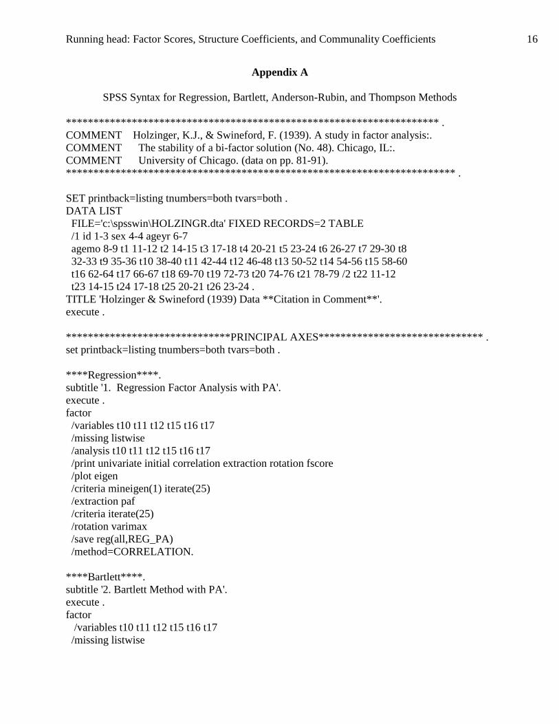
Appendix A
SPSS Syntax for Regression, Bartlett, Anderson-Rubin, and Thompson Methods
******************************************************************** .
COMMENT Holzinger, K.J., & Swineford, F. (1939). A study in factor analysis:.
COMMENT The stability of a bi-factor solution (No. 48). Chicago, IL:.
COMMENT University of Chicago. (data on pp. 81-91).
*********************************************************************** .
SET printback=listing tnumbers=both tvars=both .
DATA LIST
FILE='c:\spsswin\HOLZINGR.dta' FIXED RECORDS=2 TABLE
/1 id 1-3 sex 4-4 ageyr 6-7
agemo 8-9 t1 11-12 t2 14-15 t3 17-18 t4 20-21 t5 23-24 t6 26-27 t7 29-30 t8
32-33 t9 35-36 t10 38-40 t11 42-44 t12 46-48 t13 50-52 t14 54-56 t15 58-60
t16 62-64 t17 66-67 t18 69-70 t19 72-73 t20 74-76 t21 78-79 /2 t22 11-12
t23 14-15 t24 17-18 t25 20-21 t26 23-24 .
TITLE 'Holzinger & Swineford (1939) Data **Citation in Comment**'.
execute .
******************************PRINCIPAL AXES****************************** .
set printback=listing tnumbers=both tvars=both .
****Regression****.
subtitle '1. Regression Factor Analysis with PA'.
execute .
factor
/variables t10 t11 t12 t15 t16 t17
/missing listwise
/analysis t10 t11 t12 t15 t16 t17
/print univariate initial correlation extraction rotation fscore
/plot eigen
/criteria mineigen(1) iterate(25)
/extraction paf
/criteria iterate(25)
/rotation varimax
/save reg(all,REG_PA)
/method=CORRELATION.
****Bartlett****.
subtitle '2. Bartlett Method with PA'.
execute .
factor
/variables t10 t11 t12 t15 t16 t17
/missing listwise

Running head: Factor Scores, Structure Coefficients, and Communality Coefficients 17
/analysis t10 t11 t12 t15 t16 t17
/print univariate initial correlation extraction rotation fscore
/plot eigen
/criteria mineigen(1) iterate(25)
/extraction paf
/criteria iterate(25)
/rotation varimax
/save bart(all, BART_PA)
/method=CORRELATION.
****Anderson-Rubin****.
subtitle '3. Anderson-Rubin Method with PA'.
execute .
factor
/variables t10 t11 t12 t15 t16 t17
/missing listwise
/analysis t10 t11 t12 t15 t16 t17
/print univariate initial correlation extraction rotation fscore
/plot eigen
/criteria mineigen(1) iterate(25)
/extraction paf
/criteria iterate(25)
/rotation varimax
/save ar(all, AR_PA)
/method=CORRELATION.
*************************** PRINCIPAL COMPONENT***************************
.
****Regression*****.
subtitle '4. Regression Factor Analysis with PC'.
execute .
factor
/variables t10 t11 t12 t15 t16 t17
/missing listwise
/analysis t10 t11 t12 t15 t16 t17
/print univariate initial correlation extraction rotation fscore
/plot eigen
/criteria mineigen(1) iterate(25)
/extraction pc
/criteria iterate(25)
/rotation varimax
/save reg(all, REG_PC)
/method=CORRELATION.
****Bartlett****.
subtitle '5. Bartlett Method with PC'.

Running head: Factor Scores, Structure Coefficients, and Communality Coefficients 18
execute .
factor
/variables t10 t11 t12 t15 t16 t17
/missing listwise
/analysis t10 t11 t12 t15 t16 t17
/print univariate initial correlation extraction rotation fscore
/plot eigen
/criteria mineigen(1) iterate(25)
/extraction pc
/criteria iterate(25)
/rotation varimax
/save bart(all, BART_PC)
/method=CORRELATION.
****Anderson-Rubin****.
subtitle '6. Anderson-Rubin Method with PC'.
execute .
factor
/variables t10 t11 t12 t15 t16 t17
/missing listwise
/analysis t10 t11 t12 t15 t16 t17
/print univariate initial correlation extraction rotation fscore
/plot eigen
/criteria mineigen(1) iterate(25)
/extraction pc
/criteria iterate(25)
/rotation varimax
/save ar(all, AR_PC)
/method=CORRELATION.
****************************THOMPSON METHOD*****************************
.
descriptives variables=t10 t11 t12 t15 t16 t17/save .
subtitle '7. Thompson Method'.
****(1) compute z scores**** .
**** (2) add original measured variable means back onto z scores **** .
compute ct10 = zt10 + 96.28 .
compute ct11 = zt11 + 69.16 .
compute ct12 = zt12 + 110.54 .
compute ct15 = zt15 + 90.01 .
compute ct16 = zt16 + 102.52 .
compute ct17 = zt17 + 8.23 .
print formats zt10 to ct17 (F7.2) .
list variables=id zt10 to ct17/cases=10 .
descriptives variables= zt10 to ct17 .
Running head: Factor Scores, Structure Coefficients, and Communality Coefficients 19
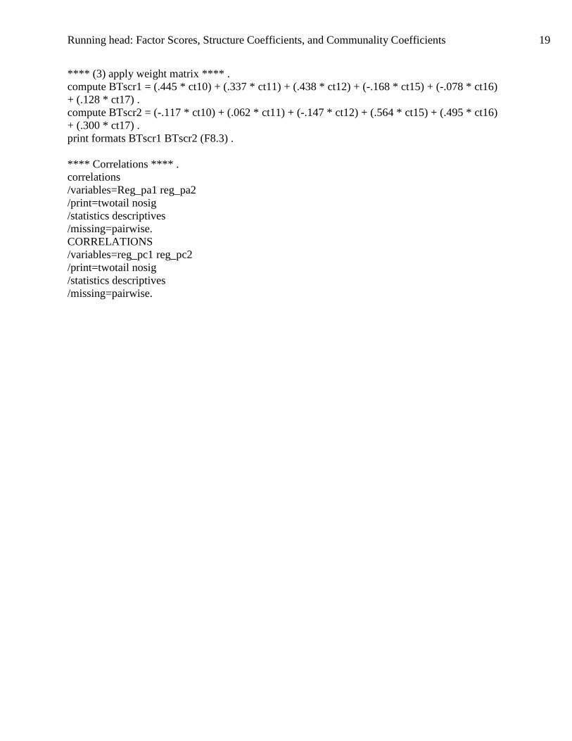
**** (3) apply weight matrix **** .
compute BTscr1 = (.445 * ct10) + (.337 * ct11) + (.438 * ct12) + (-.168 * ct15) + (-.078 * ct16)
+ (.128 * ct17) .
compute BTscr2 = (-.117 * ct10) + (.062 * ct11) + (-.147 * ct12) + (.564 * ct15) + (.495 * ct16)
+ (.300 * ct17) .
print formats BTscr1 BTscr2 (F8.3) .
**** Correlations **** .
correlations
/variables=Reg_pa1 reg_pa2
/print=twotail nosig
/statistics descriptives
/missing=pairwise.
CORRELATIONS
/variables=reg_pc1 reg_pc2
/print=twotail nosig
/statistics descriptives
/missing=pairwise.

Running head: Factor Scores, Structure Coefficients, and Communality Coefficients 20
Appendix B
SPSS Syntax for Multiple R Squared
**** Calculate Multiple R Squared type effect size **** .
regression variables=reg_pc1 to reg_pc2
t10 t11 t12 t15 t16 t17 / dependent = t10 /
enter reg_pc1 to reg_pc2.
regression variables=reg_pc1 to reg_pc2
t10 t11 t12 t15 t16 t17 / dependent = t11 /
enter reg_pc1 to reg_pc2.
regression variables=reg_pc1 to reg_pc2
t10 t11 t12 t15 t16 t17 / dependent = t12 /
enter reg_pc1 to reg_pc2.
regression variables=reg_pc1 to reg_pc2
t10 t11 t12 t15 t16 t17 / dependent = t15 /
enter reg_pc1 to reg_pc2.
regression variables=reg_pc1 to reg_pc2
t10 t11 t12 t15 t16 t17 / dependent = t16 /
enter reg_pc1 to reg_pc2.
regression variables=reg_pc1 to reg_pc2
t10 t11 t12 t15 t16 t17 / dependent = t17 /
enter reg_pc1 to reg_pc2.