Embed Size (px)
Citation preview
Running Head: CORRELATION WITH NON-NORMAL DATA 1
Testing the Significance of a Correlation with Non-normal Data: Comparison of Pearson,
Spearman, Transformation, and Resampling Approaches
Anthony J. Bishara and James B. Hittner
College of Charleston
Author Note
Anthony J. Bishara, Department of Psychology, College of Charleston.
James B. Hittner, Department of Psychology, College of Charleston.
We thank William Beasley and Martin Jones for helpful feedback on this project. We
also thank Clayton McCauley and Allan Strand for assistance with the College of Charleston
Daito cluster.
Correspondence concerning this article should be addressed to Anthony J. Bishara, Dept.
of Psychology, College of Charleston, 66 George St., Charleston, SC 29424. E-mail:
Reference:
Bishara, A. J., & Hittner, J. B. (2012). Testing the significance of a correlation with non-normal
data: Comparison of Pearson, Spearman, transformation, and resampling approaches.
Psychological Methods, 17, 399-417. doi:10.1037/a0028087
CORRELATION WITH NON-NORMAL DATA 2
Abstract
It is well known that when data are non-normally distributed, a test of the significance of
Pearson's r may inflate Type I error rates and reduce power. Statistics textbooks and the
simulation literature provide several alternatives to Pearson’s correlation. However, the relative
performance of these alternatives has been unclear. Two simulation studies were conducted to
compare 12 methods, including Pearson, Spearman's rank-order, transformation, and resampling
approaches. With most sample sizes (N ≥ 20), Type I and Type II error rates were minimized by
transforming the data to a normal shape prior to assessing the Pearson correlation. Among
transformation approaches, a general purpose Rank-Based Inverse Normal transformation (i.e.,
transformation to rankit scores) was most beneficial. However, when samples were both small
(N ≤ 10) and extremely non-normal, the permutation test often outperformed other alternatives,
including various bootstrap tests.
Keywords: correlation, Pearson, non-normal, transformation, Spearman, permutation, bootstrap
CORRELATION WITH NON-NORMAL DATA 3
Testing the Significance of a Correlation with Non-normal Data: Comparison of Pearson,
Spearman, Transformation, and Resampling Approaches
Non-normal data are ubiquitous in psychology. For instance, an extensive study of
psychometric and achievement data in major psychology journals found that 49% of distributions
had at least one extremely heavy tail, 31% were extremely asymmetric and, interestingly, 29%
had more than one peak (Micceri, 1989). Although this sample came from the early 1980's, the
strong presence of non-normal psychological data is unlikely to have subsided since then. If
anything, non-normality might be growing more common as data gathering techniques become
more complex. Burgeoning sub-disciplines such as behavioral genetics, computational
modeling, and cognitive neuroscience (Bray, 2010) often produce notably non-normal data (e.g.,
Allison et al., 1999; Bishara et al., 2009; Bullmore et al., 1999; etc.). Such non-normality may
handicap the performance of traditional parametric statistics, such as the Pearson product-
moment correlation. For example, nonlinear transformations away from normality usually
reduce the absolute magnitude of the Pearson correlation (Calkins, 1974; Dunlap, Burke, &
Greer, 1995; Lancaster, 1957). Because of this, with non-normal data, the traditional t-test for a
significant Pearson correlation can be underpowered. Perhaps of even greater concern, for some
types of non-normal distributions Pearson’s correlation also inflates Type I error rates (see, for
example, Blair & Lawson, 1982; Hayes, 1996). To cope with these problems, a researcher can
choose from a variety of alternatives to the Pearson correlation, but which one should be chosen,
and under what circumstances?
To address such questions, first, we review common textbook recommendations for
conducting bivariate linear correlation when one or both variables are non-normally distributed.
Second, we review the relevant methodological (simulation) literature on the robustness of
CORRELATION WITH NON-NORMAL DATA 4
Pearson’s correlation, focusing on the robustness and power of Pearson’s r relative to
resampling-based procedures (i.e., permutation and bootstrap tests), Spearman’s rank-order
correlation, and correlation following nonlinear transformation of the data. When discussing
nonlinear data transformations as techniques for normalizing data, particular emphasis is placed
on rank-based inverse normal (RIN) transformations, which approximate normality regardless of
the original distribution shape. Third, we present the results of two Monte Carlo simulation
studies: the first comparing Pearson, Spearman, nonlinear transformation, and resampling
procedures; and the second comparing power under especially large effect sizes and small
sample size conditions. Finally, our findings suggest that the most robust and powerful methods
are a joint function of sample size and distribution type, and so careful choices might improve
power while minimizing the chance of a Type I error.
Textbook Recommendations
In order to determine recommended practice, we reviewed a sampling of textbooks in the
areas of statistics and quantitative methods. Our review was not meant to be exhaustive. Rather,
our intent was to survey a sampling of relevant books, from different disciplines, in an effort to
gauge common recommended practice. The books were sampled from different academic
domains, such as psychology/behavioral science, health care, education, business and economics,
and biostatistics. In deciding which books to examine, we consulted publishers’
recommendations and several internet-based bestseller lists (i.e., Google Shopper and
Amazon.com). Although we intended to survey both undergraduate and graduate-level texts, for
a number of books the distinction is a vague one, as some textbooks are used in both advanced
undergraduate and beginning graduate courses. A total of eighteen textbooks were reviewed
across six domain areas (Anderson, Sweeney, & Williams, 1997; Cohen, Cohen, West, & Aiken,
CORRELATION WITH NON-NORMAL DATA 5
2003; Daniel, 1983; Field, 2000; Gay, Mills, & Airasian, 2009; Gravetter & Wallnau, 2004;
Hays, 1988; Hurlburt, 1994; McGrath, 1996; Munro, 2005; Pagano & Gauvreau, 2000; Rosner,
1995; Runyon, Haber, Pittenger, & Coleman, 1996; Salkind, 2008; Tabachnick & Fidell, 2007;
Triola, 2010; Warner, 2008; Witte & Witte, 2010; these books are marked with asterisks in the
References section).
Textbooks revealed a range of opinions about the need for normal data in order for a
Pearson correlation to be appropriate. Some textbooks focused on normality of the X and Y
variables independently (i.e., marginal normality; e.g., Pagano & Gavreau, 2000; Warner, 2008)
whereas others focused only on normality of Y conditional on X (i.e., conditional normality; e.g.,
Darlington, 1990; Tabachnick & Fidell, 2007). These two types of normality are related
concerns, though, because sampling from marginally non-normal distributions will often produce
non-normal residuals (Cohen et al., 2003; Hayes, 1996). Perhaps more importantly, textbooks
varied in the degree to which they recommended normal data. Some books suggested that the
Pearson correlation was "extremely robust" and could withstand violations of assumptions such
as normality (e.g., Field, 2000, p. 87; also see Runyon et al., 1996). Other textbooks had more
stringent requirements, for example, stating that ―data must have a bivariate normal distribution‖
(e.g., Triola, 2010, p. 520).
Despite these differences of opinion about the robustness of the Pearson correlation, there
were substantial similarities when it came to recommending alternative approaches for non-
normal data. By far, the most frequent recommendation was to use Spearman’s rank-order
correlation—the argument being that Spearman’s nonparametric test would be more valid than
Pearson’s test when parametric assumptions are violated. The second most common
recommendation was to normalize the non-normal variable(s) (i.e., induce univariate marginal
CORRELATION WITH NON-NORMAL DATA 6
normality) by applying a nonlinear transformation, and then perform a Pearson correlation on the
transformed data. The remaining recommendations were far less common. One such
uncommon recommendation was that Kendall’s tau should be used, particularly if the sample
size is small and there are a large number of tied ranks. Another uncommon recommendation
was to use a resampling test of the correlation coefficient, such as a permutation or bootstrap test,
especially for small sample sizes and violations of multiple parametric assumptions. The near
absence of recommendations for resampling in general quantitative methods texts is surprising
given that many statistical methodologists advocate their use when parametric assumptions, such
as marginal normality, are not met (e.g., Good, 2005; Manly, 1997; Mielke & Berry, 2007).
Overall, though, textbooks most frequently suggested Spearman's rank-order correlation,
sometimes suggested nonlinear transformations, and only rarely suggested other approaches such
as resampling tests.
Empirical Simulation Literature
While it appears that many authors of statistics textbooks favor Spearman’s correlation or
nonlinear data transformations as strategies for handling non-normality, it is equally if not more
important to consult the empirical simulation literature. How robust is Pearson’s correlation to
violations of normality? How does the Pearson correlation compare to other approaches, such as
Spearman's rank-order correlation, data transformation approaches, permutation tests, or
bootstrap tests? Each of these questions is considered in the sections that follow.
Pearson Product-Moment Correlation. In regards to Pearson’s product-moment
correlation, early simulation studies suggested that the sampling distribution of Pearson’s r was
insensitive to the effects of non-normality when testing the hypothesis that ρ = 0 (e.g., Duncan &
Layard, 1973; Zeller & Levine, 1974). Havlicek and Peterson (1977) extended these studies by
CORRELATION WITH NON-NORMAL DATA 7
examining the effects of non-normality and variations in measurement scales (interval vs. ordinal
vs. percentile) on the sampling distribution of r, and accompanying Type I error rates, when
testing ρ = 0. Their results indicated that Pearson’s r was robust to non-normality, to non-equal
interval measurement, and to the combination of non-normality and non-equal interval
measurement. Edgell and Noon (1984) expanded upon Havlicek and Peterson’s work by
examining very non-normal distributions (e.g., Cauchy) and a variety of mixed-normal
distributions. They found that when testing ρ = 0 at a nominal alpha of .05, Pearson’s r was
robust to nearly all non-normal and mixed-normal conditions. The exceptions occurred with the
very small sample size of n = 5, in which Type I error rates were slightly inflated for all
distributions. Type I error was also inflated when one or both variables were extremely non-
normal, such as with Cauchy distributions (also see Hayes, 1996; but see Zimmerman, Zumbo, &
Williams, 2003, for exceptions). Blair and Lawson (1982) simulated an extremely non-normal
L-shaped distribution, the Bradley (1977) distribution, which is a mixture of three normal
distributions with differing means, variances, and probabilities of sampling. The Bradley
distribution has a skew slightly greater than 3 and a kurtosis of about 17. Using this distribution,
Blair and Lawson found that, in general, Type I error rates for Pearson’s r were substantially
deflated for lower tail tests and substantially inflated for upper tail tests. Interestingly, and in
contrast to many previous studies, increases in sample size when using the Bradley distribution
often exacerbated the Type I error rate problem. Duncan and Layard (1973) also noted that
under some conditions, heightened sample size can worsen the Type I error rate control of
Pearson’s r. Generally, the literature suggests that extremely non-normal distributions can
sometimes inflate Type I error rates for tests of the Pearson correlation coefficient, and
CORRELATION WITH NON-NORMAL DATA 8
increasing sample size does not necessarily alleviate this problem. Thus, with non-normal data,
alternatives to the Pearson approach might be justified.
Spearman Rank-Order Correlation. Compared to the other alternatives (e.g.,
resampling), the robustness of Spearman’s versus Pearson’s test has received relatively less
empirical scrutiny. Perhaps because Spearman’s rank-order correlation is widely viewed as a
nonparametric technique and Pearson’s r is not, researchers might perceive the two tests as
having utility for different types of data and, as a result, are disinclined to compare the relative
validity of the two procedures. Another explanation for the relative lack of simulation work
might be due to the fact that Spearman’s and Pearson’s formulas, when applied to ranked data in
the absence of ties, give identical point estimates (correlation values). Although this is true,
research by Borkowf (2002) has shown that bivariate distributions with similar values of
Pearson’s or Spearman’s correlation can, depending on the particular bivariate distribution, yield
markedly different values for the asymptotic variance of Spearman’s r. Moreover, some authors
argue that commonly espoused reasons for using Spearman’s r, such as when paired data are not
interval-scaled or when bivariate data are monotonic but nonlinear, are not really warranted (see,
for example, Roberts & Kunst, 1990). These observations and insights provide justification for
additional simulation work on the relative merits of Spearman’s versus Pearson’s test.
In one of the few relevant studies, Fowler (1987) found that Spearman’s r was more
powerful than Pearson’s r across a range of non-normal bivariate distributions. The power
benefit of Spearman’s r may be the result of rank-ordering causing outliers to contract toward the
center of the distribution (Fowler, 1987; Gauthier, 2001). When examining one-tailed tests,
Zimmerman and Zumbo (1993) also found that Spearman’s r was more powerful for mixed-
normal and non-normal distributions. Additionally, with exponential distributions, Spearman’s r
CORRELATION WITH NON-NORMAL DATA 9
preserved Type I error rates at or below the nominal alpha level whereas Pearson’s r produced
inflated Type I error. Overall, there have been few simulation studies comparing Pearson to
Spearman-rank order correlations with non-normal data. However, the few available suggest
that the Spearman approach may improve power while maintaining nominal Type I error rates.
Nonlinear Data Transformations. Another option for dealing with non-normality is,
prior to conducting a test of the Pearson correlation, to conduct a nonlinear data transformation.
Such data transformations have a long history in the statistics literature and many textbook
authors recommend their use (e.g., Tabachnick & Fidell, 2007). Nonlinear transformations alter
the shapes of variable distributions, which can bring about greater marginal normality and
linearity and reduce the influence of outliers. Common transformations include the square root,
logarithmic, inverse, exponential, arcsine, and power transforms (Box & Cox, 1964; Manly,
1976; Osborne, 2002; Tabachnick & Fidell, 2007; Yeo & Johnson, 2000). When comparing
means of non-normal distributions, parametric analyses of transformed data can be more
powerful than nonparametric analyses of untransformed data (Rasmussen & Dunlap, 1991).
More pertinent to the issue of correlation, several simulation studies have found that nonlinear
transformations can improve the power of Pearson's r (Dunlap et al., 1995; Kowalski & Tarter,
1969; Rasmussen, 1989).
Although nonlinear transformations can, in many cases, induce normality and enhance
statistical power, there are some distribution types (e.g., bimodal, long-tailed, zero-inflated) for
which optimal normalizing transformations are difficult to find. Furthermore, nonlinear
transformations can introduce interpretational ambiguity and alter the relative distances
(intervals) between data points (Osborne, 2002; Tabachnick & Fidell, 2007). For these reasons a
variable’s post-transformation distributional properties always need to be carefully examined.
CORRELATION WITH NON-NORMAL DATA 10
Interestingly, the Spearman rank-order correlation can also be thought of as a type of
transformation approach. In the Spearman rank-order correlation, the first step of converting the
data into ranks necessarily transforms the variables to a uniform shape (assuming no ties in the
data). That is, histograms of transformed variables would be flat, with a frequency of 1 for every
rank. After this transformation is complete, an ordinary Pearson product-moment correlation is
computed on these uniform shaped variables. Thus, the Spearman rank-order correlation is also
a correlation of (usually non-linear) transformed variables.
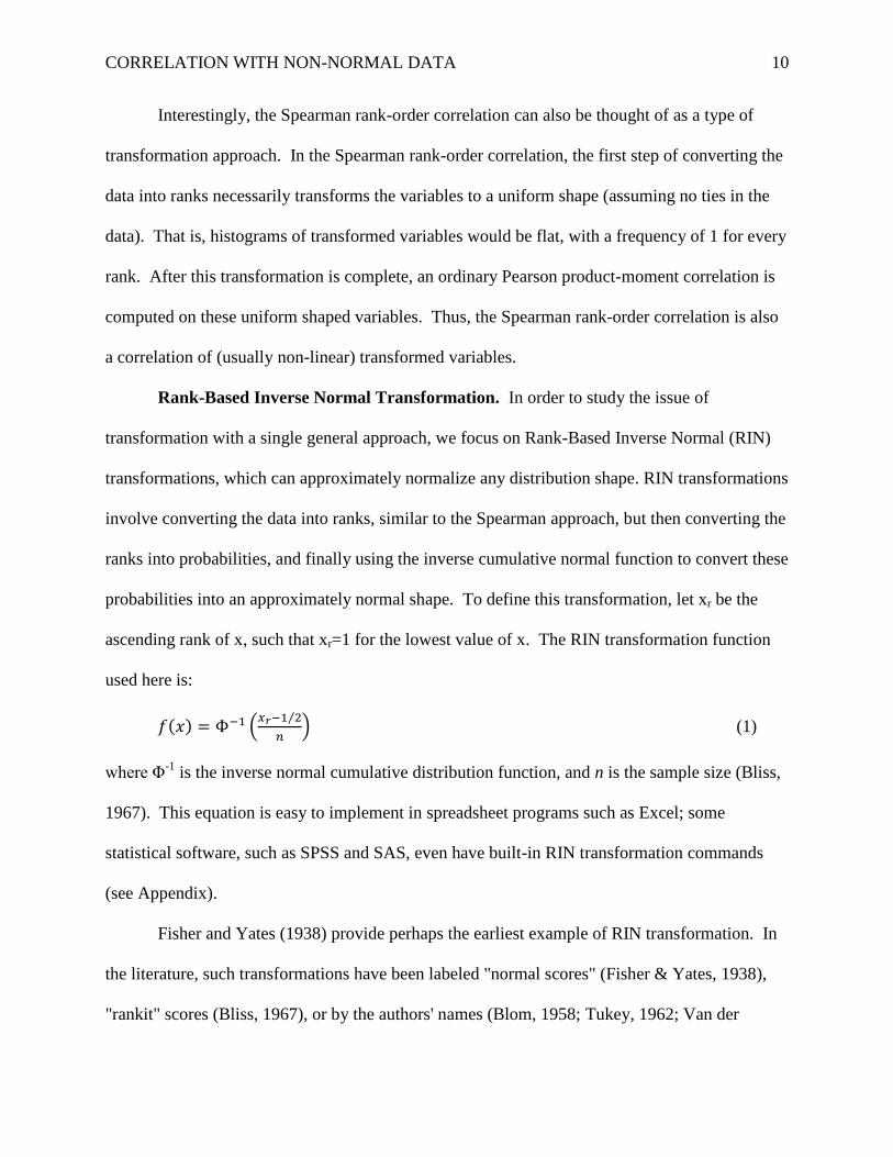
Rank-Based Inverse Normal Transformation. In order to study the issue of
transformation with a single general approach, we focus on Rank-Based Inverse Normal (RIN)
transformations, which can approximately normalize any distribution shape. RIN transformations
involve converting the data into ranks, similar to the Spearman approach, but then converting the
ranks into probabilities, and finally using the inverse cumulative normal function to convert these
probabilities into an approximately normal shape. To define this transformation, let xr be the
ascending rank of x, such that xr=1 for the lowest value of x. The RIN transformation function
used here is:
( ) ( ⁄
) (1)
where Φ-1
is the inverse normal cumulative distribution function, and n is the sample size (Bliss,
1967). This equation is easy to implement in spreadsheet programs such as Excel; some
statistical software, such as SPSS and SAS, even have built-in RIN transformation commands
(see Appendix).
Fisher and Yates (1938) provide perhaps the earliest example of RIN transformation. In
the literature, such transformations have been labeled "normal scores" (Fisher & Yates, 1938),
"rankit" scores (Bliss, 1967), or by the authors' names (Blom, 1958; Tukey, 1962; Van der
CORRELATION WITH NON-NORMAL DATA 11
Waerden, 1952). The multitude of labels is at least partly due to the multitude of equation
variations, variations which most commonly involve subtracting small constants from the
numerator and denominator of the fraction in Equation 1 (for a review, see Beasley, Erickson, &
Allison, 2009). However, these variations produce transformations that are almost perfectly
correlated with one another (all rs > .99 for the sample sizes considered in the present research),
and so it is unlikely that such variations would affect the results in the current research (Tukey,
1962; also see Beasley et al., 2009). In our simulations we use the Bliss (1967) ―rankit‖ equation
(Equation 1), and we refer to it broadly as a RIN transformation because the results are likely to
generalize to all RIN transformations (i.e., because all RIN transformations are nearly linear
transformations of one another). Bliss’s (1967) rankit equation was chosen because recent
simulation research suggests that of the rank-based normalizing equations, the rankit equation
best approximated the intended standard deviation of the transformed distribution (Solomon &
Sawilowsky, 2009).
Little is known about RIN transformation's ability to maximize power and control Type I
error rate for tests of correlations. In other tests, such as tests of equality of means, several
studies have found RIN approaches to be inferior to other non-parametric approaches, such as
Welch's test (Beasley et al., 2009; Penfield, 1994; Tomarken & Serlin, 1986). However, it is
important to note that rank-based transformations may be more effective when testing
correlations than when testing differences among means. With tests of correlations, X and Y
variables are typically assigned ranks separately from one another (for example, there is a 1st
rank for X and a 1st rank for Y). In contrast, for tests of equality of means, ranks are assigned on
the combined data, which can cause non-normal distribution shapes to linger even after the rank
transformation (Zimmerman, 2011). This problem is avoided when ranking is performed in the
CORRELATION WITH NON-NORMAL DATA 12
context of correlations, and so RIN transformation might fare better with a test of association
rather than a test of equality of means. In fact, because RIN transformation guarantees an
approximately normal distribution, it may be a useful and widely applicable transformation
approach for assessing bivariate associations.
Permutation Test of Correlation. The permutation (or randomization) test originated
with the work of Fisher (1935) and Pitman (1937), and several contemporary statistical
methodologists (e.g., Good, 2005; Mielke & Berry, 2007) recommend using permutation-based
procedures in a broad array of situations, especially with small sample sizes and non-normally
distributed variables. The permutation test involves randomly re-pairing X and Y variables so as
to create a distribution of rs expected by the Null hypothesis. Because the probability from a
permutation test is computed by comparing the obtained test statistic against the ―permutation,‖
rather than theoretical, distribution of the test statistic, many argue that normal-theory test
assumptions (e.g., random sampling from a specified population, normally distributed errors) do
not have to be met in order to draw valid inferences from a permutation test. It should be noted,
however, that in the absence of random sampling from a specified population, the permutation
test results cannot truly be generalized from the sample to the specific population (see May &
Hunter, 1993). Nevertheless, the flexibility of permutation tests and their apparent ―distribution-
free‖ nature have led many researchers to view the permutation test as a general solution to
assumption violations (Blair & Karniski, 1993; Cervone, 1985; Wampold & Worsham, 1986).
In fact, permutation tests have even been referred to as the ―gold standard‖ of hypothesis testing
(e.g., Conneely & Boehnke, 2007, p. 1158; Hesterberg, Monaghan, Moore, Clipson, & Epstein,
2003, p. 61).
CORRELATION WITH NON-NORMAL DATA 13
Comparing permutation tests of the Pearson r to simple t-tests of the Pearson r,
permutation tests do not always solve all assumption violation problems, and simulation results
on this issue have been mixed (Hayes, 1996; Keller-McNulty & Higgins, 1987; Rasmussen,
1989). When normality assumptions are violated in particular, permutation tests tend to do well
at controlling Type I error rate (Hayes, 1996). At the same time, though, permutation tests may
provide little power benefit over the simple Pearson approach in the context of non-normal data
(Good, 2009). It appears that the empirical literature is mixed regarding the relative merits of the
permutation test versus Pearson’s r. In some situations the permutation test is more robust
whereas in others the two procedures evidence similar levels of validity.
Bootstrap Tests of Correlation. The bootstrap test (Efron, 1979) is very similar to the
permutation test. However, whereas the permutation test involves resampling without
replacement, the bootstrap test involves resampling with replacement. Good (2005) provides an
accessible overview of the permutation test and bootstrap procedures. One possible advantage of
the bootstrap is that it allows a larger number of possible resampling combinations (by sampling
with replacement) than would otherwise be possible.
One kind of bootstrap test for correlation coefficients is the univariate bootstrap test (Lee
& Rodgers, 1998). Like the permutation test, the univariate bootstrap resamples X and Y
variables independently (not in pairs) so as to create a theoretical Null Hypothesis sampling
distribution. The only difference is that the univariate bootstrap resamples with replacement, so
particular values of X and/or Y might be represented more or less often in the bootstrap sampling
distribution than they were in the original sample. Simulation studies of the univariate bootstrap
test of the correlation suggest that it preserves the intended Type I error rate even with non-
CORRELATION WITH NON-NORMAL DATA 14
normal data. In terms of power, the univariate bootstrap test often provides similar or only
slightly lower power than the Pearson t-test (Lee & Rodgers, 1998).
Whereas the univariate bootstrap test of the correlation resamples X and Y
independently, the bivariate bootstrap test resamples X and Y in pairs (Lunneborg, 1985). The
resulting sampling distribution is used to create a confidence interval of the observed correlation,
and if this confidence interval does not include 0, the null hypothesis of zero correlation is
rejected. Unfortunately, numerous simulation studies of the bivariate bootstrap test of a
correlation have shown that it inflates Type I error rates, both for normal and non-normal data,
and even when various possible ―corrections‖ to the bootstrap formula are applied (Beasley et
al., 2007; Lee & Rodgers, 1998; Rasmussen, 1987; Strube, 1988). Overall, the literature
suggests that the univariate bootstrap test might provide a possible alternative to the Pearson t-
test, but the bivariate bootstrap test would not because it is too liberal at rejecting the null
hypothesis.
Summary and Implications. Generally speaking, Pearson’s r is fairly robust to non-
normality. Exceptions include markedly non-normal distributions (e.g., the highly kurtotic
distributions) where Pearson’s r demonstrates poor Type I error rate control, and increasing
sample size does not necessarily alleviate this problem. Spearman’s rank-order correlation has
also shown better Type I error rate control, as compared to Pearson's r, in some cases.
Furthermore, Spearman’s r is often more powerful than Pearson’s r in the context of non-
normality. When data are non-normal, nonlinear transformations often improve the power of
correlation tests, but little is known about the effectiveness of RIN transformation in particular.
Among resampling methods, the permutation test and univariate bootstrap tests are robust to
many types of non-normality, but may provide little if any power advantage.
CORRELATION WITH NON-NORMAL DATA 15
Simulation 1
Previous literature on correlation with non-normal data has separately compared the
Pearson product-moment correlation to alternative approaches in isolation. However, these
latter, nonparametric approaches have not been simultaneously compared to one another, and so
it is unclear as to which alternatives to the Pearson's r are optimal and under what circumstances.
Even when common statistical textbooks discuss nonparametric correlation approaches, it is hard
to find clear guidance on which one to use in practice. Additionally, to our knowledge, no
previous research has examined the Type I error and power implications of RIN transformation,
particularly when applied to the Pearson correlation. RIN transformation may be a particularly
useful transformation because it can approximate a normal distribution shape regardless of the
initial distribution's shape.
To address these issues, Monte Carlo simulation was used to compare the performance of
various correlational methods. In the first simulation, we compared twelve recommended
approaches to testing the significance of a correlation coefficient when data are non-normally
distributed: t-test of the Pearson product-moment correlation, z-test of the Fisher (1928) r-to-z
transformed Pearson correlation, t-test of the Spearman rank-order correlation, "exact" test of the
Spearman rank-order correlation, four different nonlinear transformations of the marginal X and
Y distributions prior to performing a t-test on the correlation (i.e., the Box-Cox, Yeo-Johnson,
arcsine, and RIN transformations), and four different resampling-based procedures (the
permutation test, univariate Bootstrap test, bivariate Bootstrap test, and the bivariate Bootstrap
test with Bias Correction and Acceleration). The second simulation further examined the relative
power of select procedures from Simulation 1 in the context of extremely large effect sizes.
Simulation 2 is presented following the Results and Discussion of Simulation 1.
CORRELATION WITH NON-NORMAL DATA 16
For the purpose of generality, we examined 6 different marginal distribution shapes (i.e.,
the shape that would appear when examining a simple histogram of one variable). The
distributions were selected to represent the range of distributional shapes that often occur in
psychological data: Normal, Weibull, Chi-squared, uniform, bimodal, and long-tailed. These
distributions are depicted in Figure 1. Although these distributions are representative of the
kinds of distributions that occur in psychological research, the list is by no means exhaustive.
Our goal was not to examine all distributions (an unrealistic goal), but rather to sample the range
of distributions that often occur in psychological research.
The primary goal of Simulation 1 was to determine which methods preserved the
intended Type I error rate while maximizing power, and under what conditions they did so. To
examine these issues, analysis focused on the most common nominal alpha used in psychological
research, alpha=.05. To anticipate, among the more robust measures, some methods produced
greater power than others, and sometimes in ways that were surprising given common textbook
recommendations.
Method
We examined the probability that a 2-tailed test would be significant with a null
hypothesis of ρ = 0 and an alpha set at .05. Additionally, we recorded the probability that the
rejection was in the correct (i.e., positive) tail region. The 12 methods of testing the significance
of a correlation were compared across 11 combinations of distribution shapes, 6 sample sizes,
and 3 effect sizes (ρ = 0, .1, and .5). For each combination of distribution shape, sample size,
and effect size, 10,000 simulations were conducted. 10,000 simulations makes the 95%
confidence interval of the proportion +/- .010, at most. Within each simulation, the resampling
approaches (e.g. permutation test) used 9,999 resamples each. This number was chosen such that
CORRELATION WITH NON-NORMAL DATA 17
the quantity of the number of resamples plus 1, when multiplied by alpha, would result in an
integer (in this case, 500). This is a desirable property of the number of resamples because it
creates clear-cut bins for the rejection region (Beasley & Rodgers, 2009). Simulations were
conducted using the open-source software package, R (R Development Core Team, 2010). The
code is freely available on request, and parts of the code were based on previously published
code (Good, 2009; Ruscio & Kaczetow, 2008).
12 Tests of the Significance of a Correlation
1. Pearson - t-test. The traditional t-test of the Pearson product-moment correlation was
conducted.
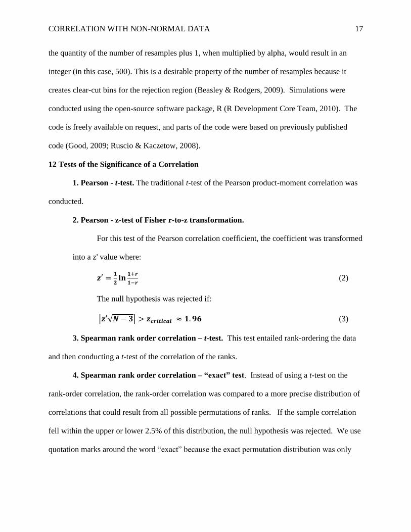
2. Pearson - z-test of Fisher r-to-z transformation.
For this test of the Pearson correlation coefficient, the coefficient was transformed
into a z' value where:
(2)
The null hypothesis was rejected if:
| √ | (3)
3. Spearman rank order correlation – t-test. This test entailed rank-ordering the data
and then conducting a t-test of the correlation of the ranks.
4. Spearman rank order correlation – “exact” test. Instead of using a t-test on the
rank-order correlation, the rank-order correlation was compared to a more precise distribution of
correlations that could result from all possible permutations of ranks. If the sample correlation
fell within the upper or lower 2.5% of this distribution, the null hypothesis was rejected. We use
quotation marks around the word ―exact‖ because the exact permutation distribution was only
CORRELATION WITH NON-NORMAL DATA 18
computed for n = 5. For all other n’s, the permutation distribution was estimated by an
Edgeworth series approximation (Best & Roberts, 1975).
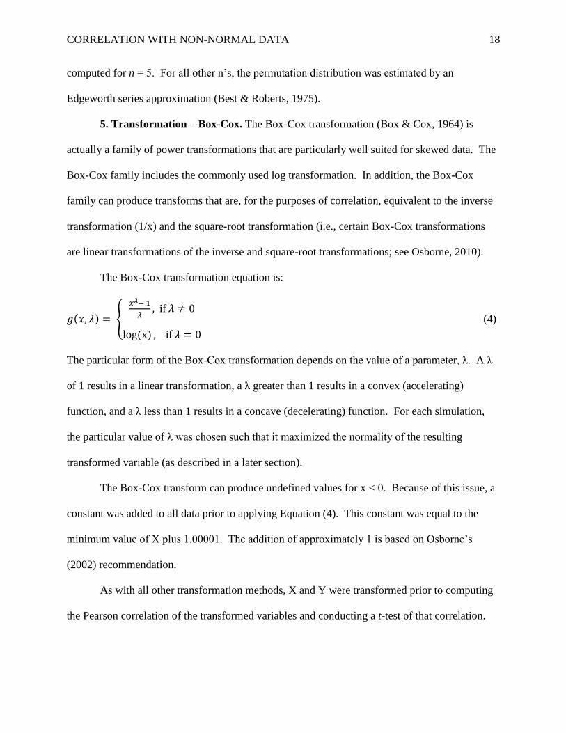
5. Transformation – Box-Cox. The Box-Cox transformation (Box & Cox, 1964) is
actually a family of power transformations that are particularly well suited for skewed data. The
Box-Cox family includes the commonly used log transformation. In addition, the Box-Cox
family can produce transforms that are, for the purposes of correlation, equivalent to the inverse
transformation (1/x) and the square-root transformation (i.e., certain Box-Cox transformations
are linear transformations of the inverse and square-root transformations; see Osborne, 2010).
The Box-Cox transformation equation is:
( ) {
( )
(4)
The particular form of the Box-Cox transformation depends on the value of a parameter, λ. A λ
of 1 results in a linear transformation, a λ greater than 1 results in a convex (accelerating)
function, and a λ less than 1 results in a concave (decelerating) function. For each simulation,
the particular value of λ was chosen such that it maximized the normality of the resulting
transformed variable (as described in a later section).
The Box-Cox transform can produce undefined values for x < 0. Because of this issue, a
constant was added to all data prior to applying Equation (4). This constant was equal to the
minimum value of X plus 1.00001. The addition of approximately 1 is based on Osborne’s
(2002) recommendation.
As with all other transformation methods, X and Y were transformed prior to computing
the Pearson correlation of the transformed variables and conducting a t-test of that correlation.
CORRELATION WITH NON-NORMAL DATA 19
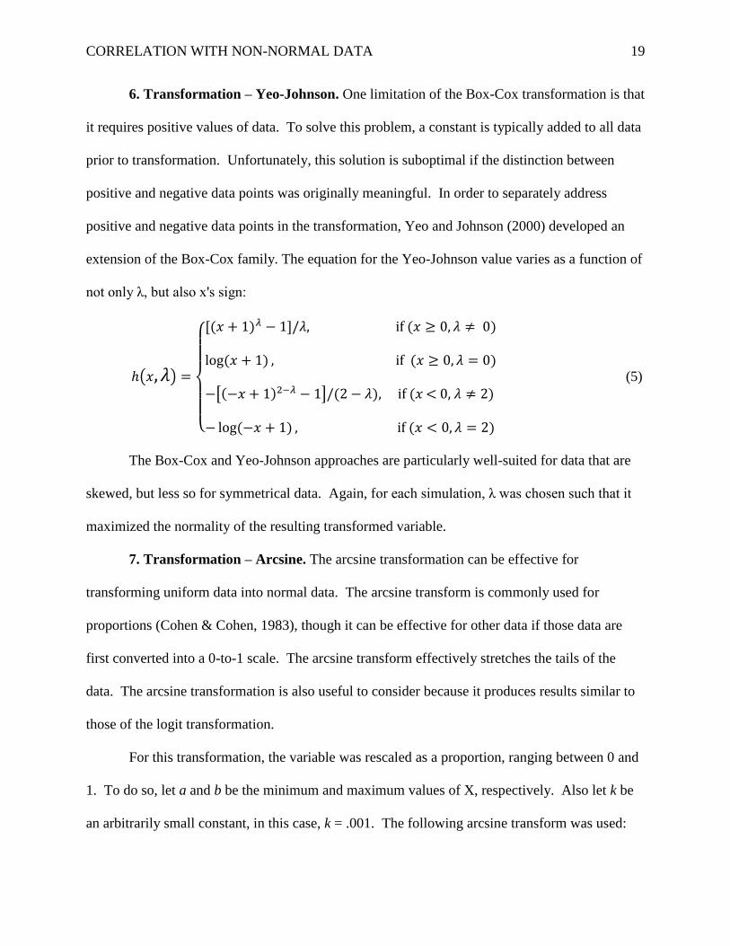
6. Transformation – Yeo-Johnson. One limitation of the Box-Cox transformation is that
it requires positive values of data. To solve this problem, a constant is typically added to all data
prior to transformation. Unfortunately, this solution is suboptimal if the distinction between
positive and negative data points was originally meaningful. In order to separately address
positive and negative data points in the transformation, Yeo and Johnson (2000) developed an
extension of the Box-Cox family. The equation for the Yeo-Johnson value varies as a function of
not only λ, but also x's sign:
( )
{
( ) ( )
( ) ( )
[( ) ] ( ) ( )
( ) ( )
(5)
The Box-Cox and Yeo-Johnson approaches are particularly well-suited for data that are
skewed, but less so for symmetrical data. Again, for each simulation, λ was chosen such that it
maximized the normality of the resulting transformed variable.
7. Transformation – Arcsine. The arcsine transformation can be effective for
transforming uniform data into normal data. The arcsine transform is commonly used for
proportions (Cohen & Cohen, 1983), though it can be effective for other data if those data are
first converted into a 0-to-1 scale. The arcsine transform effectively stretches the tails of the
data. The arcsine transformation is also useful to consider because it produces results similar to
those of the logit transformation.
For this transformation, the variable was rescaled as a proportion, ranging between 0 and
1. To do so, let a and b be the minimum and maximum values of X, respectively. Also let k be
an arbitrarily small constant, in this case, k = .001. The following arcsine transform was used:
CORRELATION WITH NON-NORMAL DATA 20
( ) √( ) ( ) (6)
8. Transformation – RIN. Data were transformed via Equation 1 prior to conducting a t-
test of the Pearson correlation of the transformed data.
9. Resampling – Permutation test. For the permutation test, a permutation distribution
was generated by randomly re-assigning values of the X variable (this effectively re-paired both
X and Y) and saving the resulting Pearson correlation for each such permutation. This procedure
was repeated in order to form a permutation sampling distribution of correlations expected under
the null hypothesis. If the sample Pearson r was outside of the 2.5th
to 97.5th
percentile of this
permutation sampling distribution, the Null hypothesis was rejected.
10. Resampling – Univariate Bootstrap Test. The univariate bootstrap test was
identical to the permutation test except that X and Y were both sampled with replacement in
order to form the resampling distribution. Sampling of X and Y was independent (they were
unpaired). In situations when the bootstrap sample of X or bootstrap sample of Y consisted
entirely of the same number, the bootstrap correlation was undefined, and so the bootstrap
sample was discarded and replaced by another bootstrap sample (see Strube, 1988). For
example, if the original sample was X={1.2, 0.5, -1.7, 3.2, -0.8}, and an initial bootstrap sample
consisted of X={1.2, 1.2, 1.2, 1.2, 1.2}, then that bootstrap sample would be replaced.
11. Resampling – Bivariate Bootstrap Test. In the bivariate bootstrap test, yoked pairs
of data (X and Y) were sampled with replacement, and the Pearson correlation was saved for
each such bootstrap sample. Undefined bootstrap sample correlations were handled in the same
way as explained above. This procedure was repeated in order to generate a bootstrap sampling
distribution of correlations for the observed correlation. If the 2.5th to 97.5th percentile of this
CORRELATION WITH NON-NORMAL DATA 21
bootstrap sampling distribution did not include 0, the Null hypothesis was rejected. Thus, this
constituted a bivariate "percentile" bootstrap test.
12. Resampling – Bivariate Bootstrap with Bias Correction and Acceleration (BCa)
Test. This test was identical to the above-mentioned bivariate bootstrap, except that the 95%
confidence interval was constructed through the BCa approach (Efron & Tibshirani, 1993, pp.
184-188). This approach shifts and widens the bounds of the 95%
confidence interval so as to
make the interval more accurate, with the errors in intended coverage approaching 0 more
quickly as n increases, at least as compared to the bivariate percentile bootstrap (method 11). A
description of the Efron and Tibshirani BCa approach can be found online (Beasley et al., 2007,
supplementary materials).
Selecting λ Parameter for Transformations
For the Box-Cox and Yeo-Johnson transformations, values of λ were sought that
maximized the normality of the resulting transformed variable. Specifically, λ was optimized
such that it maximized the correlation of the coordinates of the normal qq-plot of the variable.
The normal qq-plot is a plot of the quantiles of the observed data against the quantiles expected
by a normal distribution. Because the normal qq-plot will tend to be more linear as the observed
data is more normal, higher correlations indicate more normal shapes (Filliben, 1975). This one-
dimensional optimization was performed with R’s ―optimize‖ function (R Development Core
Team, 2010). This optimization function seeks to converge on the best λ by iteratively using test
values of λ, with the test values of λ chosen by a combination of a rapid algorithm that assumes a
polynomial function (successive parabolic interpolation) and a slower but more robust algorithm
(golden section search). The search had the constraint: -5 < λ < 5. This range was chosen
because, in pilot simulations, larger ranges for λ provided no reliable benefit to the resulting
CORRELATION WITH NON-NORMAL DATA 22
normal qq-plot correlations. Optimization was done separately for each simulation, applying
each of the two methods to both X and Y. Optimization was blind to the underlying population
distribution shape. Note that the optimization was done independently for X and Y, and so the
optimization could not capitalize on chance to inflate the resulting association between the two
variables.
Distribution Shapes
In terms of the distribution shapes, a Weibull distribution was used to simulate slightly
skewed data, a common shape in many psychological datasets. The Weibull distribution is also
relevant because it resembles the distribution of reaction times in a variety of tasks, including not
only simple tasks like reading, but also more complicated tasks involving the learning of
mathematical functions (Berry, 1981; Logan, 1992). For the present simulations, the Weibull
distribution had shape=1.5 and scale=1. These parameters are in the range of parameters
common to human task performance times, and these parameters produce a slight but noticeable
skew (see Figure 1). The Chi2 distribution was chosen to provide an even more skewed shape. In
particular, the Chi2 with 1 degree of freedom was used. This distribution represents roughly the
most extreme skewness and kurtosis typically found in psychological data (Beasley et al., 2007;
Micceri, 1989). The uniform distribution ranged from 0 to 1 (the range was arbitrary because all
distributions were standardized in a later step). The bimodal distribution was a mixture of two
normal distributions with different population means but the same standard deviation. The
means were separated by 5 standard deviations so as to make the bimodality noticeable via visual
inspection of a histogram. In contrast, the long-tailed distribution was a mixture of two normal
distributions with the same mean but different standard deviations. In order to create extremely
long tails and high kurtosis, this distribution was created by sampling with a .9 chance from a
CORRELATION WITH NON-NORMAL DATA 23
normal with a small standard deviation, and sampling with a .1 probability from a normal with a
standard deviation 10 times as large. All population distribution equations were rescaled so that
the population mean was 0 and population standard deviation was 1. Other descriptive statistics,
including skewness and excess kurtosis, are summarized in Table 1. We examined situations
where X and Y were both the same distribution shape and also where X was normal but Y was
not. This created a total of 11 combinations of distribution shapes.
Sample and Effect Sizes
The six sample sizes were N=5, 10, 20, 40, 80, and 160. A ρ of 0 was used for the null
hypothesis of zero correlation, .1 was used for a small effect size, and .5 for a large effect size
(Cohen, 1977). Thus, a large range of both sample and effect sizes could be compared. Though
the simulations did not include a medium effect size (ρ=.3), to anticipate, the relative
performance of various significance tests was not qualitatively altered by the effect size.
Generating Correlated Non-normal Data
In order to simulate the specified correlated non-normal data, we used an iterative
algorithm developed by Ruscio and Kaczetow (2008). In this procedure, X0 and Y0 are
generated with the desired non-normal distribution shapes (e.g., bimodal), but they are generated
independently of one another. X1 and Y1 are generated such that they are bivariate normal with a
nonzero intermediate correlation coefficient. The first intermediate correlation value tried is the
target correlation value. X0 and Y0 are used to replace X1 and Y1, and they are replaced in such a
way that the rank-orders of corresponding variables are preserved. However, because the
variables are no longer both normal, their observed correlation may be deflated or inflated
relative to the target correlation. A new intermediate correlation is chosen - adjusted to be either
higher or lower than the original intermediate correlation - based on the difference between the
CORRELATION WITH NON-NORMAL DATA 24
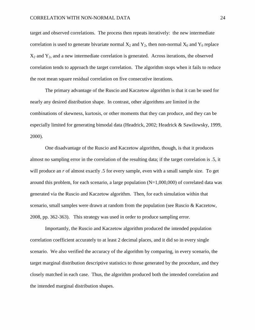
target and observed correlations. The process then repeats iteratively: the new intermediate
correlation is used to generate bivariate normal X2 and Y2, then non-normal X0 and Y0 replace
X2 and Y2, and a new intermediate correlation is generated. Across iterations, the observed
correlation tends to approach the target correlation. The algorithm stops when it fails to reduce
the root mean square residual correlation on five consecutive iterations.
The primary advantage of the Ruscio and Kaczetow algorithm is that it can be used for
nearly any desired distribution shape. In contrast, other algorithms are limited in the
combinations of skewness, kurtosis, or other moments that they can produce, and they can be
especially limited for generating bimodal data (Headrick, 2002; Headrick & Sawilowsky, 1999,
2000).
One disadvantage of the Ruscio and Kaczetow algorithm, though, is that it produces
almost no sampling error in the correlation of the resulting data; if the target correlation is .5, it
will produce an r of almost exactly .5 for every sample, even with a small sample size. To get
around this problem, for each scenario, a large population (N=1,000,000) of correlated data was
generated via the Ruscio and Kaczetow algorithm. Then, for each simulation within that
scenario, small samples were drawn at random from the population (see Ruscio & Kaczetow,
2008, pp. 362-363). This strategy was used in order to produce sampling error.
Importantly, the Ruscio and Kaczetow algorithm produced the intended population
correlation coefficient accurately to at least 2 decimal places, and it did so in every single
scenario. We also verified the accuracy of the algorithm by comparing, in every scenario, the
target marginal distribution descriptive statistics to those generated by the procedure, and they
closely matched in each case. Thus, the algorithm produced both the intended correlation and
the intended marginal distribution shapes.
CORRELATION WITH NON-NORMAL DATA 25
Results and Discussion
Type I Error
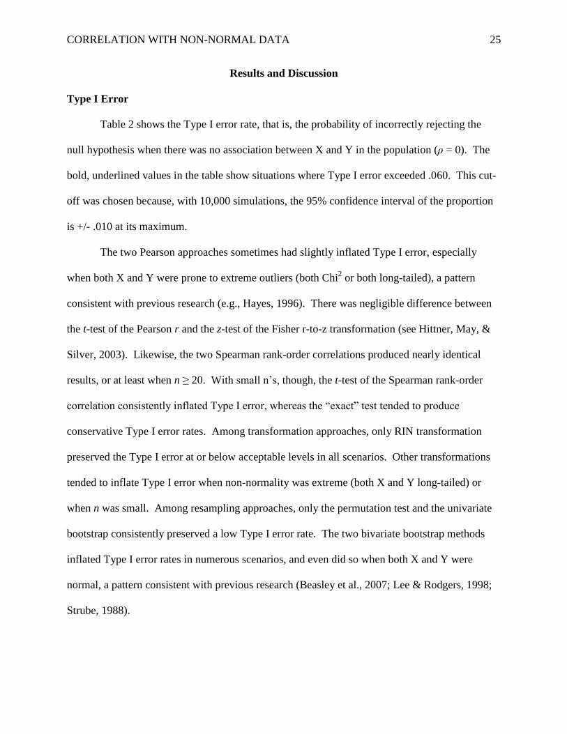
Table 2 shows the Type I error rate, that is, the probability of incorrectly rejecting the
null hypothesis when there was no association between X and Y in the population (ρ = 0). The
bold, underlined values in the table show situations where Type I error exceeded .060. This cut-
off was chosen because, with 10,000 simulations, the 95% confidence interval of the proportion
is +/- .010 at its maximum.
The two Pearson approaches sometimes had slightly inflated Type I error, especially
when both X and Y were prone to extreme outliers (both Chi2 or both long-tailed), a pattern
consistent with previous research (e.g., Hayes, 1996). There was negligible difference between
the t-test of the Pearson r and the z-test of the Fisher r-to-z transformation (see Hittner, May, &
Silver, 2003). Likewise, the two Spearman rank-order correlations produced nearly identical
results, or at least when n ≥ 20. With small n’s, though, the t-test of the Spearman rank-order
correlation consistently inflated Type I error, whereas the ―exact‖ test tended to produce
conservative Type I error rates. Among transformation approaches, only RIN transformation
preserved the Type I error at or below acceptable levels in all scenarios. Other transformations
tended to inflate Type I error when non-normality was extreme (both X and Y long-tailed) or
when n was small. Among resampling approaches, only the permutation test and the univariate
bootstrap consistently preserved a low Type I error rate. The two bivariate bootstrap methods
inflated Type I error rates in numerous scenarios, and even did so when both X and Y were
normal, a pattern consistent with previous research (Beasley et al., 2007; Lee & Rodgers, 1998;
Strube, 1988).

CORRELATION WITH NON-NORMAL DATA 26
Overall, only 4 methods consistently preserved the Type I error rate at or below the
intended alpha in all scenarios: Spearman ―exact‖ test, RIN transformation, permutation test, and
univariate bootstrap test. We refer to these 4 methods as alpha-robust methods. Other
approaches tended to inflate Type I error above the nominal alpha, particularly when n was small
or when X and Y were especially prone to outliers on one or both tails (i.e., Chi2 or Long-
Tailed).
Statistical Power
As summarized in Figure 2, when at least one variable was non-normal, there were power
differences among the alpha-robust measures and the Pearson t-test of the correlation. In
particular, for moderate to large sample sizes (N ≥ 20), RIN transformation tended to produce
higher or at least similar power as compared to other approaches. As described in more detail
below, power was also a function of the type of the particular shapes of X and Y.
Small Effect Size. Table 3 shows the power with a small effect size, that is, the
probability of correctly rejecting the null hypothesis when ρ = .1. Note that, even though the
Pearson correlation was .1, the underlying strength of the monotonic association between X and
Y may vary based on the distribution shapes. Of course, all distribution combinations in the
table had some non-zero population effect, and so higher values in the table indicate greater
power, a desirable property. Because of the number of simulations, the largest 95% confidence
interval of the mean in Table 3 was ± .010.
When both X and Y were normal (Table 3, upper-most panel), most methods showed
similar levels of power in most scenarios. Of course, the bivariate bootstrap methods did show
higher power than other approaches, but the bivariate bootstrap methods also inflated Type I
errors.
CORRELATION WITH NON-NORMAL DATA 27
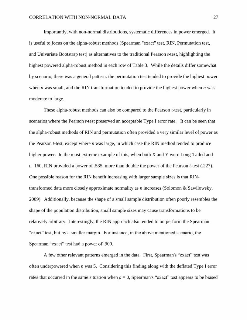
Importantly, with non-normal distributions, systematic differences in power emerged. It
is useful to focus on the alpha-robust methods (Spearman "exact" test, RIN, Permutation test,
and Univariate Bootstrap test) as alternatives to the traditional Pearson t-test, highlighting the
highest powered alpha-robust method in each row of Table 3. While the details differ somewhat
by scenario, there was a general pattern: the permutation test tended to provide the highest power
when n was small, and the RIN transformation tended to provide the highest power when n was
moderate to large.
These alpha-robust methods can also be compared to the Pearson t-test, particularly in
scenarios where the Pearson t-test preserved an acceptable Type I error rate. It can be seen that
the alpha-robust methods of RIN and permutation often provided a very similar level of power as
the Pearson t-test, except where n was large, in which case the RIN method tended to produce
higher power. In the most extreme example of this, when both X and Y were Long-Tailed and
n=160, RIN provided a power of .535, more than double the power of the Pearson t-test (.227).
One possible reason for the RIN benefit increasing with larger sample sizes is that RIN-
transformed data more closely approximate normality as n increases (Solomon & Sawilowsky,
2009). Additionally, because the shape of a small sample distribution often poorly resembles the
shape of the population distribution, small sample sizes may cause transformations to be
relatively arbitrary. Interestingly, the RIN approach also tended to outperform the Spearman
―exact‖ test, but by a smaller margin. For instance, in the above mentioned scenario, the
Spearman ―exact‖ test had a power of .500.
A few other relevant patterns emerged in the data. First, Spearman's ―exact‖ test was
often underpowered when n was 5. Considering this finding along with the deflated Type I error
rates that occurred in the same situation when ρ = 0, Spearman's ―exact‖ test appears to be biased
CORRELATION WITH NON-NORMAL DATA 28
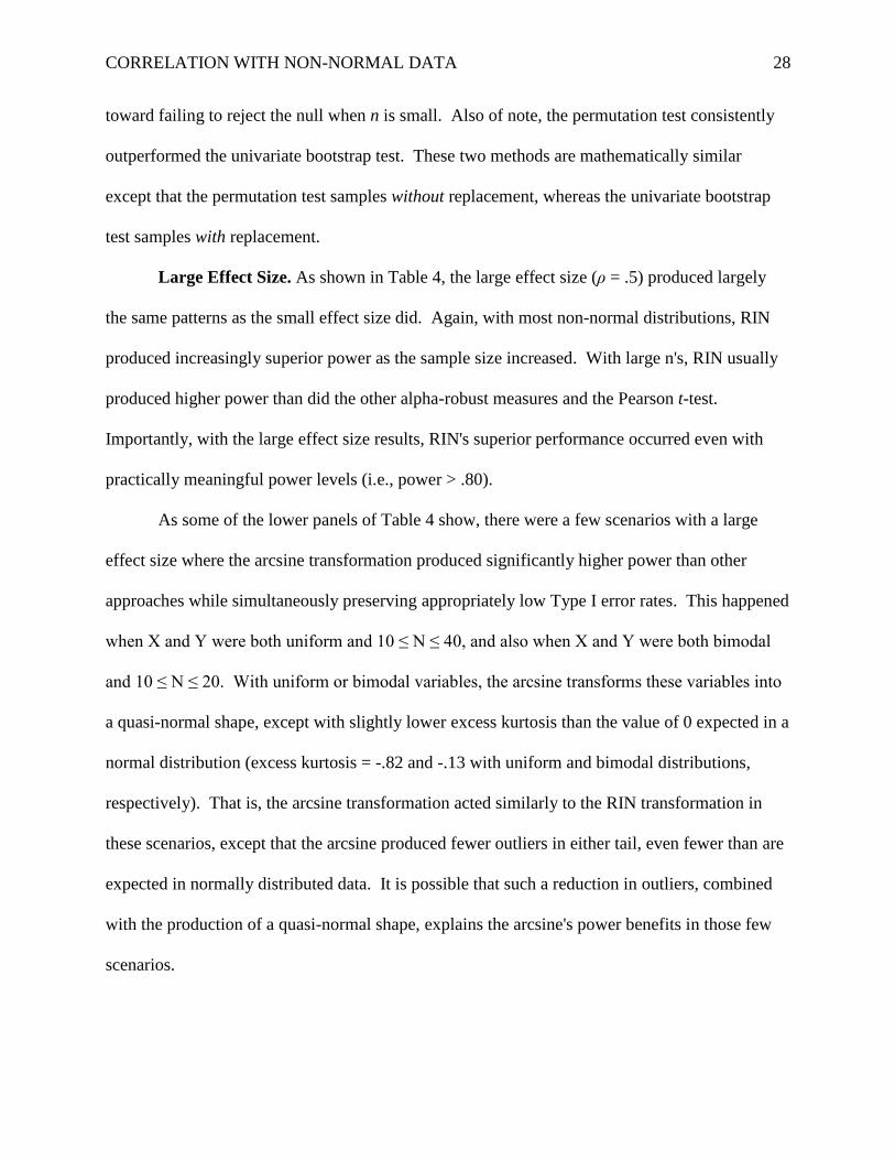
toward failing to reject the null when n is small. Also of note, the permutation test consistently
outperformed the univariate bootstrap test. These two methods are mathematically similar
except that the permutation test samples without replacement, whereas the univariate bootstrap
test samples with replacement.
Large Effect Size. As shown in Table 4, the large effect size (ρ = .5) produced largely
the same patterns as the small effect size did. Again, with most non-normal distributions, RIN
produced increasingly superior power as the sample size increased. With large n's, RIN usually
produced higher power than did the other alpha-robust measures and the Pearson t-test.
Importantly, with the large effect size results, RIN's superior performance occurred even with
practically meaningful power levels (i.e., power > .80).
As some of the lower panels of Table 4 show, there were a few scenarios with a large
effect size where the arcsine transformation produced significantly higher power than other
approaches while simultaneously preserving appropriately low Type I error rates. This happened
when X and Y were both uniform and 10 ≤ N ≤ 40, and also when X and Y were both bimodal
and 10 ≤ N ≤ 20. With uniform or bimodal variables, the arcsine transforms these variables into
a quasi-normal shape, except with slightly lower excess kurtosis than the value of 0 expected in a
normal distribution (excess kurtosis = -.82 and -.13 with uniform and bimodal distributions,
respectively). That is, the arcsine transformation acted similarly to the RIN transformation in
these scenarios, except that the arcsine produced fewer outliers in either tail, even fewer than are
expected in normally distributed data. It is possible that such a reduction in outliers, combined
with the production of a quasi-normal shape, explains the arcsine's power benefits in those few
scenarios.
CORRELATION WITH NON-NORMAL DATA 29
With small sample sizes, the permutation test was often more powerful than the other
alpha-robust approaches. The permutation test usually provided similar or higher power than the
Pearson correlation with small n's, so long as the distributions were especially non-normal. The
permutation test’s success in such scenarios may be due to that fact that the test does not require
a specified distribution shape, normal or otherwise. One limitation of these results is that,
because the sample sizes were small when the permutation test performed well, the situations
where it performed well tended to have low absolute levels of power. This limitation was
addressed in Simulation 2.
Did the RIN Transformation or Permutation Methods Reject the Null Hypothesis at
the Correct Tail? Non-normal data may have a deflated Pearson correlation coefficient, one
that underestimates the underlying monotonic association between the variables (Calkins, 1974;
Dunlap, Burke, & Greer, 1995; Lancaster, 1957). Because of this, nonlinear transforms toward
normality, such as RIN, may produce a larger correlation coefficient than that of the
untransformed data. This notion is consistent with Tables 3 and 4, which show that power can
be much larger for the non-normal data that was transformed toward normality than for the
normal data that was not.
More generally, the correlation coefficient derived from alternative methods is not
expected to be equal to the Pearson correlation coefficient of the untransformed data. Thus, it is
unclear as to what exact numerical baseline the alternative correlation coefficients should be
compared to in order to gauge their bias. At the very least, these alternatives should preserve the
sign of the correlation, and avoid rejecting the Null hypothesis based on the wrong tail of the
distribution. Overall, for non-zero effect sizes, the probability of rejecting the Null hypothesis at
the wrong (left) tail was very low, and it was similar for the traditional Pearson t test, the RIN
CORRELATION WITH NON-NORMAL DATA 30
transformation, and permutation test (.004 for each). Thus, the power differences among
methods cannot be accounted for simply by some methods rejecting the wrong tail of the
distribution.
Simulation 2
Simulation 1 revealed advantages of the permutation test with small sample sizes (and
non-normal data). However, for these sample sizes, the power was much lower in these
scenarios than the power levels that researchers typically seek (e.g., power > .80). To determine
whether the permutation test provided high power even at more desirable absolute levels of
power, a small follow-up simulation was conducted. Simulation 2 used an extremely large effect
size (ρ = .8) and small sample sizes. Simulation 2 focused on the alpha-robust methods, that is,
the four methods that did not inflate the Type I error rate. In addition, Simulation 2 also
examined the Pearson t-test as a basis for comparison. The primary goal was to examine which
of these alpha-robust procedures could attain practically meaningful levels of power with very
small sample sizes, and the conditions under which they could do so.
Method
Simulation 2 was nearly identical to Simulation 1. However, ρ was set to .8.
Additionally, only n’s of 5 and 10 were examined because larger sample sizes produced ceiling
effects because of the extremely large effect size. Finally, five methods were considered:
Pearson t-test, Spearman ―exact‖ test, RIN transformation, Permutation test, and Univariate
Bootstrap test.
Results and Discussion
As shown in Table 5, the results suggest that the benefits of the permutation test often
generalize to situations with practically meaningful power. Among alpha-robust methods, the
CORRELATION WITH NON-NORMAL DATA 31
permutation test always provided the highest power when n was 5, and it often did so when n
was 10. When the permutation test’s power was surpassed by another alpha-robust method, it
was always the RIN method, and only when n was 10 and both variables were extremely non-
normal. As before, the permutation test showed consistently higher power than its ―sampling-
with-replacement‖ counterpart, the univariate bootstrap test.
These extremely large effect size results again emphasize the value of the permutation
test when n is small and data are non-normal. However, it should be noted that the permutation
test was sometimes inferior to the Pearson t-test, especially when the data were only slightly non-
normal. For example, when data were only slightly skewed (one or both variables were
Weibull), the Pearson t-test often provided higher power than the permutation test. In other
words, the Pearson t-test was able to withstand minor deviations from normality (Fowler, 1987).
Because the normality deviations were so minor, the benefit of making parametric assumptions
might have outweighed the cost of violation of those assumptions. Consistent with this notion,
larger violations of normality were less favorable to the Pearson approach. For example, when
data were extremely non-normal (Chi2, Bimodal, or Long-Tailed distributions), the permutation
test often outperformed the Pearson correlation in terms of power, or as shown in Simulation 1,
Type I error rate control.
General Discussion
Consistent with previous work, Pearson’s r was relatively robust to non-normality with
respect to Type I error rate, except for especially small sample sizes or especially non-normal
distribution shapes. However, other methods had even more robust Type I error control.
Specifically, the Spearman "exact" test, RIN transformation, permutation test, and univariate
bootstrap test all maintained the intended Type I error rate in all scenarios. These alpha-robust
CORRELATION WITH NON-NORMAL DATA 32
methods often produced similar or higher power than the Pearson t-test, particularly for
distributions that were extremely non-normal. With small samples, usually n ≤ 10, the
permutation test often provided a robust alternative, one with equal or greater power than the
Pearson t-test (Simulations 1 and 2); the permutation test also produced absolute power levels
that were large enough to be practically meaningful (Simulation 2). The permutation test’s
robustness may be due to the fact that the test does not require a specific (i.e., normal)
distribution shape. With larger samples sizes, usually n ≥ 20, the power benefits of the RIN
method became apparent (Simulation 1). These power benefits also occurred at practically
meaningful absolute levels of power (Simulation 1). In at least one case, RIN's power even
exceeded twice that of the Pearson t-test. The benefits of RIN transformation at large but not
small sample sizes may be due to limitations of transformation approaches when samples sizes
are small. With a small n, RIN-transformed data distributions may poorly approximate
normality (Solomon & Sawilowsky, 2009). More generally, with a small sample size, any
transformation is likely to be somewhat arbitrary because small samples may poorly resemble
the shapes of the populations from which they were drawn.
For both Type I error rates and power, the kind of non-normality mattered. Non-
normality was most problematic for the Pearson t-test when one or more distributions had highly
kurtotic shapes, such as the Chi2 or Long-tailed distributions (note that this pattern cannot be
explained via the variance because the population variance was equated for all distribution
shapes). These Chi2 and Long-tailed distributions were particularly prone to Type I error
inflation. This pattern converges with results from several previous Monte Carlo studies, which
have noted Type I error inflation specifically with both the Chi2 distribution and the Cauchy
distribution (another extremely kurtotic distribution; Beasley et al., 2007; Edgell & Noon, 1984;
CORRELATION WITH NON-NORMAL DATA 33
Hayes, 1996). In our simulations, the Pearson t-test with highly kurtotic distributions not only
resulted in inflated Type I errors, it also resulted in relatively low power, at least compared to the
power that could be achieved by alternative methods. For instance, when both distributions were
highly kurtotic, the power advantage of RIN over the Pearson t-test was especially noticeable.
These patterns suggest that researchers should consider using robust alternatives to the Pearson t-
test especially when distributions are highly kurtotic, and thus especially prone to outliers on one
or both tails.
Our simulations also examined the Spearman rank-order correlation, a commonly
recommended alternative to the Pearson correlation when assumptions are violated. For the
Spearman rank-order correlation with small samples (n ≤ 10), an "exact" test better maintained
the Type I error rate than the t-test, but with large samples they produced nearly identical results.
The Spearman rank-order correlation sometimes produced a noticeable power improvement
relative to the Pearson t-test, especially with large sample sizes (consistent with Zimmerman &
Zumbo, 1993). However, even then, power was still higher for the RIN transformation of the
data. This pattern of results poses a problem for many statistics textbooks which recommend the
use of nonparametric tests, including the Spearman correlation, when normal-theory assumptions
are violated and sample size is small. In the current research, the non-Pearson approaches were
most beneficial when N was large, not small. Textbooks may have encouraged nonparametric
procedures with a small N because textbooks often focused on nonparametric tests for equality of
means (e.g., the Mann-Whitney U-test). Comparatively less space has been devoted to
nonparametric tests of association.
Interestingly and in similar fashion to Pearson’s r, the permutation test was, in many
cases, less powerful than RIN transformation. The permutation test’s advantage was primarily
CORRELATION WITH NON-NORMAL DATA 34
limited to small sample size scenarios. This finding, along with the findings of others (e.g.,
Hayes, 1996), contradicts the idea that permutation tests are the ―gold standards‖ of hypothesis
testing, at least for correlations. However, the permutation test did provide a consistent power
advantage relative to the corresponding univariate bootstrap test. To our knowledge, this finding
is novel. Sampling with replacement (as in the univariate bootstrap) is sometimes thought
beneficial because it allows for more possible combinations of X and Y to create a sampling
distribution, especially when the sample size is small. However, the benefit of these additional
combinations must be offset by some other cost. One such cost could be the possibility of
repeated sampling of outliers. Such repeated sampling of outliers could expand the confidence
interval for the Null bootstrap sampling distribution, which would in turn make it more difficult
to reject the Null Hypothesis.
The current results, which favor the RIN transformation in many scenarios, may be seen
as hard to resolve with previous work that questioned the utility of the RIN approach. Most
recently, Beasley and colleagues (2009) showed that RIN transformation can, in some situations,
actually increase Type I error and reduce power. However, their simulations focused on tests of
equality of means and frequencies, not tests of the population correlation coefficient. One reason
that RIN might be more successful with correlations is that, in the rank transformation of
correlational data, the X and Y variables are ranked separately rather than together as pairs. The
separate rankings can prevent preservation of the original non-normal distribution shape
properties, a problem that can occur with other rank-based tests, such as tests of the equality of
means (see Zimmerman, 2011).
The central motivation behind the use of RIN (and other transformations) is that non-
normality can mask the underlying monotonic relationship among variables (Calkins, 1974;
CORRELATION WITH NON-NORMAL DATA 35
Dunlap, Burke, & Greer, 1995; Lancaster, 1957). Transformation toward approximate normality
allows the assumptions of the t-test of the Pearson correlation to be met, thus increasing the
likelihood that a relationship will be detected when present. Detection of this underlying
relationship via transformed variables in no way precludes additional analysis on the original,
untransformed variables. To the contrary, a significant result from a RIN transformation could
even be used to support additional testing of the data through non-linear regression or other
techniques. The significant effect provides some protection against capitalization on chance by
assuring that there is a relationship among variables before engaging in more fine-grained tests
of the nature of that relationship.
Limitations
The current simulations focused on variables from continuous distributions, but it is
unclear how well the results would generalize if variables were drawn from discrete
distributions, which can often produce ties. Additional research would be required to determine
how well the above compared approaches fare in addition to approaches specifically developed
for data with frequent ties (e.g., Goodman-Kruskal Gamma, Kendall’s tau).
Even when using continuous data, caution should be urged when using RIN
transformation with analyses that are more complicated than bivariate correlation. The RIN
transformation may produce inconsistent Type I error rates for more complicated regression
models, particularly for interaction terms (see Blair, Sawilowsky, & Higgins, 1987; Wang &
Huang, 2002). More generally, although the current results suggest that RIN transformation can
address the issue of non-normality, there is no guarantee that it can address other assumption
violations, such as heteroscedasticity, when testing the significance of correlations (see Hayes,
1996). When heteroscedasticity or factorial designs are present, rank-based methods in general
CORRELATION WITH NON-NORMAL DATA 36
often demonstrate inferior performance (Beasley et al., 2009; Salter & Fawcett, 1993;
Zimmerman, 1996). Clearly, additional research would be needed to explore the costs and
benefits of RIN in other scenarios.
The present work addresses significance testing, but not parameter estimation. For the
RIN approach, researchers might be interested in the correlation coefficient of the transformed
data. Unfortunately, it is unclear how well this parameter, as estimated from the sample,
corresponds to the RIN-transformed correlation coefficient of the population. Additional
simulation research is needed in order to examine the bias and variance of this and other
estimators (e.g., regression weights) resulting from RIN transformation. More generally,
although significance testing is important, it is only the starting point of a responsible analysis of
the data; parameter estimation will often be needed in order to characterize effect sizes,
confidence intervals, or other metrics that can clarify the meaning and importance of a
statistically significant effect (American Psychological Association, 2010).
Conclusions
At least under the conditions studied, the above simulations suggest that RIN
transformation, by managing Type I error while simultaneously increasing power, can be a
useful tool for assessing the significance of bivariate correlations with non-normal data. When
considering the use of RIN transformation, it should be noted that the RIN approach is
conceptually similar to the well-accepted Spearman's rank-order correlation. Both approaches
involve first transforming the data into ranks, and later calculating the Pearson correlation on the
transformed data. The difference is that the RIN approach has the intermediate step of
transforming the flat distribution of ranks into a normal-shaped distribution. Thus, the RIN
approach may be seen as an extension of the Spearman rank-order correlation.
CORRELATION WITH NON-NORMAL DATA 37
In conclusion, when correlations between non-normal variables need to be tested for
significance, the RIN transformation approach may sometimes be useful when the sample size is
at least 20. In many situations, this approach may improve power while preserving Type I error.
For smaller samples of non-normal data, the permutation test may sometimes be more
advantageous than the commonly recommended alternatives. Finally, the RIN transformation
and permutation test are not beneficial in all situations, but their benefits are especially worth
considering when testing the significance of a correlation with highly kurtotic distributions,
which are prone to outliers.
CORRELATION WITH NON-NORMAL DATA 38
References
*References marked with an asterisk indicate statistics textbooks that we reviewed (see
section on Textbook Recommendations).
Allison, D. B., Neale, M. C., Zannolli, R., Schork, N. J., Amos, C. I., & Blangero, J. (1999).
Testing the robustness of the likelihood-ratio test in a variance-component quantitative-
trait loci–mapping procedure. American Journal of Human Genetics, 65, 531-544.
doi:10.1086/302487.
American Psychological Association (2010). Publication Manual of the American Psychological
Association (6th
ed.). Washington, D.C.: Author.
*Anderson, D., Sweeney, D., & Williams, T. (1997). Essentials of statistics for business
and economics. West Publishing/Thomson Learning.
Beasley, T., Erickson, S., & Allison, D. (2009). Rank-based inverse normal transformations are
increasingly used, but are they merited? Behavior Genetics, 39(5), 580-595.
doi:10.1007/s10519-009-9281-0.
Beasley, W. H., DeShea, L., Toothaker, L. E., Mendoza, J. L., Bard, D. E., & Rodgers, J. (2007).
Bootstrapping to test for nonzero population correlation coefficients using univariate
sampling. Psychological Methods, 12(4), 414-433. doi:10.1037/1082-989X.12.4.414
Beasley, W. H., & Rodgers, J. L. (2009). Resampling methods. In R. E. Millsap and A. Maydeu-
Olivares (Eds.), The SAGE Handbook of Quantitative Methods in Psychology (pp. 362-
386). London: Sage.
Berry, G. L. (1981). The Weibull distribution as a human performance descriptor. IEEE
Transactions on Systems, Man, & Cybernetics, 11, 501-504.
doi:10.1109/TSMC.1981.4308727
CORRELATION WITH NON-NORMAL DATA 39
Best, D. J., & Roberts, D. E. (1975). Algorithm AS 89: The upper tail probabilities of
Spearman’s Rho. Applied Statistics, 24, 377-379.
Bishara, A., Pleskac, T., Fridberg, D., Yechiam, E., Lucas, J., Busemeyer, J., . . . Stout, J. C.
(2009). Similar processes despite divergent behavior in two commonly used measures of
risky decision making. Journal of Behavioral Decision Making, 22(4), 435-454.
doi:10.1002/bdm.641.
Blair, R., & Karniski, W. (1993). An alternative method for significance testing of waveform
difference potentials. Psychophysiology, 30(5), 518-524.
Blair, R., & Lawson, S. (1982). Another look at the robustness of the product-moment
correlation coefficient to population non-normality. Florida Journal of Educational
Research, 24, 11-15.
Blair, R. C., Sawilowsky, S. S., & Higgins, J. J. (1987). Limitations of the rank transform
statistic in tests for interactions. Communications in Statistics - Simulation and
Computation, 16, 1133-1145.
Bliss, C. I. (1967). Statistics in biology. New York: McGraw-Hill.
Blom, G. (1958). Statistical estimates and transformed beta-variables. New York: John Wiley &
Sons.
Borkowf, C. B. (2002). Computing the nonnull asymptotic variance and the asymptotic
relative efficiency of Spearman's rank correlation. Computational Statistics and Data
Analysis, 39, 271-286.
Box, G. E. P., & Cox, D. R. (1964). An analysis of transformations. Journal of the Royal
Statistical Society. Series B (Methodological), 26, 211-252.
CORRELATION WITH NON-NORMAL DATA 40
Bradley, J. (1977). A common situation conducive to bizarre distribution shapes. American
Statistician, 31(4), 147-150.
Bray, J. (2010). The future of psychology practice and science. American Psychologist, 65(5),
355-369. doi:10.1037/a0020273.
Bullmore, E. T., Suckling, J., Overmeyer, S., Rabe-Hesketh, S., Taylor, R., & Brammer, M. J.
(1999). Global, voxel, and cluster tests, by theory and permutation, for a difference
between two groups of structural MR images of the brain. IEEE Transactions on Medical
Imaging, 18, 32-42.
Calkins, D. S. (1974). Some effects of non-normal distribution shape on the magnitude of the
Pearson product moment correlation coefficient. Interamerican Journal of Psychology, 8,
261-288.
Cervone, D. (1985). Randomization tests to determine significance levels for microanalytic
congruences between self-efficacy and behavior. Cognitive Therapy and Research, 9(4),
357-365.
Cohen, J. (1977). Statistical power analysis for the behavioral sciences (Revised ed.). New York:
Academic Press.
Cohen, J., & Cohen, P. (1983). Applied multiple regression/correlation for the behavioral
sciences (2nd
ed.). New Jersey: Lawrence Erlbaum.
*Cohen, J., Cohen, P., West, S., & Aiken, L. (2003). Applied multiple regression/correlation
analysis for the behavioral sciences (3rd ed.). Mahwah, NJ: Lawrence Erlbaum
Associates Publishers.
CORRELATION WITH NON-NORMAL DATA 41
Conneely, K. N., & Boehnke, M. (2007). So many correlated tests, so little time!: Rapid
adjustment of P values for multiple correlated tests. American Journal of Human
Genetics, 81, 1158-1168.
*Daniel, W. (1983). Biostatistics: A foundation for analysis in the health sciences (3rd
ed.). New York: Wiley.
Darlington, R. B. (1990). Regression and linear models. New York: McGraw-Hill.
Duncan, G. T., & Layard, M. W. J. (1973). A Monte-Carlo study of asymptotically robust
tests for correlation coefficients. Biometrika, 60, 551-558.
Dunlap, W., Burke, M., & Greer, T. (1995). The effect of skew on the magnitude of product-
moment correlations. Journal of General Psychology, 122(4), 365-377.
Edgell, S., & Noon, S. (1984). Effect of violation of normality on the t test of the correlation
coefficient. Psychological Bulletin, 95(3), 576-583.
Efron, B. (1979). Bootstrap methods: Another look at the jackknife. Annals of Statistics, 7, 1-26.
Efron, B., & Tibshirani, R. J. (1993). An introduction to the bootstrap. New York, NY: Chapman
& Hall.
*Field, A. (2000). Discovering statistics using SPSS for Windows. Thousand Oaks, CA: Sage
Publications Ltd.
Filliben, J. J. (1975). The probability plot correlation coefficient test for normality.
Technometrics, 17, 111-117.
Fisher, R.A. (1928). Statistical methods for research workers (2nd ed.). London: Oliver & Boyd.
Fisher, R.A. (1935). The design and analysis of experiments. Edinburgh: Oliver & Boyd.
CORRELATION WITH NON-NORMAL DATA 42
Fisher, R.A., & Yates, F. (1938). Statistical tables for biological, agricultural and medical
research. Oxford England: Oliver & Boyd.
Fowler, R. (1987). Power and robustness in product-moment correlation. Applied Psychological
Measurement, 11(4), 419-428.
Gauthier, T. (2001). Detecting trends using Spearman’s rank correlation coefficient.
Environmental Forensics, 2, 359-362.
*Gay, L., Mills, G., & Airasian, P. (2009). Educational research: Competencies for
analysis and applications (9th ed.). Upper Saddle River, NJ: Merrill/Pearson.
Good, P. (2005). Permutation, parametric and bootstrap tests of hypotheses (3rd ed.).
New York: Springer-Verlag.
Good, P. (2009). Robustness of Pearson correlation. Interstat, 15(5), 1-6.
*Gravetter, F., & Wallnau, L. (2004). Statistics for the behavioral sciences: A short course and
student manual. Lanham, MD: University Press of America.
Havlicek, L., & Peterson, N. (1977). Effect of the violation of assumptions upon significance
levels of the Pearson r. Psychological Bulletin, 84(2), 373-377.
*Hays, W. L. (1988). Statistics (4th ed.). Fort Worth, TX: Holt, Rinehart & Winston Inc.
Hayes, A. (1996). Permutation test is not distribution-free: Testing H0: ρ = 0. Psychological
Methods, 1(2), 184-198.
Headrick, T. (2002). Fast fifth-order polynomial transforms for generating univariate and
multivariate nonnormal distributions. Computational Statistics & Data Analysis, 40, 685-
711.
CORRELATION WITH NON-NORMAL DATA 43
Headrick, T., & Sawilowsky, S. (1999). Simulating correlated multivariate nonnormal
distributions: Extending the Fleishman power method. Psychometrika, 64(1), 25-35.
doi:10.1007/BF02294317.
Headrick, T., & Sawilowsky, S. (2000). Weighted simplex procedures for determining boundary
points and constants for the univariate and multivariate power methods. Journal of
Educational and Behavioral Statistics, 25(4), 417-436. doi:10.2307/1165223
Hesterberg, T., Monaghan, S., Moore, D. S., Clipson, A., and Epstein, R. (2003). Bootstrap
methods and permutation tests. Companion chapter to D. S. Moore, G. P. McCabe, W.
M. Duckworth II, & S. L. Sclove (Authors), The practice of business statistics. New
York: W. H. Freeman.
Hittner, J. B., May, K., & Silver, N. (2003). A Monte Carlo evaluation of tests for comparing
dependent correlations. Journal of General Psychology, 130(2), 149-168.
doi:10.1080/00221300309601282
*Hurlburt, R. (1994). Comprehending behavioral statistics. Belmont, CA: Thomson Brooks/Cole
Publishing Co.
Keller-McNulty, S., & Higgins, J. J. (1987). Effect of tail weight and outliers on power
and type-I error of robust permutation tests for location. Communications in Statistics B-
Simulation and Computation, 16 (1), 17-35.
Kowalski, C. J., & Tarter, M. E. (1969). Co-ordinate transformations to normality and the power
of normal tests for independence. Biometrika, 56, 139-148.
Lancaster, H. O. (1957). Some properties of the bivariate normal distribution considered in the
form of a contingency table. Biometrika, 44, 289-292. doi:10.1093/biomet/44.1-2.289.
Lee, W., & Rodgers, J. L. (1998). Bootstrapping correlation coefficients using univariate and
CORRELATION WITH NON-NORMAL DATA 44
bivariate sampling. Psychological Methods, 3(1), 91-103.
Logan, G. D. (1992). Shapes of reaction-time distributions and shapes of learning curves: A test
of the instance theory of automaticity. Journal of Experimental Psychology: Learning,
Memory, and Cognition, 18, 883-914. doi:10.1037/0278-7393.18.5.883
Lunneborg, C. E. (1985). Estimating the correlation coefficient: The bootstrap approach.
Psychological Bulletin, 98, 209-215. doi:10.1037/0033-2909.98.1.209
Manly, B. F. J. (1976). Exponential data transformations. The Statistician, 25, 37–42.
Manly, B. F. J. (1997). Randomization, bootstrap and Monte Carlo methods in biology
(2nd ed.). Boca Raton, FL: Chapman-Hall/CRC.
May, R., & Hunter, M. (1993). Some advantages of permutation tests. Canadian Psychology,
34(4), 401-407.
*McGrath, R. (1996). Understanding statistics: A research perspective. New York:
Longman.
Micceri, T. (1989). The unicorn, the normal curve, and other improbable creatures.
Psychological Bulletin, 105(1), 156-166. doi:10.1037/0033-2909.105.1.156.
Mielke, P. W., & Berry, K. J. (2007). Permutation methods. A distance function
approach (2nd ed.). New York: Springer.
*Munro, B. (2005). Statistical methods for health care research (5th ed.). Philadelphia,
PA: Lippincott, Williams & Wilkins.
Osborne, J. (2002). Notes on the use of data transformations. Practical Assessment,
Research & Evaluation, 8(6). Available online: http://pareonline.net/getvn.asp?v=8&n=6.
Osborne, J. (2010). Improving your data transformations: Applying the Box-Cox transformation.
Practical Assessment, Research, & Evaluation, 15(12), 1-9.
CORRELATION WITH NON-NORMAL DATA 45
*Pagano, M., & Gauvreau, K. (2000). Principles of biostatistics (2nd ed.). Pacific Grove,
CA: Duxbury Press.
Penfield, D. (1994). Choosing a two-sample location test. Journal of Experimental Education,
62(4), 343-360.
Pitman, E.J.G. (1937). Significance tests which may be applied to samples from any populations.
Journal of the Royal Statistical Society (Series B), 4, 119-130.
R Development Core Team. (2010). R: A language and environment for statistical computing.
Retrieved from http://www.R-project.org
Rasmussen, J. (1987). Estimating correlation coefficients: Bootstrap and parametric approaches.
Psychological Bulletin, 101(1), 136-139. doi:10.1037/0033-2909.101.1.136
Rasmussen, J. (1989). Data transformation, Type I error rate and power. British Journal of
Mathematical and Statistical Psychology, 42(2), 203-213.
Rasmussen, J., & Dunlap, W. (1991). Dealing with nonnormal data: Parametric analysis of
transformed data vs. nonparametric analysis. Educational and Psychological
Measurement, 51(4), 809-820.
Roberts, D., & Kunst, R. (1990). A case against continuing use of the Spearman formula for
rank-order correlation. Psychological Reports, 66(1), 339-349.
*Rosner, B. (1995). Fundamentals of biostatistics (4th ed.). Belmont, CA: Wadsworth.
*Runyon, R. P., Haber, A., Pittenger, D. J., & Coleman, K. A. (1996). Fundamentals of
behavioral statistics (8th ed.). New York: McGraw-Hill.
Ruscio, J., & Kaczetow, W. (2008). Simulating multivariate nonnormal data using an iterative
algorithm. Multivariate Behavioral Research, 43, 335-381.
*Salkind, N. (2008). Statistics for people who (think they) hate statistics (3rd ed.). Thousand
Oaks, CA: Sage Publications, Inc.
CORRELATION WITH NON-NORMAL DATA 46
Salter, K. C., & Fawcett, R. F. (1993) The ART test of interaction: A robust and powerful test of
interaction in factorial models. Communications in Statistics – Simulation &
Computation, 22, 137-153.
Solomon, S. R., & Sawilowsky, S. S. (2009). Impact of rank-based normalizing transformations
on the accuracy of test scores. Journal of Modern Applied Statistical Methods, 8(2), 448-
462.
Strube, M. (1988). Bootstrap Type I error rates for the correlation coefficient: An examination of
alternate procedures. Psychological Bulletin, 104(2), 290-292. doi:10.1037/0033-
2909.104.2.290
*Tabachnick, B., & Fidell, L. (2007). Using multivariate statistics (5th ed.). Boston, MA: Allyn
& Bacon/Pearson Education.
Tomarken, A., & Serlin, R. (1986). Comparison of ANOVA alternatives under variance
heterogeneity and specific noncentrality structures. Psychological Bulletin, 99, 90-99.
doi:10.1037/0033-2909.99.1.90.
*Triola, M. (2010). Elementary Statistics (11th ed.). Boston, MA: Addison-
Wesley/Pearson Education.
Tukey J.W. (1962). The future of data analysis. The Annals of Mathematical Statistics, 33, 1–67.
doi:10.1214/aoms/1177704711.
van der Waerden, B. L. (1952). Order tests for the two-sample problem and their power.
Indagationes Mathematicae, 14, 453–458.
Wampold, B., & Worsham, N. (1986). Randomization tests for multiple-baseline designs.
Behavioral Assessment, 8(2), 135-143.
CORRELATION WITH NON-NORMAL DATA 47
Wang, K., & Huang, J. (2002). A score-statistic approach for the mapping of quantitative-trait
loci with sibships of arbitrary size. The American Journal of Human Genetics, 70, 412-
424. doi:10.1086/338659
*Warner, R. (2008). Applied statistics: From bivariate through multivariate techniques.
Thousand Oaks, CA: Sage Publications, Inc.
*Witte, R., & Witte, J. (2010). Statistics (9th ed.). New York: Wiley.
Yeo, I., & Johnson, R. A. (2000). A new family of power transformations to improve normality
or symmetry. Biometrika, 87, 954–959.
Zeller, R. A., & Levine, Z. H. (1974). The effects of violating the normality assumption
underlying r. Sociological Methods & Research, 2, 511-519.
Zimmerman, D. W. (1996). A note on homogeneity of variance of scores and ranks. Journal of
Experimental Education, 64, 351-362.
Zimmerman, D. W. (2011). Inheritance of properties of normal and non-normal distributions
after transformation of scores to ranks. Psicológica, 32, 65-85.
Zimmerman, D., & Zumbo, B. (1993). Significance testing of correlation using scores, ranks,
and modified ranks. Educational and Psychological Measurement, 53(4), 897-904.
Zimmerman, D., Zumbo, B., & Williams, R. (2003). Bias in estimation and hypothesis testing of
correlation. Psicológica, 24(1), 133-158.

CORRELATION WITH NON-NORMAL DATA 48
Appendix: RIN Transformation in Statistics/Spreadsheet Software Packages
Microsoft Excel
Assuming N=20 and the data are in cells A1 through A20, the RIN transformed value of
A1 would be given by the Excel equation:
NORMINV((RANK(A1,A$1:A$20,1)-.5)/20,0,1)
This equation could be copied into the cells below it in order to get the RIN transformed values
for the other data points. For N’s other than 20, replace all ―20‖’s in the equation with the new
N.
SPSS
SPSS has built-in functions for RIN transformation. In version 18.0, these can be found
by clicking on "Transform", then "Rank Cases…". In the "Rank Types…" button menu, check
"Normal Scores." The "Rankit" option has the formula used in the paper. Alternatively, syntax
can be used:
RANK VARIABLES=VAR00001 (A)
/NORMAL
/RANK
/PRINT=YES
/TIES=MEAN
/FRACTION=RANKIT.
SAS
SAS also has built-in functions for RIN transformation. Users choose the PROC RANK
procedure. To perform a RIN transformation, users select ―NORMAL‖ as the ranking method
and then specify the desired RIN transform (i.e., Blom, Tukey, or Van der Waerden; Rankit is
not available). Sample syntax using the Van der Waerden method is as follows:

CORRELATION WITH NON-NORMAL DATA 49
PROC RANK
DATA=OLDDATA
OUT=NEWDATA
DESCENDING
NORMAL=VW
TIES=HIGH;
RANKS RANKEDX RANKEDY;
VAR X Y;
RUN;
R
#rank based inverse normal using Rankit.
RINfun=function(yorig)
{
yranks=rank(yorig)
tempp=(yranks-.5)/(length(yranks))
return(qnorm(tempp))
}
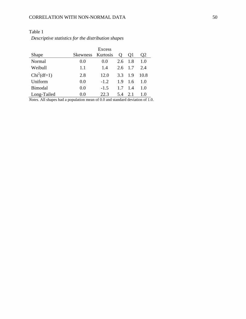
CORRELATION WITH NON-NORMAL DATA 50
Table 1
Descriptive statistics for the distribution shapes
Shape Skewness
Excess
Kurtosis Q Q1 Q2
Normal 0.0 0.0 2.6 1.8 1.0
Weibull 1.1 1.4 2.6 1.7 2.4
Chi2(df=1) 2.8 12.0 3.3 1.9 10.8
Uniform 0.0 -1.2 1.9 1.6 1.0
Bimodal 0.0 -1.5 1.7 1.4 1.0
Long-Tailed 0.0 22.3 5.4 2.1 1.0 Notes. All shapes had a population mean of 0.0 and standard deviation of 1.0.
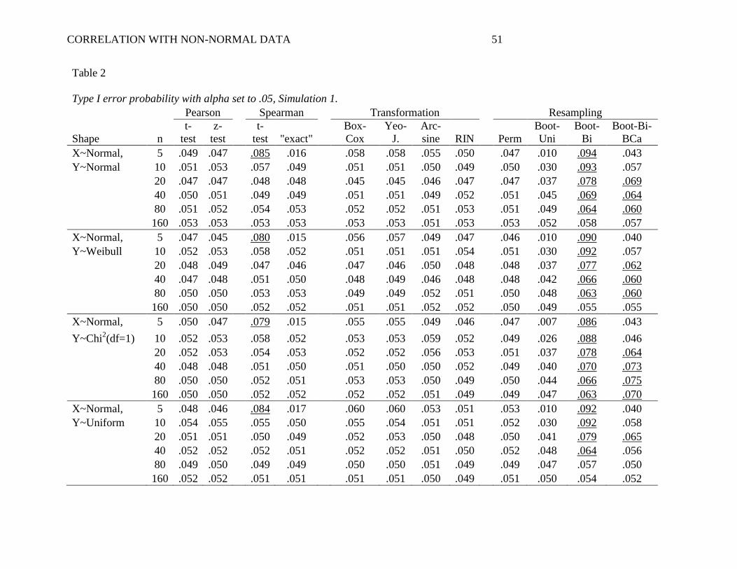
CORRELATION WITH NON-NORMAL DATA 51
Table 2
Type I error probability with alpha set to .05, Simulation 1.
Pearson
Spearman
Transformation
Resampling
Shape n
t-
test
z-
test
t-
test "exact"
Box-
Cox
Yeo-
J.
Arc-
sine RIN Perm
Boot-
Uni
Boot-
Bi
Boot-Bi-
BCa
X~Normal, 5 .049 .047
.085 .016
.058 .058 .055 .050
.047 .010 .094 .043
Y~Normal 10 .051 .053
.057 .049
.051 .051 .050 .049
.050 .030 .093 .057
20 .047 .047
.048 .048
.045 .045 .046 .047
.047 .037 .078 .069
40 .050 .051
.049 .049
.051 .051 .049 .052
.051 .045 .069 .064
80 .051 .052
.054 .053
.052 .052 .051 .053
.051 .049 .064 .060
160 .053 .053 .053 .053 .053 .053 .051 .053 .053 .052 .058 .057
X~Normal, 5 .047 .045
.080 .015
.056 .057 .049 .047
.046 .010 .090 .040
Y~Weibull 10 .052 .053
.058 .052
.051 .051 .051 .054
.051 .030 .092 .057
20 .048 .049
.047 .046
.047 .046 .050 .048
.048 .037 .077 .062
40 .047 .048
.051 .050
.048 .049 .046 .048
.048 .042 .066 .060
80 .050 .050
.053 .053
.049 .049 .052 .051
.050 .048 .063 .060
160 .050 .050 .052 .052 .051 .051 .052 .052 .050 .049 .055 .055
X~Normal, 5 .050 .047
.079 .015
.055 .055 .049 .046
.047 .007 .086 .043
Y~Chi2(df=1) 10 .052 .053
.058 .052
.053 .053 .059 .052
.049 .026 .088 .046
20 .052 .053
.054 .053
.052 .052 .056 .053
.051 .037 .078 .064
40 .048 .048
.051 .050
.051 .050 .050 .052
.049 .040 .070 .073
80 .050 .050
.052 .051
.053 .053 .050 .049
.050 .044 .066 .075
160 .050 .050 .052 .052 .052 .052 .051 .049 .049 .047 .063 .070
X~Normal, 5 .048 .046
.084 .017
.060 .060 .053 .051
.053 .010 .092 .040
Y~Uniform 10 .054 .055
.055 .050
.055 .054 .051 .051
.052 .030 .092 .058
20 .051 .051
.050 .049
.052 .053 .050 .048
.050 .041 .079 .065
40 .052 .052
.052 .051
.052 .052 .051 .050
.052 .048 .064 .056
80 .049 .050
.049 .049
.050 .050 .051 .049
.049 .047 .057 .050
160 .052 .052 .051 .051 .051 .051 .050 .049 .051 .050 .054 .052
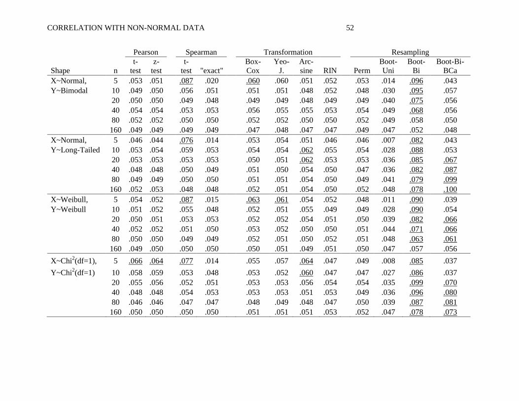
CORRELATION WITH NON-NORMAL DATA 52
Pearson Spearman Transformation Resampling
Shape n
t-
test
z-
test
t-
test "exact"
Box-
Cox
Yeo-
J.
Arc-
sine RIN Perm
Boot-
Uni
Boot-
Bi
Boot-Bi-
BCa
X~Normal, 5 .053 .051
.087 .020
.060 .060 .051 .052
.053 .014 .096 .043
Y~Bimodal 10 .049 .050
.056 .051
.051 .051 .048 .052
.048 .030 .095 .057
20 .050 .050
.049 .048
.049 .049 .048 .049
.049 .040 .075 .056
40 .054 .054
.053 .053
.056 .055 .055 .053
.054 .049 .068 .056
80 .052 .052
.050 .050
.052 .052 .050 .050
.052 .049 .058 .050
160 .049 .049 .049 .049 .047 .048 .047 .047 .049 .047 .052 .048
X~Normal, 5 .046 .044
.076 .014
.053 .054 .051 .046
.046 .007 .082 .043
Y~Long-Tailed 10 .053 .054
.059 .053
.054 .054 .062 .055
.054 .028 .088 .053
20 .053 .053
.053 .053
.050 .051 .062 .053
.053 .036 .085 .067
40 .048 .048
.050 .049
.051 .050 .054 .050
.047 .036 .082 .087
80 .049 .049
.050 .050
.051 .051 .054 .050
.049 .041 .079 .099
160 .052 .053 .048 .048 .052 .051 .054 .050 .052 .048 .078 .100
X~Weibull, 5 .054 .052
.087 .015
.063 .061 .054 .052
.048 .011 .090 .039
Y~Weibull 10 .051 .052
.055 .048
.052 .051 .055 .049
.049 .028 .090 .054
20 .050 .051
.053 .053
.052 .052 .054 .051
.050 .039 .082 .066
40 .052 .052
.051 .050
.053 .052 .050 .050
.051 .044 .071 .066
80 .050 .050
.049 .049
.052 .051 .050 .052
.051 .048 .063 .061
160 .049 .050 .050 .050 .050 .051 .049 .051 .050 .047 .057 .056
X~Chi2(df=1), 5 .066 .064
.077 .014
.055 .057 .064 .047
.049 .008 .085 .037
Y~Chi2(df=1) 10 .058 .059
.053 .048
.053 .052 .060 .047
.047 .027 .086 .037
20 .055 .056
.052 .051
.053 .053 .056 .054
.054 .035 .099 .070
40 .048 .048
.054 .053
.053 .053 .051 .053
.049 .036 .096 .080
80 .046 .046
.047 .047
.048 .049 .048 .047
.050 .039 .087 .081
160 .050 .050 .050 .050 .051 .051 .051 .053 .052 .047 .078 .073
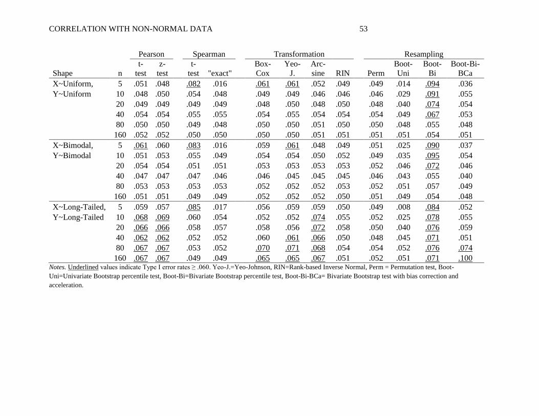
CORRELATION WITH NON-NORMAL DATA 53
Pearson Spearman Transformation Resampling
Shape n
t-
test
z-
test
t-
test "exact"
Box-
Cox
Yeo-
J.
Arc-
sine RIN Perm
Boot-
Uni
Boot-
Bi
Boot-Bi-
BCa
X~Uniform, 5 .051 .048
.082 .016
.061 .061 .052 .049
.049 .014 .094 .036
Y~Uniform 10 .048 .050
.054 .048
.049 .049 .046 .046
.046 .029 .091 .055
20 .049 .049
.049 .049
.048 .050 .048 .050
.048 .040 .074 .054
40 .054 .054
.055 .055
.054 .055 .054 .054
.054 .049 .067 .053
80 .050 .050
.049 .048
.050 .050 .051 .050
.050 .048 .055 .048
160 .052 .052 .050 .050 .050 .050 .051 .051 .051 .051 .054 .051
X~Bimodal, 5 .061 .060
.083 .016
.059 .061 .048 .049
.051 .025 .090 .037
Y~Bimodal 10 .051 .053
.055 .049
.054 .054 .050 .052
.049 .035 .095 .054
20 .054 .054
.051 .051
.053 .053 .053 .053
.052 .046 .072 .046
40 .047 .047
.047 .046
.046 .045 .045 .045
.046 .043 .055 .040
80 .053 .053
.053 .053
.052 .052 .052 .053
.052 .051 .057 .049
160 .051 .051 .049 .049 .052 .052 .052 .050 .051 .049 .054 .048
X~Long-Tailed, 5 .059 .057
.085 .017
.056 .059 .059 .050
.049 .008 .084 .052
Y~Long-Tailed 10 .068 .069
.060 .054
.052 .052 .074 .055
.052 .025 .078 .055
20 .066 .066
.058 .057
.058 .056 .072 .058
.050 .040 .076 .059
40 .062 .062
.052 .052
.060 .061 .066 .050
.048 .045 .071 .051
80 .067 .067
.053 .052
.070 .071 .068 .054
.054 .052 .076 .074
160 .067 .067 .049 .049 .065 .065 .067 .051 .052 .051 .071 .100 Notes. Underlined values indicate Type I error rates ≥ .060. Yeo-J.=Yeo-Johnson, RIN=Rank-based Inverse Normal, Perm = Permutation test, Boot-
Uni=Univariate Bootstrap percentile test, Boot-Bi=Bivariate Bootstrap percentile test, Boot-Bi-BCa= Bivariate Bootstrap test with bias correction and
acceleration.
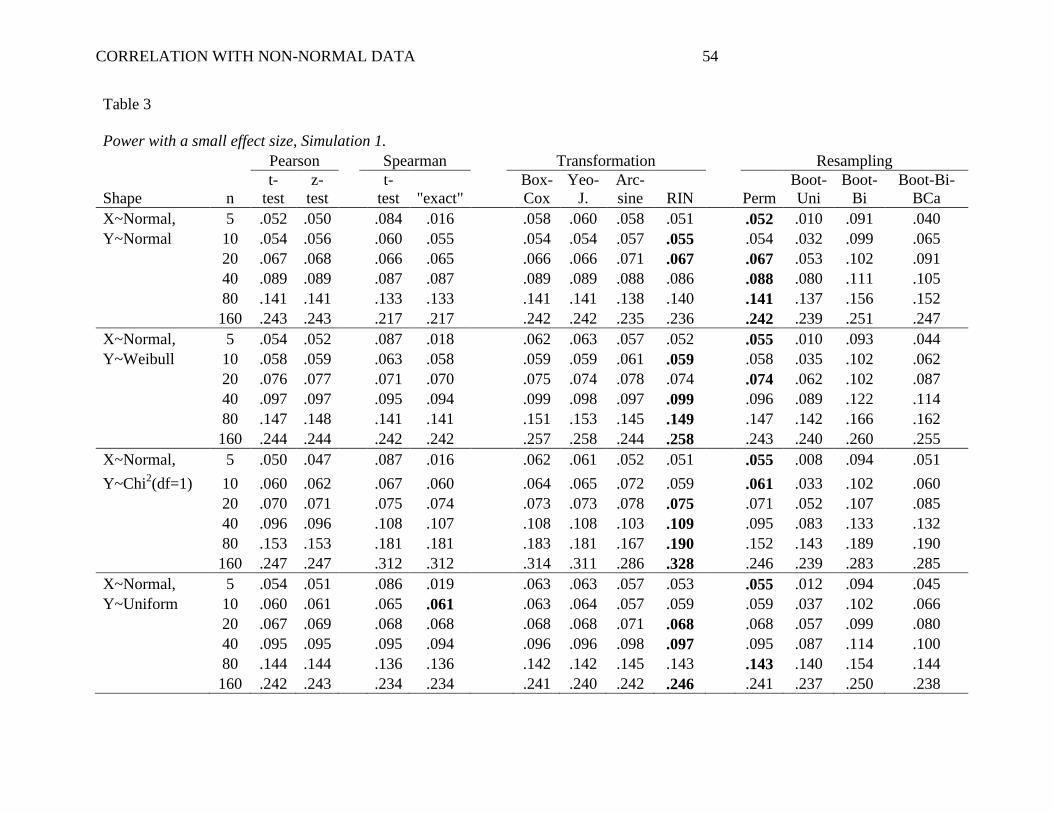
CORRELATION WITH NON-NORMAL DATA 54
Table 3
Power with a small effect size, Simulation 1.
Pearson
Spearman
Transformation
Resampling
Shape n
t-
test
z-
test
t-
test "exact"
Box-
Cox
Yeo-
J.
Arc-
sine RIN
Perm
Boot-
Uni
Boot-
Bi
Boot-Bi-
BCa
X~Normal, 5 .052 .050 .084 .016 .058 .060 .058 .051 .052 .010 .091 .040
Y~Normal 10 .054 .056
.060 .055
.054 .054 .057 .055
.054 .032 .099 .065
20 .067 .068
.066 .065
.066 .066 .071 .067
.067 .053 .102 .091
40 .089 .089
.087 .087
.089 .089 .088 .086
.088 .080 .111 .105
80 .141 .141
.133 .133
.141 .141 .138 .140
.141 .137 .156 .152
160 .243 .243 .217 .217 .242 .242 .235 .236 .242 .239 .251 .247
X~Normal, 5 .054 .052 .087 .018 .062 .063 .057 .052 .055 .010 .093 .044
Y~Weibull 10 .058 .059
.063 .058
.059 .059 .061 .059
.058 .035 .102 .062
20 .076 .077
.071 .070
.075 .074 .078 .074
.074 .062 .102 .087
40 .097 .097
.095 .094
.099 .098 .097 .099
.096 .089 .122 .114
80 .147 .148
.141 .141
.151 .153 .145 .149
.147 .142 .166 .162
160 .244 .244 .242 .242 .257 .258 .244 .258 .243 .240 .260 .255
X~Normal, 5 .050 .047
.087 .016
.062 .061 .052 .051
.055 .008 .094 .051
Y~Chi2(df=1) 10 .060 .062
.067 .060
.064 .065 .072 .059
.061 .033 .102 .060
20 .070 .071
.075 .074
.073 .073 .078 .075
.071 .052 .107 .085
40 .096 .096
.108 .107
.108 .108 .103 .109
.095 .083 .133 .132
80 .153 .153
.181 .181
.183 .181 .167 .190
.152 .143 .189 .190
160 .247 .247
.312 .312
.314 .311 .286 .328
.246 .239 .283 .285
X~Normal, 5 .054 .051 .086 .019 .063 .063 .057 .053 .055 .012 .094 .045
Y~Uniform 10 .060 .061
.065 .061
.063 .064 .057 .059
.059 .037 .102 .066
20 .067 .069
.068 .068
.068 .068 .071 .068
.068 .057 .099 .080
40 .095 .095
.095 .094
.096 .096 .098 .097
.095 .087 .114 .100
80 .144 .144
.136 .136
.142 .142 .145 .143
.143 .140 .154 .144
160 .242 .243 .234 .234 .241 .240 .242 .246 .241 .237 .250 .238
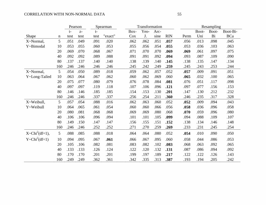
CORRELATION WITH NON-NORMAL DATA 55
Pearson
Spearman
Transformation
Resampling
Shape n
t-
test
z-
test
t-
test "exact"
Box-
Cox
Yeo-
J.
Arc-
sine RIN Perm
Boot-
Uni
Boot-
Bi
Boot-Bi-
BCa
X~Normal, 5 .051 .049
.091 .020
.062 .062 .051 .057
.056 .013 .098 .045
Y~Bimodal 10 .053 .055
.060 .053
.055 .056 .054 .055
.053 .036 .103 .063
20 .069 .070
.068 .067
.071 .070 .070 .069
.069 .061 .097 .075
40 .092 .092
.089 .088
.091 .091 .092 .094
.093 .087 .109 .090
80 .137 .137
.140 .140
.138 .139 .140 .145
.138 .135 .147 .134
160 .246 .246
.246 .246
.245 .242 .249 .259
.245 .243 .253 .244
X~Normal, 5 .054 .050 .089 .018 .059 .062 .057 .052 .057 .009 .091 .051
Y~Long-Tailed 10 .063 .064
.067 .062
.060 .062 .069 .060
.065 .032 .100 .065
20 .075 .077
.080 .079
.076 .078 .084 .081
.076 .051 .117 .098
40 .097 .097
.119 .118
.107 .106 .096 .121
.097 .077 .156 .153
80 .146 .146
.185 .185
.154 .153 .130 .201
.147 .130 .212 .232
160 .246 .246 .337 .337 .256 .254 .211 .360 .246 .235 .317 .328
X~Weibull, 5 .057 .054
.088 .016
.062 .063 .060 .052
.052 .009 .094 .043
Y~Weibull 10 .064 .065
.061 .054
.060 .060 .066 .056
.058 .036 .096 .058
20 .080 .081
.068 .068
.069 .069 .080 .068
.070 .059 .096 .080
40 .106 .106
.096 .094
.101 .101 .105 .099
.094 .088 .109 .107
80 .149 .150
.147 .147
.156 .155 .151 .152
.138 .134 .146 .148
160 .246 .246
.252 .252
.271 .270 .259 .269
.233 .231 .245 .254
X~Chi2(df=1), 5 .088 .085 .088 .018 .064 .064 .080 .052 .054 .010 .090 .050
Y~Chi2(df=1) 10 .094 .095
.067 .061
.066 .067 .095 .060
.058 .044 .086 .053
20 .105 .106
.082 .081
.083 .082 .102 .083
.068 .063 .092 .065
40 .133 .133
.126 .124
.122 .120 .132 .131
.087 .086 .094 .092
80 .170 .170
.201 .201
.199 .197 .189 .217
.122 .122 .126 .143
160 .249 .249 .362 .361 .342 .335 .313 .387 .193 .194 .205 .242
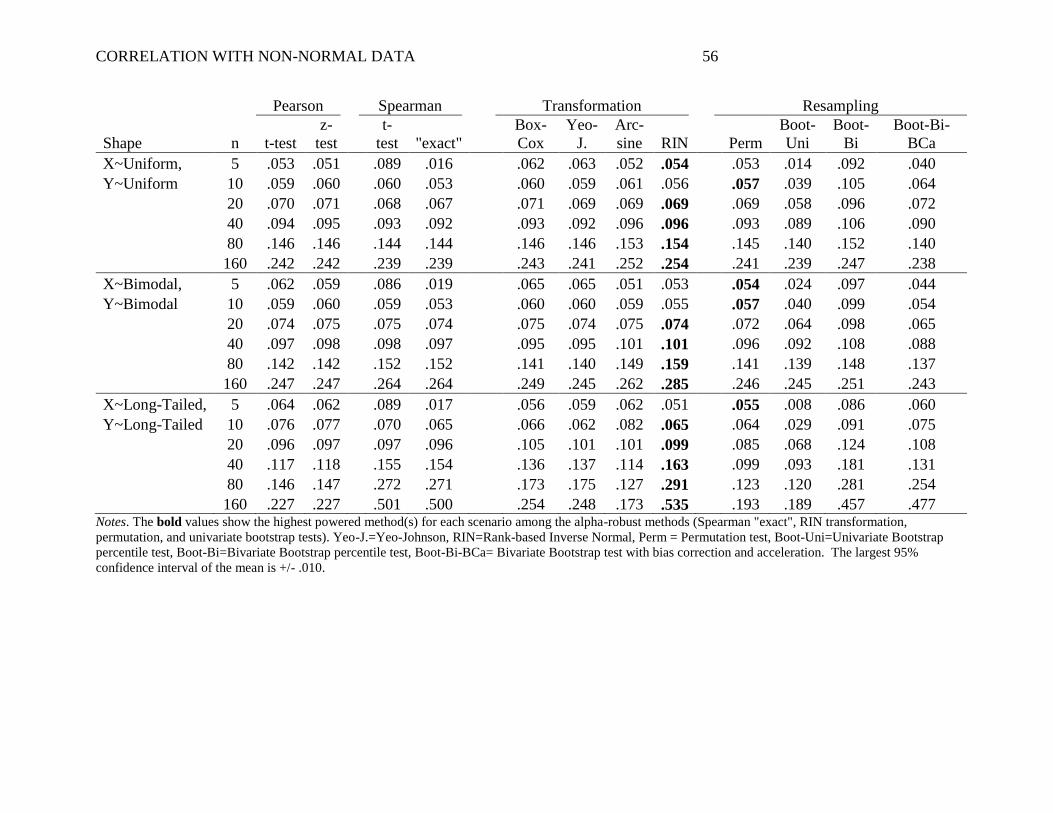
CORRELATION WITH NON-NORMAL DATA 56
Pearson
Spearman
Transformation
Resampling
Shape n t-test
z-
test
t-
test "exact"
Box-
Cox
Yeo-
J.
Arc-
sine RIN Perm
Boot-
Uni
Boot-
Bi
Boot-Bi-
BCa
X~Uniform, 5 .053 .051
.089 .016
.062 .063 .052 .054
.053 .014 .092 .040
Y~Uniform 10 .059 .060
.060 .053
.060 .059 .061 .056
.057 .039 .105 .064
20 .070 .071
.068 .067
.071 .069 .069 .069
.069 .058 .096 .072
40 .094 .095
.093 .092
.093 .092 .096 .096
.093 .089 .106 .090
80 .146 .146
.144 .144
.146 .146 .153 .154
.145 .140 .152 .140
160 .242 .242
.239 .239
.243 .241 .252 .254
.241 .239 .247 .238
X~Bimodal, 5 .062 .059 .086 .019 .065 .065 .051 .053 .054 .024 .097 .044
Y~Bimodal 10 .059 .060
.059 .053
.060 .060 .059 .055
.057 .040 .099 .054
20 .074 .075
.075 .074
.075 .074 .075 .074
.072 .064 .098 .065
40 .097 .098
.098 .097
.095 .095 .101 .101
.096 .092 .108 .088
80 .142 .142
.152 .152
.141 .140 .149 .159
.141 .139 .148 .137
160 .247 .247 .264 .264 .249 .245 .262 .285 .246 .245 .251 .243
X~Long-Tailed, 5 .064 .062 .089 .017 .056 .059 .062 .051 .055 .008 .086 .060
Y~Long-Tailed 10 .076 .077
.070 .065
.066 .062 .082 .065
.064 .029 .091 .075
20 .096 .097
.097 .096
.105 .101 .101 .099
.085 .068 .124 .108
40 .117 .118
.155 .154
.136 .137 .114 .163
.099 .093 .181 .131
80 .146 .147
.272 .271
.173 .175 .127 .291
.123 .120 .281 .254
160 .227 .227 .501 .500 .254 .248 .173 .535 .193 .189 .457 .477 Notes. The bold values show the highest powered method(s) for each scenario among the alpha-robust methods (Spearman "exact", RIN transformation,
permutation, and univariate bootstrap tests). Yeo-J.=Yeo-Johnson, RIN=Rank-based Inverse Normal, Perm = Permutation test, Boot-Uni=Univariate Bootstrap
percentile test, Boot-Bi=Bivariate Bootstrap percentile test, Boot-Bi-BCa= Bivariate Bootstrap test with bias correction and acceleration. The largest 95%
confidence interval of the mean is +/- .010.
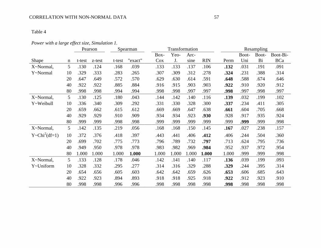
CORRELATION WITH NON-NORMAL DATA 57
Table 4
Power with a large effect size, Simulation 1.
Pearson
Spearman
Transformation
Resampling
Shape n t-test z-test
t-test "exact"
Box-
Cox
Yeo-
J.
Arc-
sine RIN
Perm
Boot-
Uni
Boot-
Bi
Boot-Bi-
BCa
X~Normal, 5 .130 .124 .168 .039 .133 .133 .137 .106 .132 .031 .191 .091
Y~Normal 10 .329 .333
.283 .265
.307 .309 .312 .278
.324 .231 .388 .314
20 .647 .649
.572 .570
.629 .630 .614 .591
.648 .588 .674 .646
40 .922 .922
.885 .884
.916 .915 .903 .903
.922 .910 .920 .912
80 .998 .998 .994 .994 .998 .998 .997 .997 .998 .997 .998 .997
X~Normal, 5 .130 .125
.180 .043
.144 .142 .140 .116
.139 .032 .199 .102
Y~Weibull 10 .336 .340
.309 .292
.331 .330 .328 .300
.337 .234 .411 .305
20 .659 .662
.615 .612
.669 .669 .647 .638
.661 .604 .705 .668
40 .929 .929
.910 .909
.934 .934 .923 .930
.928 .917 .935 .924
80 .999 .999
.998 .998
.999 .999 .999 .999
.999 .999 .999 .998
X~Normal, 5 .142 .135 .219 .056 .168 .168 .150 .145 .167 .027 .238 .157
Y~Chi2(df=1) 10 .372 .376
.418 .397
.443 .441 .406 .412
.406 .244 .504 .360
20 .699 .702
.775 .773
.796 .789 .732 .797
.713 .624 .795 .736
40 .949 .950
.978 .978
.983 .982 .969 .984
.952 .937 .972 .954
80 1.000 1.000 1.000 1.000 1.000 1.000 1.000 1.000 1.000 .999 .999 .998
X~Normal, 5 .133 .128
.178 .046
.142 .141 .140 .117
.136 .039 .199 .093
Y~Uniform 10 .328 .332
.295 .277
.314 .316 .329 .288
.329 .244 .395 .314
20 .654 .656
.605 .603
.642 .642 .659 .626
.653 .606 .685 .643
40 .922 .923
.894 .893
.918 .918 .925 .918
.922 .912 .923 .910
80 .998 .998 .996 .996 .998 .998 .998 .998 .998 .998 .998 .998
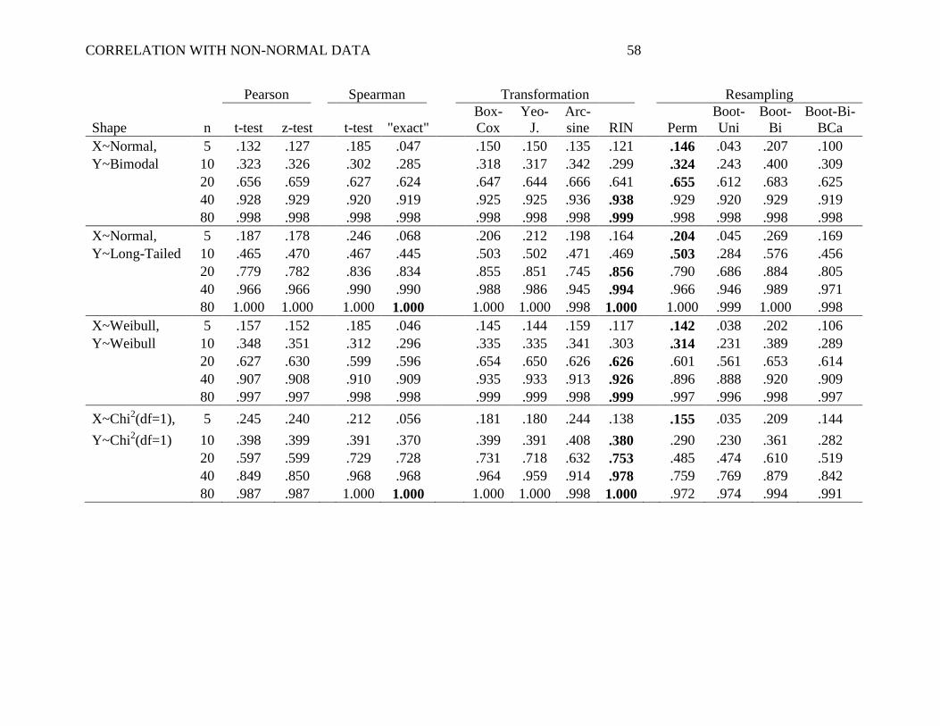
CORRELATION WITH NON-NORMAL DATA 58
Pearson
Spearman
Transformation
Resampling
Shape n t-test z-test
t-test "exact"
Box-
Cox
Yeo-
J.
Arc-
sine RIN
Perm
Boot-
Uni
Boot-
Bi
Boot-Bi-
BCa
X~Normal, 5 .132 .127 .185 .047 .150 .150 .135 .121 .146 .043 .207 .100
Y~Bimodal 10 .323 .326
.302 .285
.318 .317 .342 .299
.324 .243 .400 .309
20 .656 .659
.627 .624
.647 .644 .666 .641
.655 .612 .683 .625
40 .928 .929
.920 .919
.925 .925 .936 .938
.929 .920 .929 .919
80 .998 .998 .998 .998 .998 .998 .998 .999 .998 .998 .998 .998
X~Normal, 5 .187 .178
.246 .068
.206 .212 .198 .164
.204 .045 .269 .169
Y~Long-Tailed 10 .465 .470
.467 .445
.503 .502 .471 .469
.503 .284 .576 .456
20 .779 .782
.836 .834
.855 .851 .745 .856
.790 .686 .884 .805
40 .966 .966
.990 .990
.988 .986 .945 .994
.966 .946 .989 .971
80 1.000 1.000
1.000 1.000
1.000 1.000 .998 1.000
1.000 .999 1.000 .998
X~Weibull, 5 .157 .152 .185 .046 .145 .144 .159 .117 .142 .038 .202 .106
Y~Weibull 10 .348 .351
.312 .296
.335 .335 .341 .303
.314 .231 .389 .289
20 .627 .630
.599 .596
.654 .650 .626 .626
.601 .561 .653 .614
40 .907 .908
.910 .909
.935 .933 .913 .926
.896 .888 .920 .909
80 .997 .997 .998 .998 .999 .999 .998 .999 .997 .996 .998 .997
X~Chi2(df=1), 5 .245 .240
.212 .056
.181 .180 .244 .138
.155 .035 .209 .144
Y~Chi2(df=1) 10 .398 .399
.391 .370
.399 .391 .408 .380
.290 .230 .361 .282
20 .597 .599
.729 .728
.731 .718 .632 .753
.485 .474 .610 .519
40 .849 .850
.968 .968
.964 .959 .914 .978
.759 .769 .879 .842
80 .987 .987 1.000 1.000 1.000 1.000 .998 1.000 .972 .974 .994 .991
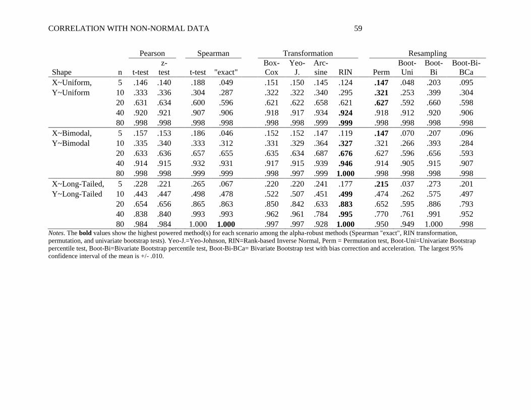
CORRELATION WITH NON-NORMAL DATA 59
Pearson
Spearman
Transformation
Resampling
Shape n t-test
z-
test
t-test "exact"
Box-
Cox
Yeo-
J.
Arc-
sine RIN
Perm
Boot-
Uni
Boot-
Bi
Boot-Bi-
BCa
X~Uniform, 5 .146 .140 .188 .049 .151 .150 .145 .124 .147 .048 .203 .095
Y~Uniform 10 .333 .336
.304 .287
.322 .322 .340 .295
.321 .253 .399 .304
20 .631 .634
.600 .596
.621 .622 .658 .621
.627 .592 .660 .598
40 .920 .921
.907 .906
.918 .917 .934 .924
.918 .912 .920 .906
80 .998 .998 .998 .998 .998 .998 .999 .999 .998 .998 .998 .998
X~Bimodal, 5 .157 .153
.186 .046
.152 .152 .147 .119
.147 .070 .207 .096
Y~Bimodal 10 .335 .340
.333 .312
.331 .329 .364 .327
.321 .266 .393 .284
20 .633 .636
.657 .655
.635 .634 .687 .676
.627 .596 .656 .593
40 .914 .915
.932 .931
.917 .915 .939 .946
.914 .905 .915 .907
80 .998 .998
.999 .999
.998 .997 .999 1.000
.998 .998 .998 .998
X~Long-Tailed, 5 .228 .221 .265 .067 .220 .220 .241 .177 .215 .037 .273 .201
Y~Long-Tailed 10 .443 .447
.498 .478
.522 .507 .451 .499
.474 .262 .575 .497
20 .654 .656
.865 .863
.850 .842 .633 .883
.652 .595 .886 .793
40 .838 .840
.993 .993
.962 .961 .784 .995
.770 .761 .991 .952
80 .984 .984 1.000 1.000 .997 .997 .928 1.000 .950 .949 1.000 .998 Notes. The bold values show the highest powered method(s) for each scenario among the alpha-robust methods (Spearman "exact", RIN transformation,
permutation, and univariate bootstrap tests). Yeo-J.=Yeo-Johnson, RIN=Rank-based Inverse Normal, Perm = Permutation test, Boot-Uni=Univariate Bootstrap
percentile test, Boot-Bi=Bivariate Bootstrap percentile test, Boot-Bi-BCa= Bivariate Bootstrap test with bias correction and acceleration. The largest 95%
confidence interval of the mean is +/- .010.
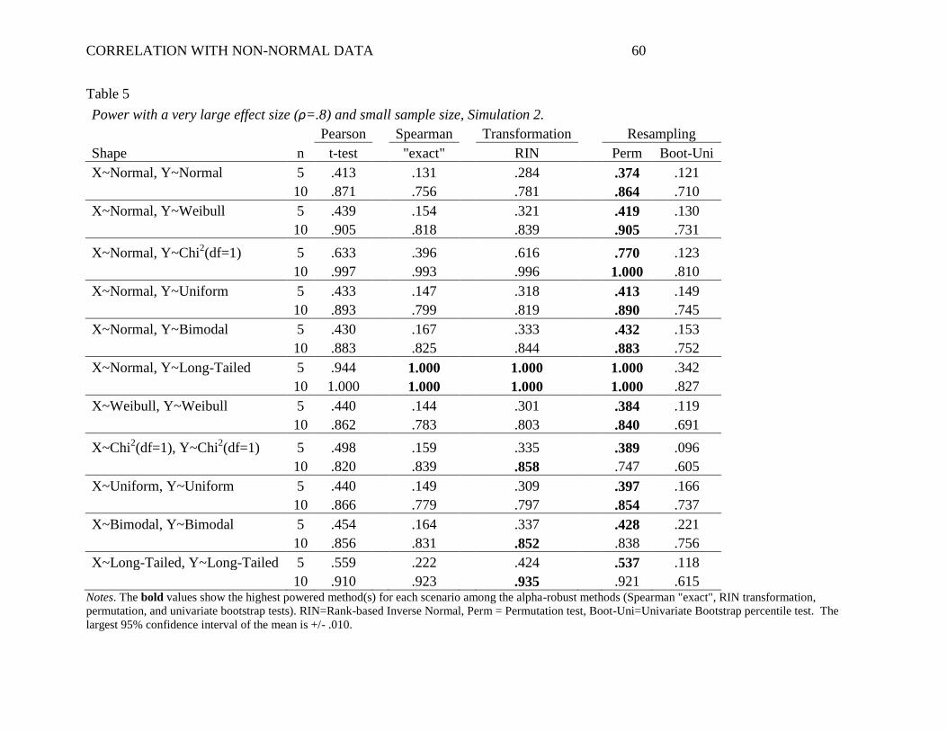
CORRELATION WITH NON-NORMAL DATA 60
Table 5
Power with a very large effect size (ρ=.8) and small sample size, Simulation 2.
Pearson
Spearman
Transformation
Resampling
Shape n t-test "exact"
RIN
Perm Boot-Uni
X~Normal, Y~Normal 5 .413 .131 .284 .374 .121
10 .871 .756 .781 .864 .710
X~Normal, Y~Weibull 5 .439
.154 .321 .419 .130
10 .905
.818 .839 .905 .731
X~Normal, Y~Chi2(df=1) 5 .633 .396 .616 .770 .123
10 .997 .993 .996 1.000 .810
X~Normal, Y~Uniform 5 .433
.147 .318 .413 .149
10 .893
.799 .819 .890 .745
X~Normal, Y~Bimodal 5 .430 .167 .333 .432 .153
10 .883 .825 .844 .883 .752
X~Normal, Y~Long-Tailed 5 .944
1.000 1.000 1.000 .342
10 1.000
1.000 1.000 1.000 .827
X~Weibull, Y~Weibull 5 .440 .144 .301 .384 .119
10 .862 .783 .803 .840 .691
X~Chi2(df=1), Y~Chi
2(df=1) 5 .498
.159 .335 .389 .096
10 .820
.839 .858 .747 .605
X~Uniform, Y~Uniform 5 .440 .149 .309 .397 .166
10 .866 .779 .797 .854 .737
X~Bimodal, Y~Bimodal 5 .454
.164 .337 .428 .221
10 .856
.831
.852
.838 .756
X~Long-Tailed, Y~Long-Tailed 5 .559 .222 .424 .537 .118
10 .910 .923 .935 .921 .615 Notes. The bold values show the highest powered method(s) for each scenario among the alpha-robust methods (Spearman "exact", RIN transformation,
permutation, and univariate bootstrap tests). RIN=Rank-based Inverse Normal, Perm = Permutation test, Boot-Uni=Univariate Bootstrap percentile test. The
largest 95% confidence interval of the mean is +/- .010.
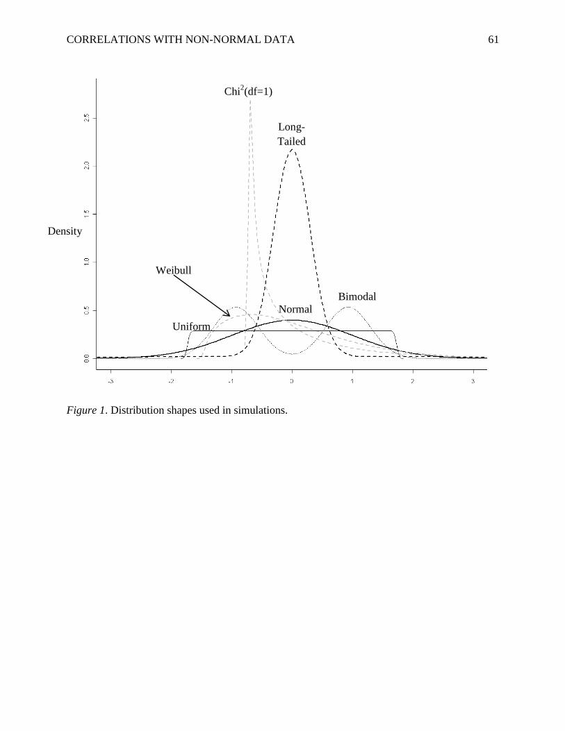
CORRELATIONS WITH NON-NORMAL DATA 61
Figure 1. Distribution shapes used in simulations.
Density
Long-
Tailed
Normal
Chi2(df=1)
Weibull
Bimodal
Uniform
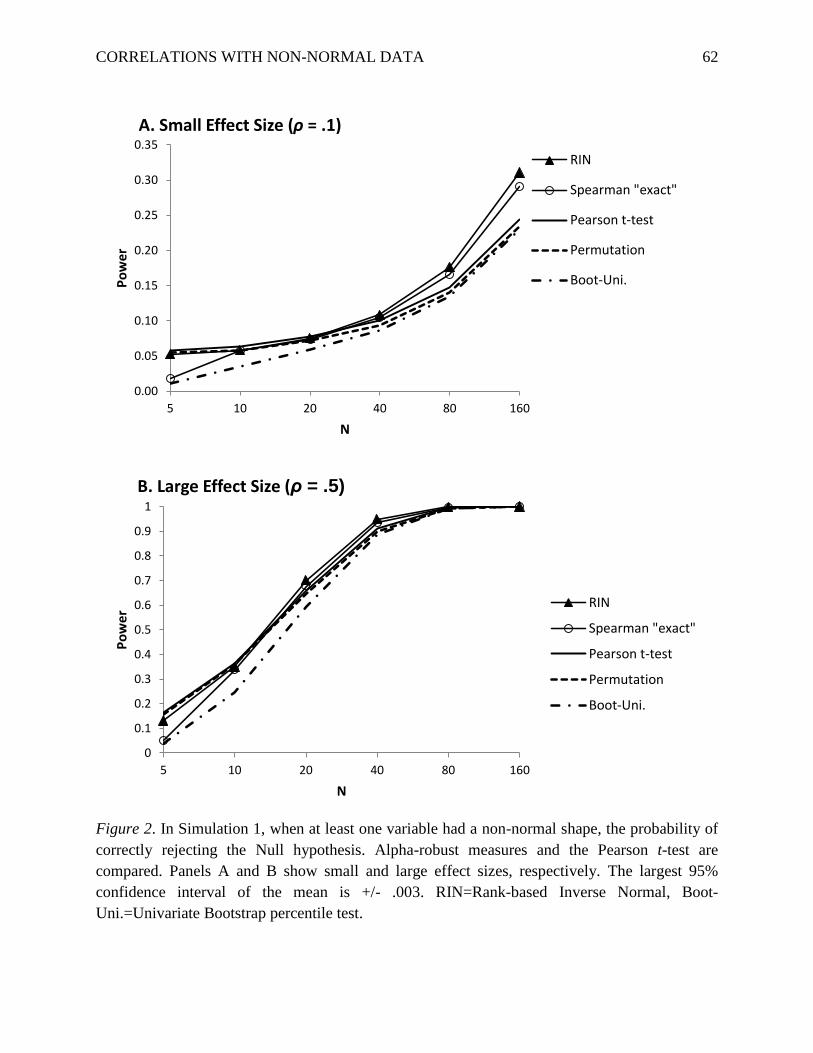
CORRELATIONS WITH NON-NORMAL DATA 62
Figure 2. In Simulation 1, when at least one variable had a non-normal shape, the probability of
correctly rejecting the Null hypothesis. Alpha-robust measures and the Pearson t-test are
compared. Panels A and B show small and large effect sizes, respectively. The largest 95%
confidence interval of the mean is +/- .003. RIN=Rank-based Inverse Normal, Boot-
Uni.=Univariate Bootstrap percentile test.
0.00
0.05
0.10
0.15
0.20
0.25
0.30
0.35
5 10 20 40 80 160
Po
wer
N
A. Small Effect Size (ρ = .1)
RIN
Spearman "exact"
Pearson t-test
Permutation
Boot-Uni.
0
0.1
0.2
0.3
0.4
0.5
0.6
0.7
0.8
0.9
1
5 10 20 40 80 160
Po
wer
N
B. Large Effect Size (ρ = .5)
RIN
Spearman "exact"
Pearson t-test
Permutation
Boot-Uni.


![[Normal Probability Curve and Correlation] definition of](https://img.pdfslide.us/doc/110x75/615bc93a0cd15d21e0638188/normal-probability-curve-and-correlation-definition-of-.jpg)