Rubber Band Recoil - HAL :: Accueil

HAL Id: hal-00087503https://hal.archives-ouvertes.fr/hal-00087503

Submitted on 25 Jul 2006

HAL is a multi-disciplinary open accessarchive for the deposit and dissemination of sci-entific research documents, whether they are pub-lished or not. The documents may come fromteaching and research institutions in France orabroad, or from public or private research centers.

L’archive ouverte pluridisciplinaire HAL, estdestinée au dépôt et à la diffusion de documentsscientifiques de niveau recherche, publiés ou non,émanant des établissements d’enseignement et derecherche français ou étrangers, des laboratoirespublics ou privés.

Rubber Band RecoilRomain Vermorel, Nicolas Vandenberghe, Emmanuel Villermaux

To cite this version:Romain Vermorel, Nicolas Vandenberghe, Emmanuel Villermaux. Rubber Band Recoil. Pro-ceedings of the Royal Society of London, Royal Society, The, 2007, 463 (2079), pp.641-658.<10.1098/rspa.2006.1781>. <hal-00087503>

https://hal.archives-ouvertes.fr/hal-00087503

https://hal.archives-ouvertes.fr

Rubber Band Recoil

By R. Vermorel, N. Vandenberghe and E. Villermaux†Universite de Provence, IRPHE, 49, rue Frederic Joliot-Curie

13384 Marseille Cedex 13, France

When an initially stretched rubber band is suddenly released at one end, an axial-stress front propagating at the celerity of sound separates a free and a stretcheddomain of the elastic material. As soon as it reaches the clamped end, the frontrebounds and a compression front propagates backward. When the length of thecompressed area exceeds Euler critical length, a dynamic buckling instability devel-ops. The rebound is analysed using Saint-Venant’s theory of impacts and we use adynamical extension of the Euler-Bernoulli beam equation to obtain a relation be-tween the buckled wavelength, the initial stretching and the rubber band thickness.The influence of an external fluid medium is also considered: due to added massand viscosity the instability growth rate decreases. With a high viscosity, the axial-stress front spreads because of viscous frictional forces during the release phase. Asa result, the selected wavelength increases significantly.

Keywords: Rubber band, elastic instability, dynamic buckling

1. Introduction

In his classical treatment of the elastica, Euler (1744) proved that for a given lengthand for given boundary conditions, there exists a critical load at which a rod buckles.Among the different possible bent shapes, only the one with the smallest numberof inflections is stable i.e. the shape corresponding to the fundamental flexuralmode (see e.g. Love (1944)). Thus the only characteristic length associated withthe buckling instability is the length of the rod itself.

However, when a compressive load several times higher than the Euler criticalforce is suddenly applied to an elastica at rest, the buckling instability developsdynamically, and a characteristic wavelength is selected. Lindberg (1965) proposeda simple model to predict the amplified wavelength. Using Euler-Bernoulli theoryfor the elastic beam, he studied the growth of the different flexural modes of thebeam. The theory predicts that the most amplified wavelength decreases like theinverse square root of the compression strain. Lindberg also devised an ingeniousway to determine the buckled wavelength from experiments on metallic elastic beamand on rubber bands. In the case of the metallic beam he found a fair agreementwith theory, while in the case of the rubber band, discrepancies were stronger: themeasured wavelength was 70 percent higher than predicted for reasons that werenot elucidated.

The aim of the present work is to study in details the dynamic buckling in-stability responsible for the recoil of a rubber band. Indeed the rubber band isan interesting system for the study of dynamic buckling because the characteristic

† Also at: Institut Universitaire de France

Article submitted to Royal Society TEX Paper

2 R.Vermorel, N.Vandenberghe and E.Villermaux

speed of sound in rubber is moderate (about 40 m s−1) and strains and displace-ments can be large. It also represents a simple case study of more general situationswhere flexural waves and compression waves are coupled, as those encountered inthe related problem of brittle rods fragmentation under impact (Gladden et al.(2005)). The question is envisaged in its most general setting, including the influ-ence of a surrounding medium as we perform experiments in air, and in liquids,namely water and water-glycerol mixtures to investigate the effect of added massand fluid viscosity.

2. Experimental set-up

We first consider the recoil of a cantilever rubber band. One end of the rubber bandis firmly clamped on the experimentation table. The operator holds the free end,stretches the elastic to the desired length, and releases it suddenly. A setup wasalso designed that allowed to stretch and release the rubber band from both endssimultaneously to study the influence of the boundary conditions. A thin fishingline is glued on both ends of the elastic in such a way that the line and the elasticmaterial form a loop. This loop is placed around two pulley. Thus the operator canstretch and release the rubber band just by pulling and dropping the fishing line.

The elastics were cut from natural latex rubber sheets of different thicknessesfrom 0.254 mm up to 1.270 mm. The characteristic length and width of the rubberbands are l0 = 150 mm and b = 4 mm. Measuring the force-extension curve, thestatic stretching test reveals that in the range of stretching between 0 and 100percent, the elastic behavior of the rubber remains linear (within 3 percent) with aYoung modulus E = 1.5 MPa and no significant hysteretic behaviour i.e. or stresssoftening of the rubber (Bouasse and Carriere (1903), also called Mullins effect afterMullins (1947)) were observed. For higher stretching, significant deviation from theideal Hookean behavior was observed and in most experiments the stretching hasbeen limited to the range 0 to 100 percent. The density of the rubber is ρ =990 kg m−3 and thus the nominal wave speed for longitudinal disturbances is c =(E/ρ)1/2 = 39 m s−1.

All diagnostics are based on quantitative image analysis, resolved in time, usinga Phantom V5 high-speed video camera to record movies at typical frame rates of10,000 up to 30,000 frames per second. The rubber band is illuminated from behindusing a white light source and a diffusing screen or by direct lighting using a blackor white background. Regularly spaced marks are drawn on the elastic to followthe motion of the material points.

In order to study the influence of the external medium, experiments were alsoconducted with the set-up immersed in a tank filled with water or with water-glycerol mixtures of controlled viscosity. Viscosities of the mixture were measuredusing a Couette viscosimeter and we used viscosities from η = 1.0 10−3 Pa s (purewater) up to η = 6.5 10−1 Pa s.

Article submitted to Royal Society

Rubber Band Recoil 3

( i )

( ii )

( iii )

( iv )

( v )

( vi )

( vii )

( viii )

( ix )

( x )1 cm

( i )

( ii )

( iii )

( iv )

( v )

( vi )

( vii )

( viii )

( ix )

1 cm

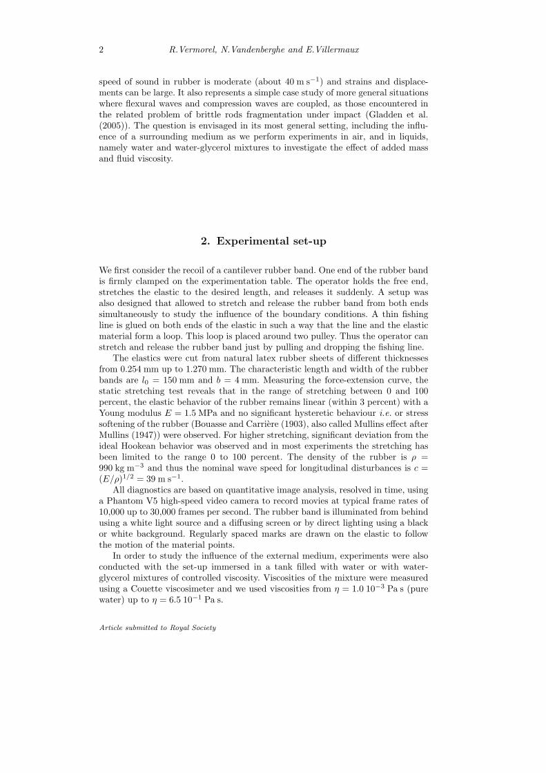
Figure 1. Top: front propagation in a clamped rubberband with initial stretch ǫ0 = 1.Arrows mark the front position. (i) to (vi) The front propagates towards the clamped endand drags the free region. (vii) When the front reaches the clamped end, the strain-freerubber band moves towards the clamped end. (viii) to (x) After impact, a compressivefront propagates backward and triggers a dynamic buckling instability. Time goes fromtop to bottom by steps of 350 µs. A movie showing the front propagation is includedin the electronic supplementary materials. Bottom: fronts propagation in a rubber bandsimultaneously released from both ends. The front propagate towards the middle of theelastic. The initial stretch is ǫ0 = 1. Arrows mark the positions of the fronts. (vi) whenthe fronts cross each other, compressive fronts set out from the middle ((vii) to(ix)) andtrigger buckling. Time goes from top to bottom by steps of 320 µs.

3. Recoil of a rubber band in air

(a) Phenomenology

Stretching and releasing a rubber band is a common experience. The typicaltimescale of this phenomenon is l0/c ≈ 3.8 ms, hence the use of high speed imaging.



1 cm

λ/2

( i )

( ii )

( iii )

( iv )

( v )

1 cm

λ/2

( i )

( ii )

( iii )

( iv )

( v )

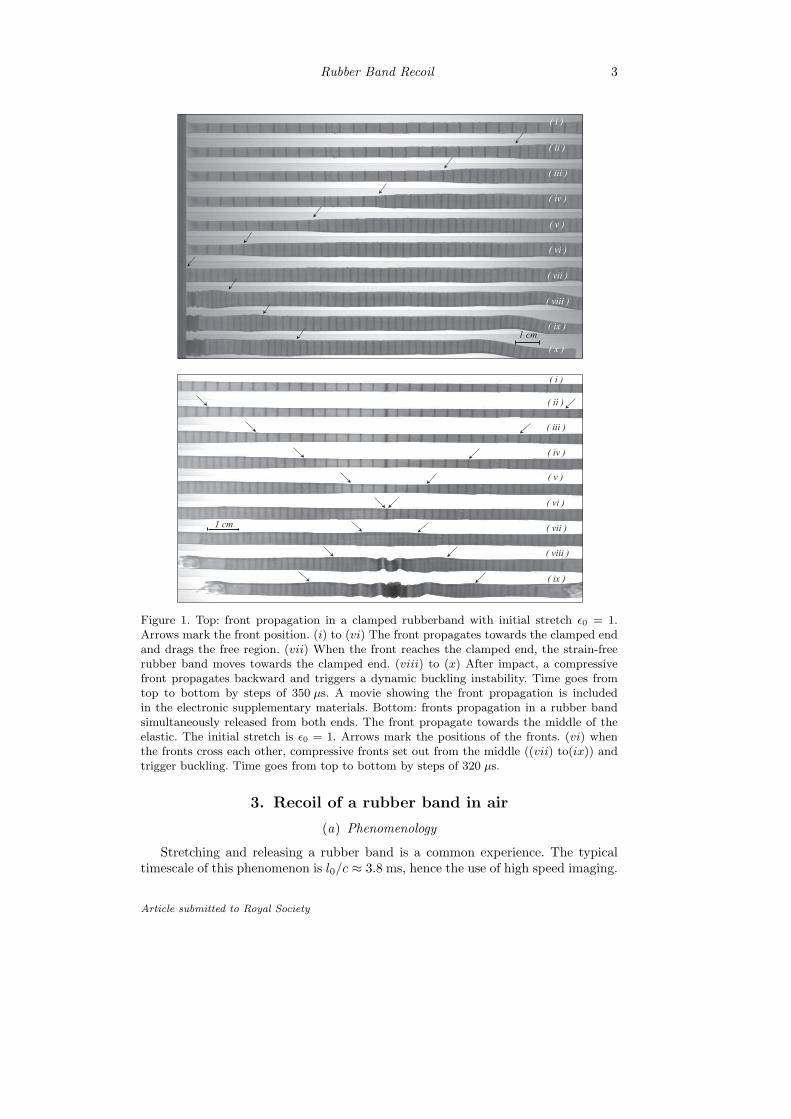
Figure 2. Left: Early stages of the dynamic buckling of a clamped rubber band. Timegoes from top to bottom by steps of 117 µs. The initial stretch is ǫ0 = 0.3. Right: Earlystages of the dynamic buckling of a rubber band simultaneously released from both ends.Time goes from top to bottom by steps of 130 µs. The initial stretch is ǫ0 = 0.2. A movieshowing the dynamic buckling is included in the electronic supplementary materials.

When the tension is suddenly released, a front propagates towards the clamped end(see figure 1, images (i) to (vi)) at the celerity c in the material. The front separatestwo regions: a stress-free area between the free end and the front, and a stretchedarea between the front and the clamped end. As the front propagates it drags thefree region down to the clamped end at velocity V , which is a fraction of c. Whenthe front reaches the clamped end, the whole rubber band is free, moving towardsthe table at velocity V (figure 1 (vii)).

The configuration is then equivalent to a free rubber band moving at velocityV impacting a rigid surface (see Saint-Venant and Flamand (1883) and referencestherein). A compressive front propagates backward (i.e. towards the free end) atspeed c in the frame of the rubber band (figure 1 (viii) to (x)). Between the clampedend and the front, the elastic is compressed. As soon as the compressive front hascovered a critical distance from the clamped end, the compressive stress is appliedto a region long enough to trigger off a buckling instability. The elastic startsto bend with a well defined wavelength (figure 2 (iv)). The first complete halfwavelength appearing during the dynamic buckling instability will be refered toas the half buckled wavelength. In later times the front propagates towards thefree end inducing more bending of the rubber band. We will focus on the first halfwavelength only, because the subsequent dynamics becomes more complicated. Inparticular, near the clamped end, the transverse displacement resulting from thebuckling is coupled to the propagation of the longitudinal wave.

To check the influence of the boundary conditions on the dynamics, we per-formed a similar experiment with a rubber band simultaneously released from bothends. Two fronts propagate towards the middle of the elastic. When the frontsreach the middle, the rubber band is stress-free but its two halves are movingwith opposite velocities V and −V . The configuration is then equivalent to theclassical problem of two rods impacting each other. Compressive fronts propagateaway from the junction (i.e the middle of the rubber band), triggering the dynamicbuckling instability in both sides of the rubber band and a selected wavelength isobserved. Measurements show that the dynamics is strictly identical to the case of



0 φ(t)

c V

ε = ε0

ε = 0

( i )

x

ξ ( x, t )

b

h

( iii )

0

c V

ε = − ε0 / ( 1+ ε

0 ) ε = 0

( ii )φ(t)

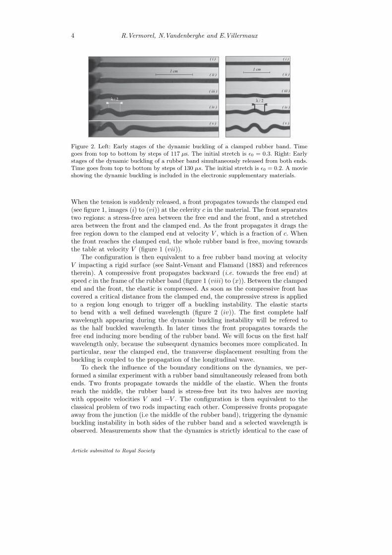
Figure 3. (i) Schematic of the stress free front propagation. ℓ is the length of the stretchedrubber band. φ is the position of the front. The stress-free front propagates towards theclamped end at speed of sound c and it drags the free region with a constant velocity V .(ii) The rebounding front propagating backward. (iii) Schematics of the dynamic bucklingof a rubber band. b and h are the width and the thickness of the band. ξ is the transversedisplacement, function of the longitudinal coordinate x and on the time t.

the clamped rubber band for low stretching (less than 50 %). However, for higherstretching, the friction of the fishing line as it slides against the axes results in aslight decrease of the velocity of the free regions of the rubber band. Thereforeall the measurements reported in this paper were obtained with the more reliableclamped-free configuration.

(b) Compression front

The rubber band is modeled as a hookean elastic rod experiencing small strain.We neglect the effect of lateral inertia in the propagation and we use the smallstrain hypothesis. Thus longitudinal perturbations are governed by the linear waveequation with the propagation speed c.

Let ℓ be the length of the stretched rubber band and ℓ0 its length at rest. Theinitial strain ǫ0 is

ǫ0 =ℓ − ℓ0

ℓ0(3.1)

The front is a discontinuity that separates a strain-free region and a stretched regionin which ǫ = ǫ0 (figure 3 (i)). The front propagates at speed c and it reaches theanchor point at time ti = ℓ/c. Then the elastic is strain-free and its length is l0. Vbeing the speed of the free end, we have ℓ − ℓ0 = −V ti and thus we obtain that

V = −{

ℓ − ℓ0ℓ

}

c = −{

ǫ01 + ǫ0

}

c (3.2)

This relation holds for all material points in the free region.When the free front reaches the clamped end, the whole rubber band is strain-

free and translates at speed V . Thus the problem is equivalent to a rubber bandimpacting a rigid surface at speed V . Let ζ(x, t) be the longitudinal displacementin the rubber band. x is the coordinate of a material point along the rod withx = 0 being the anchor point. When the front reaches the x = 0 position, all the



0

0.1

0.2

0.3

0.4

0.5

0.6

0.1 0.2 0.3 0.4 0.5 0.6

V/c

ε0/( 1 +ε0)0

X (cm)

ε( i ) ( ii )

0

0.2

0.4

0.6

0.8

1

05 10 15 20 25 30

0 0.2 0.4

c (m

.s-1)

ε0 /( 1 + ε0 )

35

40

45

50

0.6

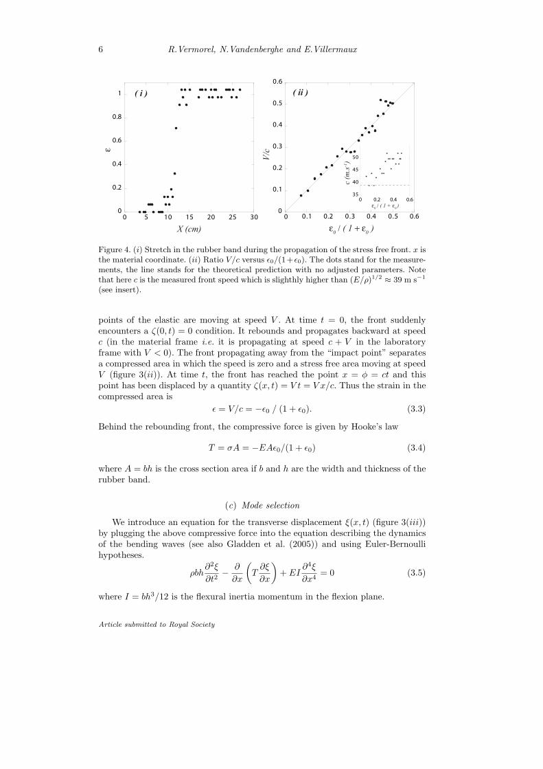
Figure 4. (i) Stretch in the rubber band during the propagation of the stress free front. x isthe material coordinate. (ii) Ratio V/c versus ǫ0/(1+ǫ0). The dots stand for the measure-ments, the line stands for the theoretical prediction with no adjusted parameters. Notethat here c is the measured front speed which is slighthly higher than (E/ρ)1/2

≈ 39 m s−1

(see insert).

points of the elastic are moving at speed V . At time t = 0, the front suddenlyencounters a ζ(0, t) = 0 condition. It rebounds and propagates backward at speedc (in the material frame i.e. it is propagating at speed c + V in the laboratoryframe with V < 0). The front propagating away from the “impact point” separatesa compressed area in which the speed is zero and a stress free area moving at speedV (figure 3(ii)). At time t, the front has reached the point x = φ = ct and thispoint has been displaced by a quantity ζ(x, t) = V t = V x/c. Thus the strain in thecompressed area is

ǫ = V/c = −ǫ0 / (1 + ǫ0). (3.3)

Behind the rebounding front, the compressive force is given by Hooke’s law

T = σA = −EAǫ0/(1 + ǫ0) (3.4)

where A = bh is the cross section area if b and h are the width and thickness of therubber band.

(c) Mode selection

We introduce an equation for the transverse displacement ξ(x, t) (figure 3(iii))by plugging the above compressive force into the equation describing the dynamicsof the bending waves (see also Gladden et al. (2005)) and using Euler-Bernoullihypotheses.

ρbh∂2ξ

∂t2− ∂

∂x

(

T∂ξ

∂x

)

+ EI∂4ξ

∂x4= 0 (3.5)

where I = bh3/12 is the flexural inertia momentum in the flexion plane.



We look for solutions of the form ξ(x, t) = ξ0 exp(ikx − iωt). With T constantalong the rod, the dispersion relation reads

ω2 =EI

ρbhk2

{

k2 +T

EI

}

(3.6)

For a compressive force, T is negative. Unstable modes have wave numbers in therange 0 to kc where kc is the marginal wavenumber,

kc =

√

|T |EI

(3.7)

The most amplified wave number is km = kc/√

2, so that, making use of equation(3.4) for T , the most amplified wavelength writes, Mutatis Mutandis

λm = πh

√

2

3

√

1 + ǫ0ǫ0

(3.8)

and its associated growth rate is

σm =√

3ǫ0

1 + ǫ0

c

h(3.9)

The selected mode depends on both the material elastic properties and intensityof the compression, but since the compression is itself a function of the materialelasticity, a cancellation effect makes λm depend on geometrical parameters only,namely the thickness of the rubber band and initial stretching.

Of course, this naive expectation assumes that the compression front has trav-elled by a distance at least equal to λm during a time lapse given by σ−1

m . A moregeneral mode selection criterion would thus be that the amplified wavenumber k isthe one for which

τ(k)c ≃ k−1 (3.10)

and k = km otherwise if τ(k)c ≫ k−1. There, τ(k) is the instability timescale asso-ciated with k through the dispersion relation (3.6) such that τ(k)−1 = Re{−iω}.

The above reasonings are made within the long wave approximation (kh ≪ 1)and disregard three dimensional effects when the wavelength becomes of the orderof the thickness h, as it is nevertheless the case for the higher initial elongations ǫ0.We also do not account for any coupling between the instability development andthe compression force, nor any nonlinear elastic response of the material.

(d) Experimental results

To measure the propagation speeds, we draw regularly spaced marks along therubber band (figure 1). The theoretical value of the front velocity for the rubberbands that we used in the experiments is 39 m s−1, which is in agreement with themeasurements for small initial stretching. However, the speed of the front is slightlyhigher, typically 50 m s−1, in particular for high initial stretching (ǫ0 ≥ 0.6). Thisis likely due to the effect of the strain rate on the elongational modulus known inrubber (Kolsky 1949), not taken into account here.



0

2

4

6

8

10

0.2 0.4 0.6 0.8 1.2 1.4

λ m(m

m)

h (mm)

ε0=0.2

( 1 +ε0 )/ε0

λ m/

h

1.00

( i )

1

10

1 10

( ii )1/2

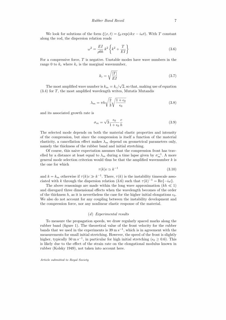
Figure 5. (i) Variation of the selected wavelength λm with the thickness of the rubberband h. The straight line stands for the theoretical curve with no adjusted parameters.(ii) Variation of the selected wavelength λm with the initial stretch ǫ0. The straight linestands for the theoretical curve from equation (3.8) with no adjusted factor. The curve fitis from equation (3.10) with τ(k)c = 2.6 k−1.

The measured value of V typically ranges from 4 m s−1 to 20 m s−1, dependingon the initial stretch (figure 4 (ii)). The evolution of the ratio V/c (c is the measuredfront speed) is in fair agreement with the theoretical prediction. Measurements ofthe stretching profile show that the front shape is well approximated by a stepfunction (figure 4 (i)). Actually, the dependency of V on initial stretch ǫ0 foundin section (b) is valid even for high initial stretching (ǫ0 ≃ 1), i.e. beyond thelimitations of the small strain hypothesis.

The first selected wavelength was obtained for rubber bands of thickness from0.254 mm up to 1.27 mm, for an initial stretch ǫ0 = 0.2 (figure 5 (i)). All propertiesand dimensions of the rubber bands are the same but their thickness. We find thatλm ∼ h as expected. Figure 5 (ii) shows the experimental wavelengths obtainedwith a rubber band of thickness h = 1.27 mm. Experimental results agree with theprediction from equation (3.8) for small initial stretching (i.e for high (1 + ǫ0)/ǫ0ratio). However for large initial stretch (i.e. for (1 + ǫ0)/ǫ0 smaller than 4) themeasured wavelengths are shorter than predicted from (3.8). A better fit is obtainedconsidering a mode selection criterion based on the length travelled by the re-compression front given in equation (3.10). For even higher initial stretch, (i.e. for(1 + ǫ0)/ǫ0 < 2), the wavelength becomes of the order of the band thickness andthe long wave approximation breaks down.

Note that using a dispersion relation that includes both Rayleigh’s correction(rotational inertia) and Timoshenko’s correction (effect of shear stress) leads to evenhigher wavelengths (see e.g. Graff, (1975)). Finaly, once the band is wrinkled, theaxial stress relaxes by a simple geometrical effect, as suggested by figure 1 (viii) and(ix)). This leads to a coarsening of the initial wrinkled pattern, a phenomenon whichis probably at the origin of Lindberg’s strong discrepancy between the anticipatedand measured wavelength.



4. Recoil of a rubber band in fluids

Several new effects are expected in the presence of an external fluid. First when theinstability develops, fluid must be moved together with the rod and thus we expectadded mass effects. Moreover, if the fluid is viscous, we expect damping. In thissection we modify the analysis of section 3 to account for these ingredients. As weshall see, in order to accurately describe the dynamic of the rubber band in a fluid,we must also consider the effect of viscosity on the axial stress front propagation.

(a) Modification of the instability

We consider a thin rod under compressive stress surrounded by an externalfluid. We use the same hypotheses and notations as in section 3 (b). The fluidis newtonian and incompressible, of density ρf and of kinematic viscosity ν. Thedispersion equation in non-dimensional form (see Appendix A) reads

(k∗ + 4M) σ2∗

+ 4χk∗

[

k∗ +

(

M

χσ∗ + k2

∗

)1/2]

σ∗ + 4 k3∗(k2

∗− 1) = 0 (4.1)

where k∗ = k/kc and σ∗ = σ/σm. M and χ are two non-dimensional numbersrelated to the added mass term and the viscous term, defined as

M =ρf

4πρkch, χ =

[

η2b

ρ|T |h

]1/2

(4.2)

where T = −Ebhǫ. χ depends on the dynamic viscosity η = ρfν of the fluid andon the Young modulus E, density ρ, thickness h and extensional strain of the rod(but b cancels out in the expression for χ when T is expressed in terms of E).

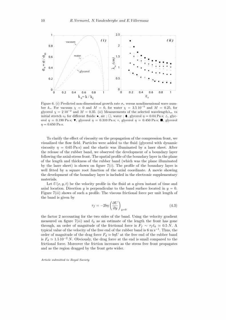
Figure 6 shows the dispersion relation obtained in different fluids (note that theglycerol we used was not pure and its dynamic viscosity was η = 0.65 Pa s). Theviscous number χ is rather small (χ = 0.02 for a dynamic viscosity η = 0.65 Pa s).Therefore, the main effect of the external fluid is the added mass effect that resultsin a significant decrease of the instability growth rate. Compared to the theoreticalvalue in vacuum, growth rate should decrease by a factor 1.6 for water and almost afactor 2 for glycerol. On the other hand, the selected wavelength is not significantlymodified by the interaction with the external fluid. For high χ numbers (i.e for highviscosity), the selected wave number decrease to an asymptotic value, k∗ m ∼ 1/

√3

instead of k∗ m = 1/√

2 with no external medium. The added mass tends to increasethe selected wavenumber anf for high values of M, k∗ m goes to

√

3/5.

(b) Experiments in fluids

We conducted experiments in water, and in water-glycerol mixtures with viscos-ity ranging from η = 4 10−3 Pa s up to η = 0.65 Pa s. Figure 6(ii) shows wavelengthsmeasured in air, water and water-glycerol mixtures. In water the results are similarto those performed in air. With more viscous fluids we observe a significant increaseof the selected wavelength. The wavelength is more than doubled in the glycerol(η = 0.65 Pa s). As discussed above, that effect is too large to be attributed to theimpact of viscosity on mode selection in the buckling instability.



0

0.2

0.4

0.6

0.8

1

0.2 0.4 0.6 0.8

σ ∗

k∗

vacuum

water

glycerol

0 1

= σ

/σm

= k / kc

0

0.5

1

1.5

2

2.5

0.2 0.4 0.6 0.8

λ m (c

m)

ε0

0 1

( i ) ( ii )

Figure 6. (i) Predicted non-dimensional growth rate σ∗ versus nondimensional wave num-ber k∗. For vacuum χ = 0 and M = 0, for water χ = 3.5 10−5 and M = 0.25, forglycerol χ = 2 10−2 and M = 0.35. (ii) Measurements of the selected wavelengthλm vsinitial stretch ǫ0 for different fluids: •, air ; �, water ; �, glycerol η = 0.04 Pa s; △, glyc-erol η = 0.190 Pa s; H, glycerol η = 0.310 Pa s; ◦, glycerol η = 0.450 Pa s; �, glycerolη = 0.650 Pa s.

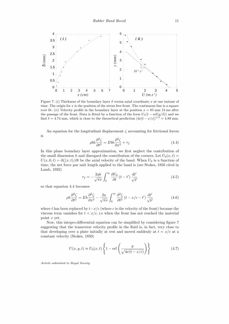
To clarify the effect of viscosity on the propagation of the compression front, wevisualized the flow field. Particles were added to the fluid (glycerol with dynamicviscosity η = 0.65 Pa s) and the elastic was illuminated by a laser sheet. Afterthe release of the rubber band, we observed the development of a boundary layerfollowing the axial-stress front. The spatial profile of the boundary layer in the planeof the length and thickness of the rubber band (which was the plane illuminatedby the laser sheet) is shown on figure 7(i). The profile of the boundary layer iswell fitted by a square root function of the axial coordinate. A movie showingthe development of the boundary layer is included in the electronic supplementarymaterials.

Let U(x, y, t) be the velocity profile in the fluid at a given instant of time andaxial location. Direction y is perpendicular to the band surface located in y = 0.Figure 7(ii) shows of such a profile. The viscous frictional force per unit length ofthe band is given by

τf = −2bη

(

∂U

∂y

)

y=0

(4.3)

the factor 2 accounting for the two sides of the band. Using the velocity gradientmeasured on figure 7(ii) and ℓ0 as an estimate of the length the front has gonethrough, an order of magnitude of the frictional force is Ff ∼ τf ℓ0 ≃ 0.5 N . Atypical value of the velocity of the free end of the rubber band is 6 m s−1. Thus, theorder of magnitude of the drag force Fd ≃ bηU at the free end of the rubber bandis Fd ≃ 1.5 10−2 N . Obviously, the drag force at the end is small compared to thefrictional force. Moreover the friction increases as the stress free front propagatesand as the region dragged by the front gets wider.



0

0.5

1

1.5

2

2.5

3

3.5

4

δ (m

m)

x (cm)0 1 2 3 4 5

U (m.s-1)

y (

mm

)

10 3 s-1

( i ) ( ii )

0 1 2 3 4 5 6 70

1

2

3

4

5

6

Figure 7. (i) Thickness of the boundary layer δ versus axial coordinate x at one instant oftime. The origin for x is the position of the stress free front. The continuous line is a squareroot fit. (ii) Velocity profile in the boundary layer at the position x = 85 mm 13 ms afterthe passage of the front. Data is fitted by a function of the form U0(1 − erf(y/δ)) and wefind δ = 4.74 mm, which is close to the theoretical prediction (4ν[t− x/c])1/2 = 4.89 mm.

An equation for the longitudinal displacement ζ accounting for frictional forcesis

ρbh∂2ζ

∂t2= Ebh

∂2ζ

∂x2+ τf (4.4)

In this plane boundary layer approximation, we first neglect the contribution ofthe small dimension h and disregard the contribution of the corners. Let U0(x, t) =U(x, 0, t) = ∂ζ(x, t)/∂t be the axial velocity of the band. When U0 is a function oftime, the net force par unit length applied to the band is (see Stokes, 1850 cited inLamb, 1932)

τf = − 2ηb√πν

∫

∞

0

∂U0

∂t(t − t′)

dt′√t′

(4.5)

so that equation 4.4 becomes

ρh∂2ζ

∂t2= Eh

∂2ζ

∂x2− 2η√

πν

∫

∞

0

∂2ζ

∂t2(t − x/c − t′)

dt′√t′

(4.6)

where t has been replaced by t−x/c (where c is the velocity of the front) because theviscous term vanishes for t < x/c, i.e when the front has not reached the materialpoint x yet.

Now, this integro-differential equation can be simplified by considering figure 7suggesting that the transverse velocity profile in the fluid is, in fact, very close tothat developing over a plate initially at rest and moved suddenly at t = x/c at aconstant velocity (Stokes, 1850)

U(x, y, t) ≈ U0(x, t)

{

1 − erf

(

y√

4ν(t − x/c)

)}

(4.7)



0.1

1

0.1

3/4

t / t0 1

0.1

1

0.1 1t*

3/4

( i ) ( ii )

5

10

15

20

25

15 20 25

ζ(c

m)

X (cm)

t = 5.25 mst = 8.75 ms

5 100

Figure 8. (i) Dimensionless width ∆/l versus dimensionless time t/t0. l is the length

of the stretched rubber band, t0 is the time such that Dt3/4

0= l2. ∆ is obtained by

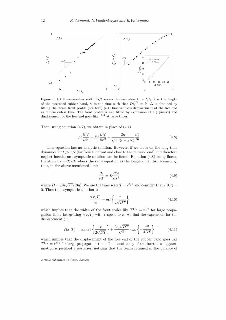
fitting the strain front profile (see text) (ii) Dimensionless displacement at the free endvs dimensionless time. The front profile is well fitted by expression (4.11) (insert) anddisplacement of the free end goes like t3/4 at large times.

Then, using equation (4.7), we obtain in place of (4.4)

ρh∂2ζ

∂t2= Eh

∂2ζ

∂x2− 2η√

πν(t − x/c)

∂ζ

∂t(4.8)

This equation has no analytic solution. However, if we focus on the long timedynamics for t ≫ x/c (far from the front and close to the released end) and thereforeneglect inertia, an asymptotic solution can be found. Equation (4.8) being linear,the stretch ǫ = ∂ζ/∂x obeys the same equation as the longitudinal displacement ζ,thus, in the above mentioned limit

∂ǫ

∂T= D

∂2ǫ

∂x2(4.9)

where D = Eh√

πν/(3η). We use the time scale T = t3/2 and consider that ǫ(0, t) =0. Then the asymptotic solution is

ǫ(x, T )

ǫ0= erf

{

x

2√

DT

}

(4.10)

which implies that the width of the front scales like T 1/2 = t3/4 for large propa-gation time. Integrating ǫ(x, T ) with respect to x, we find the expression for thedisplacement ζ :

ζ(x, T ) = ǫ0x erf

{

x

2√

DT

}

+2ǫ0

√DT√π

exp

{

− x2

4DT

}

(4.11)

which implies that the displacement of the free end of the rubber band goes likeT 1/2 = t3/4 for large propagation time. The consistency of the inertialess approx-imation is justified a posteriori noticing that the terms retained in the balance of



ε

x

ε0

0x

0

c

ε0

c

c

ε( i ) ( ii )

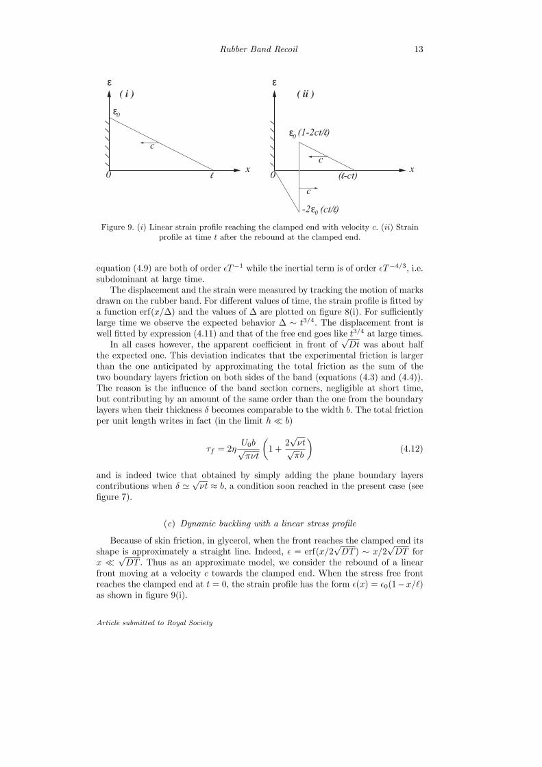
Figure 9. (i) Linear strain profile reaching the clamped end with velocity c. (ii) Strainprofile at time t after the rebound at the clamped end.

equation (4.9) are both of order ǫT−1 while the inertial term is of order ǫT−4/3, i.e.subdominant at large time.

The displacement and the strain were measured by tracking the motion of marksdrawn on the rubber band. For different values of time, the strain profile is fitted bya function erf(x/∆) and the values of ∆ are plotted on figure 8(i). For sufficientlylarge time we observe the expected behavior ∆ ∼ t3/4. The displacement front iswell fitted by expression (4.11) and that of the free end goes like t3/4 at large times.

In all cases however, the apparent coefficient in front of√

Dt was about halfthe expected one. This deviation indicates that the experimental friction is largerthan the one anticipated by approximating the total friction as the sum of thetwo boundary layers friction on both sides of the band (equations (4.3) and (4.4)).The reason is the influence of the band section corners, negligible at short time,but contributing by an amount of the same order than the one from the boundarylayers when their thickness δ becomes comparable to the width b. The total frictionper unit length writes in fact (in the limit h ≪ b)

τf = 2ηU0b√πνt

(

1 +2√

νt√πb

)

(4.12)

and is indeed twice that obtained by simply adding the plane boundary layerscontributions when δ ≃

√νt ≈ b, a condition soon reached in the present case (see

figure 7).

(c) Dynamic buckling with a linear stress profile

Because of skin friction, in glycerol, when the front reaches the clamped end itsshape is approximately a straight line. Indeed, ǫ = erf(x/2

√DT ) ∼ x/2

√DT for

x ≪√

DT . Thus as an approximate model, we consider the rebound of a linearfront moving at a velocity c towards the clamped end. When the stress free frontreaches the clamped end at t = 0, the strain profile has the form ǫ(x) = ǫ0(1−x/ℓ)as shown in figure 9(i).



0.1

1

10

-1/3

λ/λ

0

ε0.1 1

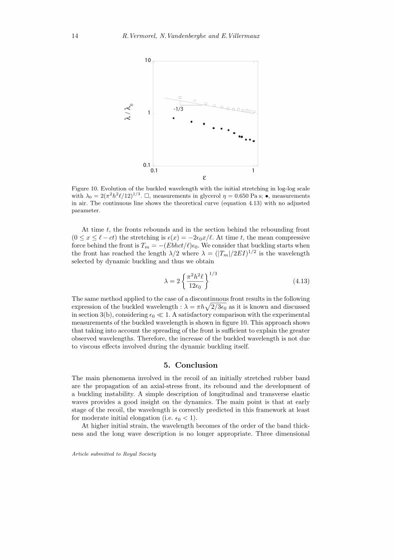
Figure 10. Evolution of the buckled wavelength with the initial stretching in log-log scalewith λ0 = 2(π2h2ℓ/12)1/3. �, measurements in glycerol η = 0.650 Pa s; •, measurementsin air. The continuous line shows the theoretical curve (equation 4.13) with no adjustedparameter.

At time t, the fronts rebounds and in the section behind the rebounding front(0 ≤ x ≤ ℓ− ct) the stretching is ǫ(x) = −2ǫ0x/ℓ. At time t, the mean compressiveforce behind the front is Tm = −(Ebhct/ℓ)ǫ0. We consider that buckling starts whenthe front has reached the length λ/2 where λ = (|Tm|/2EI)1/2 is the wavelengthselected by dynamic buckling and thus we obtain

λ = 2

{

π2h2ℓ

12ǫ0

}1/3

(4.13)

The same method applied to the case of a discontinuous front results in the followingexpression of the buckled wavelength : λ = πh

√

2/3ǫ0 as it is known and discussedin section 3(b), considering ǫ0 ≪ 1. A satisfactory comparison with the experimentalmeasurements of the buckled wavelength is shown in figure 10. This approach showsthat taking into account the spreading of the front is sufficient to explain the greaterobserved wavelengths. Therefore, the increase of the buckled wavelength is not dueto viscous effects involved during the dynamic buckling itself.

5. Conclusion

The main phenomena involved in the recoil of an initially stretched rubber bandare the propagation of an axial-stress front, its rebound and the development ofa buckling instability. A simple description of longitudinal and transverse elasticwaves provides a good insight on the dynamics. The main point is that at earlystage of the recoil, the wavelength is correctly predicted in this framework at leastfor moderate initial elongation (i.e. ǫ0 < 1).

At higher initial strain, the wavelength becomes of the order of the band thick-ness and the long wave description is no longer appropriate. Three dimensional



deformations lead to even smaller wavelength. Once the band is wrinkled, the axialstress relaxes by a simple geometrical effect leading to a coarsening of the initialundulations.

When the rubber band is immersed in a fluid, the major effect is the spreading ofthe initial front due to boundary layer friction. The smoother stress profile leads tolonger wavelength and a simple model based on a linear compressive strain profilegives a good estimate of the most amplified wavelength. Added mass effects slowdown the instability but do not modify mode selection appreciably. The impact ofboth fluid viscosity and density on the instability development are quantified withappropriate dimensionless numbers.

It was not necessary to account for a possible nonlinear elastic response of thematerial.

Appendix A. Dispersion relation for the buckling of a rod

interacting with a surrounding fluid

We derive the dispersion relation (equation 4.1) for the waves propagating alongthe rubber band in a viscous fluid, in two dimensions. In the reference (undeformed)state, the elastic rod is of infinite extent in the x direction and its thickness in they direction is h. There are two fluids domain, denoted by the index 1 for the upperpart (y > 0 in the reference configuration) and 2 for the lower part separated bythe rubber band. The model is based on the linearized Navier Stokes equation forthe two fluid domains.

ρ∂U1,2

∂t= −∂P1,2

∂x+ η

(

∂2U1,2

∂x2+

∂2U1,2

∂y2

)

(A 1)

ρ∂V1,2

∂t= −∂P1,2

∂y+ η

(

∂2V1,2

∂x2+

∂2V1,2

∂y2

)

(A 2)

The fluid is incompressible and thus, for the pressure, we have ∇2P1,2 = 0 and welook for P1 and P2 of the form

P1 = p(0)1 + p1 exp(−ky) exp(σt − ikx) (A 3)

P2 = p(0)2 + p1 exp(ky) exp(σt − ikx) (A 4)

where we have used the condition that P must remain finite at infinity. We lookfor V1,2 of the form :

V1,2 = v1,2(y) exp(σt − ikx) (A 5)

Using these forms for P1,2 and V1,2 in equations (A 1) and (A 2) we have

q2v1 −∂2v1

∂y2= −k

ηp1 exp(−ky) (A 6)

q2v2 −∂2v2

∂y2=

k

ηp2 exp(−ky) (A 7)

whereq2 =

ρσ

η+ k2 (A 8)



Thus for V1 and V2, we have (using the condition that V must remain finite)

V1 = {A1 exp(−qy) + B1 exp(−ky)} exp(σt − ikx) (A 9)

V2 = {A2 exp(qy) + B2 exp(ky)} exp(σt − ikx) (A 10)

with

p1 =η

k(q2 − k2)B1, and p2 =

η

k(q2 − k2)B2 (A 11)

We use the continuity equations

∂U1,2

∂x+

∂V1,2

∂y= 0 (A 12)

to obtain U1,2

U1,2 = − 1

ik

∂V1,2

∂y(A 13)

We need to specify the boundary conditions at the interface between the fluidand rod. There are four of them:

• Assuming that the cross sections of the rod are moving along the y directionwithout being stretched or compressed, the transverse displacement is there-fore homogenous along a section. Then we deduce the kinetic conditions atboth interfaces (y = ±h/2) in the transverse direction

V1|y=h/2 = V2|y=−h/2 =∂ξ

∂t(A 14)

• With a fluid initially at rest and in the slender slope limit, the difference ofhorizontal velocity across a section is

U1|y=h/2 − U2|y=−h/2 = −h∂2ξ

∂t∂x(A 15)

• Then, neglecting the thickness of the rod h versus the wavelength λ = 2π/k,the equation (A 15) leads to the kinetic condition in the axial direction

U1|y=h/2 = U2|y=−h/2 (A 16)

• Moreover, we are looking for modes that are anti-symmetrical across themedium line, i.e. such that

Γxy,1 = Γxy,2 (A 17)

where Γxy,1,2 is the xy term of the viscous stress tensor in the fluid. This con-dition also states that the shear stress at the rod surface is anti-symmetrical.

For the transverse motion of the rod, we use an Euler-Bernoulli model

ρ0S∂2ξ

∂t2+ EI

∂4ξ

∂x4+ T

∂2ξ

∂x2+ b∆

[

−P1,2 + n2 · (Γ1,2 n1,2)]

= 0 (A18)



where the last term of the left hand side represents the fluid-stress difference be-tween both sides of the rod. Γ is the viscous stress tensor in the fluid and n1,2 isthe vector normal to the interface. Γ in the fluid takes the form

Γ1,2

η∂U1,2

∂xη2

(

∂U1,2

∂y +∂V1,2

∂x

)

η2

(

∂U1,2

∂y +∂V1,2

∂x

)

η∂V1,2

∂y

(A 19)

At leading order, we have n1 = −n2 = (−∂ξ/∂x, 1) and thus,

∆[

n2 · (Γ1,2 n1,2)]

= 2η

(

∂V2

∂y

∣

∣

∣

y=h/2− ∂V1

∂y

∣

∣

∣

y=−h/2

)

(A 20)

Using these four conditions in equations A 6, A 7 and (A 14) we obtain a dispersionequation for the dynamic buckling of the rod in the fluid

A1 − A2 = (B2 − B1) exp

[

(q − k)h

2

]

(A 21)

Using the form of U1,2 (equation A 13) and (A 16) we obtain

A1 + A2 = −k

q(B2 + B1) exp

[

(q − k)h

2

]

(A 22)

And finally from the relation between tangential stress (equation A 17) and usingthe form of V (equations A 9 and A 10) and the form of U (equation A13), we get

A1 − A2 =2k2

q2 + k2(B2 − B1) exp

[

(q − k)h

2

]

(A 23)

Combining equations (A 21) and (A 23) and using equation (A 11), we have

A1 = A2 (A 24)

B1 = B2 (A 25)

p1 = −p2 (A 26)

Using equation (A 22) we find :

A1 = −k

qB1 exp

[

(q − k)h

2

]

(A 27)

We write ∆(−P1,2 + n2.(Γ1,2 n1,2)) in terms of B1 :

∆(−P1,2 + n2.(Γ1,2 n1,2))

={

(p1 − p2)e−

kh2 + ηq(A1 + A2)e

−qh

2 + ηk(B1 + B2)e−

kh2

}

eσt−ikx

=

{

2η(q2 − k2)

kB1e

−kh2

}

eσt−ikx (A 28)



The expression of ξ is obtained from the transversal boundary condition (equationA 14)

ξ =1

σ

{

A1e−

qh

2 + B1e−

kh2

}

eσt−ikx (A 29)

Introducing these expression in (A 18) and using the relation (A 21) we obtain thedispersion equation

(

ρ0S + 2ρb

k

)

σ2 + 2bη(k + q)σ + EIk4 − Tk2 = 0 (A 30)

In dimensionless form this relation reads

{k∗ + 4M}σ2∗

+ 4 χ k∗

{

k∗ +

(

M

χσ∗ + k2

∗

)1/2}

σ∗ + 4 k3∗(k2

∗− 1) = 0 (A 31)

with

k∗ =k

kc, σ∗ =

σ

σm(A 32)

The two dimensionless coefficients are

χ =

(

η2b

ρ0Th

)1/2

and M =ρλc

4πρ0h(A 33)

References

Bouasse, H. and Carriere, Z. 1903. Sur les courbes de traction du caoutchouc vulcanise.Annales de la faculte des sciences de Toulouse, 2e serie, 5, 257 - 283.

Euler, L. 1744. Addidentum I de curvis elasticis, methodus inveniendi lineas curvas maximiminimivi proprietate gaudentes. In Opera Omnia I, 231-297. Lausanne, 1744.

Gladden, J. R., Handzy, N.Z., Belmonte, A. and Villermaux, E. 2005. Dynamic bucklingand fragmentation in brittle rods. Phys. Rev. Lett., 94, 035503.

Graff, K. G. 1975. Wave motion in elastic solids. New York: Dover Publications.

Kolsky, H. 1949 . An investigation of the mechanical properties of materials at very highrates of loading. Proc. Phys. Soc. B, 62, 676-700.

Lamb, H. 1932. Hydrodynamics. Cambridge University Press.

Lindberg, H. E. 1965. Impact buckling of a bar. J. Appl. Mech., 32, 315-322.

Love, A. E. H. 1944. A treatise on the mathematical theory of elasticity. 4th edn. NewYork: Dover Publications.

Mullins, L. 1947. Effect of stretching on the properties of rubber. J. Rubber Res. 16,275-289.

Saint-Venant, M. and Flamant, A. 1883. Resistance vive ou dynamique des solides.Representtaion graphique des lois du choc longitudinal, subi a une des extremites parune tige ou barre prismatique assujettie a l’extremite opposee. C. R. Acad. Sci., 97,127-133.

Stokes, G. G. 1850 On the effect of the internal friction of fluids on the motion of pendu-lums. Trans. Camb. Phil. Soc., IX, 8, sec 52.


Documents

Rubber Band Recoil - HAL :: Accueil