RTG: A Recursive Realistic Graph Generator using …christos/PUBLICATIONS/pkdd09_rtg.pdfRTG: A Recursive Realistic Graph Generator using Random Typing 3 weighted graphs and by deﬁnition

RTG: A Recursive Realistic Graph Generatorusing Random Typing

Leman Akoglu Christos Faloutsos

Carnegie Mellon UniversitySchool of Computer Science

{lakoglu, christos}@cs.cmu.edu

Abstract. We propose a new, recursive model to generate realistic graphs,evolving over time. Our model has the following properties: it is (a) flex-ible, capable of generating the cross product of weighted/unweighted, di-rected/undirected, uni/bipartite graphs; (b) realistic, giving graphs thatobey eleven static and dynamic laws that real graphs follow (we formallyprove that for several of the (power) laws and we estimate their expo-nents as a function of the model parameters); (c) parsimonious, requiringonly four parameters. (d) fast, being linear on the number of edges; (e)simple, intuitively leading to the generation of macroscopic patterns. Weempirically show that our model mimics two real-world graphs very well:Blognet (unipartite, undirected, unweighted) with 27K nodes and 125Kedges; and Committee-to-Candidate campaign donations (bipartite, di-rected, weighted) with 23K nodes and 880K edges. We also show how tohandle time so that edge/weight additions are bursty and self-similar.

1 Introduction

Study of complex graphs such as computer and biological networks, the linkstructure of the WWW, the topology of the Internet, and recently with thewidespread use of the Internet, large social networks, has been a vital researcharea. Many fascinating properties have been discovered, such as small and shrink-ing diameter [2, 20], power-laws [5, 11, 16, 24, 22, 28, 29, 20], and community struc-tures [12, 13, 27]. As a result of such interesting patterns being discovered, andfor many other reasons which we will discuss next, how to find a model thatwould produce synthetic but realistic graphs is a natural question to ask. Thereare several applications and advantages of modeling real-world graphs:

– Simulation studies: if we want to run tests for, say a spam detection al-gorithm, and want to observe how the algorithm behaves on graphs withdifferent sizes and structural properties, we can use graph generators to pro-duce such graphs by changing the parameters. This is also true when it isdifficult to collect any kind of real data.

– Sampling/Extrapolation: we can generate a smaller graph for example forvisualization purposes or in case the original graph is too big to run testson it; or conversely to generate a larger graph for instance to make futureprediction and answer what-if questions.

2 Leman Akoglu Christos Faloutsos

– Summarization/Compression: model parameters can be used to summarizeand compress a given graph as well as to measure similarity to other graphs.

– Motivation to understand pattern generating processes: graph generators giveintuition and shed light upon what kind of processes can (or cannot) yield theemergence of certain patterns. Moreover, modeling addresses the question ofwhat patterns real networks exhibit that needs to be matched and providesmotivation to figure out such properties.

Graph generator models are surveyed in [4]. Ideally, we would like a graphgenerator that is:

1. simple: it would be easy to understand and it would intuitively lead to theemergence of macroscopic patterns.

2. realistic: it would produce graphs that obey all the discovered “laws” ofreal-world graphs with appropriate values.

3. parsimonious: it would require only a few number of parameters.4. flexible: it would be able to generate the cross product of weighted/unweighted,

directed/undirected and unipartite/bipartite graphs.5. fast: the generation process would ideally take linear time with respect to

the number of edges in the output graph.

In this paper we propose RTG, for Random Typing Generator. Our modeluses a process of ‘random typing’, to generate source- and destination- nodeidentifiers, and it meets all the above requirements. In fact, we show that it cangenerate graphs that obey all eleven patterns that real graphs typically exhibit.

Next, we provide a survey on related work. Section 3 describes our RTGgenerator in detail. Section 4 provides experimental results and discussion. Weconclude in Section 5. Appendix gives proofs showing some of the power-lawsthat the model generates.

2 Related Work

Graph patterns: Many interesting patterns that real graphs obey have beenfound, which we give a detailed list of in the next section. Ideally, a generatorshould be able to produce all of such properties.Graph generators: The vast majority of earlier graph generators have focusedon modeling a small number of common properties, but fail to mimic others.Such models include the Erdos & Renyi model [8], the preferential attachmentmodel [3] and numerous more, like the ‘small-world’, ‘winners don’t take all’,‘forest fire’ and ‘butterfly’ models [31, 26, 20, 22]. See [4] for a recent survey anddiscussion. In general, these methods are limited in trying to model some staticnetwork property while neglecting others as well as dynamic properties or cannotbe generalized to produce weighted graphs.

Random dot product graphs [17, 32] assign each vertex a random vector insome d-dimensional space and an edge is put between two vertices with proba-bility equal to the dot product of the endpoints. This model does not generate

RTG: A Recursive Realistic Graph Generator using Random Typing 3

weighted graphs and by definition only produces undirected graphs. It also seemsto require the computation of the dot product for each pair of nodes which takesquadratic time.

A different family of models is utility-based, where agents try to optimizea predefined utility function and the network structure takes shape from theircollective strategic behavior [10, 9, 18]. This class of models, however, is usuallyhard to analyze.

Kronecker graph generators [19] and their tensor followups [1] are successfulin the sense that they match several of the properties of real graphs and theyhave proved useful for generating self-similar properties of graphs. However, theyhave two disadvantages: The first is that they generate multinomial/lognormaldistributions for their degree and eigenvalue distribution, instead of a power-lawone. The second is that it is not easy to grow the graph incrementally: Theyhave a fixed, predetermined number of nodes (say, Nk, where N is the numberof nodes of the generator graph, and k is the number of iterations); where addingmore edges than expected does not create additional nodes. In contrast, in ourmodel, nodes emerge naturally.

3 Proposed Model

We first give a concise list of the static and dynamic ‘laws’ that real graphs obey,which a graph generator should be able to match.

L01 Power-law degree distribution: the degree distibution should follow a power-law in the form of f(d) ∝ dγ , with the exponent γ < 0 [5, 11, 16, 24]

L02 Densification Power Law (DPL): the number of nodes N and the numberof edges E should follow a power-law in the form of E(t) ∝ N(t)α, withα > 1, over time [20].

L03 Weigth Power Law (WPL): the total weight of the edges W and the numberof edges E should follow a power-law in the form of W (t) ∝ E(t)β , withβ > 1, over time [22].

L04 Snapshot Power Law (SPL): the total weight of the edges Wn attached toeach node and the number of such edges, that is, the degree dn should followa power-law in the form of Wn ∝ dθ

n, with θ > 1 [22].L05 Triangle Power Law (TPL): the number of triangles ∆ and the number of

nodes that participate in ∆ number of triangles should follow a power-lawin the form of f(∆) ∝ ∆σ, with σ < 0 [29].

L06 Eigenvalue Power Law (EPL): the eigenvalues of the adjacency matrix ofthe graph should be power-law distributed [28].

L07 Principal Eigenvalue Power Law (λ1PL): the largest eigenvalue λ1 of theadjacency matrix of the graph and the number of edges E should follow apower-law in the form of λ1(t) ∝ E(t)δ, with δ < 0.5, over time [1].

L08 small and shrinking diameter: the (effective) diameter of the graph shouldbe small [2] with a possible spike at the ‘gelling point’ [22]. It should alsoshrink over time [20].


L09 constant size secondary and tertiary connected components: while the ‘giantconnected component’ keeps growing, the secondary and tertiary connectedcomponents tend to remain constant in size with small oscillations [22].

L10 community structure: the graph should exhibit a modular structure, withnodes forming groups, and possibly groups within groups [12, 13, 27].

L11 bursty/self-similar edge/weight additions: Edge (weight) additions to thegraph over time should be self-similar amd bursty rather than uniform withpossible spikes [7, 14, 15, 22].

Zipf introduced probably the earliest power law [33], stating that, in manynatural languages, the rank r and the frequency fr of vocabulary words followa power-law fr ∝ 1/r. Mandelbrot [21] argued that Zipf‘s law is the resultof optimizing the average amount of information per unit transmission cost.Miller [23] showed that a random process also leads to Zipf-like power laws. Hesuggested the following experiment: “A monkey types randomly on a keyboardwith k characters and a space bar. A space is hit with probability q; all othercharacters are hit with equal probability, (1−q)

k . A space is used to separatewords”. The resulting words of this random typing process follow a power-law.Conrad and Mitzenmacher [6] showed that this relation still holds when the keysare hit with unequal probability.

Our model generalizes the above model of natural human behavior, using‘random typing’. We build our model RTG (Random Typing Generator) in threesteps, incrementally. In the next two steps, we introduce the base version of theproposed model to give an insight. However, as will become clear, it has twoshortcomings in matching desired real-world properties. In particular, the basemodel does not capture (1) homophily, and (2) community structure.

3.1 RTG-IE: RTG with Independent Equiprobable keys

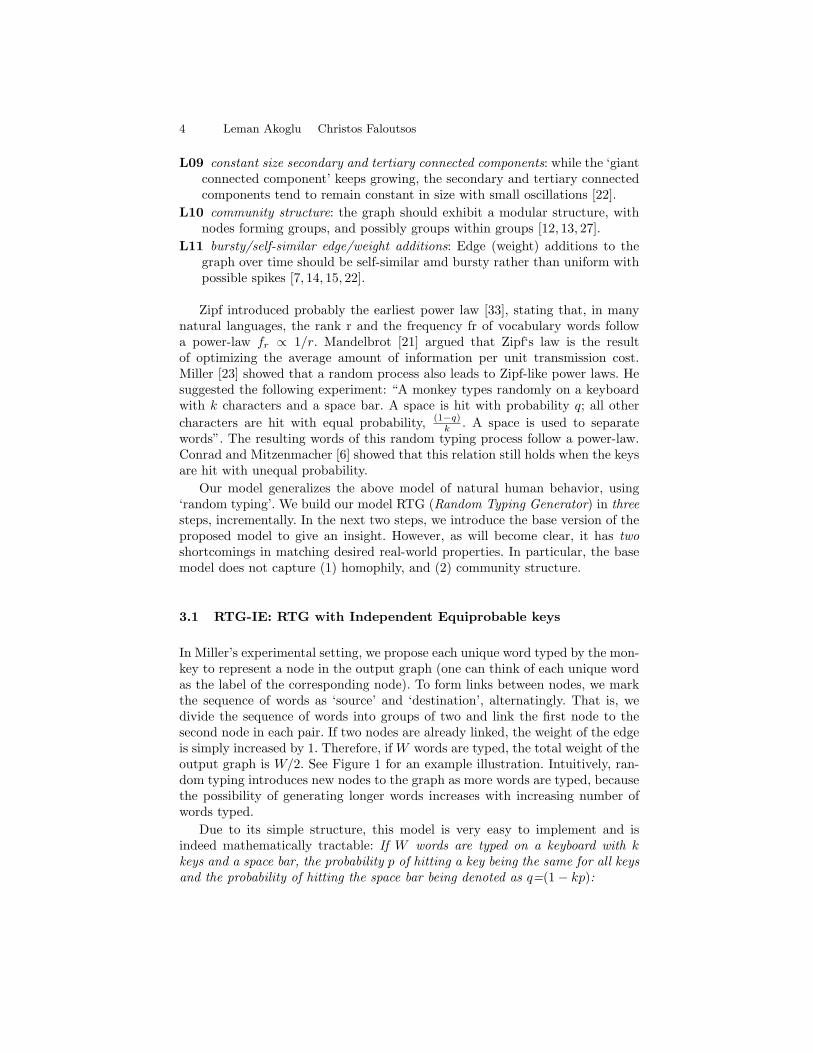
In Miller’s experimental setting, we propose each unique word typed by the mon-key to represent a node in the output graph (one can think of each unique wordas the label of the corresponding node). To form links between nodes, we markthe sequence of words as ‘source’ and ‘destination’, alternatingly. That is, wedivide the sequence of words into groups of two and link the first node to thesecond node in each pair. If two nodes are already linked, the weight of the edgeis simply increased by 1. Therefore, if W words are typed, the total weight of theoutput graph is W/2. See Figure 1 for an example illustration. Intuitively, ran-dom typing introduces new nodes to the graph as more words are typed, becausethe possibility of generating longer words increases with increasing number ofwords typed.

Due to its simple structure, this model is very easy to implement and isindeed mathematically tractable: If W words are typed on a keyboard with kkeys and a space bar, the probability p of hitting a key being the same for all keysand the probability of hitting the space bar being denoted as q=(1− kp):


Time Source Destination Weight

T1 ab a 1

T2 bba ab 1

T3 b ab 1

T4 a b 1

T5 ab a 1… … … …

a b S

a ab b SS

p qp

p p qq

q

p p

pp

ab a bba ab b ab a b ab a

Fig. 1. Illustration of the RTG-IE. Upper left: how words are (recursively) generatedon a keyboard with two equiprobable keys, ‘a’ and ‘b’, and a space bar; lower left:a keyboard is used to randomly type words, separated by the space character; upperright: how words are organized in pairs to create source and destination nodes in thegraph over time; lower right: the output graph; each node label corresponds to a uniqueword, while labels on edges denote weights.

Lemma 1. The expected number of nodes N in the output graph G of the RTG-IE model is

N ∝ W−logpk.

Proof: In the Appendix. ut

Lemma 2. The expected number of edges E in the output graph G of the RTG-IE model is

E ≈ W−logpk ∗ (1 + c′logW ), for c′ =q−logpk

−logp> 0.

Proof: In the Appendix. ut

Lemma 3. The in(out)-degree dn of a node in the output graph G of the RTG-IE model is power law related to its total in(out)-weight Wn, that is,

Wn ∝ d−logkpn

with expected exponent −logkp > 1.

Proof: In the Appendix. utEven though most of the properties listed at the beginning of this section are

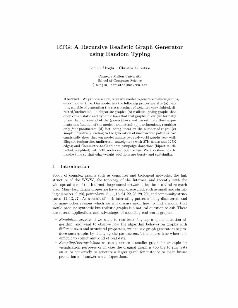
matched, there are two problems with this model: (1) the degree distributionfollows a power-law only for small degrees and then shows multinomial charac-teristics (See Figure 2), and (2) it does not generate homophily and communitystructure, because it is possible for every node to get connected to every othernode, rather than to ‘similar’ nodes in the graph.


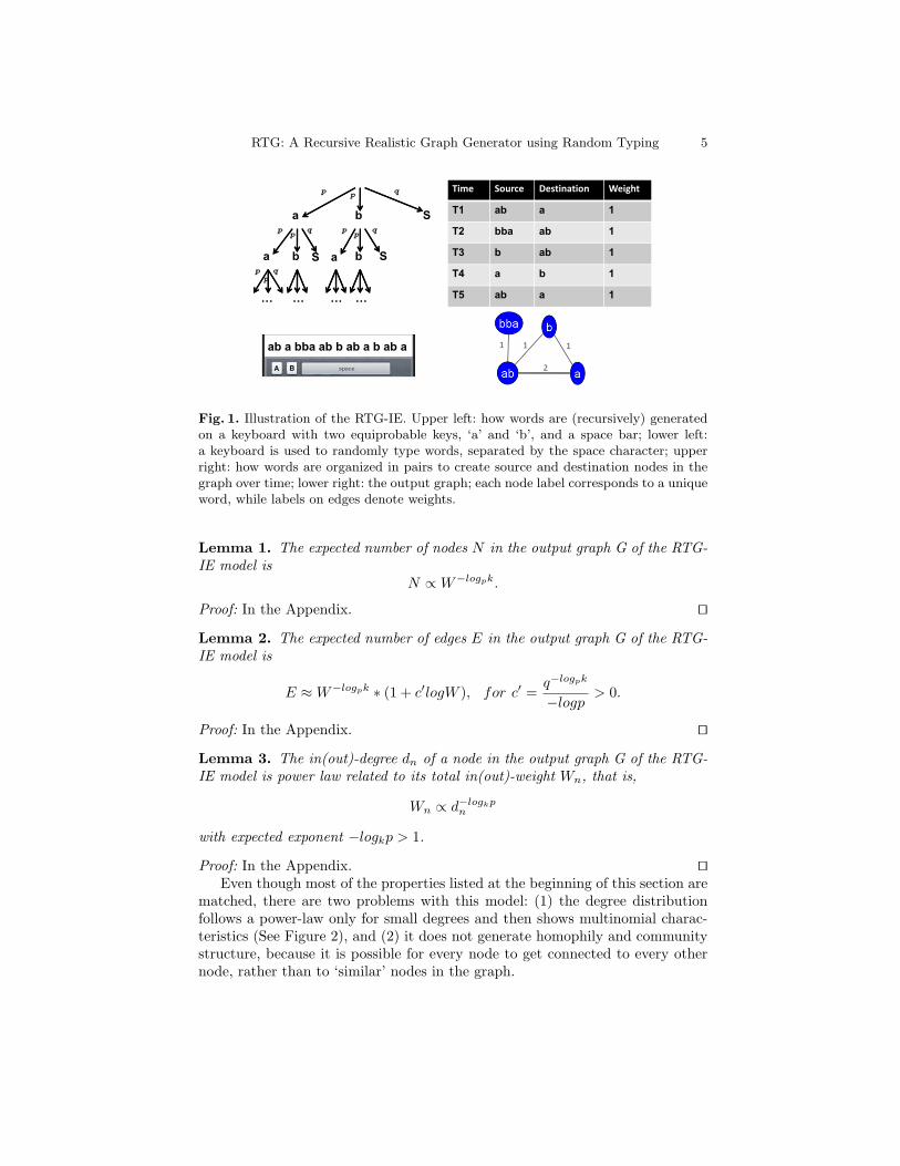
Fig. 2. Top row: Results of RTG-IE (k = 5, p = 0.16, W = 1M). The problem withthis model is that in(out)-degrees form multinomial clusters (left). This is becausenodes with labels of the same length are expected to have the same degree. This canbe observed on the rank-frequency plot (right) where we see many words with thesame frequency. Notice the ‘staircase effect’. Bottom row: Results of RTG-IU (k = 5,p = [0.03, 0.05, 0.1, 0.22, 0.30], W = 1M). Unequal probabilities introduce smoothingon the frequency of words that are of the same length (right). As a result, the degreedistribution follows a power-law with expected heavy tails (left).

3.2 RTG-IU: RTG with Independent Un-equiprobable keys

We can spread the degrees so that nodes with the same-length but otherwisedistinct labels would have different degrees by making keys have unequal prob-abilities. This procedure introduces smoothing in the distribution of degrees,which remedies the first problem introduced by the RTG-IE model. In addition,thanks to [6], we are still guaranteed to obtain the desired power-law character-istics as before. See Figure 2.

3.3 RTG: Random Typing Graphs

What the previous model fails to capture is the homophily and community struc-ture. In a real network, we would expect nodes to get connected to similar nodes(homophily), and form groups and possibly groups within groups (modular struc-ture). In our model, for example on a keyboard with two keys ‘a’ and ‘b’, wewould like nodes with many ‘a’s in their labels to be connected to similar nodes,as opposed to nodes labeled with many ‘b’s. However, in both RTG-IE and


RTG-IU it is possible for every node to conenct to every other node. In fact, thisyields a tightly connected core of nodes with rather short labels.

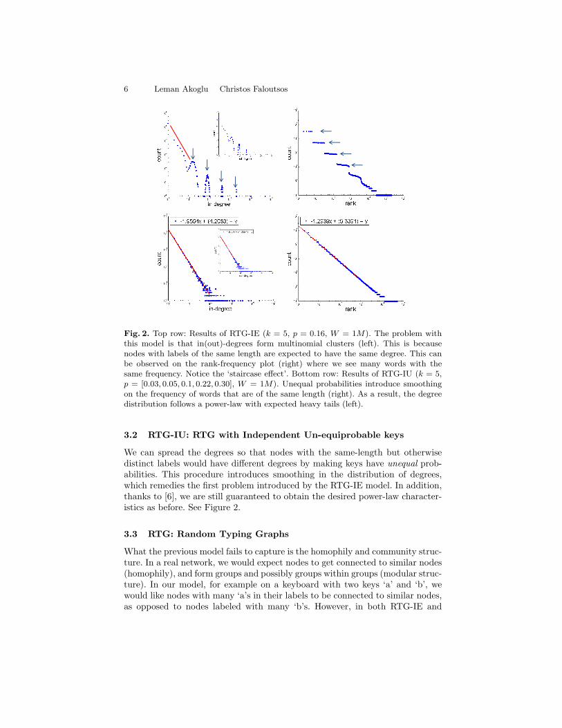
Our proposal to fix this is to envision a two-dimensional keyboard that gener-ates source and destination labels in one shot, as shown in Figure 3. The previousmodel generates a word for source, and, completely independently, another wordfor destination. In the example with two keys, we can envision this process aspicking one of the nine keys in Figure 3(a), using the independence assumption:the probability for each key is the product of the probability of the correspond-ing row times the probability of the corresponding column: pl for letter l, andq for space (‘S’). After a key is selected, its row character is appended to thesource label, and the column character to the destination label. This processrepeats recursively as in Figure 3(b), until the space character is hit on the firstdimension in which case the source label is terminated and also on the seconddimension in which case the destination label is terminated.

a

b b*

ab*-aa*

aS-aa*

a b S

a

b b*- b*b*- a*

a*- b*

b*- S

a*- Sa*- a*

b

S

b*

S

b

S

b*- b*b*- a* b*- S

S - a* S - b* S - S

a b S

b*- b*b*- a*

a*- b*

b*- S

a*- S

aS-aSaS-ab*

aa*-aSaa*-

ab*

ab*-aSab*-

ab*

a b

a

b

pap

prob(a*,a*) =

pa – prob(a*,b*)

– prob(a*,S)

pbpaβprob(b*,

pb – prob(b*,

– prob(b*,S) b*- b*b*- a* b*- S

S - a* S - b* S - S

b

S qpqpaβ

pbpaβ b

– prob(b*,S)

pa p

a b S

a

b b*- b*b*- a*

a*- b*

b*-

a*-

aS-aS

ab*-aa*

aS-aa* aS-ab*

aa*-aSaa*-

ab*

ab*-aSab*-

ab*

b S

b*- b*

a*- b*

b*- S

a*- S

b

S

b*- b*b*- a* b*-

S - a* S - b* S -

b*- b* b*- S

S - b* S - S

S

- S

- S

a b S

a

b

papbβ

prob(a*,a*) =

pa – prob(a*,b*)

– prob(a*,S)

pbqβpbpaβ

paqβ

prob(b*,b*) =

pb – prob(b*,a*)

– prob(b*,S)

pa

pb- S

- S

b

S

pbqβ

qpbβqpaβ

pbpaβ b

– prob(b*,S)

prob(S,S) =

q – prob(S,a*)

– prob(S,b*)

pb

q

pa pb q

(a) first level (b) recursion (c) communities

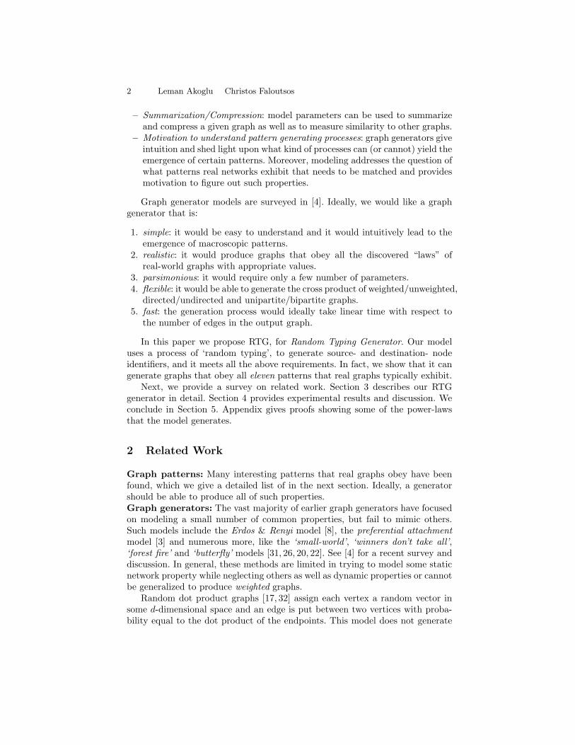
Fig. 3. The RTG model: random typing on a 2-d keyboard, generating edges (source-destination pairs). See Algorithm 1. (a) an example 2-d keyboard (nine keys), hitting akey generates the row(column) character for source(destination), shaded keys terminatesource and/or destination words. (b) illustarates recursive nature. (c) the imbalancefactor β favors diagonal keys and leads to homophily.

In order to model homophily and communities, rather than assigning cross-product probabilities to keys on the 2-d keyboard, we introduce an imbalancefactor β, which will decrease the chance of a-to-b edges, and increase the chancefor a-to-a and b-to-b edges, as shown in Figure 3(c). Thus, for the example thatwe have, the formulas for the probabilities of the nine keys become:

prob(a, b) = papbβ prob(a, S) = paqβ prob(a, a) = pa − (prob(a, b) + prob(a, S))prob(b, a) = pbpaβ prob(b, S) = pbqβ prob(b, b) = pb − (prob(b, a) + prob(b, S))prob(S, a) = qpaβ prob(S, b) = qpbβ prob(S, S) = q − (prob(S, a) + prob(S, b))

By boosting the probabilities of the diagonal keys and downrating the probabil-ities of the off-diagonal keys, we are guaranteed that nodes with similar labelswill have higher chance to get connected. The pseudo-code of generating edgesas described above is shown in Algorithm 1.


Next, before showing the experimental results of RTG, we take a detour todescribe how we handle time so that edge/weight additions are bursty and self-similar. We also discuss the generalizations of the model in order to produce alltypes of uni/bipartite, (un)weighted, and (un)directed graphs.

Algorithm 1 RTGInput: k, q, W , βOutput: edge-list L for output graph G1: Initialize (k + 1)-by-(k + 1) matrix M with cross-product probabilities2: // in order to ensure homophily and community structure3: Multiply off-diagonal probabilities by β, 0 < β < 14: Boost diagonal probabilities such that sum of row(column) probabilities remain

the same.5: Initialize edge list L6: for 1 to W do7: L1, L2 ← SelectNodeLabels(M)8: Append L1, L2 to L9: end for

10:11: function SelectNodeLabels (M) : L1, L212: Initialize L1 and L2 to empty string13: while not terminated L1 and not terminated L2 do14: Pick a random number r, 0 < r < 115: if r falls into M(i, j), i ≤ k, j ≤ k then16: Append character ‘i’ to L1 and ‘j’ to L2 if not terminated17: else if r falls into M(i, j), i ≤ k, j=k + 1 then18: Append character ‘i’ to L1 if not terminated19: Terminate L220: else if r falls into M(i, j), i=k + 1, j ≤ k then21: Append character ‘j’ to L2 if not terminated22: Terminate L123: else24: Terminate L1 and L225: end if26: end while27: Return L1 and L228: end function

3.4 Burstiness and Self-similarity

Most real-world traffic as well as edge/weight additions to real-world graphshave been found to be self-similar and bursty [7, 14, 15, 22]. Therefore, in thissection we give a brief overview of how to aggregate time so that edge andweight additions, that is ∆E and ∆W, are bursty and self-similar.

Notice that when we link two nodes at each step, we add 1 to the total weightW . So, if every step is represented as a single time-tick, the weight additions are


uniform. However, to generate bursty traffic, we need to have a bias factor b> 0.5,such that b-fraction of the additions happen in one half and the remaining in theother half. We will use the b-model [30], which generates such self-similar andbursty traffic. Specifically, starting with a uniform interval, we will recursivelysubdivide weight additions to each half, quarter, and so on, according to thebias b. To create randomness, at each step we will randomly swap the order offractions b and (1− b).

Among many methods that measure self-similarity we use the entropy plot [30],which plots the entropy H(r) versus the resolution r. The resolution is the scale,that is, at resolution r, we divide our time interval into 2r equal sub-intervals,compute ∆E in each sub-interval k(k = 1 . . . 2r), normalize into fractions pk =∆EE , and compute the Shannon entropy H(r) of the sequence pk. If the plot H(r)

is linear, the corresponding time sequence is said to be self-similar, and the slopeof the plot is defined as the fractal dimension fd of the time sequence. Noticethat a uniform ∆ distribution yields fd=1; a lower value of fd corresponds toa more bursty time sequence, with a single burst having the lowest fd=0: thefractal dimension of a point.

3.5 Generalizations

We can easily generalize RTG to model all type of graphs. To generate undirectedgraphs, we can simply assume edges from source to destination to be undirectedas the formation of source and destination labels is the same and symmetric.For unweighted graphs, we can simply ignore duplicate edges, that is, edgesthat connect already linked nodes. Finally, for bipartite graphs, we can use twodifferent sets of keys such that on the 2-d keyboard, source dimension containskeys from the first set, and the destination dimension from the other set. Thisassures source and destination labels to be completely different, as desired.

4 Experimental Results

The question we wish to answer here is how RTG is able to model real-worldgraphs. The datasets we used are:Blognet: a social network of blogs based on citations (undirected, unipartite andunweighted with N=27, 726; E=126, 227; over 80 time ticks).Com2Cand: the U.S. electoral campaign donations network from organizationsto candidates (directed, bipartite and weighted with N=23, 191; E=877, 721;and W=4, 383, 105, 580 over 29 time ticks). Weights on edges indicate donateddollar amounts.

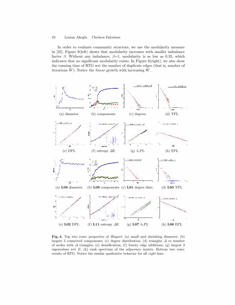
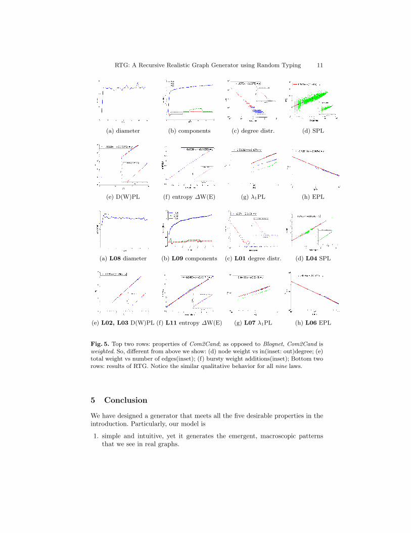
In Figures 4 and 5, we show the related patterns for Blognet and Com2Candas well as synthetic results, respectively. In order to model these networks, weran experiments for different parameter values k, q, W , and β. Here, we show theclosest results that RTG generated, though fitting the parameters is a challengingfuture direction. We observe that RTG is able match the long wish-list of staticand dynamic properties for the two real graphs.


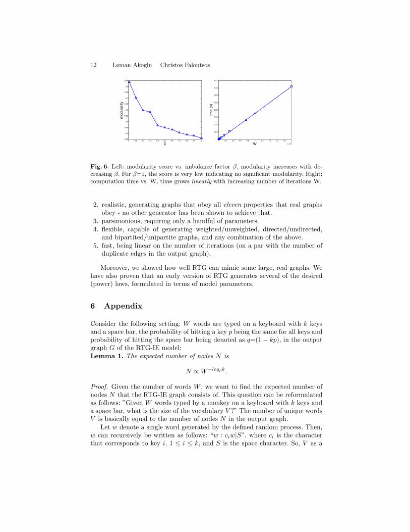
In order to evaluate community structure, we use the modularity measurein [25]. Figure 6(left) shows that modularity increases with smaller imbalancefactor β. Without any imbalance, β=1, modularity is as low as 0.35, whichindicates that no significant modularity exists. In Figure 6(right), we also showthe running time of RTG wrt the number of duplicate edges (that is, number ofiterations W ). Notice the linear growth with increasing W .

(a) diameter (b) components (c) degrees (d) TPL

(e) DPL (f) entropy ∆E (g) λ1PL (h) EPL

(a) L08 diameter (b) L09 components (c) L01 degree distr. (d) L05 TPL

(e) L02 DPL (f) L11 entropy ∆E (g) L07 λ1PL (h) L06 EPL

Fig. 4. Top two rows: properties of Blognet: (a) small and shrinking diameter; (b)largest 3 connected components; (c) degree distribution; (d) triangles ∆ vs numberof nodes with ∆ triangles; (e) densification; (f) bursty edge additions; (g) largest 3eigenvalues wrt E; (h) rank spectrum of the adjacency matrix. Bottom two rows:results of RTG. Notice the similar qualitative behavior for all eight laws.


(a) diameter (b) components (c) degree distr. (d) SPL

(e) D(W)PL (f) entropy ∆W(E) (g) λ1PL (h) EPL

(a) L08 diameter (b) L09 components (c) L01 degree distr. (d) L04 SPL

(e) L02, L03 D(W)PL (f) L11 entropy ∆W(E) (g) L07 λ1PL (h) L06 EPL

Fig. 5. Top two rows: properties of Com2Cand; as opposed to Blognet, Com2Cand isweighted. So, different from above we show: (d) node weight vs in(inset: out)degree; (e)total weight vs number of edges(inset); (f) bursty weight additions(inset); Bottom tworows: results of RTG. Notice the similar qualitative behavior for all nine laws.

5 Conclusion

We have designed a generator that meets all the five desirable properties in theintroduction. Particularly, our model is

1. simple and intuitive, yet it generates the emergent, macroscopic patternsthat we see in real graphs.


0 0.1 0.2 0.3 0.4 0.5 0.6 0.7 0.8 0.9 10.35

0.4

0.45

0.5

0.55

0.6

0.65

0.7

0.75

0.8

0.85

β

mod

ular

ity

0 0.2 0.4 0.6 0.8 1 1.2 1.4 1.6 1.8 2

x 106

0

1000

2000

3000

4000

5000

6000

7000

8000

W

time

(s)

Fig. 6. Left: modularity score vs. imbalance factor β, modularity increases with de-creasing β. For β=1, the score is very low indicating no significant modularity. Right:computation time vs. W, time grows linearly with increasing number of iterations W.

2. realistic, generating graphs that obey all eleven properties that real graphsobey - no other generator has been shown to achieve that.

3. parsimonious, requiring only a handful of parameters.4. flexible, capable of generating weighted/unweighted, directed/undirected,

and bipartited/unipartite graphs, and any combination of the above.5. fast, being linear on the number of iterations (on a par with the number of

duplicate edges in the output graph).

Moreover, we showed how well RTG can mimic some large, real graphs. Wehave also proven that an early version of RTG generates several of the desired(power) laws, formulated in terms of model parameters.

6 Appendix

Consider the following setting: W words are typed on a keyboard with k keysand a space bar, the probability of hitting a key p being the same for all keys andprobability of hitting the space bar being denoted as q=(1− kp), in the outputgraph G of the RTG-IE model:Lemma 1. The expected number of nodes N is

N ∝ W−logpk.

Proof. Given the number of words W , we want to find the expected number ofnodes N that the RTG-IE graph consists of. This question can be reformulatedas follows: ”Given W words typed by a monkey on a keyboard with k keys anda space bar, what is the size of the vocabulary V ?” The number of unique wordsV is basically equal to the number of nodes N in the output graph.

Let w denote a single word generated by the defined random process. Then,w can recursively be written as follows: “w : ciw|S”, where ci is the characterthat corresponds to key i, 1 ≤ i ≤ k, and S is the space character. So, V as a


function of model parameters can be formulated as:

V (W ) = V (c1,Wp) + V (c2,Wp) + . . . + V (ck,Wp) + V (S)

= k ∗ V (Wp) + V (S) = k ∗ V (Wp) +{ 1, 1− (1− q)W

0, (1− q)W

where q denotes the probability of hitting the space bar, i.e. q = 1 − kp. Giventhe fact that W is often large, and (1− q) < 1, it is almost always the case thatw=S is generated; but since this adds only a constant factor, we can ignore itin the rest of the computation. That is,

V (W ) ≈ k ∗ V (Wp) = k ∗ (k ∗ V (Wp2)) = kn ∗ V (1)

where n = logp(1/W ) = −logpW . By definition, when W=1, that is, in caseonly one word is generated, the vocabulary size is 1, i.e. V(1)=1. Therefore,

V (W ) = N ∝ kn = k−logpW = W−logpk.ut

100

101

102

103

104

105

106

10−1

100

101

102

103

104

105

106

W [1

:1M

]

E = Wlogpk*(1+c’logW)

1.2131x + (−0.40331) = y

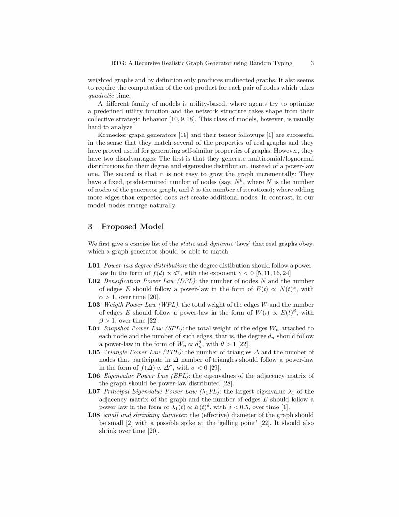
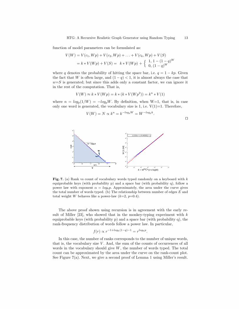
Fig. 7. (a) Rank vs count of vocabulary words typed randomly on a keyboard with kequiprobable keys (with probability p) and a space bar (with probability q), follow apower law with exponent α = logkp. Approximately, the area under the curve givesthe total number of words typed. (b) The relationship between number of edges E andtotal weight W behaves like a power-law (k=2, p=0.4).

The above proof shown using recursion is in agreement with the early re-sult of Miller [23], who showed that in the monkey-typing experiment with kequiprobable keys (with probability p) and a space bar (with probability q), therank-frequency distribution of words follow a power law. In particular,

f(r) ∝ r−1+logk(1−q)−1 = rlogkp.

In this case, the number of ranks corresponds to the number of unique words,that is, the vocabulary size V . And, the sum of the counts of occurrences of allwords in the vocabulary should give W , the number of words typed. The totalcount can be approximated by the area under the curve on the rank-count plot.See Figure 7(a). Next, we give a second proof of Lemma 1 using Miller’s result.


Proof. Let α = logkp and C(r) denote the number of times that the word withrank r is typed. Then, C(r) = crα, where C(r)min = C(V ) = cV α and theconstant c = C(V )V −α. Then we can write W as

W = C(V )V −α

(V∑

r=1

rα

)≈ C(V )V −α

(∫ V

r=1

rαdr

)= C(V )V −α

(rα+1

α + 1

∣∣∣Vr=1

)= C(V )V −α

(1

−α− 1− 1

(−α− 1)V −α−1

)≈ c′V −α.

where c′ = C(V )−α−1 , where α < −1 and C(V ) is very small (usually 1). Therefore,

V = N ∝ W− 1α = W−logpk.

utLemma 2. The expected number of edges E is

E ≈ W−logpk ∗ (1 + c′logW ), for c′ =q−logpk

−logp> 0.

Proof. Given the number of words W , we want to find the expected number ofedges E that the RTG-IE graph consists of. The number of edges E is the sameas the unique number of pairs of words. We can think of a pair of words as asingle word e, the generation of which is stopped after the second hit to the spacebar. So, e always contains a single space character. Recursively, “e : cie|Sw”,where “w : ciw|S”. So, E can be formulated as:

E(W ) = k ∗ E(Wp) + V (Wq) (1)

V (Wq) = k ∗ V (Wqp) +{ 1, 1− (1− q)Wq

0, (1− q)Wq (2)

From Lemma 1, Equ.(2) can be approximately written as V (Wq) = (Wq)−logpk.Then, Equ.(1) becomes E(W ) = k ∗ E(Wp) + cWα, where c = q−logpk andα = −logpk. Given that E(W=1)=1, we can solve the recursion as follows:

E(W ) ≈ k ∗ (k ∗ E(Wp2) + c(Wp)α) + cWα

= k ∗ (k ∗ (k ∗ V (Wp3) + c(Wp2)α) + c(Wp)α) + cWα

= kn ∗ V (1) + kn−1 ∗ c(Wpn−1) + kn−2 ∗ c(Wpn−2)α + . . . + cWα

= kn ∗ V (1) + cWα((kpα)n−1 + (kpα)n−2 + . . . + 1)

where n = logp(1/W ) = −logpW . Since kpα = kp−logpk = 1,

E(W ) ≈ kn ∗ V (1) + n ∗ cWα = k−logpW + c−log 1

W

−logpW−logpk = W−logpk(1 + c′logW )

where c′ = c−logp = q−logpk

−logp > 0.


utThe above function of E in terms of W and other model parameters looks likea power-law for a wide range of W . See Figure 7(b).Lemma 3. The in/out-degree dn of a node is power law related to its totalin/out-weight Wn, that is,

Wn ∝ d−logkpn

with expected exponent −logkp > 1.

Proof. We will show that Wn ∝ d−logkpn for out-edges, and a similar argument

holds for in-edges. Given that the experiment is repeated W times, let Wn denotethe number of times a unique word is typed as a source. Each such unique wordcorresponds to a node in the final graph and Wn is basically its out-weight, sincethe node appears as a source node. Then, the out-degree dn of a node is simplythe number of unique words typed as a destination. From Lemma 1,

Wn ∝ d−logkpn , for − logkp > 1.

utAcknowledgmentsThis material is based upon work supported by the National Science Foundation under Grants No.IIS-0705359 and CNS-0721736. This work is also partially supported by an IBM Faculty Award, aYahoo Research Alliance Gift, a SPRINT gift, with additional funding from Intel, NTT and Hewlett-Packard. Any opinions, findings, and conclusions or recommendations expressed in this material arethose of the author(s) and do not necessarily reflect the views of any of the funding parties.

References

1. L. Akoglu, M. McGlohon, and C. Faloutsos. Rtm: Laws and a recursive generatorfor weighted time-evolving graphs. In ICDM, 2008.

2. R. Albert, H. Jeong, and A.-L. Barabasi. Diameter of the World Wide Web.Nature, 401:130–131, 1999.

3. A. L. Barabasi and R. Albert. Emergence of scaling in random networks. Science,286(5439):509–512, October 1999.

4. D. Chakrabarti and C. Faloutsos. Graph mining: Laws, generators, and algorithms.ACM Comput. Surv., 38(1), 2006.

5. D. Chakrabarti, Y. Zhan, and C. Faloutsos. R-MAT: A recursive model for graphmining. SIAM Int. Conf. on Data Mining, Apr. 2004.

6. B. Conrad and M. Mitzenmacher. Power laws for monkeys typing randomly:the case of unequal probabilities. IEEE Transactions on Information Theory,50(7):1403–1414, 2004.

7. M. Crovella and A. Bestavros. Self-similarity in world wide web traffic, evidenceand possible causes. Sigmetrics, pages 160–169, 1996.

8. P. Erdos and A. Renyi. On the evolution of random graphs. Publ. Math. Inst.Hungary. Acad. Sci., 5:17–61, 1960.

9. E. Even-Bar, M. Kearns, and S. Suri. A network formation game for bipartiteexchange economies. In SODA, 2007.

10. A. Fabrikant, A. Luthra, E. N. Maneva, C. H. Papadimitriou, and S. Shenker. Ona network creation game. In PODC, 2003.

11. M. Faloutsos, P. Faloutsos, and C. Faloutsos. On power-law relationships of theinternet topology. SIGCOMM, pages 251–262, Aug-Sept. 1999.


12. G. W. Flake, S. Lawrence, C. L. Giles, and F. M. Coetzee. Self-organization andidentification of web communities. IEEE Computer, 35:66–71, 2002.

13. M. Girvan and M. E. J. Newman. Community structure in social and biologicalnetworks. PNAS, 99:7821, 2002.

14. M. E. Gomez and V. Santonja. Self-similarity in i/o workload: Analysis and mod-eling. In WWC, 1998.

15. S. D. Gribble, G. S. Manku, D. Roselli, E. A. Brewer, T. J. Gibson, and E. L.Miller. Self-similarity in file systems. In SIGMETRICS ’98, 1998.

16. J. M. Kleinberg, R. Kumar, P. Raghavan, S. Rajagopalan, and A. S. Tomkins. TheWeb as a graph: Measurements, models and methods. Lecture Notes in ComputerScience, 1627:1–17, 1999.

17. S. E. Kraetzl M., Nickel C. Random dot product graphs: a model for social net-works. In Preliminary Manuscript, 2005.

18. N. Laoutaris, L. J. Poplawski, R. Rajaraman, R. Sundaram, and S.-H. Teng.Bounded budget connection (bbc) games or how to make friends and influencepeople, on a budget. In PODC, 2008.

19. J. Leskovec, D. Chakrabarti, J. M. Kleinberg, and C. Faloutsos. Realistic, math-ematically tractable graph generation and evolution, using Kronecker multiplica-tion. In PKDD, Porto, Portugal, 2005.

20. J. Leskovec, J. Kleinberg, and C. Faloutsos. Graphs over time: densification laws,shrinking diameters and possible explanations. In ACM SIGKDD, 2005.

21. B. Mandelbrot. An informational theory of the statistical structure of language.Communication Theory, 1953.

22. M. McGlohon, L. Akoglu, and C. Faloutsos. Weighted graphs and disconnectedcomponents: Patterns and a generator. In ACM SIGKDD, Las Vegas, Aug 2008.

23. G. A. Miller. Some effects of intermittent silence. American Journal of Psychology,70:311–314, 1957.

24. M. E. J. Newman. Power laws, Pareto distributions and Zipf’s law, December2004.

25. M. E. J. Newman and M. Girvan. Finding and evaluating community structure innetworks. Physical Review E, 69:026113, 2004.

26. D. M. Pennock, G. W. Flake, S. Lawrence, E. J. Glover, and C. L. Giles. Winnersdont take all: Characterizing the competition for links on the web. In Proceedingsof the National Academy of Sciences, pages 5207–5211, 2002.

27. M. F. Schwartz and D. C. M. Wood. Discovering shared interests among peopleusing graph analysis of global electronic mail traffic. Communications of the ACM,36:78–89, 1992.

28. G. Siganos, M. Faloutsos, P. Faloutsos, and C. Faloutsos. Power laws and theAS-level internet topology, 2003.

29. C. E. Tsourakakis. Fast counting of triangles in large real networks without count-ing: Algorithms and laws. In ICDM, 2008.

30. M. Wang, T. Madhyastha, N. H. Chan, S. Papadimitriou, and C. Faloutsos. Datamining meets performance evaluation: Fast algorithms for modeling bursty traffic.In ICDE, pages 507–516, 2002.

31. D. J. Watts and S. H. Strogatz. Collective dynamics of ’small-world’ networks.Nature, 393(6684):440–442, 1998.

32. S. J. Young and E. R. Scheinerman. Random dot product graph models for socialnetworks. In WAW, pages 138–149, 2007.

33. G. K. Zipf. Selective Studies and the Principle of Relative Frequency in Language.Harvard University Press, 1932.

Documents

RTG: A Recursive Realistic Graph Generator using …christos/PUBLICATIONS/pkdd09_rtg.pdfRTG: A Recursive Realistic Graph Generator using Random Typing 3 weighted graphs and by deﬁnition