UPTEC ES11016

Examensarbete 30 hpJuni 2011

RTDS modelling of battery energy storage system

Lova Rydberg

Teknisk- naturvetenskaplig fakultet UTH-enheten Besöksadress: Ångströmlaboratoriet Lägerhyddsvägen 1 Hus 4, Plan 0 Postadress: Box 536 751 21 Uppsala Telefon: 018 – 471 30 03 Telefax: 018 – 471 30 00 Hemsida: http://www.teknat.uu.se/student

Abstract

RTDS modelling of battery energy storage system

Lova Rydberg

This thesis describes the development of a simplified model of a battery energystorage. The battery energy storage is part of the ABB energy storage systemDynaPeaQ®. The model has been built to be run in RTDS, a real time digitalsimulator. Batteries can be represented by equivalent electric circuits, built up of e.gvoltage sources and resistances. The magnitude of the components in an equivalentcircuit varies with a number of parameters, e.g. state of charge of the battery andcurrent flow through the battery. In order to get a model of how the resistivebehaviour of the batteries is influenced by various parameters, a number ofsimulations have been run on a Matlab/Simulink model provided by the batterymanufacturer. This model is implemented as a black box with certain inputs andoutputs, and simulates the battery behaviour. From the simulation results a set ofequations have been derived, which approximately give the battery resistance underdifferent operational conditions. The equations have been integrated in the RTDSmodel, together with a number of controls to calculate e.g. state of charge of thebatteries and battery temperature. Results from the RTDS model have beencompared with results from the Simulink model. The results coincide reasonably wellfor the conditions tested. However, further testing is needed to ensure that theRTDS model produces results similar enough to the ones from the Simulink model,over the entire operational range.

ISSN: 1650-8300, UPTEC ES11016Examinator: Kjell PernestålÄmnesgranskare: Mikael BergkvistHandledare: Karin Thorburn

iii

Sammanfattning Syftet med detta examensarbete var att utveckla en modell av ett energilager för realtidssimuleringar. Energilagret i fråga är uppbyggt av litium-jonbattericeller från batteritillverkaren Saft och är en del i det ABB-utvecklade energilagringssystemet DynaPeaQ®. Modellen skapades för simulatorn RTDS (real time digital simulator). En modell som kan användas för simuleringar i realtid behövs för att kunna testa kontrollsystemen för DynaPeaQ. Den ökade integreringen av intermittenta kraftslag, som exempelvis vindkraft i kraftsystemet gör att energilager blir alltmer intressanta. Lagring av energi minskar svårigheterna med att planera elproduktionen då inslaget av oberäkneliga energikällor är stort och kan även motverka stabilitets- och elkvalitetsproblem. Det finns en mängd olika tekniker för att lagra energi. De olika teknikerna är lämpliga att använda för lagring på olika tidsskalor, för olika tillämpningar. I ena änden av spektret återfinns pump-vattenkraft, där stora mängder energi kan lagras under lång tid. I andra änden finns kondensatorer, som kan leverera effekt oerhört snabbt, men enbart under kortare tider. Batterier befinner sig någonstans mitt emellan. De kan leverera effekt relativt snabbt, men har även betydande energilagringsförmåga och kan leverera märkeffekt under längre perioder. FACTS-teknologi (flexible AC transmission systems) syftar till att förbättra stabilitet och elkvalitet på nätet, samt att minska förluster och öka överföringskapaciteten i befintliga ledningar genom reaktiv effekt-kompensering. En STATCOM är ett exempel på en sådan produkt. Den kan mycket snabbt leverera eller absorbera reaktiv effekt, vilket bland annat förbättrar spänningsstabiliteten i nätet och ger möjlighet att motverka diverse elkvalitetsproblem, som exempelvis flicker och effektpendlingar. Om ett energilager integreras med en STATCOM ökar flexibiliteten och antalet användningsområden, eftersom även aktiv effekt kan levereras eller absorberas. Exempelvis kan tjänster som frekvensreglering, utjämning av den levererade effekten från vindkraftsparker och skyddande av känsliga laster utföras. DynaPeaQ är just ett sådant system: ett batterilager har kopplats till en SVC Light®, ABBs STATCOM. Det finns olika sätt att modellera och simulera kraftsystemet och dess komponenter, beroende på vad som ska studeras. Realtidssimuleringar är en viktig del av arbetet med att testa kraftsystemskomponenter. Bland annat måste kontrollsystemen kunna testas i realtid. För att säkerställa att kontrollalgoritmerna beter sig som förväntat måste den modell som systemet testas på reagera och svara på samma sätt som det verkliga, fysiska systemet skulle ha gjort, vilket innebär att simuleringen måste gå lika snabbt som det verkliga förloppet skulle göra. RTDS är en kombination av hårdvara och mjukvara, skapad för realtidssimuleringar. Mjukvaran innehåller ett användargränssnitt där elektriska kretsar och reglersystem kan byggas upp. Simuleringen körs på hårdvaran, som utgörs av en mängd parallellkopplade processorkort, sammansatta till ett rack. Externa signaler från verkliga kontrollsystem och annan utrustning kan också skickas till hårdvaran och användas i simuleringen. De kemiska processerna i ett litium-jonbatteri medför att de elektriska egenskaperna hos en battericell varierar med en mängd parametrar, som exempelvis strömmen genom battericellen, hur laddat eller urladdat batteriet är och batteriets ålder. Hur batteriets resistiva egenskaper varierar med olika faktorer har undersökts med hjälp av en Matlab/Simulink-modell som tillhandahållits av batteritillverkaren. Detta är en modell av en battericell, implementerad som en svart låda med vissa in- och utsignaler. En mängd simuleringar kördes, och utifrån

iv

resultaten skattades ett antal ekvationer för att approximativt kunna räkna ut batteriets resistans vid de olika förhållanden som kan förekomma inom det normala arbetsområdet för energilagret. En förenklad, aggregerad elektrisk-kretsmodell av batterilagret skapades, där battericellernas emk klumpades ihop till en spänningskälla, den ohmska resistansen hos battericellerna räknades ihop till en resistans och övriga resistiva beteenden hos batterierna representerades av en mindre spänningskälla. Storleken på resistansen och den mindre spänningskällan beräknades med hjälp av ekvationerna från Simulink-modellen medan spänningskällan som representerade batteriernas emk erhölls ur en tabell som relaterar emk till batteriernas SOC (state of charge), tillhandahållen av batteritillverkaren. Kontroller för beräkning av bland annat SOC och batteritemperatur implementerades, då dessa storheter behövdes för att kunna beräkna storleken på den elektriska kretsens komponenter. Även en kontroll för att styra laddning och urladdning av batteriet implementerades. I ett senare skede är tanken att energilagermodellen ska integreras med en befintlig modell av en SVC Light. Denna modell ska styras av det verkliga kontrollsystemet för DynaPeaQ. Dock var det nödvändigt att implementera ett förenklat kontrollsystem inuti programmet, för att kunna testa modellen. Ett par olika testsimuleringar kördes, för att undersöka hur väl resultaten från RTDS-modellen överensstämde med resultaten från Simulink-modellen. Ett testfall utgjordes av en djup i- och urladdningscykel medan det andra utgjordes av små, kortvariga i- och urladdningar, typiska för frekvensreglering. Det visade sig att vissa parametrar som härletts från Simulink-modellen fick justeras för att förbättra överensstämmelsen mellan resultaten. De resultat som erhölls från den slutliga RTDS-modellen, där vissa parametrars värde justerats, visade en ganska god överensstämmelse med resultaten från Simulink-modellen. Den egenskap som ansågs viktigast att simulera korrekt var batterilagrets terminalspänning. Här gav RTDS-modellen resultat som avvek mindre än tre procent från resultaten från Simulink-modellen. Detta måste betraktas som ett bra resultat mot bakgrund av komplexiteten hos batteriets resistiva beteende och det faktum att en mängd förenklingar gjorts. Fler testsimuleringar behöver göras, då hela batterilagrets arbetsområde inte täcks in av de tester som utförts. Framför allt bör simuleringar med högre urladdningsströmmar köras, då dessa fall torde vara de mest kritiska. Detta eftersom spänningsfallet över batteriets inre resistans är direkt proportionellt mot strömmens storlek, vilket innebär att ett felaktigt värde på batteriets resistans kommer ge större påverkan på terminalspänningen om strömmen är hög. Det skall poängteras att RTDS-modellen enbart bör användas för det arbetsområde för vilket den tagits fram. Dessutom är en uppenbar svaghet hos modellen att den är framtagen utifrån en annan modell och inte direkt baserad på mätningar på en fysisk battericell. Tyvärr kunde inga fysiska mätningar utföras inom ramen för detta examensarbete. Mätningar och jämförelse med resultat från RTDS-modellen skulle verifiera hur bra modellen förmår efterlikna verkligheten och bör därför genomföras i framtiden.

v

Acknowledgements This master thesis work would not have been possible without the help, assistance and advice from a number of persons. I would like to thank my supervisor Karin Thorburn who has spent a lot of time helping me with everything from defining objective and methods to editing the report. She has given a lot of valuable advice during the entire work process. I would also like to thank Tomas Larsson for his contributions to the outlining of the project, his help in the everyday work and his revision of my report. Marguerite Holmberg and Richard Rivas have both offered great help for my understanding of existing models and battery calculations already performed. Marcio de Oliveira has been an invaluable help when it comes to RTDS. Apart from teaching me a lot about the program, he also helped me debugging the model. I would also like to thank Sylvia Persic for her kind help in the test area, and a lot of other people at ABB FACTS who have contributed to my work in different ways. Last, but not least, I would like to thank Mikael Bergkvist, my supervisor at Uppsala University, for his advice and valuable from-the-outside viewpoints on my report, and my examiner Kjell Pernestål for his help with administrative issues.

vi

Table of contents 1 List of abbreviations........................................................................................................... 1 2 Objective ............................................................................................................................ 2 3 Background ........................................................................................................................ 2

3.1 Energy storages in the power system ......................................................................... 3 3.1.1 Choice of energy storage technology ................................................................. 4

3.2 FACTS devices in the power system ......................................................................... 5 3.2.1 Flexible AC transmission systems (FACTS) ..................................................... 5 3.2.2 SVC .................................................................................................................... 5 3.2.3 STATCOM......................................................................................................... 6

3.3 A changing power system .......................................................................................... 7 3.3.1 STATCOM with integrated battery energy storage system (BESS).................. 7 3.3.2 DynaPeaQ........................................................................................................... 8

3.4 Battery energy storage system (BESS) ...................................................................... 9 3.5 Battery models............................................................................................................ 9 3.6 Different ways of modelling and simulating the power system............................... 10

3.6.1 Steady state....................................................................................................... 10 3.6.2 Short circuits .................................................................................................... 10 3.6.3 Transient conditions ......................................................................................... 10 3.6.4 The need for real-time digital simulations ....................................................... 11

4 Theory .............................................................................................................................. 12 4.1 Operation of VSC..................................................................................................... 12

4.1.1 PWM ................................................................................................................ 13 4.2 Four quadrant-operation........................................................................................... 14 4.3 Lithium-ion batteries ................................................................................................ 15

4.3.1 General properties ............................................................................................ 15 4.3.2 Chemical process.............................................................................................. 15 4.3.3 The batteries used for DynaPeaQ..................................................................... 17 4.3.4 Polarization....................................................................................................... 17 4.3.5 Equivalent circuit model of Li-ion battery....................................................... 20

5 Models used...................................................................................................................... 22 5.1 The Matlab/Simulink model..................................................................................... 22 5.2 The PSCAD model................................................................................................... 22

6 Modelling ......................................................................................................................... 24 6.1 Layout of the RTDS model ...................................................................................... 24 6.2 Investigation of battery resistance............................................................................ 26

6.2.1 Ohmic resistance .............................................................................................. 29 6.2.2 The chemical overvoltage ................................................................................ 31 6.2.3 Testing of the equations ................................................................................... 33 6.2.4 Heat capacity of the battery cell ....................................................................... 35

6.3 The resulting model.................................................................................................. 36 7 Model testing.................................................................................................................... 38

7.1 Dimensioning of the RTDS model........................................................................... 38 7.1.1 Frequency regulation design ............................................................................ 39

7.2 Simulation setup....................................................................................................... 39 7.3 Test cases.................................................................................................................. 40

7.3.1 Deep cycle test case.......................................................................................... 40 7.3.2 Frequency regulation test case ......................................................................... 41

7.4 Model adjustments ................................................................................................... 42

vii

8 Results .............................................................................................................................. 43 8.1 The deep-cycle test for new batteries ....................................................................... 43 8.2 The deep-cycle test for fully aged batteries ............................................................. 44 8.3 The frequency-regulation test................................................................................... 46

9 Discussion ........................................................................................................................ 47 9.1 Discussion of the model ........................................................................................... 47

9.1.1 Ohmic resistance .............................................................................................. 47 9.1.2 Chemical overvoltage....................................................................................... 48 9.1.3 Temperature calculations ................................................................................. 49 9.1.4 SOC calculations .............................................................................................. 49

9.2 Discussion of results and improvements.................................................................. 50 9.2.1 Model limitations ............................................................................................. 51

10 Conclusion.................................................................................................................... 52 11 Future work .................................................................................................................. 52 References ................................................................................................................................ 54

1

1 List of abbreviations BESS

Battery energy storage system

emf

Electromotive force

FACTS

Flexible AC transmission systems

IGBT

Insulated gate bipolar transistor

Li-ion Lithium-ion

OCV

Open circuit voltage

PWM Pulse width modulation

RTDS

Real time digital simulator

SOC

State of charge

SOH

State of health

STATCOM

Static compensator

SVC

Static var compensator

VSC

Voltage source converter

2

2 Objective The objective of this master thesis work was to develop a simplified, aggregated electric-circuit model of a battery energy storage for real time simulations in RTDS (real time digital simulator). The work was to be performed at ABB FACTS in Västerås and the energy storage to be modelled was the one to be used for DynaPeaQ®, a STATCOM with battery energy storage developed by ABB, with battery cells from the battery manufacturer Saft. Testing of power system components with the help of models is necessary, since performing all testing on the real system would be very expensive and time-consuming, if possible at all. Real time simulations are an important part of the testing. Especially, simulations in real time are necessary to test control systems. The ABB developed STATCOM used in DynaPeaQ, called SVC Light®, is a product well established on the market, so there are already good RTDS models of this device. DynaPeaQ, on the other hand, is a newly developed concept. A very simplified model of the battery energy storage part, where the batteries have constant voltage and constant resistance, has been used so far. However, it is well known that battery properties vary with many parameters, like state of charge, temperature, current and age. A model that takes these factors into account was hence to be developed, for later integration with the SVC Light model. The RTDS model was to be based on a Matlab/Simulink model provided by Saft, which represents the battery behaviour depending on the operational conditions, but cannot be run in RTDS.

3 Background The AC power transmission grid is today a highly complex system, with high power transfers over long distances. The increased loading of the power system is not compensated by a corresponding increase of transfer capability reinforcements and local area networks get more interconnected [1]. The power flows in this complex system are hard to control. Which way the power takes is generally indirectly determined by line impedances and where power enters and leaves the system. The phenomenon of power flows spreading out over large portions of the grid instead of following the desired routes is called loop flow [2]. Loop flows cause losses and could result in transmission system overloading. Therefore, they should be avoided when possible [3]. A number of further problems also need to be handled, e.g. [1]:

• Control of the voltage at all nodes in the power system needs to be performed, even when loads are changing.

• The voltage control is tightly connected to the reactive power balance of the system. Reactive power is consumed by loads and transmission lines and causes transmission losses unless compensated locally.

• The stability when transmitting power over long distances needs to be ensured. • Power oscillations, within a subsystem as well as between different areas, need to be

damped. The structure of the power system is changing, as distributed generation plays an increasingly important role. The penetration of distributed generation technologies, (of which some, like wind power, are already being used for large-scale implementations), gives rise to a number of additional issues that need to be addressed [4]:

3

• Some of the technologies, like wind and solar power, are intermittent, i.e. the power output varies with the weather conditions and is not controllable. This leads to an increased need for regulation and reserve power in the system.

• Several of the technologies include power electronics in their grid interface converters. These converters result in currents that are not perfectly sinusoidal, but contain a certain amount of harmonics, that need to be taken care of by filters.

• Distributed generation could potentially provide reactive power close to the loads. However, most wind generators are asynchronous machines that consume reactive power. This means that the reactive power management in the system gets more difficult, unless the reactive power need can be compensated locally.

Many of these problems are addressed by FACTS (flexible AC transmission systems) devices. By injecting or absorbing reactive power at certain points in the grid, the reactive power balance as well as the voltage can be controlled. Thus since injection of reactive power increases the voltage, whereas absorption of reactive power lowers the voltage. The technologies are also used to increase transmission stability and transfer capability in the system and to reduce power quality problems like e.g. oscillations [1]. These features also give the ability to control power flows, thus reducing loop-flow problems [3]. The problem of intermittent generation could be met by integration of energy storages into the power system. Fast-responding energy storage technologies could also contribute to reduction of power quality problems [5].

3.1 Energy storages in the power system The need for energy storages in the power system has been discussed for some time. A large number of investigations1,2,3 has been made concerning how to apply various energy storage technologies to power systems. However, few of the investigations have been implemented4 in practice. One of the main reasons for this is the fact that conventional power systems had many generating units that could easily adjust their electricity generation to a varying load. Hence, it was difficult to economically justify integration of energy storage technologies. This is now changing, as more electricity sources with unpredictable output, e.g. wind turbines, get connected to the grid [6]. The increasing integration of variable renewable electricity sources, such as wind and solar power, into the power system impacts the electric grid in several ways. The unpredictable nature of these power sources makes the planning of electricity production more difficult. The power output variations from renewable sources influence the grid on different timescales. Variations on the seconds-to-minutes timescale mainly affect regulation, while variations on the minutes-to-hours timescale impact the load following of the system. Variations on the hours-to-days timescale affect generation unit commitment to meet forecasted load. More unpredictable variations in the generation means larger difficulties in planning which generators should be committed for a certain time period and hence more back-up power is needed. Integration of intermittent renewable sources might also cause power quality

1 Eyer J, Corey G, Energy Storage for the Electricity Grid: Benefits and Market Potential Assessment Guide A Study for the DOE Energy Storage Systems Program, Sandia Report SAND2010-0815, February 2010 2 EPRI, Integrated Distributed Generation and Energy Storage Concepts, 1004455, Palo Alto, 2003 3 Alanen R, Pasonen R, Use of energy storages in Smart Grids management, research report VTT-R-41103-1.11-11, CLEEN SGEM D3.5.1, 2011 4 Some examples of commercially installed storages can be found in: Roberts B, McDowall J, Commercial successes in power storage, Power and Energy Magazine, IEEE, March-April 2005

4

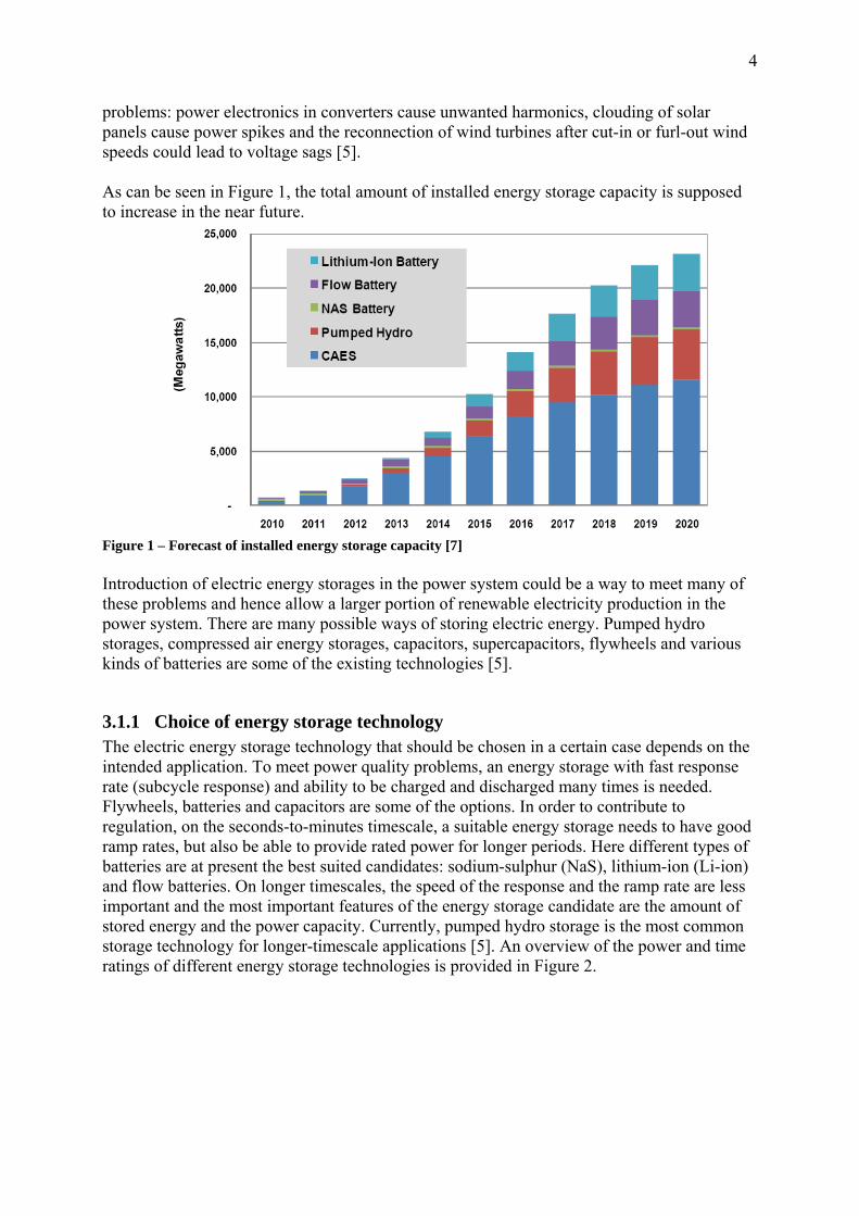
problems: power electronics in converters cause unwanted harmonics, clouding of solar panels cause power spikes and the reconnection of wind turbines after cut-in or furl-out wind speeds could lead to voltage sags [5]. As can be seen in Figure 1, the total amount of installed energy storage capacity is supposed to increase in the near future.

Figure 1 – Forecast of installed energy storage capacity [7] Introduction of electric energy storages in the power system could be a way to meet many of these problems and hence allow a larger portion of renewable electricity production in the power system. There are many possible ways of storing electric energy. Pumped hydro storages, compressed air energy storages, capacitors, supercapacitors, flywheels and various kinds of batteries are some of the existing technologies [5].

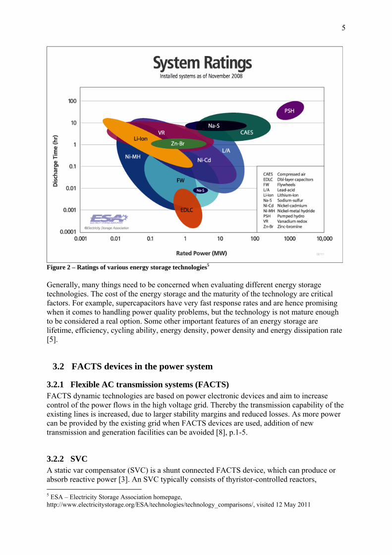
3.1.1 Choice of energy storage technology The electric energy storage technology that should be chosen in a certain case depends on the intended application. To meet power quality problems, an energy storage with fast response rate (subcycle response) and ability to be charged and discharged many times is needed. Flywheels, batteries and capacitors are some of the options. In order to contribute to regulation, on the seconds-to-minutes timescale, a suitable energy storage needs to have good ramp rates, but also be able to provide rated power for longer periods. Here different types of batteries are at present the best suited candidates: sodium-sulphur (NaS), lithium-ion (Li-ion) and flow batteries. On longer timescales, the speed of the response and the ramp rate are less important and the most important features of the energy storage candidate are the amount of stored energy and the power capacity. Currently, pumped hydro storage is the most common storage technology for longer-timescale applications [5]. An overview of the power and time ratings of different energy storage technologies is provided in Figure 2.

5

Figure 2 – Ratings of various energy storage technologies5 Generally, many things need to be concerned when evaluating different energy storage technologies. The cost of the energy storage and the maturity of the technology are critical factors. For example, supercapacitors have very fast response rates and are hence promising when it comes to handling power quality problems, but the technology is not mature enough to be considered a real option. Some other important features of an energy storage are lifetime, efficiency, cycling ability, energy density, power density and energy dissipation rate [5].

3.2 FACTS devices in the power system

3.2.1 Flexible AC transmission systems (FACTS) FACTS dynamic technologies are based on power electronic devices and aim to increase control of the power flows in the high voltage grid. Thereby the transmission capability of the existing lines is increased, due to larger stability margins and reduced losses. As more power can be provided by the existing grid when FACTS devices are used, addition of new transmission and generation facilities can be avoided [8], p.1-5.

3.2.2 SVC A static var compensator (SVC) is a shunt connected FACTS device, which can produce or absorb reactive power [3]. An SVC typically consists of thyristor-controlled reactors, 5 ESA – Electricity Storage Association homepage, http://www.electricitystorage.org/ESA/technologies/technology_comparisons/, visited 12 May 2011

6

thyristor-switched capacitors and filters. The capacitor banks are either connected or disconnected, whereas the thyristor-controlled reactors are variable. Together, a thyristor-controlled reactor and a thyristor-switched capacitor can provide or absorb the exact amount of reactive power needed in the grid at a certain instant [9], p. 471-475. The reactive power is proportional to the voltage squared. Since the reactive power consumed by the transmission lines is proportional to the square of the current and the current varies with the load, the need for reactive power compensation at a certain point in the power system might vary significantly during different load conditions. The reactive power compensation of an SVC is much faster than that of mechanically-switched shunt reactors and shunt capacitors and dynamically controllable. Hence, an SVC can provide rapid control of voltage. This feature is important to maintain voltage stability, especially after disturbances [10]. SVCs are also for example used to mitigate voltage flicker and to increase the stability of the interconnection of two AC systems, by dynamic voltage regulation [9], p. 471-475. A disadvantage of the SVC is that the reactive power delivery capability is reduced at low voltages, when reactive power support to the grid is most needed [10].

3.2.3 STATCOM The static synchronous compensator (STATCOM) consists of a voltage source converter (VSC) and a capacitor bank on the DC side. The current of a VSC can be rapidly controlled, both of magnitude and phase in relation to the AC voltage. This means reactive power can be provided to or absorbed from the connection point with the grid. The capacitor provides a DC voltage and a short-term energy storage for the VSC. The VSC, in turn, maintains a constant voltage over the capacitor and accounts for its own losses by absorbing active power from the grid. The STATCOM performs the same kind of reactive power control as an SVC, but the response of a STATCOM is much faster than that of an SVC. Furthermore, the space requirements are smaller for a STATCOM [9], p. 471-475. In Figure 3 a simplified layout of a STATCOM is shown.

Figure 3 – Basic layout of a STATCOM connected to the grid through a transformer. QSTATCOM is the reactive power delivered to the grid [11].

7

The reactive power delivery capability of a STATCOM is not influenced by low voltages in the same way as the capability of an SVC, which means that the voltage regulation of a STATCOM is more robust than that of an SVC [8], p. 34.

3.3 A changing power system One good example of how the power system is currently changing is the development in Denmark. Historically, the main electricity generation was centralized to large generation units. The power flow was directed from the high voltage transmission grid towards lower voltage distribution grids. With the integration of distributed, often renewable, intermittent electricity sources the power flows are getting bidirectional and unpredictable. The distributed generation units are not treated as dynamic components that could contribute to power balancing and in the case of e.g. wind power the units operate according to weather conditions. The power balancing of the grid is performed by the few large generation units, or transmission lines to other countries or regions [12]. When the wind power production is high and the consumption is low at the same time in a region, there is a surplus of power in the area, which needs to be transmitted to other regions. At the same time, most wind turbines consume reactive power, since they are equipped with asynchronous generators. If the need for reactive power is not compensated locally, it has to be transmitted from the few large generation units, which will lead to greater losses in the transmission lines. The combination of active power production and reactive power consumption at larger wind farms means that the risk that the grid cannot supply the load with power will increase under windy conditions. This would require a reinforced transmission capability, unless the power can be balanced locally. Reinforcement of the grid is costly and could be difficult to perform due to public opposition. This means that distributed active power balancing is favourable [12]. The increasing connection of distributed generation units to the grid also means that centralized control of the power system will be increasingly difficult. Local control will be needed to handle potential problems like loop flows, instabilities, oscillations and over- and undervoltages. FACTS devices could deal with these issues and at the same time reduce the need for new transmission lines or generation units, since the power transfer capability of the existing lines is increased [13].

3.3.1 STATCOM with integrated battery energy storage system (BESS) As a STATCOM is a fast-responding device, it is well suited to help in improving the power quality and stability of wind farms. The reactive power control of the STATCOM can be complemented with active power control if an energy storage is added, for example a battery energy storage [14]. A STATCOM with battery energy storage could control active and reactive power independently, which means that operation in all four quadrants is possible. (See theory, section 4.2, for a more detailed description of four quadrant control). The operating modes are:

• inductive with active power injection into the grid • inductive with active power absorption from the grid • capacitive with active power injection into the grid • capacitive with active power absorption from the grid

8

Even if the STATCOM with battery energy storage can not infinitely operate in one of the quadrants, due to the limitations of the battery energy storage, the device could significantly improve the flexibility and control of the transmission and distribution system [13]. Simulations [14] show that a STATCOM with an integrated battery energy storage could eliminate power fluctuations in the wind turbine output, caused by turbine blades passing the tower. Stability simulations have also been performed. Wind generators are often asynchronous machines, which require reactive power to operate. During voltage sags and faults, the wind turbine will not be able to transmit all of its power into the network. This will cause the speed of the generator to increase, since there is not enough braking electric torque to compensate the driving mechanical torque. This means the slip of the asynchronous generator will increase, thus causing the generator to absorb more reactive power from the grid and further lower the voltage. If the generator speed increases too much, the generator will not be able to return to its normal operation after the fault is cleared. A STATCOM with battery energy storage will increase the stability of wind farms: By supplying reactive power the voltage at the point of common connection will increase, thus increasing the active power output of the wind farm. The output could be increased further if active power is absorbed by the battery energy storage. More active power output from the wind farm means more electrical braking torque in the generators, and thus the stability limit will be increased [14]. Other possible applications are for example voltage control, transmission capacity control, frequency regulation and power oscillation damping. For applications where traditional STATCOMs could also be used, e.g. oscillation damping, the STATCOM with integrated BESS is more flexible, thanks to its ability to also control active power [13].

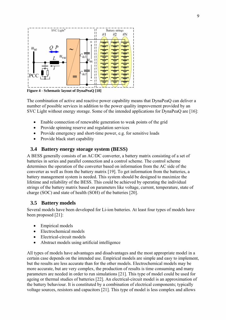
3.3.2 DynaPeaQ DynaPeaQ, the energy storage system developed by ABB, consists of a battery energy storage connected to an SVC Light (the STATCOM developed by ABB) [15]. The energy storage is designed to be used in a power range up to 50 MW and on a timescale from five minutes to one hour. The batteries chosen for the battery energy storage are Li-ion batteries. This type of battery has a relatively long lifetime and good cycling properties for the intended applications [16]. The SVC Light consists of a VSC with IGBT valves. Each phase of the VSC is equipped with a phase reactor and a shunt connected passive filter. Depending on the grid voltage there might also be a need for a transformer between the point of common connection and the filter. A capacitor is connected across the DC side of the VSC [17]. The DC capacitor and the phase reactor are both needed for the VSC to operate properly. If the capacitor voltage becomes too low it will cause overmodulation in the VSC. This limits the ability of the capacitor bank to serve as a short-time energy storage. A realistically dimensioned capacitor could deliver power during fractions of a second. To be able to store energy on a longer timescale, a battery energy storage is connected in parallel with the capacitor. The voltage of the battery energy storage must then be built up to equal the voltage over the DC capacitor. This is done by connecting a large amount of batteries in series, to form a battery string. A number of battery strings could be connected in parallel in order to obtain higher power [17].

9

Figure 4 - Schematic layout of DynaPeaQ [18] The combination of active and reactive power capability means that DynaPeaQ can deliver a number of possible services in addition to the power quality improvement provided by an SVC Light without energy storage. Some of the intended applications for DynaPeaQ are [16]:

• Enable connection of renewable generation to weak points of the grid • Provide spinning reserve and regulation services • Provide emergency and short-time power, e.g. for sensitive loads • Provide black start capability

3.4 Battery energy storage system (BESS) A BESS generally consists of an AC/DC converter, a battery matrix consisting of a set of batteries in series and parallel connection and a control scheme. The control scheme determines the operation of the converter based on information from the AC side of the converter as well as from the battery matrix [19]. To get information from the batteries, a battery management system is needed. This system should be designed to maximize the lifetime and reliability of the BESS. This could be achieved by operating the individual strings of the battery matrix based on parameters like voltage, current, temperature, state of charge (SOC) and state of health (SOH) of the batteries [20].

3.5 Battery models Several models have been developed for Li-ion batteries. At least four types of models have been proposed [21]:

• Empirical models • Electrochemical models • Electrical-circuit models • Abstract models using artificial intelligence

All types of models have advantages and disadvantages and the most appropriate model in a certain case depends on the intended use. Empirical models are simple and easy to implement, but the results are less accurate than for the other models. Electrochemical models may be more accurate, but are very complex, the production of results is time consuming and many parameters are needed in order to run simulations [21]. This type of model could be used for ageing or thermal studies of batteries [22]. An electrical-circuit model is an approximation of the battery behaviour. It is constituted by a combination of electrical components; typically voltage sources, resistors and capacitors [21]. This type of model is less complex and allows

10

shorter calculation times, which is an important feature if the battery model is to be integrated with a larger model for system simulations. However, the parameters of an electrical-circuit model do not correspond to any physical data of the battery [22]. Models using artificial intelligence could be very accurate, but are to a great extent depending on the data used to calibrate them, which means that a model might need to be re-calibrated for each battery, which in turn requires new calibration data [21].

3.6 Different ways of modelling and simulating the power system Many aspects of the power system need to be studied in order to achieve quality, safety and economy in the system. The features studied impact the power system on different timescales and require different modelling and simulation strategies. Steady state conditions in the power system need to be studied, as well as transient phenomena. As the power system is very complex, studying various conditions will always cause a high computational burden. Therefore, several strategies and tools have been developed during the history of the power system. Nowadays, state of the art is to perform simulations using computers [23], p. 1-5.

3.6.1 Steady state The steady state of a power system needs to be known, in order to study whether the generation and transmission capability can sustain the loads in a certain situation. The steady state is also needed as a starting point for simulations of transients. Transmission lines, cables and transformers are modelled using equivalent electric circuits, whereas generators and loads are simply represented by a certain amount of injected or absorbed power at an electrical node in the power system. The voltage and phase angle is determined for all nodes in the system and from this information the steady state power flows through different parts of the transmission system can be calculated [23], p. 12-18.

3.6.2 Short circuits Studying the voltages and currents during a short circuit fault is necessary to dimension the components of the power system correctly. In particular, the breakers must be able to interrupt fault currents. Further, these currents and voltages are inputs to the protection equipment and must therefore be studied to enable the development of protections that adequately detect and locate faults. The modelling of the power system for this type of simulations is similar to the one used for steady state load flow calculations [23], p. 57-66.

3.6.3 Transient conditions Transient stability in a system refers to the retaining of a position of equilibrium after the system has been subject to a sudden disturbance. If, for example, a short circuit causes a major imbalance between the driving and opposing torque of a generator, the machine should not fall out of synchronism. Phenomena related to transient stability usually have time constants between 0.1 and 10 seconds. When studying transient stability phenomena, the machines in the power system need to be modelled in detail, because they determine the dynamic behaviour of the power system under such conditions [23], p. 98-99.

11

3.6.4 The need for real-time digital simulations A real-time system is a system where the time to generate an output is crucial. The correctness of a computation in a real-time system depends not only on the computational result, but also on the time it takes to produce it. Typically, the task of the computer is to monitor or control the operation of some physical equipment. Hence it has to react to physical inputs and produce corresponding outputs sufficiently fast, in order to correctly display or govern the system features [24], p.2-3. It is often very important that real-time systems are reliable, which puts high requirements on the software. Therefore testing of the software is crucial. The testing needs to be performed under all possible operational conditions, in order to debug the software algorithms of errors which could only occur during very rare states of the system. To perform such complex testing actions, a simulator is used. A simulator is a program which behaves in the same way as the physical system into which the real-time software should be embedded. Thus the software can be tested before the real system is completed, but even if the final system already exists simulations can be very useful. Some error states could never be tested on the real system due to safety issues and with a simulator experiments could be repeated more times than would be possible on the real system [24], p. 33-34. Simulations of transient phenomena were traditionally done by using simulators made up of various scaled down power system components physically connected to each other. Another way of simulating the power system behaviour is to use software to make calculations based on a mathematical representation of the system. A main disadvantage of software-based digital simulations is the fact that they are often quite slow. Whereas an analogue simulator made up of scaled down physical components operates in real time, a software-based digital simulator typically require much longer time to produce a solution. For testing of control systems and protection equipment, non-real time operation limits the application of digital simulators [25].

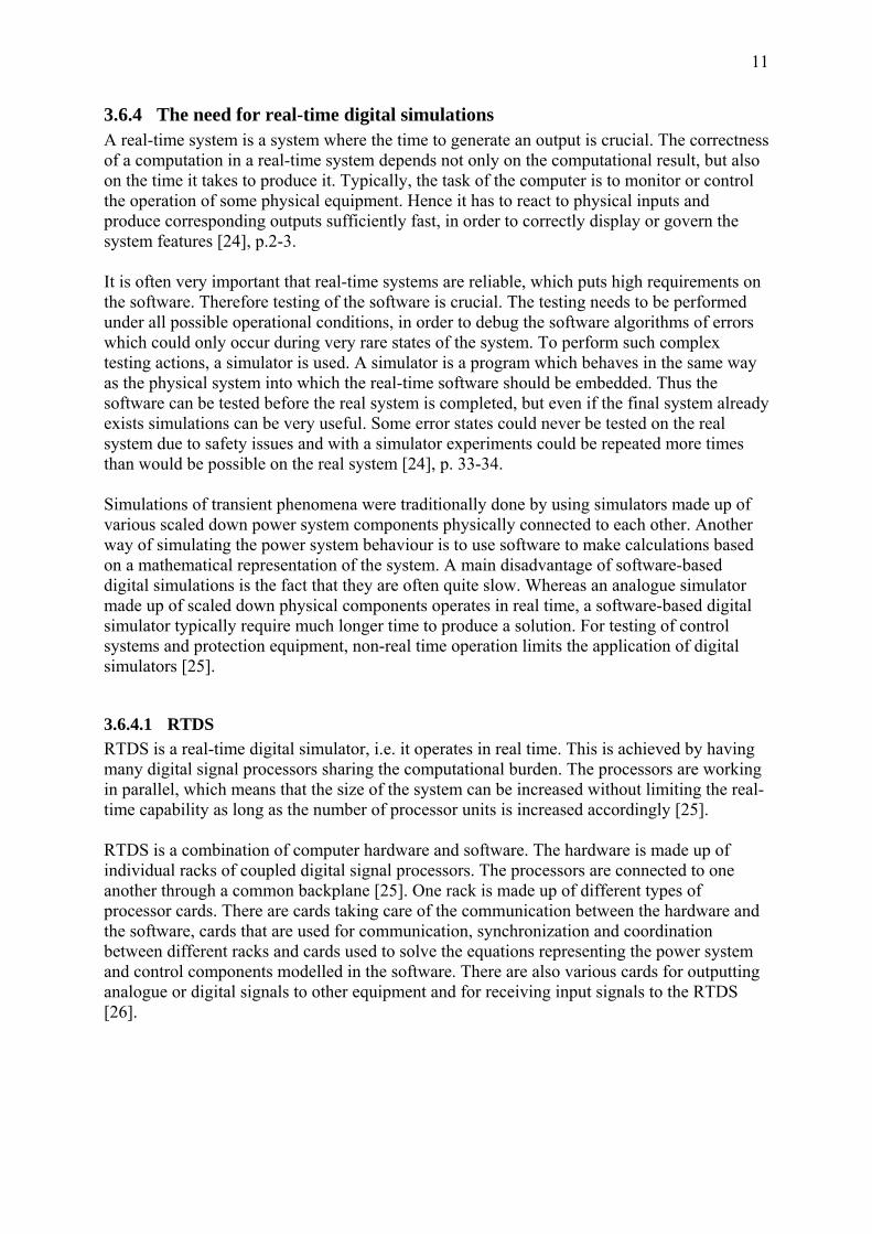
3.6.4.1 RTDS RTDS is a real-time digital simulator, i.e. it operates in real time. This is achieved by having many digital signal processors sharing the computational burden. The processors are working in parallel, which means that the size of the system can be increased without limiting the real-time capability as long as the number of processor units is increased accordingly [25]. RTDS is a combination of computer hardware and software. The hardware is made up of individual racks of coupled digital signal processors. The processors are connected to one another through a common backplane [25]. One rack is made up of different types of processor cards. There are cards taking care of the communication between the hardware and the software, cards that are used for communication, synchronization and coordination between different racks and cards used to solve the equations representing the power system and control components modelled in the software. There are also various cards for outputting analogue or digital signals to other equipment and for receiving input signals to the RTDS [26].

12

Figure 5 – RTDS hardware6 The RTDS software is organized in a three-level hierarchy: a graphical user interface, midlevel compiler and communication and the low-level operating system. The user works only with the highest level, the graphical user interface called RSCAD. In RSCAD/Draft a circuit can be built, using predefined electrical and control components. A simulation performed on the RTDS hardware can be controlled from RSCAD/RunTime [27].

4 Theory

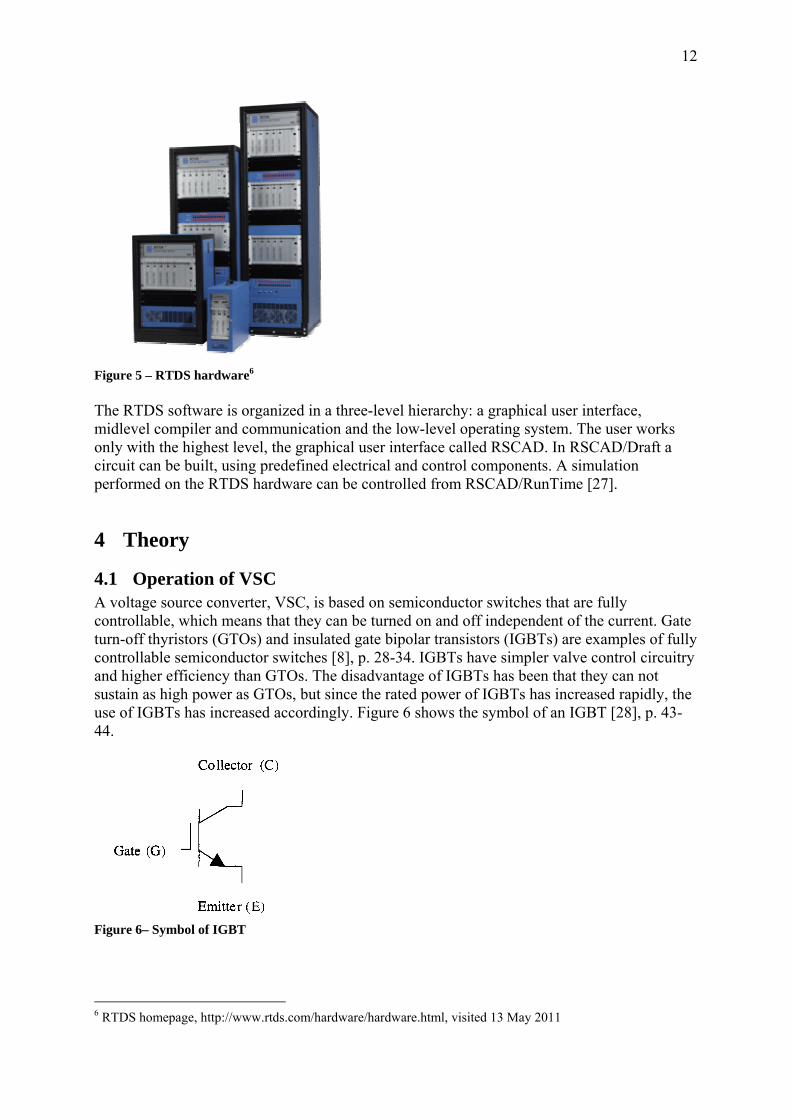
4.1 Operation of VSC A voltage source converter, VSC, is based on semiconductor switches that are fully controllable, which means that they can be turned on and off independent of the current. Gate turn-off thyristors (GTOs) and insulated gate bipolar transistors (IGBTs) are examples of fully controllable semiconductor switches [8], p. 28-34. IGBTs have simpler valve control circuitry and higher efficiency than GTOs. The disadvantage of IGBTs has been that they can not sustain as high power as GTOs, but since the rated power of IGBTs has increased rapidly, the use of IGBTs has increased accordingly. Figure 6 shows the symbol of an IGBT [28], p. 43-44.

Figure 6– Symbol of IGBT

6 RTDS homepage, http://www.rtds.com/hardware/hardware.html, visited 13 May 2011

13

The conventional VSC topology is the three-phase, two-level converter (see Figure 7), with two series connected IGBTs per phase. A diode is connected anti-parallel to each IGBT switch, to take care of voltage reversals and provide a current path in the reverse direction. Capacitors are placed on the DC side, to provide a stiff DC voltage. There are also several other VSC topologies [8], p. 28-34.

Figure 7 - Topology of a three-phase, two-level VSC [8] The control of the VSC governs the switching of the VSC valves in order to modulate an AC waveform as close to a sine wave as possible. At the same time, the aim is to minimize the switching losses and to obtain high power controllability. Thus, the choice of modulation technique is a compromise between generating a sinusoidal AC voltage, in order to minimize the harmonic distortion and hence the need for filters, and to reduce the operating frequency of the semiconductor switches, to reduce the switching losses [8], p. 28-34. The simplest modulation technique is the six-pulse modulation. Using this technique, each phase is switched only twice per period. This makes the fundamental frequency voltage amplitude high, but also causes a large content of low-order harmonics. By switching the valves more often, the voltage becomes nearly sinusoidal, and only high-order harmonics remain, but the fundamental frequency voltage amplitude will also be reduced. For a VSC equipped with IGBTs for high power applications, the switching frequency is normally of the order of magnitude of 1 kHz [28], p. 11-19. By using the pulse width modulation technique (PWM), the frequencies of the first harmonics will be of this order of magnitude as well [28], p. 43-44.

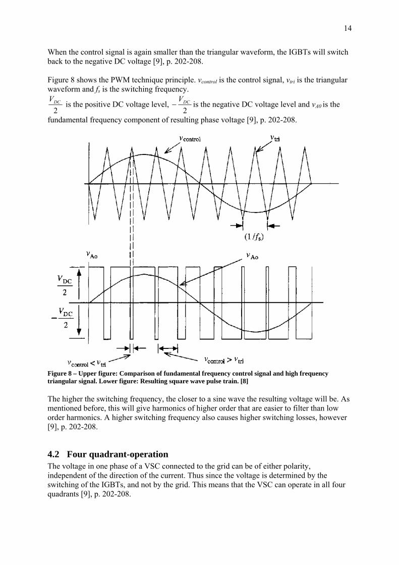
4.1.1 PWM Several PWM techniques have been developed, but the sinusoidal PWM scheme is one of the most used, due to its simplicity and effectiveness. The idea is to build up the sinusoidal voltage waveform for each phase from high-frequency square-wave pulses of variable width, by switching between two DC voltage levels, one positive and one negative [8], p. 28-34. To achieve this, a sinusoidal control signal with the desired frequency is compared with a high-frequency triangular waveform. The frequency of the triangular waveform determines the switching frequency of the inverter. When the control signal gets larger than the triangular waveform, the IGBT valves of the phase leg are operated to switch to the positive DC voltage.

14

When the control signal is again smaller than the triangular waveform, the IGBTs will switch back to the negative DC voltage [9], p. 202-208. Figure 8 shows the PWM technique principle. vcontrol is the control signal, vtri is the triangular waveform and fs is the switching frequency.

2DCV

is the positive DC voltage level, 2DCV

− is the negative DC voltage level and vA0 is the

fundamental frequency component of resulting phase voltage [9], p. 202-208.

Figure 8 – Upper figure: Comparison of fundamental frequency control signal and high frequency triangular signal. Lower figure: Resulting square wave pulse train. [8] The higher the switching frequency, the closer to a sine wave the resulting voltage will be. As mentioned before, this will give harmonics of higher order that are easier to filter than low order harmonics. A higher switching frequency also causes higher switching losses, however [9], p. 202-208.

4.2 Four quadrant-operation The voltage in one phase of a VSC connected to the grid can be of either polarity, independent of the direction of the current. Thus since the voltage is determined by the switching of the IGBTs, and not by the grid. This means that the VSC can operate in all four quadrants [9], p. 202-208.

15

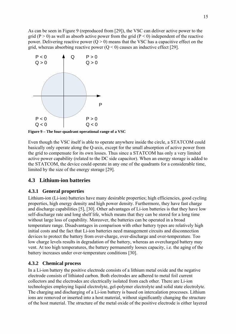
As can be seen in Figure 9 (reproduced from [29]), the VSC can deliver active power to the grid (P > 0) as well as absorb active power from the grid (P < 0) independent of the reactive power. Delivering reactive power (Q > 0) means that the VSC has a capacitive effect on the grid, whereas absorbing reactive power (Q < 0) causes an inductive effect [29].

Q

P

P > 0Q > 0

P > 0Q < 0

P < 0Q < 0

P < 0Q > 0

Figure 9 – The four-quadrant operational range of a VSC Even though the VSC itself is able to operate anywhere inside the circle, a STATCOM could basically only operate along the Q-axis, except for the small absorption of active power from the grid to compensate for its own losses. Thus since a STATCOM has only a very limited active power capability (related to the DC side capacitor). When an energy storage is added to the STATCOM, the device could operate in any one of the quadrants for a considerable time, limited by the size of the energy storage [29].

4.3 Lithium-ion batteries

4.3.1 General properties Lithium-ion (Li-ion) batteries have many desirable properties; high efficiencies, good cycling properties, high energy density and high power density. Furthermore, they have fast charge and discharge capabilities [5], [30]. Other advantages of Li-ion batteries is that they have low self-discharge rate and long shelf life, which means that they can be stored for a long time without large loss of capability. Moreover, the batteries can be operated in a broad temperature range. Disadvantages in comparison with other battery types are relatively high initial costs and the fact that Li-ion batteries need management circuits and disconnection devices to protect the battery from over-charge, over-discharge and over-temperature. Too low charge levels results in degradation of the battery, whereas an overcharged battery may vent. At too high temperatures, the battery permanently looses capacity, i.e. the aging of the battery increases under over-temperature conditions [30].

4.3.2 Chemical process In a Li-ion battery the positive electrode consists of a lithium metal oxide and the negative electrode consists of lithiated carbon. Both electrodes are adhered to metal foil current collectors and the electrodes are electrically isolated from each other. There are Li-ion technologies employing liquid electrolyte, gel-polymer electrolyte and solid state electrolyte. The charging and discharging of a Li-ion battery is based on intercalation processes. Lithium ions are removed or inserted into a host material, without significantly changing the structure of the host material. The structure of the metal oxide of the positive electrode is either layered

16

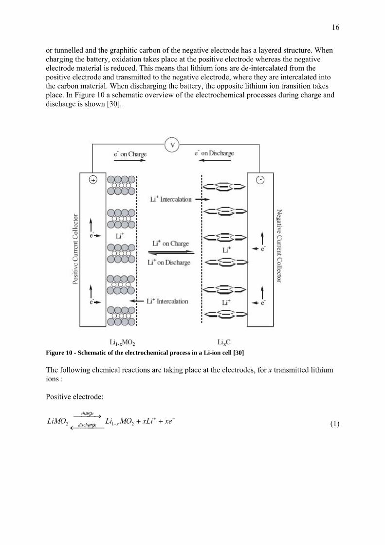
or tunnelled and the graphitic carbon of the negative electrode has a layered structure. When charging the battery, oxidation takes place at the positive electrode whereas the negative electrode material is reduced. This means that lithium ions are de-intercalated from the positive electrode and transmitted to the negative electrode, where they are intercalated into the carbon material. When discharging the battery, the opposite lithium ion transition takes place. In Figure 10 a schematic overview of the electrochemical processes during charge and discharge is shown [30].

Figure 10 - Schematic of the electrochemical process in a Li-ion cell [30] The following chemical reactions are taking place at the electrodes, for x transmitted lithium ions : Positive electrode:

−+− ++

⎯⎯⎯ ⎯←⎯⎯ →⎯

xexLiMOLiLiMO xedisch

ech

212 arg

arg

(1)

17

Negative electrode:

CLixexLiC xedisch

ech

⎯⎯⎯ ⎯←⎯⎯ →⎯

++ −+arg

arg

(2)

LiMO2 represents the lithium metal oxide material of the positive electrode and C represents the carbon material of the negative electrode [30].

4.3.3 The batteries used for DynaPeaQ The battery cells used for DynaPeaQ are liquid electrolyte cells, with lithiated nickel oxide as a positive electrode. There are three main types of cells provided by Saft: high energy cells, which are optimized to provide energy on longer timescales, high power cells, which provide high power on shorter time scales and medium range cells, which are a compromise between energy content and power capability [31]. The batteries are ageing in two ways: by calendar ageing and due to operational use. Calendar ageing means that the batteries will lose a certain amount of their capability even if they are not used. This ageing phenomenon is mainly caused by interactions between electrolyte and active materials. Ageing due to operational use depends on how the battery is cycled. This type of aging decreases the material reversibility in the battery cell. Supposing that end of life of a battery cell occurs when the battery capability has decreased to 80 % of the original capability, results from Saft show that the batteries used for DynaPeaQ have good lifetime properties [31]. The batteries survive more than three thousand deep cycles (of 80 % depth of discharge) [16] and several thousand shallow cycles. The minimum lifetime of the cells is 6-20 years, depending on how the battery is operated [31].

4.3.4 Polarization The voltage of a battery cell may be regarded as the electrical potential difference between the electrodes of the cell. If no current flows through the battery cell, the measurable potential difference is the equilibrium cell voltage [32]. This equilibrium voltage is also called the open circuit voltage (OCV) [33]. If a voltage applied to the cell terminals does not exactly equal the equilibrium voltage, a current will flow and the terminal voltage of the cell will shift from its equilibrium value. This changing of cell voltage when a current flows through the cell is called ‘polarization’. The magnitude of the voltage shift caused by polarization is called ‘overvoltage’. The sign of the overvoltage is usually positive for a cell being charged and negative for a cell being discharged, i.e. the terminal voltage of a cell is higher on charge than on discharge [32]. Several effects contribute to the polarization. The three main polarization components are ohmic polarization, concentration polarization and activation polarization. Any of these polarization components may be dominant, depending on the circumstances. In some cases, the charging of the double layer and dissipation phenomena could also give rise to important polarizations. All these polarization components give rise to overvoltages. The total overvoltage is the sum of these contributions [32].

18

4.3.4.1 Ohmic overvoltage The ohmic overvoltage is caused by the resistance of the ionic conductor, and follows Ohm’s law [32]:

IRV ohmicohmic ⋅=

(3)

The resistance of the solid phase material is small compared to the resistance of the electrolyte. There is also a contact resistance. The contact resistance is constant for a given current, whereas the resistance of the ionic conductor increases slightly with time [34]. The ohmic resistance should usually be independent of the SOC level [35] and the ageing of the battery cell [36].

4.3.4.2 Concentration overvoltage When the battery is charged or discharged, chemical reactions take place at the electrodes (according to equations (1) and (2)). This means that reactants will be consumed and products will be created. Thus, the concentrations of these species at the electrode surface get disturbed. This gives rise to the concentration overvoltage or, differently stated, the concentration overvoltage is the ‘extra’ voltage needed to keep the reaction rate despite the concentration disturbance, and thus provide the requested current [32]. The concentration overvoltage can be expressed as

⎭⎬⎫

⎩⎨⎧

<<

=)()0()0()(ln

tctctctc

nFRTV s

RsP

sR

sP

conc

(4)

where R is the universal gas constant, T is the absolute temperature, n is the number of moles of electrons transferred in the cell reaction, F is the Faraday constant, )0( <tcs

P and )0( <tcsR

are the concentrations of products and reactants, respectively, at the electrode surface, before the experiment starts, while )(tcs

P and )(tcsR are the corresponding concentrations at the time

t. Even though the current is not directly involved in the equation, it strongly influences the magnitude of the concentration overvoltage. The current is directly proportional to the destruction rate of the reactants and the creation rate of the products, but how these rates exactly influences the surface concentrations is decided by cell geometry and transport mechanisms. The concentration polarization is mainly located in the thin transport layer surrounding the electrodes [32].

4.3.4.3 Activation overvoltage The activation overvoltage is related to the kinetic of the reaction taking place at the electrode surface [22]. Many spontaneous reactions are slow, because they require a certain activation energy. This energy is the minimum energy that must be present if a collision between two atoms or molecules is to result in a chemical reaction. Since an increased temperature results in higher average thermal energy among the atoms and molecules, it will generally lead to higher reaction rates [37]. In the case of a lithium-ion battery, the electron-transfer reaction is rather slow. The activation overvoltage provides the extra power needed to force the reaction to proceed at the speed required by the current. A change in temperature has a major effect on

19

the activation overvoltage [32]. The activation overvoltage, Vact(t), can be related to the current as follows:

[ ] [ ] ⎥⎦

⎤⎢⎣

⎡−∗∗=

−− RT

tnFVRT

tnFVsP

sR

actact

eetctcnFAktI)()1()(

1 )()()(ββ

ββ

(5)

I(t) is the current, A is the electrode area, k is the rate constant of the electron-transfer reaction, β is the transfer coefficient of the same reaction and the other parameters have the same meanings as above. The equation cannot be inverted to give an explicit expression for Vact except for some discrete values of β, but Vact can easily be found through iteration [32]. The activation overvoltage is more or less constant with time, as long as the current or the temperature do not change. The activation polarization is more significant in the positive electrode than in the negative [34].

4.3.4.4 Diffusion overvoltage A lithium-ion battery has porous electrodes, into which the lithium ions diffuse. This causes energy dissipation and concentration gradients. During a discharge a negative overvoltage, i.e. a voltage drop compared to the OCV occurs. The diffusion overvoltage increases very slowly with time [22]. However, the increase is large. From being close to zero at the start of the discharge, the diffusion overvoltage evolves to become one of the most significant contributions to the total cell overvoltage, after some tens of seconds [34]. When the discharge is stopped the lithium-ion concentration in the electrodes slowly get uniform again, due to the same diffusion phenomena. This is called relaxation [22]. A corresponding diffusion overvoltage also occurs in the electrolyte. The diffusion polarization is more important in the negative electrode than in the positive [34]. If, for example, a charging of the battery cell is initiated a short time after a discharge has been finished, the diffusion polarization actually decreases the total cell polarization during a short time period. This phenomenon is caused by the fact that the concentration gradients that were built up during the discharge are still present, since the cell has not had time to relax completely, and the concentration profiles facilitate the charging process [34].

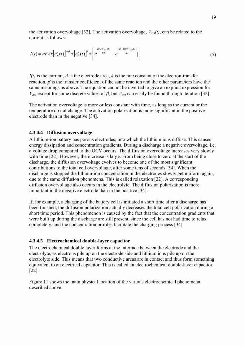
4.3.4.5 Electrochemical double-layer capacitor The electrochemical double layer forms at the interface between the electrode and the electrolyte, as electrons pile up on the electrode side and lithium ions pile up on the electrolyte side. This means that two conductive areas are in contact and thus form something equivalent to an electrical capacitor. This is called an electrochemical double-layer capacitor [22]. Figure 11 shows the main physical location of the various electrochemical phenomena described above.

20

Figure 11 – Overview of the location of electrochemical phenomena. The figure is based on [32] and [22].

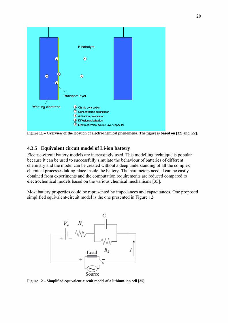
4.3.5 Equivalent circuit model of Li-ion battery Electric-circuit battery models are increasingly used. This modelling technique is popular because it can be used to successfully simulate the behaviour of batteries of different chemistry and the model can be created without a deep understanding of all the complex chemical processes taking place inside the battery. The parameters needed can be easily obtained from experiments and the computation requirements are reduced compared to electrochemical models based on the various chemical mechanisms [35]. Most battery properties could be represented by impedances and capacitances. One proposed simplified equivalent-circuit model is the one presented in Figure 12:

Figure 12 – Simplified equivalent-circuit model of a lithium-ion cell [35]

21

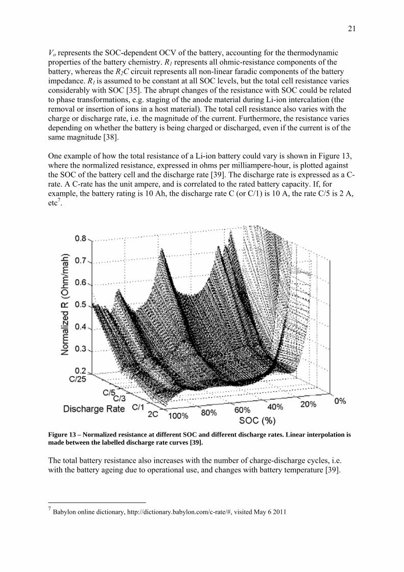
Vo represents the SOC-dependent OCV of the battery, accounting for the thermodynamic properties of the battery chemistry. R1 represents all ohmic-resistance components of the battery, whereas the R2C circuit represents all non-linear faradic components of the battery impedance. R1 is assumed to be constant at all SOC levels, but the total cell resistance varies considerably with SOC [35]. The abrupt changes of the resistance with SOC could be related to phase transformations, e.g. staging of the anode material during Li-ion intercalation (the removal or insertion of ions in a host material). The total cell resistance also varies with the charge or discharge rate, i.e. the magnitude of the current. Furthermore, the resistance varies depending on whether the battery is being charged or discharged, even if the current is of the same magnitude [38]. One example of how the total resistance of a Li-ion battery could vary is shown in Figure 13, where the normalized resistance, expressed in ohms per milliampere-hour, is plotted against the SOC of the battery cell and the discharge rate [39]. The discharge rate is expressed as a C-rate. A C-rate has the unit ampere, and is correlated to the rated battery capacity. If, for example, the battery rating is 10 Ah, the discharge rate C (or C/1) is 10 A, the rate C/5 is 2 A, etc7.

Figure 13 – Normalized resistance at different SOC and different discharge rates. Linear interpolation is made between the labelled discharge rate curves [39]. The total battery resistance also increases with the number of charge-discharge cycles, i.e. with the battery ageing due to operational use, and changes with battery temperature [39].

7 Babylon online dictionary, http://dictionary.babylon.com/c-rate/#, visited May 6 2011

22

5 Models used The RTDS model was to be partly based on existing models: A Matlab/Simulink model of a battery cell provided by the battery manufacturer and a PSCAD model of an SVC Light with a simplified energy storage, already developed at FACTS.

5.1 The Matlab/Simulink model The battery manufacturer, Saft, has provided a Simulink model, where a battery cell is implemented as a black box, with certain inputs and outputs. Among the user-definable inputs to the black-box Simulink model are:

• initial SOC of the battery cell • ageing of the battery cell • initial battery temperature • external temperature • input current • heat exchange coefficient related to the battery cell surface

Simulations can be run for a time chosen, with a time step of 100 ms. Charges and discharges at different rates can thus be performed under various conditions. Outputs from the black-box model are, among others:

• terminal voltage of the battery cell • temperature of the battery • SOC of the battery • maximum capacity of the battery cell under the given conditions

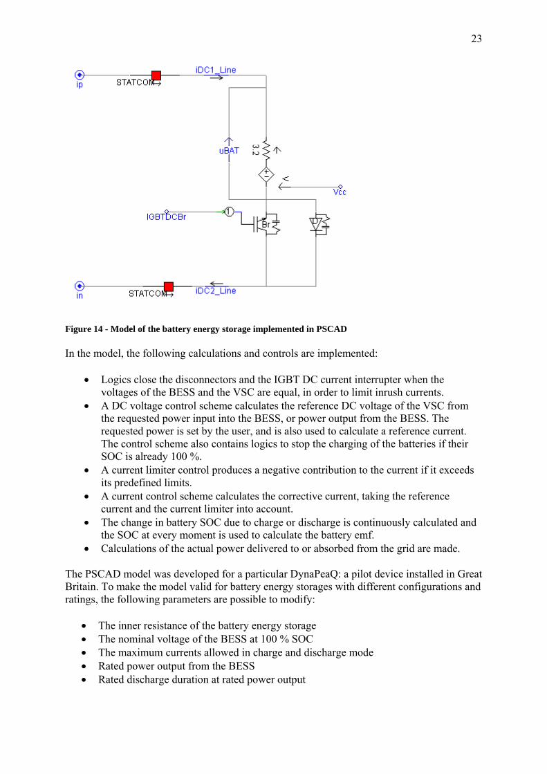
5.2 The PSCAD model A simplified model of the battery energy storage had previously been implemented in the simulation program PSCAD, together with a model of the SVC Light. This model can be used to simulate the connection of the battery energy storage to the SVC Light and operation of the storage in charge, discharge and floating mode. In the PSCAD model, the battery energy storage is simply modelled as a single DC voltage source behind a resistance. One IGBT DC current interrupter and two disconnectors are also present. The purpose of the IGBT DC current interrupter is to limit the current, so that the disconnectors can be operated. The DC voltage of the source varies depending on the state of charge of the batteries, according to a table provided by Saft that relates open circuit voltage to SOC. The power flow into the batteries, when charging, or out of the batteries, when discharging, is determined by the voltage difference between the battery DC voltage source and the voltage over the capacitors on the DC side of the converter. If the capacitor voltage is higher than the battery voltage, the batteries will be charged, whereas a lower capacitor voltage will lead to discharge of the batteries. Figure 14 shows the part of the model representing the battery energy storage.

23

Figure 14 - Model of the battery energy storage implemented in PSCAD In the model, the following calculations and controls are implemented:

• Logics close the disconnectors and the IGBT DC current interrupter when the voltages of the BESS and the VSC are equal, in order to limit inrush currents.

• A DC voltage control scheme calculates the reference DC voltage of the VSC from the requested power input into the BESS, or power output from the BESS. The requested power is set by the user, and is also used to calculate a reference current. The control scheme also contains logics to stop the charging of the batteries if their SOC is already 100 %.

• A current limiter control produces a negative contribution to the current if it exceeds its predefined limits.

• A current control scheme calculates the corrective current, taking the reference current and the current limiter into account.

• The change in battery SOC due to charge or discharge is continuously calculated and the SOC at every moment is used to calculate the battery emf.

• Calculations of the actual power delivered to or absorbed from the grid are made. The PSCAD model was developed for a particular DynaPeaQ: a pilot device installed in Great Britain. To make the model valid for battery energy storages with different configurations and ratings, the following parameters are possible to modify:

• The inner resistance of the battery energy storage • The nominal voltage of the BESS at 100 % SOC • The maximum currents allowed in charge and discharge mode • Rated power output from the BESS • Rated discharge duration at rated power output

24

To simulate different situations, the user can specify the following parameters before each run:

• Required power output from the BESS or power input to the BESS • Initial SOC of the batteries • Time to close the disconnectors • Position of the switch to switch on the IGBT DC current interrupter if the BESS is to

be discharged. (The switch outputs the signal IGBTDCBr, shown in Figure 14).

6 Modelling The aim was to develop a simple, aggregated model for testing of charge and discharge regimes in RTDS. The BESS should be constantly connected and in operation. The connection or disconnection of the energy storage was not to be tested on this model. Neither was the communication of the DynaPeaQ master control system with the battery management system. The power into or out of the energy storage is to be controlled by the converter control system at a later stage, though. However, a simple voltage control was needed inside the RTDS model, to be able to test it. Even though the model should be a very simple one, the aim was to mimic the behaviour of the batteries as closely as possible, in order to generate a correct terminal voltage and SOC level of the battery energy storage. These features are critical, since they determine how much power the energy storage could deliver under different conditions. Thus they need to be considered when dimensioning the energy storage part of DynaPeaQ for different applications and requirements. The RTDS model was intended to include many features from the Simulink model as well as from the PSCAD model. The PSCAD model was used as a starting point when developing the RTDS model. The Simulink model was used to find an approximate model of how the battery properties change with different parameters; temperature, SOC, current and ageing.

6.1 Layout of the RTDS model The layout of the RTDS model was based on the existing PSCAD model. Some of the control schemes could be directly transferred to RSCAD and some were used with small modifications. The approach was to represent the BESS with a variable DC voltage source behind a resistance, as in the PSCAD model. The resistance of the batteries in the RTDS model was to be variable. The disconnectors and the IGBT DC current interrupter were excluded from the model. Thus since the model was only intended to be used for simulations of an already connected energy storage, which means that the disconnectors and the IGBT DC current interrupter would not play a significant role. From the point of view of the battery energy storage, the most important feature of the grid interface, i.e. the SVC Light, is the DC voltage over the capacitor. The difference between this voltage and the battery voltage decides the power flow into or out of the batteries. Since the purpose of the model was to study the charge and discharge of the batteries, it was decided that it would be sufficient to represent the VSC of the SVC Light as a variable voltage source, just like the voltage source representing the emf of the BESS. The voltage level of the VSC

25

variable voltage source was decided by simply taking the reference DC voltage as input to the component. Most of the control functions in the existing PSCAD model would still be needed in the RTDS model, except the ones dealing with connection or disconnection of the BESS. The following functions were considered to be necessary:

• The DC voltage control scheme to calculate the reference DC voltage of the VSC and the reference current from the power set by the user, with logics to stop the charging of the batteries if the SOC is too high.

• The current limiter control. • The control scheme to calculate the change in battery SOC due to charge or discharge

and the battery emf. • The calculation of the actual power delivered to or absorbed from the grid.

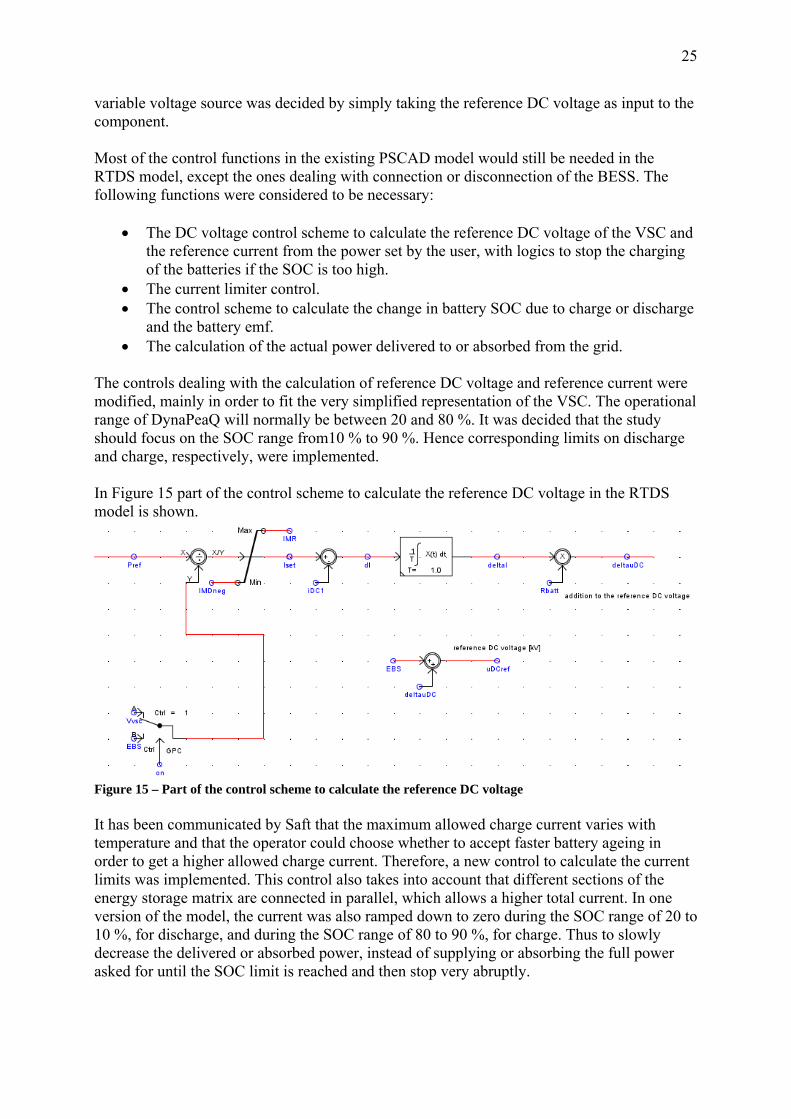
The controls dealing with the calculation of reference DC voltage and reference current were modified, mainly in order to fit the very simplified representation of the VSC. The operational range of DynaPeaQ will normally be between 20 and 80 %. It was decided that the study should focus on the SOC range from10 % to 90 %. Hence corresponding limits on discharge and charge, respectively, were implemented. In Figure 15 part of the control scheme to calculate the reference DC voltage in the RTDS model is shown.

Figure 15 – Part of the control scheme to calculate the reference DC voltage It has been communicated by Saft that the maximum allowed charge current varies with temperature and that the operator could choose whether to accept faster battery ageing in order to get a higher allowed charge current. Therefore, a new control to calculate the current limits was implemented. This control also takes into account that different sections of the energy storage matrix are connected in parallel, which allows a higher total current. In one version of the model, the current was also ramped down to zero during the SOC range of 20 to 10 %, for discharge, and during the SOC range of 80 to 90 %, for charge. Thus to slowly decrease the delivered or absorbed power, instead of supplying or absorbing the full power asked for until the SOC limit is reached and then stop very abruptly.

26

Similarly, the current is ramped down if the battery terminal voltage approaches its limits; 4V and 3V, respectively. If the voltage exceeds 3.9 V in charging regime or if it undercuts 3.1 in discharging regime, the current is linearly ramped down, to reach zero when the voltage limit is reached. These continuously calculated current limits were directly integrated into the DC voltage and current control scheme. The control scheme to calculate battery emf and changes in SOC, as well as the control to calculate the actual power were kept more or less unchanged compared to the PSCAD model, except that the SOC calculation was adjusted to work properly for energy storages of different ratings and layout. Further, some new controls and features not present in the PSCAD model were added to the RTDS model:

• Some sliders to set dimensioning parameters of the BESS, such as the number of rooms per string and the number of strings in parallel. The settings are used as inputs to controls calculating parameters necessary for other control schemes, like e.g. the rated voltage of the battery energy storage.

• Controls that calculate voltage and current at battery cell level, for evaluation purposes.

• Control schemes to obtain the resistive behaviour of the batteries, depending on a number of parameters.

• A simple control calculating the losses of the batteries. • A control calculating the temperature of the batteries, based on the external

temperature, the initially set battery temperature and the current. • Some selector controls and a couple of switches to operate them, in order to avoid

computational problems at the initiation of a simulation.

6.2 Investigation of battery resistance The Simulink model was used to investigate how the battery resistance varies with different parameters. The initial approach was to keep the resistance model as simple as possible and reduce the number of dependencies on other parameters. However, during the investigations it turned out that many factors influenced the battery resistance so significantly that they had to be included in the model. A first attempt to approximate the resistance was to derive a table from the model, showing how the resistance varies with the SOC of the batteries. This was done by recording the battery voltage for different SOC levels for a certain current into or out from the battery cell. When looking at the cell as a Thevenin equivalent, this information could be combined with the table of OCV versus SOC provided by Saft to approximate the resistance for different SOC levels.

27

Figure 16 – Thevenin equivalent representation of battery cell Figure 16 shows the Thevenin equivalent of the battery cell. E is the emf of the battery, by definition equal to the open circuit voltage. R is the inner resistance of the battery and Vterminal is the terminal voltage of the cell. The model that was investigated represented the high power cell type. During communication with Saft [40] it was clarified that the total resistance of a battery is constituted by an ohmic resistance and an additional chemical impedance. The ohmic resistance causes heat losses, and could be seen as a normal resistance even from an electrical point of view. The chemical impedance, on the other hand, does not cause any losses. It just temporarily reduces the capacity of the battery at discharge by reducing the terminal voltage, thus forcing the current to increase in order to provide the same amount of power at the terminals. If a current limit is reached, the battery will not be able to deliver the requested power, even if there is still energy left in the battery [40]. Cf. the presentation of different polarization phenomena in the sections 4.3.4.1, 4.3.4.2, 4.3.4.3 and 4.3.4.4. In order to understand the resistance variations and get a more realistic model of the BESS, where e.g. losses could be accounted for, it was decided that the resistance should be divided into two parts: Rohmic, which gives rise to heat losses and Rchemical, which causes a voltage drop, but does not contribute to the resistive losses. The approach was then to see a battery cell (or the BESS as a whole, when aggregating many cells) as a Thevenin equivalent with two separate resistances, as can be seen in Figure 17.

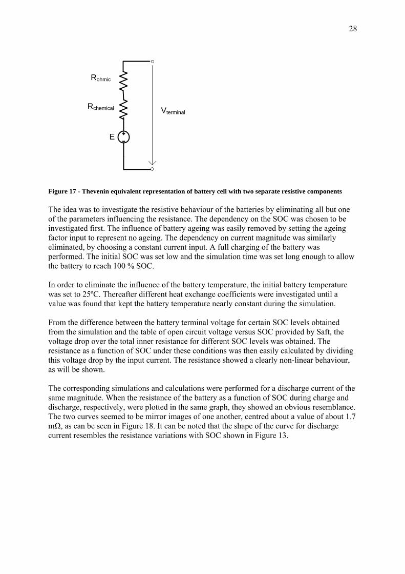
28

E

Rchemical

Rohmic

Vterminal

Figure 17 - Thevenin equivalent representation of battery cell with two separate resistive components The idea was to investigate the resistive behaviour of the batteries by eliminating all but one of the parameters influencing the resistance. The dependency on the SOC was chosen to be investigated first. The influence of battery ageing was easily removed by setting the ageing factor input to represent no ageing. The dependency on current magnitude was similarly eliminated, by choosing a constant current input. A full charging of the battery was performed. The initial SOC was set low and the simulation time was set long enough to allow the battery to reach 100 % SOC. In order to eliminate the influence of the battery temperature, the initial battery temperature was set to 25ºC. Thereafter different heat exchange coefficients were investigated until a value was found that kept the battery temperature nearly constant during the simulation. From the difference between the battery terminal voltage for certain SOC levels obtained from the simulation and the table of open circuit voltage versus SOC provided by Saft, the voltage drop over the total inner resistance for different SOC levels was obtained. The resistance as a function of SOC under these conditions was then easily calculated by dividing this voltage drop by the input current. The resistance showed a clearly non-linear behaviour, as will be shown. The corresponding simulations and calculations were performed for a discharge current of the same magnitude. When the resistance of the battery as a function of SOC during charge and discharge, respectively, were plotted in the same graph, they showed an obvious resemblance. The two curves seemed to be mirror images of one another, centred about a value of about 1.7 mΩ, as can be seen in Figure 18. It can be noted that the shape of the curve for discharge current resembles the resistance variations with SOC shown in Figure 13.

29

0

0.5

1

1.5

2

2.5

100 90 80 70 60 50 40 30 20 10

SOC

Rto

t [m

ohm

]

Rtot @ 50A, dischargeRtot @ 50A, charge

Figure 18 – Total resistance of new batteries as a function of SOC calculated from run of the Simulink model at a constant temperature of 25ºC during charge and discharge

With the discussion with Saft in mind and because of the appearance of the graph, it was assumed that Rohmic might be a relatively constant resistance with a value somewhere in between the mirrored curves, whereas the non-ohmic resistance might be responsible for the deviations from that value.

6.2.1 Ohmic resistance To test this hypothesis, Rohmic was calculated using another method: Since resistive losses dissipate as heat, Rohmic should be obtainable from the heat generated by a battery cell during the simulation. If the internal temperature of the battery does not change during the simulation, the heat power generated should correspond to the heat exchange coefficient related to the battery cell surface. The heat exchange coefficient has the unit W/(m2K). The equation to obtain the heat power is then

TAhP cellheat Δ= ** (6) where h is the heat exchange coefficient, Acell is the surface area of the battery cell and ΔT is the temperature difference between the battery and the ambient. Since the heat exchange coefficient to keep the internal battery temperature almost constant was already determined and the external temperature is decided by the user, h and ΔT were constants already at hand for the simulated conditions. The surface area of a battery cell was calculated from information about height and diameter of the battery cell types used for DynaPeaQ, obtained from product data sheets available at the Saft homepage8. Thus, the heat power could be obtained. On the other hand, the heat power could be expressed as

8 Saft homepage, http://www.saftbatteries.com/Technologies_Lithium_Liion_301/Language/en-US/Default.aspx, visited 12 March 2011

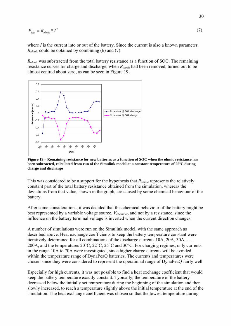
30

2* IRP ohmicheat = (7)

where I is the current into or out of the battery. Since the current is also a known parameter, Rohmic could be obtained by combining (6) and (7). Rohmic was substracted from the total battery resistance as a function of SOC. The remaining resistance curves for charge and discharge, when Rohmic had been removed, turned out to be almost centred about zero, as can be seen in Figure 19.

-0.8

-0.6

-0.4

-0.2

0

0.2

0.4

0.6

0.8

100 90 80 70 60 50 40 30 20 10

SOC

Rche

mic

al [m

ohm

]

Rchemical @ 50A dischargeRchemical @ 50A charge

Figure 19 – Remaining resistance for new batteries as a function of SOC when the ohmic resistance has been subtracted, calculated from run of the Simulink model at a constant temperature of 25ºC during charge and discharge

This was considered to be a support for the hypothesis that Rohmic represents the relatively constant part of the total battery resistance obtained from the simulation, whereas the deviations from that value, shown in the graph, are caused by some chemical behaviour of the battery.

After some considerations, it was decided that this chemical behaviour of the battery might be best represented by a variable voltage source, Vchemical, and not by a resistance, since the influence on the battery terminal voltage is inverted when the current direction changes. A number of simulations were run on the Simulink model, with the same approach as described above. Heat exchange coefficients to keep the battery temperature constant were iteratively determined for all combinations of the discharge currents 10A, 20A, 30A, …, 200A, and the temperatures 20°C, 22°C, 25°C and 30°C. For charging regimes, only currents in the range 10A to 70A were investigated, since higher charge currents will be avoided within the temperature range of DynaPeaQ batteries. The currents and temperatures were chosen since they were considered to represent the operational range of DynaPeaQ fairly well. Especially for high currents, it was not possible to find a heat exchange coefficient that would keep the battery temperature exactly constant. Typically, the temperature of the battery decreased below the initially set temperature during the beginning of the simulation and then slowly increased, to reach a temperature slightly above the initial temperature at the end of the simulation. The heat exchange coefficient was chosen so that the lowest temperature during

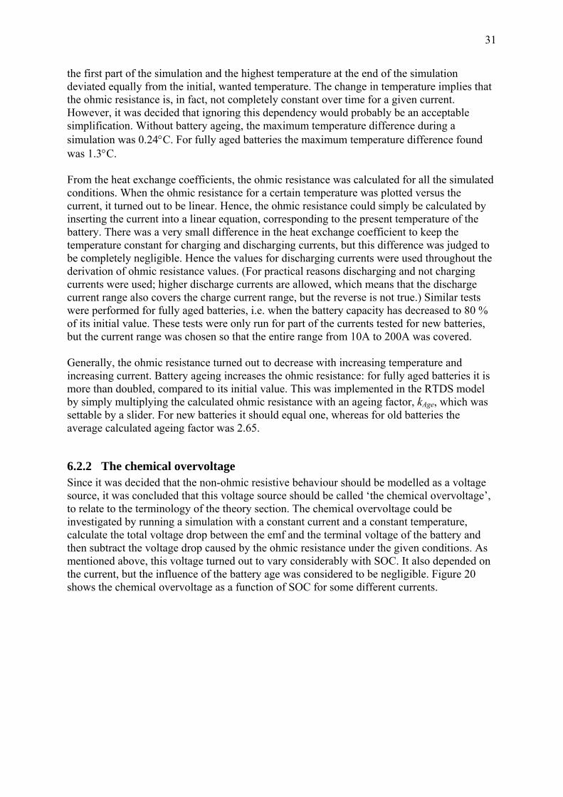
31

the first part of the simulation and the highest temperature at the end of the simulation deviated equally from the initial, wanted temperature. The change in temperature implies that the ohmic resistance is, in fact, not completely constant over time for a given current. However, it was decided that ignoring this dependency would probably be an acceptable simplification. Without battery ageing, the maximum temperature difference during a simulation was 0.24°C. For fully aged batteries the maximum temperature difference found was 1.3°C. From the heat exchange coefficients, the ohmic resistance was calculated for all the simulated conditions. When the ohmic resistance for a certain temperature was plotted versus the current, it turned out to be linear. Hence, the ohmic resistance could simply be calculated by inserting the current into a linear equation, corresponding to the present temperature of the battery. There was a very small difference in the heat exchange coefficient to keep the temperature constant for charging and discharging currents, but this difference was judged to be completely negligible. Hence the values for discharging currents were used throughout the derivation of ohmic resistance values. (For practical reasons discharging and not charging currents were used; higher discharge currents are allowed, which means that the discharge current range also covers the charge current range, but the reverse is not true.) Similar tests were performed for fully aged batteries, i.e. when the battery capacity has decreased to 80 % of its initial value. These tests were only run for part of the currents tested for new batteries, but the current range was chosen so that the entire range from 10A to 200A was covered. Generally, the ohmic resistance turned out to decrease with increasing temperature and increasing current. Battery ageing increases the ohmic resistance: for fully aged batteries it is more than doubled, compared to its initial value. This was implemented in the RTDS model by simply multiplying the calculated ohmic resistance with an ageing factor, kAge, which was settable by a slider. For new batteries it should equal one, whereas for old batteries the average calculated ageing factor was 2.65.

6.2.2 The chemical overvoltage Since it was decided that the non-ohmic resistive behaviour should be modelled as a voltage source, it was concluded that this voltage source should be called ‘the chemical overvoltage’, to relate to the terminology of the theory section. The chemical overvoltage could be investigated by running a simulation with a constant current and a constant temperature, calculate the total voltage drop between the emf and the terminal voltage of the battery and then subtract the voltage drop caused by the ohmic resistance under the given conditions. As mentioned above, this voltage turned out to vary considerably with SOC. It also depended on the current, but the influence of the battery age was considered to be negligible. Figure 20 shows the chemical overvoltage as a function of SOC for some different currents.

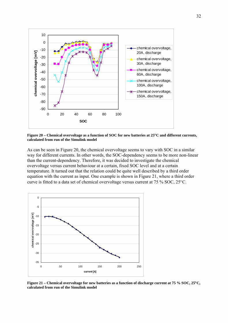
32

-90

-80

-70

-60

-50

-40

-30

-20

-10

0

10

0 20 40 60 80 100

SOC

chem

ical

ove

rvol

tage

[mV]

chemical overvoltage,20A, discharge

chemical overvoltage,30A, discharge

chemical overvoltage,60A, discharge

chemical overvoltage,100A, discharge

chemical overvoltage,150A, discharge

Figure 20 – Chemical overvoltage as a function of SOC for new batteries at 25°C and different currents, calculated from run of the Simulink model As can be seen in Figure 20, the chemical overvoltage seems to vary with SOC in a similar way for different currents. In other words, the SOC-dependency seems to be more non-linear than the current-dependency. Therefore, it was decided to investigate the chemical overvoltage versus current behaviour at a certain, fixed SOC level and at a certain temperature. It turned out that the relation could be quite well described by a third order equation with the current as input. One example is shown in Figure 21, where a third order curve is fitted to a data set of chemical overvoltage versus current at 75 % SOC, 25°C.

-35

-30

-25

-20

-15

-10

-5

0

0 50 100 150 200 250

current [A]

chem

ical

ove

rvol

tage

[mV]

Figure 21 – Chemical overvoltage for new batteries as a function of discharge current at 75 % SOC, 25°C, calculated from run of the Simulink model

33

The corresponding equations were found for SOC levels of 10 %, 15 %, … , 90 %. The equations were derived for the temperatures 20°C, 25°C and 30°C. The equations for 20°C and 25°C approximately coincided for all SOC levels and currents, whereas the equation for 30°C deviated a little from the others for very low currents (10 A) and for high currents at low SOC levels (at most for currents larger than 150 A at 10 % SOC). Despite this, it was considered to be an acceptable approximation to use the set of equations obtained for 25°C for all temperatures in the range. Thus since a lower temperature would lead to a more or less correct value of Vchemical whereas a higher temperature would lead to a somewhat larger value of Vchemical than the one obtained with the Simulink model, which would lead to a lower terminal voltage of the battery. During discharge, this would mean that it would be somewhat more difficult to deliver a certain amount of power to the grid, i.e. a higher current would be needed than if the value of Vchemical obtained from the Simulink model would be used. During charge, a larger current would similarly be needed to feed a certain amount of power into the batteries if the set of equations were used, compared to if the Simulink model were used. In other words, adopting the equations for 25°C even at higher temperature should lead to a conservative approximation of Vchemical. When fitting the third order curves to the data, it was disregarded that the chemical overvoltage should be equal to zero when no current flows through the battery (cf. Figure 21). Thus since the battery terminal voltage should, by definition, be equal to the OCV, i.e. the emf, when no current flows. Disregarding this should lead to a somewhat too low terminal voltage at no current for most SOC levels. In particular, the terminal voltage will be too low at SOC levels where the chemical overvoltage has a large, negative value even for low currents, e.g. at 70 % SOC (cf. Figure 20). At high SOC levels, the magnitude of the chemical overvoltage was considerably larger for charge currents than for discharge currents. However, this was disregarded and the equations obtained for discharge currents were used independent of the current direction. Thus to reduce the number of equations needed. Further, for fully aged batteries the magnitude of the chemical overvoltage increased at low SOC levels. This variation was also disregarded in the equations.

6.2.3 Testing of the equations By comparing the battery terminal voltage obtained by using the equations to calculate the ohmic resistance and the chemical overvoltage with the terminal voltage obtained from the Simulink model, the accuracy of the equations was tested. The testing was performed for the same currents, temperatures, SOC levels and ages for the equations and the Simulink model. When no interpolations between the ohmic resistance-equations for different temperatures were made, the calculated voltages never deviated with more than about three percent from the values obtained from the Simulink model. When interpolating between the equations for different temperatures, the deviations from the simulation values generally decreased. However, for discharge and temperatures close to 30°C, the deviations increased slightly for low SOC levels. Thus since, for these conditions, the influence on the deviation caused by the ohmic resistance and the chemical overvoltage were to some extent counteracting each other when no interpolation between the temperatures was made. It was therefore decided that no interpolation was to be used. This decision also

34

had as a consequence that only four equations, instead of ten, needed to be implemented in the model, which was in agreement with the intention to keep the model as simple as possible.

However, the highest deviation, about three percent, was found for 30°C, 10 A charging current. This deviation was, of course, not influenced by whether or not temperature interpolation was used. The reason for the relatively large deviation might be the fact that the Simulink model is supplying a rather strange terminal voltage under these conditions. When the chemical overvoltage is calculated from this terminal voltage, it turns out to be of opposite sign and to have much larger magnitude than the corresponding values for 20°C and 25°C. Even when compared with the chemical overvoltages for somewhat larger currents at 30°C, it does not seem to fit into the pattern at all. Whether this is caused by some limitation in the Simulink model, or whether the behaviour represent an actual, physical discontinuity of the battery is hard to judge. It turned out that the maximum allowed discharge current was in fact 300 A. When developing the model, only currents up to 200 A were used. When trying the equations for currents of 300 A, however, they proved to give reasonably good results. The deviations were somewhat larger, especially towards end of discharge, when the terminal voltage of the Simulink model was generally considerably lower than the terminal voltage obtained from the equations. However, when disregarding the results when the terminal voltage was lower than 3 V, when the discharge would be stopped anyway, the deviations were generally limited to about 3 %. This was considered to be acceptable and thus it was decided that the equations would not be recalibrated to include currents up to 300 A. The results were considered good enough to implement the derived equations in the RTDS model. For each time step, the battery cell current is used as input to all of the equations, in order to calculate the values of the ohmic resistance at different temperatures and the chemical overvoltage at different SOC levels for the given current. The correct values of the ohmic resistance and the chemical overvoltage are then chosen using selectors with the temperature and SOC as input, respectively. The final model representation of the battery energy storage is shown in Figure 22. Vchemical replaces Rchemical and R is the ohmic resistance. The chemical overvoltage is negative for most operational conditions and will thus cause a reduction of the emf.

35

Figure 22 – Final model of the BESS

6.2.4 Heat capacity of the battery cell Under most operational conditions, the temperature of the battery cells will not be constant. These temperature variations will impact the behaviour of the batteries, since the battery resistance as well as the limit for charging current vary with the temperature. For short simulations, i.e. a few seconds, the battery temperature difference between the start and the end of the simulation can be completely ignored. For the RTDS model, however, it was concluded that a control to calculate the battery temperature had to be implemented, since the model is intended to be used for longer simulations. The internal temperature increase of a battery cell depends on the heating power as well as the heat capacity of the cell. The relation is

dtdTCP cell

pheating = (8)

where Pheating is the power causing temperature increase or decrease, Cp is the heat capacity of one cell (unit J/K) and Tcell is the battery cell temperature. On the other hand, the heating power can be obtained as the difference between the power losses in the ohmic resistance of the battery cell and the heat dissipated to the surroundings. Hence, the heating power can be expressed as

TAhIRP cellohmicheating Δ⋅⋅−⋅= 2 (9)

where Rohmic is the ohmic resistance of one battery cell, I is the current through the cell, h is the heat exchange coefficient related to the battery cell surface, Acell is the surface area of one battery cell and ΔT is the temperature difference between the battery cell and the ambient. By combining (8) and (9) and going from a differential equation to a difference equation, Cp can be obtained as

36

cell

cell

cell

ohmicp T

tTAhT

tIRC

ΔΔ⋅Δ⋅⋅

−Δ

Δ⋅⋅=

2

(10)

where ΔTcell is the temperature increase (or decrease) of the battery cell during the time Δt. Equation (10) was used to obtain an approximate value of Cp from the Simulink model. Since the heat capacity could vary with temperature, it was calculated for some different battery temperatures. The approach was to run a simulation with a heat exchange coefficient that allowed the battery temperature to increase at a slow rate. The initial temperature was set slightly below the temperature for which Cp was to be calculated. One example is shown in Figure 23. The heat exchange coefficient is to be calculated for 25°C, but the simulation is started at 24.8°C. Thus in order not to take the initial temperature increase acceleration into account in the derivation of Cp, since this acceleration is probably caused by the initial build-up of battery polarization and not by the heat capacity itself. After the temperature increase rate had stabilized, a short time interval centred about the wanted temperature was chosen. In the example shown in Figure 23, the temperature reaches 25°C at the time 28 seconds. The time interval chosen was between 23 seconds and 33 seconds, i.e. 10 seconds long. The temperature increase during this time interval was then used to calculate Cp, according to Equation (10).

Figure 23 – Battery temperature as a function of time This was done for several constant currents at different temperatures, and the results showed that the heat capacity could probably be approximated to be constant in the whole temperature range investigated, i.e. 20°C to 30°C. The average value obtained was Cp = 1086 J/K and this was the value initially implemented in the RTDS model. However, in the model Cp is set using a slider, which means that the value could be changed if needed.

6.3 The resulting model The electric circuit of the BESS implemented in the RTDS graphical user interface RSCAD is shown in Figure 24. An overview of the controls used in the RTDS model is presented in Figure 25. A number of signals that need to be set by the user are not included in the overview, e.g. dimensioning parameters. Some minor controls are also excluded.

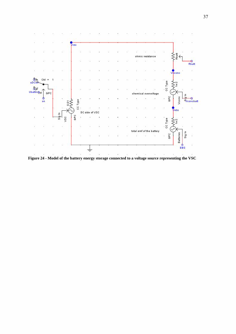
37

Figure 24 - Model of the battery energy storage connected to a voltage source representing the VSC

38

emf

chemical overvoltage

ohmic resistance

VSC DC voltage

battery voltage

Voltage control scheme

battery current

set power

Current limiting control

scheme

Calculation of SOC and emfinitial

SOC

SOC

emf

Calculation of ohmic resistance

battery temperature

battery age

reference DC voltage

Calculation of chemical

overvoltage

Calculation of battery

temperatureinitial batterytemperature

chemical overvoltage

current limits

Figure 25 - Simplified block diagram of the controls implemented in the RTDS model

7 Model testing To investigate how well the results from the complete RTDS model correspond to the results from Simulink model, some tests were performed under different operational conditions. The results from the RTDS model were compared with the results from the Simulink model and some adjustments of parameters were made to improve the results.

7.1 Dimensioning of the RTDS model The energy storage of DynaPeaQ can be designed and dimensioned to fit the energy and power requirements for a certain unit. Several battery cells are connected in series to build up battery modules. These are in turn connected in series to form battery strings. A number of battery strings could be connected in parallel. The number of modules connected in series

39

determines the DC voltage of the energy storage, whereas the numbers of strings connected in parallel determine the power that can be delivered or absorbed [16]. The RTDS model, built up in RSCAD, was constructed to be design-independent. This means the model could be used for any DynaPeaQ design by simply adjusting some parameters of the battery matrix, like the number of strings and the number of modules per string. However, since the model was developed for the power cell type, the available energy, the state of charge and the maximum allowed current calculated during the RTDS simulation will not be correct for energy storage designs with middle range or high energy cell types. Even though the voltage and power ratings of the energy storage should not influence the performance of the model, it was decided that the testing of the model should be performed for a realistic design. A design made in a case study [18] concerning frequency regulation in the Finnish grid was chosen.

7.1.1 Frequency regulation design For a battery energy storage for frequency regulation applications, the aim is to keep the SOC level at approximately 50 %. Thus since the energy storage should be able to counteract positive as well as negative frequency deviations and hence needs capability to absorb as well as supply active power. The Finnish Transmission System Operator required a minimum power of 5 MW during 30 minutes, i.e. an energy capacity of 2.5 MWh. However, since the average SOC level should be 50 %, the design was made for the double energy capacity, 5 MWh. The medium range cells were used for this design. This cell type has a discharge power of 146 W when fully aged. Basing the design on this end of life–capacity gave a minimum requirement of 34 247 cells. In order to get identical battery strings and suitable values of DC voltage and current, the final design included 36 288 battery cells, building up two battery strings [18]. The same configuration was used for the testing of the RTDS model. Since the model is created for high power cells, the ratings were not the same as for the energy storage designed for the Finnish grid. In particular, an energy storage with high power cells could not provide the rated power for the entire rated time of an identically designed energy storage with medium range cells. On the other hand, it could provide or absorb more power during shorter time periods. Although using the above mentioned design for the RTDS model would not give a result that could be applied to the energy storage in the study [18], it was still concluded to be a realistic design even for an energy storage with high power cells and hence good enough for the testing purpose.

7.2 Simulation setup The RTDS model was run and evaluated in the test area at ABB FACTS, where all RTDS racks are situated. As no control systems that will communicate with the DynaPeaQ battery energy storage were available, the model could not be tested with the real control equipment. Instead, all controls necessary for the testing were implemented in RSCAD. This made the setup of the testing very simple, as no hardware needed to be connected to the RTDS rack. As soon as the model, built in RSCAD, had been compiled on the right rack, the model could be run from RSCAD/Runtime on the PC connected to the rack. The rack used was rack 2. For the simulations, a time step of 100 μs was used.

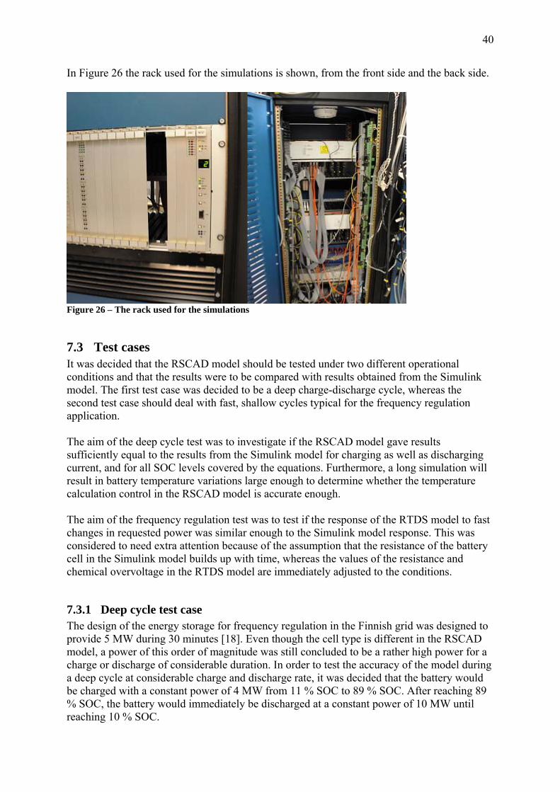
40

In Figure 26 the rack used for the simulations is shown, from the front side and the back side.

Figure 26 – The rack used for the simulations

7.3 Test cases It was decided that the RSCAD model should be tested under two different operational conditions and that the results were to be compared with results obtained from the Simulink model. The first test case was decided to be a deep charge-discharge cycle, whereas the second test case should deal with fast, shallow cycles typical for the frequency regulation application. The aim of the deep cycle test was to investigate if the RSCAD model gave results sufficiently equal to the results from the Simulink model for charging as well as discharging current, and for all SOC levels covered by the equations. Furthermore, a long simulation will result in battery temperature variations large enough to determine whether the temperature calculation control in the RSCAD model is accurate enough. The aim of the frequency regulation test was to test if the response of the RTDS model to fast changes in requested power was similar enough to the Simulink model response. This was considered to need extra attention because of the assumption that the resistance of the battery cell in the Simulink model builds up with time, whereas the values of the resistance and chemical overvoltage in the RTDS model are immediately adjusted to the conditions.

7.3.1 Deep cycle test case The design of the energy storage for frequency regulation in the Finnish grid was designed to provide 5 MW during 30 minutes [18]. Even though the cell type is different in the RSCAD model, a power of this order of magnitude was still concluded to be a rather high power for a charge or discharge of considerable duration. In order to test the accuracy of the model during a deep cycle at considerable charge and discharge rate, it was decided that the battery would be charged with a constant power of 4 MW from 11 % SOC to 89 % SOC. After reaching 89 % SOC, the battery would immediately be discharged at a constant power of 10 MW until reaching 10 % SOC.

41

The reason for choosing a higher power during discharge than during charge is that the battery cells can endure higher currents during discharge, and thus a higher power can be delivered. The charge power chosen, 4 MW, was close to the maximum power that could be charged at low SOC levels, when the voltage is low and the current therefore high, without endangering the charge current limit. The interval 10-90 % SOC is the operational range for which the RTDS model has been implemented. The intention was to test the entire SOC range of the model, but the very limits were excluded from the testing. Thus in order to have some margin to the model limits and avoid possible difficulties with determining when to stop charging, in order not to get outside the operational range. To get a reference, the Simulink model was run. In order to obtain the requested power at battery cell level, the 4 MW charge power and the 10 MW discharge power was divided between the 36 288 battery cells of the chosen design. This resulted in a charge power of 110.2293 W and a discharge power of 275.5732 W. A charging was performed for the single cell in the Simulink model. Starting at 11 % SOC and running the simulation until the battery was fully charged, the time elapsed between 11 and 89 % SOC was easily obtained. A simple control was implemented in the Simulink model, to switch the set power from 110.2293 W (charge) to -275.5732 W (discharge) after this time. The SOC, terminal voltage and temperature of the battery cell versus time were then recorded, to be used for verification of the RTDS model. The RTDS test was run under two different conditions: new batteries with initial battery temperature and ambient temperature 25°C and fully aged batteries with initial battery temperature and ambient temperature 20°C. However, in the test for aged batteries the charge was only performed until the SOC level reached approximately 80 %. The reason for this was to avoid violation of the voltage limits. The current ramping at high or low SOC levels were excluded from the model during these tests, since this control would have made the comparison with the Simulink results more difficult. Thus since the power asked for would not be the power actually delivered by the RTDS model if the current ramping control were used. However, the current ramping control for high and low terminal voltage was used. It turned out that it would act towards the end of the charge period, which would cause a small difference in SOC between the RTDS model and the Simulink model during this part of the test cycle.

7.3.2 Frequency regulation test case For the above mentioned study [18], the Finnish Transmission System Operator provided frequency data for 11 weeks distributed over one year. When the grid frequency deviated more than ± 0.05 Hz from 50 Hz the energy storage should be charged or discharged, respectively, to counteract the deviations. Moreover, when the frequency is inside this deadband, i.e. between 49.95 Hz and 50.05 Hz, the batteries should be charged if the SOC level is too low and discharged if the SOC level is too high. Thus the SOC level should be kept close to 50 % in order to be able to perform regulation of positive as well as negative frequency deviations. These two criteria were implemented as controls, and through simulations the power to be absorbed or provided by the energy storage over time was obtained [18]. For the testing of the RTDS model, it was decided that ten minutes of frequency regulation would be sufficient. A section of power versus time data of ten minutes duration was taken

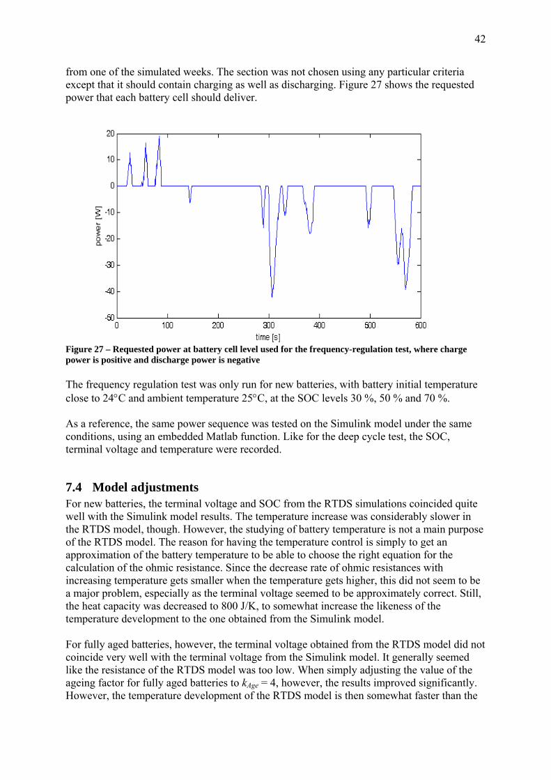
42

from one of the simulated weeks. The section was not chosen using any particular criteria except that it should contain charging as well as discharging. Figure 27 shows the requested power that each battery cell should deliver.

Figure 27 – Requested power at battery cell level used for the frequency-regulation test, where charge power is positive and discharge power is negative The frequency regulation test was only run for new batteries, with battery initial temperature close to 24°C and ambient temperature 25°C, at the SOC levels 30 %, 50 % and 70 %. As a reference, the same power sequence was tested on the Simulink model under the same conditions, using an embedded Matlab function. Like for the deep cycle test, the SOC, terminal voltage and temperature were recorded.

7.4 Model adjustments For new batteries, the terminal voltage and SOC from the RTDS simulations coincided quite well with the Simulink model results. The temperature increase was considerably slower in the RTDS model, though. However, the studying of battery temperature is not a main purpose of the RTDS model. The reason for having the temperature control is simply to get an approximation of the battery temperature to be able to choose the right equation for the calculation of the ohmic resistance. Since the decrease rate of ohmic resistances with increasing temperature gets smaller when the temperature gets higher, this did not seem to be a major problem, especially as the terminal voltage seemed to be approximately correct. Still, the heat capacity was decreased to 800 J/K, to somewhat increase the likeness of the temperature development to the one obtained from the Simulink model. For fully aged batteries, however, the terminal voltage obtained from the RTDS model did not coincide very well with the terminal voltage from the Simulink model. It generally seemed like the resistance of the RTDS model was too low. When simply adjusting the value of the ageing factor for fully aged batteries to kAge = 4, however, the results improved significantly. However, the temperature development of the RTDS model is then somewhat faster than the

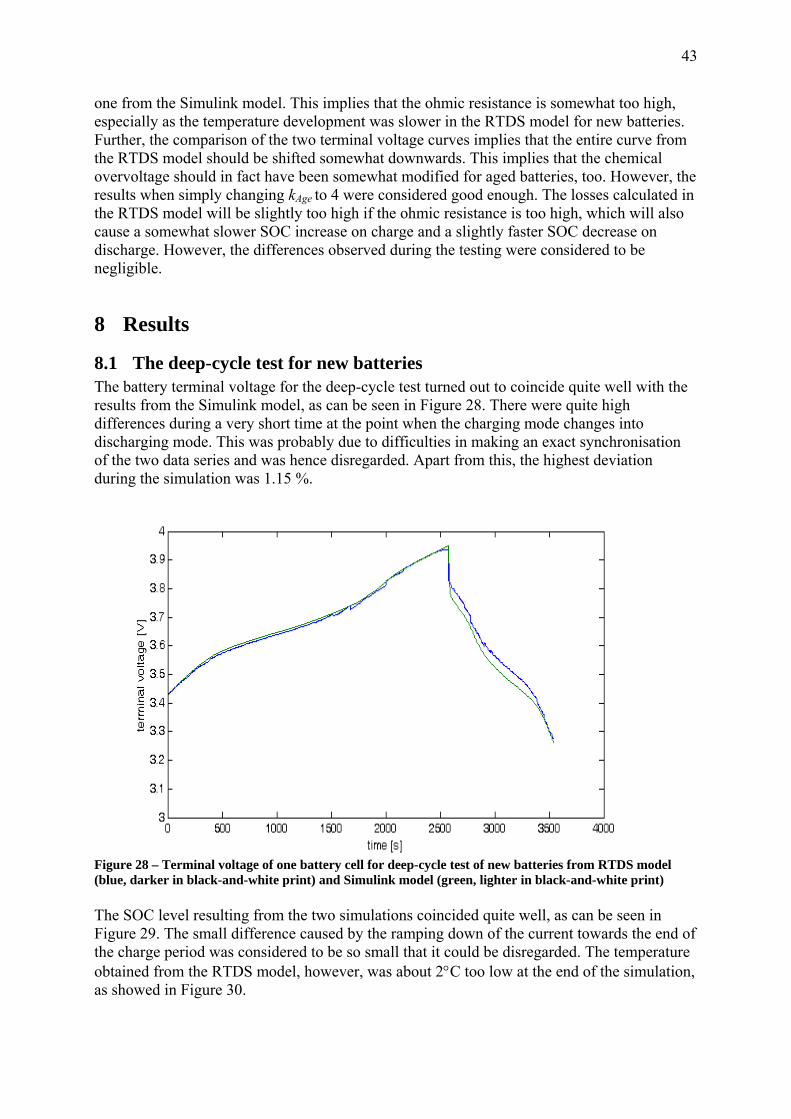
43

one from the Simulink model. This implies that the ohmic resistance is somewhat too high, especially as the temperature development was slower in the RTDS model for new batteries. Further, the comparison of the two terminal voltage curves implies that the entire curve from the RTDS model should be shifted somewhat downwards. This implies that the chemical overvoltage should in fact have been somewhat modified for aged batteries, too. However, the results when simply changing kAge to 4 were considered good enough. The losses calculated in the RTDS model will be slightly too high if the ohmic resistance is too high, which will also cause a somewhat slower SOC increase on charge and a slightly faster SOC decrease on discharge. However, the differences observed during the testing were considered to be negligible.

8 Results

8.1 The deep-cycle test for new batteries The battery terminal voltage for the deep-cycle test turned out to coincide quite well with the results from the Simulink model, as can be seen in Figure 28. There were quite high differences during a very short time at the point when the charging mode changes into discharging mode. This was probably due to difficulties in making an exact synchronisation of the two data series and was hence disregarded. Apart from this, the highest deviation during the simulation was 1.15 %.

Figure 28 – Terminal voltage of one battery cell for deep-cycle test of new batteries from RTDS model (blue, darker in black-and-white print) and Simulink model (green, lighter in black-and-white print) The SOC level resulting from the two simulations coincided quite well, as can be seen in Figure 29. The small difference caused by the ramping down of the current towards the end of the charge period was considered to be so small that it could be disregarded. The temperature obtained from the RTDS model, however, was about 2°C too low at the end of the simulation, as showed in Figure 30.

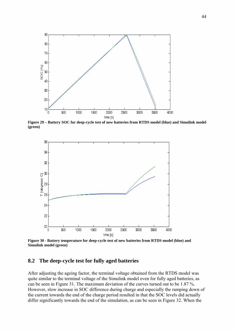
44

Figure 29 – Battery SOC for deep-cycle test of new batteries from RTDS model (blue) and Simulink model (green)

Figure 30 - Battery temperature for deep-cycle test of new batteries from RTDS model (blue) and Simulink model (green)

8.2 The deep-cycle test for fully aged batteries After adjusting the ageing factor, the terminal voltage obtained from the RTDS model was quite similar to the terminal voltage of the Simulink model even for fully aged batteries, as can be seen in Figure 31. The maximum deviation of the curves turned out to be 1.87 %. However, slow increase in SOC difference during charge and especially the ramping down of the current towards the end of the charge period resulted in that the SOC levels did actually differ significantly towards the end of the simulation, as can be seen in Figure 32. When the

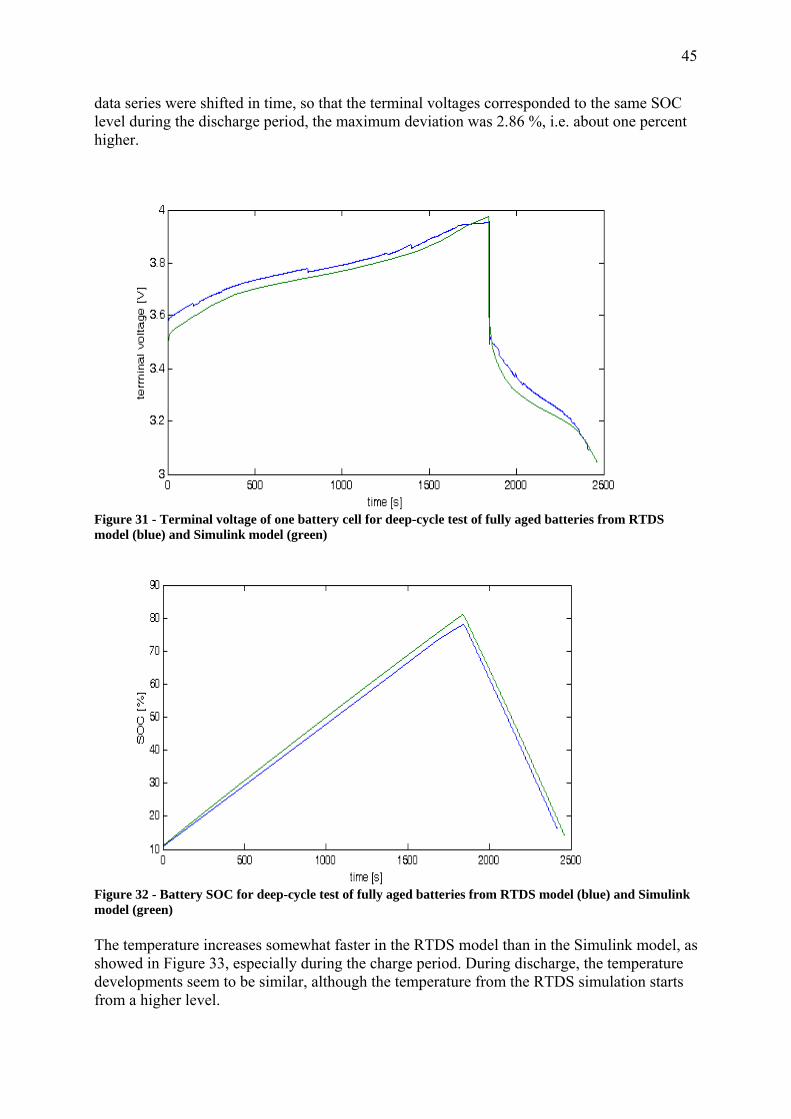
45

data series were shifted in time, so that the terminal voltages corresponded to the same SOC level during the discharge period, the maximum deviation was 2.86 %, i.e. about one percent higher.

Figure 31 - Terminal voltage of one battery cell for deep-cycle test of fully aged batteries from RTDS model (blue) and Simulink model (green)

Figure 32 - Battery SOC for deep-cycle test of fully aged batteries from RTDS model (blue) and Simulink model (green) The temperature increases somewhat faster in the RTDS model than in the Simulink model, as showed in Figure 33, especially during the charge period. During discharge, the temperature developments seem to be similar, although the temperature from the RTDS simulation starts from a higher level.

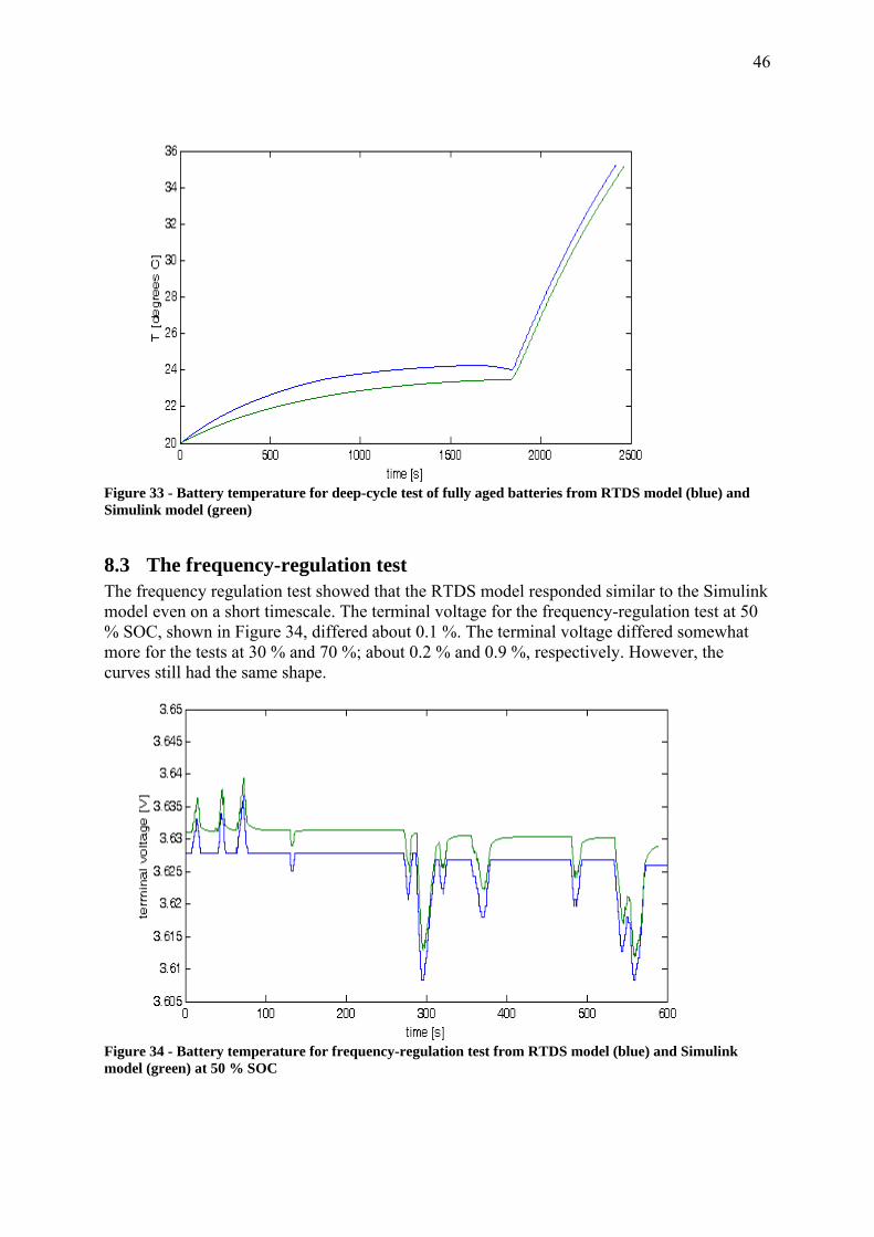
46

Figure 33 - Battery temperature for deep-cycle test of fully aged batteries from RTDS model (blue) and Simulink model (green)

8.3 The frequency-regulation test The frequency regulation test showed that the RTDS model responded similar to the Simulink model even on a short timescale. The terminal voltage for the frequency-regulation test at 50 % SOC, shown in Figure 34, differed about 0.1 %. The terminal voltage differed somewhat more for the tests at 30 % and 70 %; about 0.2 % and 0.9 %, respectively. However, the curves still had the same shape.

Figure 34 - Battery temperature for frequency-regulation test from RTDS model (blue) and Simulink model (green) at 50 % SOC

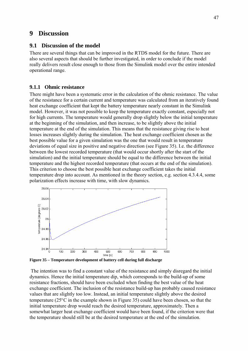
47

9 Discussion

9.1 Discussion of the model There are several things that can be improved in the RTDS model for the future. There are also several aspects that should be further investigated, in order to conclude if the model really delivers result close enough to those from the Simulink model over the entire intended operational range.

9.1.1 Ohmic resistance There might have been a systematic error in the calculation of the ohmic resistance. The value of the resistance for a certain current and temperature was calculated from an iteratively found heat exchange coefficient that kept the battery temperature nearly constant in the Simulink model. However, it was not possible to keep the temperature exactly constant, especially not for high currents. The temperature would generally drop slightly below the initial temperature at the beginning of the simulation, and then increase, to be slightly above the initial temperature at the end of the simulation. This means that the resistance giving rise to heat losses increases slightly during the simulation. The heat exchange coefficient chosen as the best possible value for a given simulation was the one that would result in temperature deviations of equal size in positive and negative direction (see Figure 35). I.e. the difference between the lowest recorded temperature (that would occur shortly after the start of the simulation) and the initial temperature should be equal to the difference between the initial temperature and the highest recorded temperature (that occurs at the end of the simulation). This criterion to choose the best possible heat exchange coefficient takes the initial temperature drop into account. As mentioned in the theory section, e.g. section 4.3.4.4, some polarization effects increase with time, with slow dynamics.

Figure 35 – Temperature development of battery cell during full discharge The intention was to find a constant value of the resistance and simply disregard the initial dynamics. Hence the initial temperature dip, which corresponds to the build-up of some resistance fractions, should have been excluded when finding the best value of the heat exchange coefficient. The inclusion of the resistance build-up has probably caused resistance values that are slightly too low. Instead, an initial temperature slightly above the desired temperature (25°C in the example shown in Figure 35) could have been chosen, so that the initial temperature drop would reach the desired temperature, approximately. Then a somewhat larger heat exchange coefficient would have been found, if the criterion were that the temperature should still be at the desired temperature at the end of the simulation.

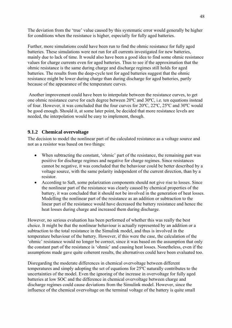
48

The deviation from the ‘true’ value caused by this systematic error would generally be higher for conditions when the resistance is higher, especially for fully aged batteries. Further, more simulations could have been run to find the ohmic resistance for fully aged batteries. These simulations were not run for all currents investigated for new batteries, mainly due to lack of time. It would also have been a good idea to find some ohmic resistance values for charge currents even for aged batteries. Thus to see if the approximation that the ohmic resistance is the same during charge and discharge regimes still holds for aged batteries. The results from the deep-cycle test for aged batteries suggest that the ohmic resistance might be lower during charge than during discharge for aged batteries, partly because of the appearance of the temperature curves. Another improvement could have been to interpolate between the resistance curves, to get one ohmic resistance curve for each degree between 20ºC and 30ºC, i.e. ten equations instead of four. However, it was concluded that the four curves for 20ºC, 22ºC, 25ºC and 30ºC would be good enough. Should it, at some later point, be decided that more resistance levels are needed, the interpolation would be easy to implement, though.

9.1.2 Chemical overvoltage The decision to model the nonlinear part of the calculated resistance as a voltage source and not as a resistor was based on two things:

• When subtracting the constant, ‘ohmic’ part of the resistance, the remaining part was positive for discharge regimes and negative for charge regimes. Since resistances cannot be negative, it was concluded that the behaviour could be better described by a voltage source, with the same polarity independent of the current direction, than by a resistor.

• According to Saft, some polarization components should not give rise to losses. Since the nonlinear part of the resistance was clearly caused by chemical properties of the battery, it was concluded that it should not be involved in the generation of heat losses. Modelling the nonlinear part of the resistance as an addition or subtraction to the linear part of the resistance would have decreased the battery resistance and hence the heat losses during charge and increased them during discharge.

However, no serious evaluation has been performed of whether this was really the best choice. It might be that the nonlinear behaviour is actually represented by an addition or a subtraction to the total resistance in the Simulink model, and thus is involved in the temperature behaviour of the battery. However, if this were the case, the calculation of the ‘ohmic’ resistance would no longer be correct, since it was based on the assumption that only the constant part of the resistance is ‘ohmic’ and causing heat losses. Nonetheless, even if the assumptions made gave quite coherent results, the alternatives could have been evaluated too. Disregarding the moderate differences in chemical overvoltage between different temperatures and simply adopting the set of equations for 25ºC naturally contributes to the uncertainties of the model. Even the ignoring of the increase in overvoltage for fully aged batteries at low SOC and the difference in chemical overvoltage between charge and discharge regimes could cause deviations from the Simulink model. However, since the influence of the chemical overvoltage on the terminal voltage of the battery is quite small

49

compared to the influence of the ohmic resistance for most SOC levels, these simplifications were considered to be justified, in order to keep the model reasonably simple.

9.1.3 Temperature calculations When developing the model, it was assumed that the only process generating heat within the battery was the heat losses caused by the ohmic resistance. Other possible sources of heating, like heat generation due to phase changes or changes in heat capacity, were completely ignored. However, according to [41] such a simplification should not have a major impact on the model accuracy. It could also be reasoned that possible extra sources of heating would already have been accounted for when determining the heat capacity: If extra sources of heat were present in the Simulink model, the calculated value of the heat capacity would be slightly lower than the ‘true’ value. This does not seem to be the case, though. Rather the initially calculated heat capacity seemed to be too high and needed to be reduced in order to produce a temperature development similar to the one produced by the Simulink model. This could on the other hand also be caused by errors in the implementation of the temperature calculations in RTDS. Generally, the most important factors for the temperature evolution during a charge/discharge cycle are probably the ohmic resistance and the heat capacity, together with the ambient temperature. The terminal voltage correctness could also have a significant impact, since a too high terminal voltage will result in a lower current and vice versa and the heating of the battery is directly proportional to the square of the current. The partial adjustment of the temperature development by simply changing the heat capacity was decided to be justified, even if it means that the temperature calculations are no longer directly based on the investigation of the Simulink model. Thus since the main purpose of the model is not to study thermal properties of the battery.

9.1.4 SOC calculations The calculation of SOC in the RTDS model is based on the assumption that the capacity of the battery remains the same, apart from reductions due to ageing. However, according to the Simulink model, the capacity is somewhat reduced at temperatures below 25 degrees. As this capacity decrease is only of about one percent, it was decided that the discrepancy could be disregarded. The error due to this simplification should probably be much smaller than the ones caused by several other sources of uncertainty. The Simulink model is based on a minimum capacity high power battery cell of 27.3 Ah. To test the agreement of the RTDS model with the Simulink model it was therefore necessary to define the capacity of the batteries in the energy storage as the minimum capacity too. Thus since using the average battery capacity, 30 Ah, in the RTDS model would have resulted in different SOC evolution for the same charge or discharge cycles in the RTDS model and the Simulink model, which would, in turn, significantly impact the battery terminal voltage. This naturally means that the results from the RTDS simulations represent an extreme worst case situation. Since 30 Ah is the average capacity, it is of course the value that should be used for an energy storage of over 30 000 batteries, if the aim were to obtain realistic results. Hence, the results obtained should not be seen as representative of a physical energy storage, but only as a means to evaluate the correctness of the RTDS model compared to the Simulink model.

50

It is very simple, though, to change the capacity of the batteries in the RTDS model, by simply changing the value on a slider to 30 Ah. After some reasoning, it was concluded that everything else in the model should still hold, even if the battery capacity is changed. The only thing that could possibly be impacted is the OCV versus SOC curve. However, according to Saft the correspondence of OCV and SOC holds for all three battery cell types, even though the battery capacity varies between 30 Ah (for high power cells) and 45 Ah (for high energy cells). Since, consequently, a difference in capacity of 15 Ah does not make a difference, the capacity difference of 2.7 Ah between average and minimum capacity high power cells should not impact the correspondence of OCV and SOC either.

9.2 Discussion of results and improvements The terminal voltage of a battery cell obtained from the RTDS model does never deviate more than 3 % for the tests that have been run. This must be considered to be a good result, with all simplifications made when constructing the model in thought. However, there could of course be larger deviations for operational conditions not covered by the test cases. The SOC range and the temperature range can be considered as quite well covered by the test cases, but when it comes to current only some parts of the current range have been tested. Low currents could be considered to be covered by the frequency-regulation test, currents around 30 A are covered by the charge part of the deep-cycle test and currents between 70 A and 90 A are approximately covered by the discharge part of the deep-cycle test. However, for currents between 40 A and 60 A some testing should be performed. Most important would probably be to test the model at higher currents, though, since higher currents will make the voltage drop over an incorrectly sized resistance larger, and hence increase the differences compared to the Simulink model. The frequency regulation test shows that the RTDS model changes its terminal voltage approximately at the same rate as the Simulink model, when a certain power is requested. However, the fact that the requested power is quite low for the entire test sequence means that a possible initial deviation in resistance magnitude would not cause a major difference in the terminal voltages from the two models. The voltage drop over the internal battery resistance will be quite small for both models, due to the low currents flowing. Therefore, it could have been a good idea to choose a test sequence with higher requested amounts of power. The largest deviation in terminal voltage for the frequency regulation test was found for the test run at 70 % SOC. The voltage from the RTDS model was about 0.9 % lower than the voltage from the Simulink model. This could probably be explained by the fact that the chemical overvoltage is not zero when the current is zero. The error caused by the negative contribution to the terminal voltage from the chemical overvoltage at no current should be largest for 70 % SOC. Thus since the magnitude of the chemical overvoltage is largest for low currents at that SOC level (cf. Figure 20). (The chemical overvoltage actually gives a minor positive contribution to the terminal voltage at no current for 30 % SOC and 50 % SOC). This means that the worst possible case when it comes to this error has actually been tested. Since this worst-case simulation at 70 % SOC resulted in a deviation in voltage smaller than 1 %, the simplification of not forcing the chemical overvoltage to be zero when no current flows seems to be justified. The fact that the results for aged batteries improved significantly when the ageing factor was increased from 2.65 to 4, although the testing of the equations alone gave quite good correspondence with the Simulink model for kAge = 2.65, should be considered. When

51

studying the appearance of the terminal voltage curve for new batteries, the ohmic resistance seems to be somewhat too low, as the voltage from the RTDS model is lower than the voltage from the Simulink model during charge and higher than the voltage from the Simulink model during discharge. These deviations would be increased when the magnitude of the resistance is scaled up, since the voltage drop gets larger altogether. In that respect, it seems logical that the deviation for older batteries was larger, and the ageing factor hence needed to be increased to compensate for a too low resistance for new batteries. A slightly too low resistance could, as mentioned before, be caused by a systematic error when iteratively obtaining the resistance values from the Simulink model. This does not, however, explain why the equations themselves gave a better correspondence with the Simulink model than does the entire RTDS model. Some deviations might be caused by the computational algorithms within the RTDS hardware. The quantities of an electrical circuit in RTDS are computed as kilovolts and kiloamperes. The equations implemented to calculate the resistance and chemical overvoltage need the current in amperes as an input, though. The current obtained from the electrical circuit is hence transformed to amperes, the resistance for one single battery cell is computed and finally the total resistance of the BESS is summed up. During this computational process there might possibly be some rounding errors that could contribute to the deviation from the Simulink model results. Another possibility is of course that there could be an error in the implementation of the equations in RTDS. However, none has been found. The resemblance of the SOC curves is generally good, especially for new batteries. For aged batteries the difference is slightly larger between the RTDS results and the Simulink results. This is probably caused by the fact that the ohmic resistance is somewhat too large after the adjustment of the ageing factor made in order to get a better terminal voltage, and this naturally causes slightly increased losses. Still, the results can probably be concluded to be good enough, since the deviation in SOC is small. Further, the main purpose of the model is not to simulate the losses, even if it could deliver an approximation of the resistive losses. This approximation will be somewhat too high for aged batteries and could hence be seen as conservative. The temperature development does not show a perfect resemblance with the temperature from the Simulink model, even after the heat capacity adjustments. The part of the temperature calculation dealing with heat exchange with the surroundings seems to be quite correct. Thus since the temperature profiles coincide quite well when the current is insignificant during the simulation, i.e. for the frequency regulation test. Hence, the discrepancy between the curves when a current flows should be caused by the value of the ohmic resistance or the heat capacity. However, as long as the temperature simulated leads to a fairly correct terminal voltage, it should be acceptable. The resistance difference is smaller for higher temperatures, at least within the temperature range, which means that a difference of 2ºC in a temperature range close to 30ºC will not be important. Furthermore, as previously stated, the aim of the model is not to investigate the battery temperature.

9.2.1 Model limitations The decision to call the components representing the resistive behaviour of the battery ‘ohmic resistance’ and ‘chemical overvoltage’ might be misleading. As described in the theory section, the processes and phenomena causing battery polarization are numerous and complex. The approach in this master thesis work has been to find a model that can

52

reasonably well mimic the battery behaviour (or rather the behaviour of the Simulink model) within the operational range of the DynaPeaQ batteries, rather than creating a model where each component represents a chemical process or property. Thus, the ‘ohmic resistance’ of the RTDS model does not necessarily directly correspond to the ‘ohmic overvoltage’ described in the theory section and the ‘chemical overvoltage’ does not specifically correspond to any of the described overvoltages. Instead, the intention is that the ‘ohmic resistance’ should represent the share of the battery polarization that behaves like a resistance from an electrical point of view, independent on whether it is related to the transport of ions or electrons, diffusion phenomena or something else. I.e. it should follow Ohm’s law and cause heat losses equal to the resistance times the current squared. Similarly, the intention is that the ‘chemical overvoltage’ should account for the changes in battery terminal voltage that could not be explained by the ohmic resistance, no matter what chemical processes might have caused them. This modelling approach naturally brings with it that the components chosen to represent the battery behaviour in the RTDS model do not necessarily have any resemblance to the components inside the Simulink model. As long as the battery terminal voltage calculated by the RTDS model reasonably well coincides with the terminal voltage from the Simulink model this is not a problem. The aim of the RTDS model is not to simulate battery ageing or other internal battery properties, but rather to produce a correct voltage and power seen from the terminals where the energy storage will be connected to the SVC Light. However, it is important to emphasize that the RTDS model should only be used within the operational range for which it has been developed, since it might not behave like the Simulink model at all under other conditions. Further, one should keep in mind that the RTDS model is a model of a model, and not a model of real, measured battery behaviour. Unfortunately, testing of a real battery was not possible to perform within the frame of this master thesis work, but could be subject to future work.

10 Conclusion A battery energy storage model has been implemented in RTDS. Equations that can approximately calculate the battery resistance behaviour under different operational conditions have been obtained from simulations of the Simulink model. The battery terminal voltage obtained from the test simulations of the RTDS model reasonably well coincides with the results from the same test run on the Simulink model. Hence it is concluded that the RTDS model is good enough, at least for the operational conditions covered by the test simulations. However, some additional tests are probably needed.

11 Future work As mentioned in the discussion, more testing of the model is needed. Especially, the model should be tested for higher currents, if the intention is to use it for tests of the entire intended operational range of DynaPeaQ. This is probably the most important aspect to investigate further, but there are also other model properties that should be better evaluated. For example, the switching between different equations should be better tested, to ensure that the right value is really chosen at all points within the operational range. The current ramping related to terminal voltage limits could also be removed and the test cases run again, in order to really

53

test the terminal voltage close to these limits. Further, a new frequency-regulation test case with higher power peaks could be run. In order to improve the RTDS model, a more advanced model of the chemical overvoltage could be developed, that actually takes ageing and differences between charge and discharge into account. However, this would of course increase the complexity of the model. An investigation of how much the possible systematic error when obtaining the ohmic resistance is influencing the results could also be performed, to determine whether this error is significant enough to justify a recalculation of the ohmic resistances. In order to use the model for its intended application, the electrical circuit representing the BESS needs to be implemented in the small-time-step environment in RSCAD. Thus since the RTDS model of the SVC Light, to which the battery model is to be connected, is built in the small-time-step environment. Alternatively, an interface component that can connect the battery model operating in the normal-time-step environment to the SVC Light model operating in the small-time-step environment must be found. If none of these possible solutions are implementable, a third option could be to calculate the voltage at the BESS terminals by running the battery model in the normal-time-step environment. This voltage could then be imported to the small-time-step environment and used as input to a variable voltage source. This solution would however not include the resistive behaviour of the batteries in the main circuit model. The fact that the model has not been developed based on physical battery measurements is an obvious weakness. It would be very interesting to compare the model results with measurements of an actual battery cell or battery module. This could e.g. be done by running the same charge/discharge cycle for the model and the real battery, and evaluate how well the terminal voltages coincide. Such testing may be performed at a later stage, to evaluate how well the RTDS model corresponds to the reality.

54

References

[1] Tyll H K, Schettler F, Power System Problems solved by FACTS Devices, Power Systems Conference and Exposition, 2009

[2] Overbye T J, Weber J D, Visualizing the Electric Grid, IEEE Spectrum, vol. 38,

February 2001, p. 52-58

[3] Wu W, Wong C, FACTS Applications in Preventing Loop Flows in Interconnected Systems, IEEE Power Engineering Society General Meeting, July 2003

[4] Püttgen H B, MacGregor P R, Lambert F C, Distributed Generation: Semantic Hype

or the Dawn of a New Era?, IEEE Power & Energy Magazine, vol. 1, January/February 2003, p. 22-29

[5] Beaudin M, Zareipour H, Schellenberglabe A, Rosehart W, Energy storage for

mitigating the variability of renewable electricity sources: An updated review, Energy for Sustainable Development 14, 2010, p. 302-314

[6] Divya K C, Østergaard J, Battery energy storage technology for power systems – An

overview, Electric Power Systems Research 79, 2009, p. 511-520

[7] Link D, Wheelock C, Energy Storage on the Grid – Long Duration Energy Storage Systems: Compressed Air, Pumped Hydro, NAS Batteries, Flow Batteries, and Lithium Ion Batteries for Utility-Scale Storage, Research Report, Pike Research, 2010

[8] Acha E, Ambriz-Pérez H, Angeles-Camacho C, Fuerte-Esquivel C R, Facts :

Modelling and Simulation in Power Networks, Wiley, Chichester, 2004, ISBN 10: 0-470-85271-2 (WB) ISBN 13: 978-0-470-85271-2 (WB), p. 1-5, 28-34

[9] Mohan N, Undeland T M, Robbins W P, Power Electronics – Converters,

applications and design, Wiley, 2003, p. 202-208, 471-475

[10] Taylor C W, Power System Voltage Stability, McGraw-Hill, Singapore, 1994, p.42, 51-61

[11] Noroozian M, Petersson N A, Thorvaldson B, Nilsson A B, Taylor C W, Benefits of

SVC and STATCOM for electric utility application, 2003 IEEE PES Transmission and Distribution Conference and Exposition, 2004

[12] Østergaard P A, Transmission-grid requirements with scattered and fluctuating

renewable electricity-sources, Applied Energy 76, 2003, p. 247-255

[13] Yang Z, Shen C, Zhang L, Crow M L, Atcitty S, Integration of a StatCom and Battery Energy Storage, IEEE Transactions on Power Systems, vol. 16, no. 2, May 2001, p. 254-260

[14] Arulampalam A, Barnes M, Jenkins N, Ekanayake J B, Power quality and stability

improvement of a wind farm using STATCOM supported with hybrid battery energy

55

storage, IEE Proceedings – Generation, Transmission and Distribution, vol. 153, no.6, November 2006, p. 701-710

[15] ABB AB FACTS, SVC Light® with Energy Storage, ABB Id No A02-0211 E/01/10

[16] ABB AB FACTS, DynaPeaQ® SVC Light® with Energy Storage, ABB Id No A02-

0210 E, 2010

[17] Svensson J, Hermansson W, Dynamic Energy Storage using SVC Light, Cigre Session 42, 2008, B4-204

[18] Holmberg M T, Lahtinen M, Larsson T, McDowall J, SVC Light® with Energy

Storage for frequency regulation, 2010 IEEE Conference on Innovative Technologies for an Efficient and Reliable Electricity Supply (CITRES), November 2010

[19] Liu C C, Lu C F, Wu C J, Dynamic modelling of battery energy storage system and

application to power system stability, IEE Proceedings – Generation, Transmission and Distribution, vol. 142, no.4, July 1995, p. 429-435

[20] Kaiser R, Optimized battery-management system to improve storage lifetime in

renewable energy systems, Journal of Power Sources 168, 2007, p.58-65

[21] Tsang K M, Sun L, Chan W L, Identification and modelling of Lithium ion battery, Energy Conversion and Management 51, 2010, p. 2857-2862

[22] Ménard L (corresponding author), Fontès G, Astier S, Dynamic energy model of a

lithium-ion battery, Original article, Mathematics and Computers in Simulation 81, 2010, p. 327-339

[23] Barret J-P, Bornard P, Meyer B, Power System Simulation, first edition, Chapman &

Hall, Great Britain, 1997, ISBN 0 412 63870 3, p.

[24] Burns A, Wellings A, Real-Time Systems and Programming Languages, second edition, Addison-Wesley, Great Britain, 1996, ISBN 0-201-40365-X, p. 2-3, 33-34

[25] Kuffel R, Giesbrecht J, Maguire T, Wierckx R P, McLaren P, RTDS – A fully digital

power system simulator operating in real time, IEEE Catalogue No. 95TH8130, 1995, p. 498-503

[26] RTDS Hardware Manual, rev 00, RTDS Technologies, January 2009

[27] Real Time Digital Simulator - Power System Users Manual, RTDS Technologies,

November 2006, p. 1.5-1.7

[28] Svensson J, Grid-Connected Voltage Source Converter – Control Principles and Wind Energy Applications, Technical Report No. 331, School of electrical and computer engineering, Chalmers University of Technology, Göteborg, Sweden, 1998, p. 11-19, 43-44

56

[29] Yang Z, Shen C, Zhang L, Crow M L, Atcitty S, Integration of a StatCom and Battery Energy Storage, IEEE Transactions on Power Systems, vol. 16, no. 2, May 2001, p. 254-260

[30] Linden D (ed.), Reddy T B (ed.), Ehrlich G M, Handbook of batteries, third edition,

McGraw-Hill, 2002, USA, ISBN 0-07-135978-8, p. 35.1-35.5

[31] Sarre G, Blanchard P, Broussely M, Aging of lithium-ion batteries, Journal of Power Sources 127, 2004, p. 65-71

[32] Myland J C, Oldham K B (corresponding author), Polarization inventory diagrams,

Journal of Electroanalytical Chemistry 504, 2001, p. 137-145

[33] Dubarry M, Svoboda V, Hwu R, Liaw B Y (corresponding author), Capacity loss in rechargeable lithium cells during cycle life testing: The importance of determining state-of-charge, Journal of Power Sources 174, 2007, 1121-1125

[34] Nyman A, Zavalis T G, Elger R, Behm M, Lindbergh G, Analysis of the Polarization

in a Li-Ion Battery Cell by Numerical Simulations, Journal of the Electrochemical Society, 157 (11), September 2010, p. A1236-A1246

[35] Liaw B Y (corresponding author), Nagasubramanian G, Jungst R G, Doughty D H,

Modeling of lithium ion cells – A simple equivalent-circuit model approach, Solid State Ionics 175, 2004, p. 835-839

[36] Liaw B Y (corresponding author), Jungst R G, Nagasubramanian G, Case H L,

Doughty D H, Modeling capacity fade in lithium-ion cells, Journal of Power Sources 140, 2005, p. 157-161

[37] Atkins P, Jones L, Chemical Principles – The Quest for Insight, fourth edition, W. H.

Freeman and Company, USA, 2008, ISBN-13: 978-0-7167-7355-9, ISBN-10: 0-7167-7355-4, p. 556-561

[38] Dubarry M, Liaw B Y (corresponding author), Development of a universal modeling

tool for rechargeable lithium batteries, Journal of Power Sources 174, 2007, p. 856-860

[39] Dubarry M, Vuillaume N, Liaw B Y (corresponding author), From single cell model

to battery pack simulation for Li-ion batteries, Journal of Power Sources 186, 2009, p. 500-507

[40] Jim McDowall, Saft, oral communication, 9 March 2011

[41] Chen S X, Tseng K J, Choi S S, Modeling of Lithium-Ion Battery for Energy Storage

System Simulation, Power and Energy Engineering Conference, APPEEC, Asia-Pacific, 2009