Embed Size (px)
Citation preview

RS
, ©
200
4 C
arne
gie
Mel
lon
Uni
vers
ity
Training HMMs with shared parameters
Class 24, 18 apr 2012
RS
, ©
200
4 C
arne
gie
Mel
lon
Uni
vers
ity
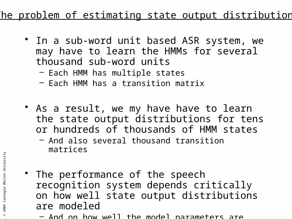
• In a sub-word unit based ASR system, we may have to learn the HMMs for several thousand sub-word units– Each HMM has multiple states– Each HMM has a transition matrix
• As a result, we my have have to learn the state output distributions for tens or hundreds of thousands of HMM states– And also several thousand transition matrices
• The performance of the speech recognition system depends critically on how well state output distributions are modeled– And on how well the model parameters are learned
The problem of estimating state output distributions

RS
, ©
200
4 C
arne
gie
Mel
lon
Uni
vers
ity
• The state output distributions might be anything in reality. We model these using various simple densities– Gaussian– Mixture Gaussian– Other exponential densities
• The models must be chosen such that their parameters can be easily estimated.– If the density model is inappropriate for the data, the HMM will be a poor statistical
model– Gaussians are imperfect models for the distribution of cepstral features
• Gaussians are very poor models for the distribution of power spectra• Empirically, the most effective model has been found to be the mixture
Gaussian density
Gaussian Mixture Gaussian Laplacian
Modeling state output distributions
actual distribution of data

RS
, ©
200
4 C
arne
gie
Mel
lon
Uni
vers
ity
• The parameters required to specify a mixture of K Gaussians includes K mean vectors, K covariance matrices, and K mixture weights– All of these must be learned from training data
• A recognizer with tens (or hundreds) of thousands of HMM states will require hundreds of thousands (or millions) of parameters to specify all state output densities– If state output densities are modeled by mixture Gaussians
• Most training corpora cannot provide sufficient training data to learn all these parameters effectively– Parameters for the state output densities of sub-word units that are
never seen in the training data can never be learned at all
The problem of estimating state output distributions

RS
, ©
200
4 C
arne
gie
Mel
lon
Uni
vers
ity
AO
To train the HMM for a sub-word unit, data from all instances of the unit in the training corpus are used to estimate the parameters
Transcript = FOX IN SOCKS ON BOX ON KNOX
F AO K S IH N S AO K S AO N B AO K S AO N N AO K S
Training models for a sound unit
IH EH

RS
, ©
200
4 C
arne
gie
Mel
lon
Uni
vers
ity
Gather data from separate instances, assign data to states, aggregate data for each state, and find the statistical parameters of each of the aggregates
Indiscriminate grouping of vectors of a unit from different locations in the corpus results in Context-Independent (CI) models
Training CI models for a sound unit
Schematic example of data usage for training a 5-state HMM
AO
HMM for the CI unit AO

RS
, ©
200
4 C
arne
gie
Mel
lon
Uni
vers
ity
Context based grouping of observations results in finer, Context-Dependent (CD) models
CD models can be trained just like CI models, if no parameter sharing is performed The number of subword units in a language
is usually very large
Usually insufficient training data to learn all subword HMMs properly (Typically subword units are triphones) Parameter estimation problems
Training sub-word unit models with shared parameters
• Parameter sharing is a technique by which several similar HMM states share a common set of HMM parameters
• Since the shared HMM parameters are now trained using the data from all the similar states, there are more data available to train any HMM parameter– As are result HMM parameters are well trained– This tradeoff is that the estimated parameters cannot discriminate between
the “tied” states

RS
, ©
200
4 C
arne
gie
Mel
lon
Uni
vers
ity
Sharing parameters
Individual states may share the same mixture distributions
unit1 unit2
Continuous density HMMs with tied states

RS
, ©
200
4 C
arne
gie
Mel
lon
Uni
vers
ity
Sharing parameters
Mixture Gaussian state densities: all states may share the same Gaussians, but with different mixture weights
unit1 unit2
Semi-continuous HMMs

RS
, ©
200
4 C
arne
gie
Mel
lon
Uni
vers
ity
Sharing parameters
unit1 unit2
Semi-continuous HMMs with tied states
Mixture Gaussian state densities: all states may share the same Gaussians, but with state-specific mixture weights, and then share the weights as well

RS
, ©
200
4 C
arne
gie
Mel
lon
Uni
vers
ity
• Partly a design choice– Semi-continuous HMMs, vs. phonetically tied-semi-continuous
HMMs vs. continuous density HMMs
• Automatic techniques– Data-driven Clustering
• Group HMM states together based on the similarity of their distributions, until all groups have sufficient data
– The densities used for grouping are poorly estimated in the first place– Has no estimates for unseen sub-word units– Places no restrictions on HMM topologies etc.
– Decision trees• Clustering based on expert-specified rules. The selection of rule is data
driven– Based on externally provided rules. Very robust if the rules are good– Provides a mechanism for estimating unseen sub-word units– Restricts HMM topologies
Deciding how parameters are shared
RS
, ©
200
4 C
arne
gie
Mel
lon
Uni
vers
ity
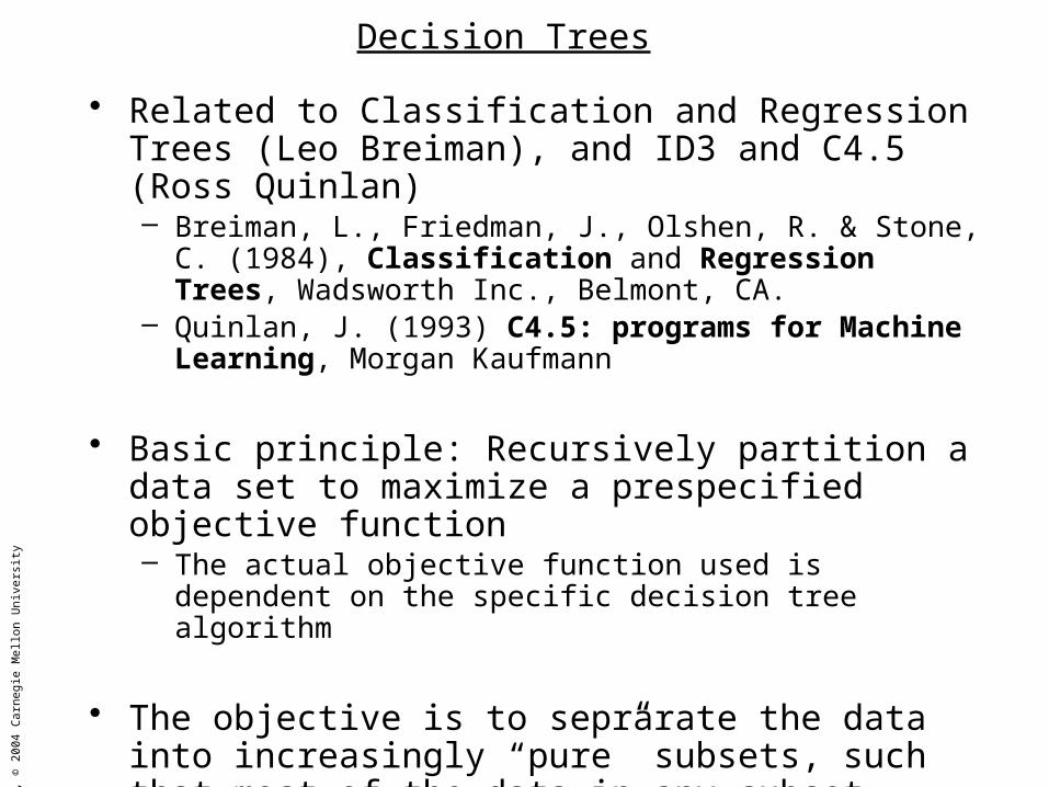
• Related to Classification and Regression Trees (Leo Breiman), and ID3 and C4.5 (Ross Quinlan)– Breiman, L., Friedman, J., Olshen, R. & Stone, C. (1984),
Classification and Regression Trees, Wadsworth Inc., Belmont, CA.– Quinlan, J. (1993) C4.5: programs for Machine Learning, Morgan
Kaufmann
• Basic principle: Recursively partition a data set to maximize a prespecified objective function– The actual objective function used is dependent on the specific
decision tree algorithm
• The objective is to seprarate the data into increasingly “pure” subsets, such that most of the data in any subset belongs to a single class– In our case the “classes” are HMM states
Decision Trees
RS
, ©
200
4 C
arne
gie
Mel
lon
Uni
vers
ity
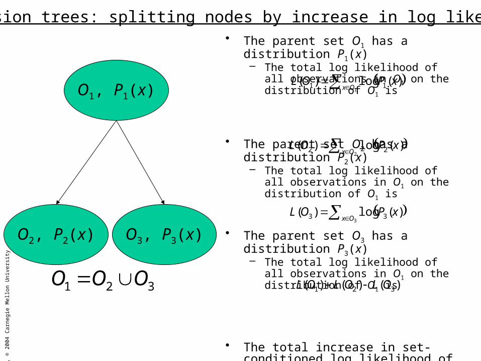
• The parent set O1 has a distribution P1(x)– The total log likelihood of all observations
in O1 on the distribution of O1 is
• The parent set O2 has a distribution P2(x)– The total log likelihood of all observations
in O1 on the distribution of O1 is
• The parent set O3 has a distribution P3(x)– The total log likelihood of all observations
in O1 on the distribution of O1 is
• The total increase in set-conditioned log likelihood of observations due to partitioning O1 is
• Partition O1 such that the increase in log likelihood is maximized– Recursive perform this partition of each of
the subsets to form a tree
Decision trees: splitting nodes by increase in log likelihood
O1, P1(x)
O2, P2(x) O3, P3(x)
321 OOO
1)(log)( 11 Ox
xPOL
2)(log)( 22 Ox
xPOL
3)(log)( 33 Ox
xPOL
)()()( 321 OLOLOL

RS
, ©
200
4 C
arne
gie
Mel
lon
Uni
vers
ity
• Identify set of states that can potentially be merged– Based on rules, rather than data, in order to enable prediction of
distributions of unseen sub-word units
• Partition the union of the data in all the states recursively using a decision tree procedure– Ensuring that entire states go together during the partitioning– Terminate the recursion at any leaf when partitioning the data at
the leaf will result in children with insufficient data for parameter estimation
– Alternately, grow the tree until each state is at a separate leaf, and prune the tree backwards until all leaves have sufficient data for parameter estimation
• The leaves of the resulting tree will include many states. All states in a leaf will share distribution parameters.
Decision trees for parameter sharing

RS
, ©
200
4 C
arne
gie
Mel
lon
Uni
vers
ity
A common heuristic is to permit states with identical indices in the HMMs for different N-phones for the same base phone to share parameters. E.g., the first state of all triphones of the kind
AA(*,*) are allowed to share distribution parameters
Within any index, states are be further clustered using a decision tree All states within each cluster share parameters In the worst case, where all N-phone states with
a common index share a common distribution results in simple CI phonemes
States with different indices are not allowed to share parameters
This heuristic enables the “synthesis” of HMMs for N-phones that were never seen in the training data This only works for N-phones for which base
phones can be identified
Heuristic for deciding which states can be grouped at the root of a tree
These states mayshare parameters
These states maynot share parameters

RS
, ©
200
4 C
arne
gie
Mel
lon
Uni
vers
ity
Each HMM state of every unseen N-phone is assumed to be clustered with some subset of states of the same index, that belong to other N-phones of the same base phone
The state output distribution for each HMM state of the unseen Nphone is set to be identical to the distribution for the cluster it belongs to
Estimating HMMs for unseen Nphones simply involves identifying the state clusters that their states belong to The clusters are identified based on
expert-specified rules
For this technique to work, the HMMs for all Nphones of a given basephone must have identical numbers of states and identical topologies
Synthesizing HMMs for unseen subword units
HMMs for seensubword units
HMM for unseen subword unit. The state output distribution for any state is identical to the distribution of a cluster of observed states
All N-phones with a common basephone are assumed to have identical transition matrices

RS
, ©
200
4 C
arne
gie
Mel
lon
Uni
vers
ity
All states with a common index are initially grouped together at the root node
Each node is then recursively partitioned
All states in the leaves of the decision tree share parameters
A separate decision tree is built for every state index for every base phone
The decision tree procedure attempts to maximize the loglikelihood of the training data
The expected log-likelihood of a vector drawn from a Gaussian distribution with mean m and variance C isThe assignment of vectors to states
can be done using previously trainedCI models or with CD models that havebeen trained without parameter sharing
)()(5.0 1
||)2(
1log
xCx
d
T
eC
E
Clustering states with decision trees

RS
, ©
200
4 C
arne
gie
Mel
lon
Uni
vers
ity
This is a function only of the variance of the Gaussian The expected log-likelihood of a set of N vectors is
)()(5.0 1
||)2(
1log
xCx
d
T
eC
E
||)2(log5.0)()(5.0 1 CxCxE dT
||)2(log5.0)()(5.0 1 CExCxE dT
||)2(log5.05.0 Cd d
||)2(log5.05.0 CNNd d
Expected log-likelihood of a vector drawn from a Gaussian distribution
Expected log-likelihood of a Gaussian random vector

RS
, ©
200
4 C
arne
gie
Mel
lon
Uni
vers
ity
||)2(log5.0||)2(log5.0||)2(log5.0 2211 CNCNCN ddd
||)2(log5.05.0||)2(log5.05.0 222111 CNdNCNdN dd
If we partition a set of N vectors with mean m and variance C into two sets of vectors of size N1 and N2 , with means m1 and m2 and variances C1 and C2 respectively, the total expected log-likelihood of the vectors after splitting becomes
The total log-likelihood has increased by
Observation vectors are partitioned into groups to maximize within class likelihoods
Partitioning each node of the decision tree

RS
, ©
200
4 C
arne
gie
Mel
lon
Uni
vers
ity
Ideally, every possible partition of vectors into two clusters must be evaluated
Partitioning each node of the decision tree
Partitioning is performed such that all vectors belonging to a single Nphone must together

RS
, ©
200
4 C
arne
gie
Mel
lon
Uni
vers
ity
Ideally, every possible partition of vectors into two clusters must be evaluated
Partitioning each node of the decision tree
Partitioning is performed such that all vectors belonging to a single Nphone must together

RS
, ©
200
4 C
arne
gie
Mel
lon
Uni
vers
ity
Ideally, every possible partition of vectors into two clusters must be evaluated
Partitioning each node of the decision tree
Partitioning is performed such that all vectors belonging to a single Nphone must together

RS
, ©
200
4 C
arne
gie
Mel
lon
Uni
vers
ity
Ideally, every possible partition of vectors into two clusters must be evaluated
Partitioning each node of the decision tree
Partitioning is performed such that all vectors belonging to a single Nphone must together

RS
, ©
200
4 C
arne
gie
Mel
lon
Uni
vers
ity
Partitioning each node of the decision tree
Ideally, every possible partition of vectors into two clusters must be evaluated
Partitioning is performed such that all vectors belonging to a single Nphone must together

RS
, ©
200
4 C
arne
gie
Mel
lon
Uni
vers
ity
Ideally, every possible partition of vectors into two clusters must be evaluated, the partition with the maximum increase in log likelihood must be chosen
Partitioning each node of the decision tree
Partitioning is performed such that all vectors belonging to a single Nphone must together

RS
, ©
200
4 C
arne
gie
Mel
lon
Uni
vers
ity
Ideally, every possible partition of vectors into two clusters must be evaluated, the partition with the maximum increase in log likelihood must be chosen, and the procedure must be recursively continued until a complete tree in built
The trees will have a large number of leaves
All trees must then be collectively pruned to retain only the desired number of leaves. Each leaf represents a tied state (sometimes called a senone)
All the states within a leaf share distribution parameters. The shared distribution parameters are estimated from all the data in all the states at the leaf
Partitioning each node of the decision tree
Partitioning is performed such that all vectors belonging to a single Nphone must together

RS
, ©
200
4 C
arne
gie
Mel
lon
Uni
vers
ity
2n-1 possible partitions for n vector groups. Exhaustive evaluation too expensive
Linguistic questions are used to reduce the search space
Linguistic questions are pre-defined phone classes. Candidate partitions are based on whether a context belongs to the phone class or not Example:
Sharing parameters: evaluating the partitions
Class1 EY EH IY IH AX AA R W N V ZClass2 F Z SH JH ZHClass3 T D K P BClass4 UW UH OW R W AYClass5 TH S Z V FClass6 IH IY UH UWClass7 W V FClass8 T KClass9 R W…

RS
, ©
200
4 C
arne
gie
Mel
lon
Uni
vers
ity
• Partitions are derived based only on answers to linguistic questions such as:– Does the left context belong to “class1”– Does the right context belong to “class1”– Does the left context NOT belong to “class1”– Does the right context NOT belong to “class1”
• The set of possible partitions based on linguistic questions is restricted and can be exhaustively evaluated
• Linguistic classes group phonemes that share certain spectral characteristics, and may be expected to have similar effect on adjacent phonemes.– Partitioning based on linguistic questions imparts “expert
knowledge” to an otherwise data-driven procedure.
Partitioning with linguistic questions

RS
, ©
200
4 C
arne
gie
Mel
lon
Uni
vers
ity
Composing HMMs for unseen Nphones
Vowel?
Z or S?
• Every non-leaf node in the decision tree has a question associated with it– The question that was eventually used to partition the node
• The questions are linguistic questions– Since partitioning is exclusively performed with linguistic questions
• Even unseen Nphones can answer the questions– They can therefore be propagated to the leaves of the decision trees
• The state output distribution for any state of an unseen Nphone is obtained by propagating the Nphone to a leaf of the appropriate decision tree for its base phone– The output distribution for all the states in the leaf is also assigned to the unseen
state

RS
, ©
200
4 C
arne
gie
Mel
lon
Uni
vers
ity
Meaningful Linguistic Questions?
Left context: (A,E,I,Z,SH)
ML Partition: (A,E,I) (Z,SH)
(A,E,I) vs. Not(A,E,I)
(A,E,I,O,U) vs. Not(A,E,I,O,U)
A
E
I Z
SH
Linguistic questions must be meaningful in order to deal effectively with unseen triphones
Linguistic questions
Linguistic questions effectively substitute expert knowledge for information derived from data
For effective prediction of the distributions of unseen subword units, the linguistic questions must represent natural groupings of acoustic phenomena
(A,E,I,O,U) vs. Not (A,E,I,O,U) represents a natural grouping of phonemes. The other groupings are not natural.

RS
, ©
200
4 C
arne
gie
Mel
lon
Uni
vers
ity
• Train HMMs for all triphones (Nphones) in the training data with no sharing of parameters
• Use these “untied” HMM parameters to build decision trees– For every state of every base phone
• This stage of training is the “context-dependent untied training”
Context Dependent Untied (CD untied) training for building decision trees
Before decision trees are built, all these HMMs must be trained !

RS
, ©
200
4 C
arne
gie
Mel
lon
Uni
vers
ity
There are several ways of pruning a tree to obtain a given number of leaves(6 in this example)
Each leaf represents a cluster of triphone states that will share parameters. The leaves are called tied states or senones
Senones are building blocks for triphone HMMs. A 5-state HMM for a triphone will have 5 senones
Prining decision trees before state tying

RS
, ©
200
4 C
arne
gie
Mel
lon
Uni
vers
ity
• Final CD models are trained for the triphones using the tied states
• Training finer models: Train mixtures of Gaussians for each senone– All states sharing the senone inherit the entire mixture– Mixtures of many Gaussians are trained by iterative splitting of
Gaussians• Gaussian splitting is performed for continuous models
– Initially train single Gaussian state distributions– Split Gaussian with largest mixture weight by perturbing mean
vector and retrain– Repeat splitting until desired number of Gaussians obtained in the
Gaussian mixture state distributions
Context Dependent tied state (CD tied) models

RS
, ©
200
4 C
arne
gie
Mel
lon
Uni
vers
ity
• Ad-hoc sharing: sharing based on human decision– Semi-continuous HMMs – all state densities share the
same Gaussians– This sort of parameter sharing can coexist with the
more refined sharing described earlier.
Other forms of parameter sharing

RS
, ©
200
4 C
arne
gie
Mel
lon
Uni
vers
ity
– Update formulae are the same as before, except that the numerator and denominator for any parameter are also aggregated over all the states that share the parameter
s utterance ttutt
s utterance tttutt
k sxkPts
xsxkPts
),|(),(
),|(),(
s utterance t jtutt
s utterance ttutt
sxjPts
sxkPtskP
),|(),(
),|(),()(
s utterance ttutt
s utterance t
Tktkttutt
k sxkPts
xxsxkPtsC
),|(),(
))()(,|(),(
Mean of kth Gaussianof any state in the set of states Qthat share the kth Gaussian
Covariance of kth Gaussianof any state in the set of states Q that share the kth Gaussian
Mixture weight of kth Gaussianof any state in the set of states Q that share a Gaussian mixture
Baum-Welch with shared state parameters

RS
, ©
200
4 C
arne
gie
Mel
lon
Uni
vers
ity
0
0.05
0.1
0.15
0.2
1 2 3 4 5 6 7 8 9 10 11 12 13
Gaussian index
00.020.040.060.080.1
0.120.140.160.18
1 2 3 4 5 6 7 8 9 10 11 12 13
Gaussian index
0
0.05
0.1
0.15
0.2
1 2 3 4 5 6 7 8 9 10 11 12 13
Gaussian index
State Mixture Weight distributions

RS
, ©
200
4 C
arne
gie
Mel
lon
Uni
vers
ity
State Mixture Weight distributions
A (I,J)
A (K,L)
A (M,N)
Gaussian index1 2 …………………256
Co
un
tsGaussian index
1 2 …………………256C
ou
nts
Gaussian index1 2 …………………256
Co
un
ts
K1 K2 …………………K256Total Count for each index =
Gaussian index1 2 …………………256
Co
un
ts
Gaussian index1 2 …………………256
Pro
ba
bili
ties
P1 P2 …………………P256
+
+
+
Pi= Ki/Ktotal

RS
, ©
200
4 C
arne
gie
Mel
lon
Uni
vers
ity
State Mixture Weight distributions
K1 K2 …………………K256
Gaussian index (Ci)1 2 …………………256
Co
un
ts
Gaussian index1 2 …………………256
Pro
ba
bili
ties
P1 P2 …………………P256Pi= Ki/Ktotal
Likelihood of getting the particular set of observations =
probability of getting C1, K1 times and
Probability of getting C2, K2 times and
….
Probability of getting C256, K256 times
256321 )()()()( 1111KKKK CPCPCPCP
i
Ki
iCP )(Taking logarithm of we get

RS
, ©
200
4 C
arne
gie
Mel
lon
Uni
vers
ity
State Mixture Weight distributions
K1 K2 …………………K256
Gaussian index (Ci)1 2 …………………256
Co
un
ts
Gaussian index1 2 …………………256
Pro
ba
bili
ties
P1 P2 …………………P256Pi= Ki/Ktotal
Likelihood of getting the particular set of observations =
i
Ki
iCP )(Taking logarithm of we get
)(log ii
i CPK
Normalizing over all data points Ktotal : i
iiii total
i CPCPCPK
K)(log)()(log
This is the entropy of the joint distribution of all states
RS
, ©
200
4 C
arne
gie
Mel
lon
Uni
vers
ity
State Mixture Weight distributions
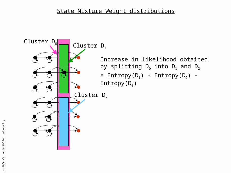
Increase in likelihood obtained by splitting D0 into D1 and D2
= Entropy(D1) + Entropy(D2) - Entropy(D0)
Cluster D1
Cluster D2
Cluster D0
RS
, ©
200
4 C
arne
gie
Mel
lon
Uni
vers
ity
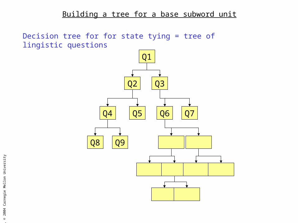
Building a tree for a base subword unit
Decision tree for for state tying = tree of lingistic questions
Q1
Q2 Q3
Q4 Q5 Q6 Q7
Q8 Q9

RS
, ©
200
4 C
arne
gie
Mel
lon
Uni
vers
ity
ss
sss
g N
NM
NNN
NMNMNMM
1173
11117733
Building decision trees for continuous density HMMs
A (I,J)
A (K,L)
A (M,N)
For each state, all data are comined to computed the state’s:
1) Total observation count (Ns)
2) Mean vector (Ms)
3) Covariance matrix (Cs)
1
5
9
2
8
10
3
9
11
4
9
14
ss
N
iis
ss CMx
Nx
s
2
1
2)(
2 1 s
sss
N
iis
N
iig xN
Nx
Nxx
ss2
1
2)(
1
22 11
22ggg MxC
The global mean of the union of the states
The global second moment
The global covariance

RS
, ©
200
4 C
arne
gie
Mel
lon
Uni
vers
ity
• The log likelihood of set of N vectors {O1, O2, …,ON }, as given by a Gaussian with mean M and covariance C is
Building decision trees for continuous density HMMs
N
iiN CMOGaussianOOOP
121 ),|( log),...,,(log
• The actual vectors are usually not recorded in an acoustic model. However, the number of vectors N in any state is usually known
• Approximate the total log likelihood for the set of observation with its expectation.
),|( log.),...,,(log 21 CMOGaussianENOOOP N
• This is N times the entropy of a variable O with a Gaussian distribution with mean M and covariance C

RS
, ©
200
4 C
arne
gie
Mel
lon
Uni
vers
ity
• Of all possible splits of the set of Ng vectors into a two sets of size N1 and N2, one maximizes the increase in log likelihood
• Select the split that maximizes the increase in log likelihood
Building decision trees for continuous density HMMs
D0
D1 D2
N2 Entropy(Gaussian(O | M2,C2))
• Increase in log likelihood:
),|( ..),|( ..),|( .. 222111 CMOGaussianEntNCMOGaussianEntNCMOGaussianEntN ggg
N1 Entropy(Gaussian(O | M1,C1))
Ng Entropy(Gaussian(O | Mg,Cg))