HSEHealth & Safety

Executive

Cost effective structural monitoring -

An acoustic method, phase IIb

Prepared by Mecon Ltd for the Health and Safety Executive 2005

RESEARCH REPORT 326

HSEHealth & Safety

Executive

Cost effective structural monitoring -

An acoustic method, phase IIb

Mecon Ltd5a Pound Hill

CambridgeCB3 0AE

This project is aimed at using long-range propagation of acoustic signals through at structure to detectchanges induced by damage, cracking or flooding of hollow members. It is based on the idea that, if achange occurs within the structure, this will induce changes in acoustic signals transmitted betweentwo points on it. These changes will only occur after a certain time in the history of the signal, and thistime corresponds to the minimum travel time from the transmission point to the reception point via thepoint of damage. This minimum time will correspond to the fastesttravelling waves; under normalcircumstances these are longitudinal compression waves. Thus if one is able to model the point-to-point transmission times of longitudinal compression waves through the structure, and one measuresbetween sufficiently many points, it should be possible to locate damage by picking the times at whichdifferences start to appear.

This report and the work it describes were funded by the Health and Safety Executive (HSE). Itscontents, including any opinions and/or conclusions expressed, are those of the authors alone and donot necessarily reflect HSE policy.

HSE BOOKS

ii

© Crown copyright 2005

First published 2005

ISBN 0 7176 2985 6

All rights reserved. No part of this publication may bereproduced, stored in a retrieval system, or transmitted inany form or by any means (electronic, mechanical,photocopying, recording or otherwise) without the priorwritten permission of the copyright owner.

Applications for reproduction should be made in writing to: Licensing Division, Her Majesty's Stationery Office, St Clements House, 2-16 Colegate, Norwich NR3 1BQ or by e-mail to hmsolicensing@cabinet-office.x.gsi.gov.uk

1. SUMMARY ........................................................................................................ 1

2. PROJECT PROGRESS TO DATE.................................................................. 2

2.1. RIG CONSTRUCTION...................................................................................... 22.2. TRANSDUCERS .............................................................................................. 22.3. SIGNAL CONDITIONING & DATA COLLECTION ............................................. 4

3. NUMERICAL MODELLING .......................................................................... 4

4. CALIBRATING THE NUMERICAL MODEL AGAINST THE PHYSICAL MODEL ...................................................................................................................... 6

5. SIGNAL CHARACTERISTICS ...................................................................... 7

5.1. NUMERICAL MODEL RESULTS....................................................................... 75.2. PHYSICAL MODEL RESULTS.......................................................................... 8

6. DAMAGE LOCATION ALGORITHMS........................................................ 9

7. MAGNITUDE OF DIFFERENCE SIGNALS AND DETECTABILITY OF DAMAGE ................................................................................................................. 10

8. TOMOGRAPHIC GEOMETRY EXPERIMENTS..................................... 11

8.1. DAMAGE ON A VERTICAL LEG .................................................................... 11 8.2. DAMAGE ON A DIAGONAL STRUT ............................................................... 12

9. REFLECTION GEOMETRY EXPERIMENTS .......................................... 12

9.1. PRE-IMPROVEMENT EXPERIMENT ............................................................... 129.2. POST-IMPROVEMENT EXPERIMENT ............................................................. 13

10. EFFECT OF TOPSIDES ............................................................................ 13

11. CONCLUSIONS .......................................................................................... 15

12. THE NEXT STAGE .................................................................................... 16

iii

iv

1. SUMMARY This project is aimed at using long-range propagation of acoustic signals through an offshore jacket structure to detect changes induced by damage, cracking or flooding of hollow members.

In the first phase of this project the method was proved on a two-dimensional polycarbonate model with two main legs and four complex nodes. Results were very promising.

The second phase has tested the method on a three-dimensional plastic model representative of the complexity of an offshore rig. In part 1, acoustic sources were located at the top of the model and sensors were located near the bottom. Signals were transmitted from each source to every sensor. This is a similar approach to computer aided tomography as used in medical, seismic and industrial applications where direct access to the inside of the human body, an oil reservoir or a chemical reactor is not possible. Cracking at a joint was simulated by partially cutting through a member. Results demonstrated that the location of structural damage could be accurately imaged. Work carried out on part 1 of Phase II has been reported in a paper at the May 2002 meeting of the Structural Integrity Monitoring Network (May 22, University College London).

In the final part of the work, the receivers have been moved from the bottom of the model rig to the top, to simulate an arrangement in which all transducers (sources and sensors) are above the waterline. Results demonstrate that this arrangement (which we refer to as the “reflection geometry”) can locate structural damage more accurately than the tomographic geometry. However it is also more sensitive to the effects of changes of temperature in the plastic rig, creep in the glue used to join it, and timing jitter and sampling rate drift in the data recording equipment. We have taken steps to reduce these sources of error and shown that this leads to accurate location of damage.

The project now needs to move on to tests on a metal structure immersed in water, preferably at larger scale.

This report constitutes the final deliverable on this project.

1

2. PROJECT PROGRESS TO DATE This project is aimed at using long-range propagation of acoustic signals through at structure to detect changes induced by damage, cracking or flooding of hollow members. It is based on the idea that, if a change occurs within the structure, this will induce changes in acoustic signals transmitted between two points on it. These changes will only occur after a certain time in the history of the signal, and this time corresponds to the minimum travel time from the transmission point to the reception point via the point of damage. This minimum time will correspond to the fastest-travelling waves; under normal circumstances these are longitudinal compression waves. Thus if one is able to model the point-to-point transmission times of longitudinal compression waves through the structure, and one measures between sufficiently many points, it should be possible to locate damage by picking the times at which differences start to appear.

This project set out to test this idea on a plastic scale model. In order to do this we have had to develop suitable sources and sensors to launch and detect compression waves, and record the results. We have had to model wave propagation through the structure, and to develop robust algorithms for locating damage based on these results. This report describes our work and its results.

2.1. Rig Construction

Report MEC/00/110/PN1 (October 2001) detailed the design and successful construction of a polycarbonate scale model of the upper half of the Claymore jacket. The model was intentionally as complex and multiply-connected as a real jacket structure. The rig is shown in Plate 1. A typical connection node is shown in Plate 2.

Polycarbonate was chosen as the rig material for two reasons. The speed of sound is about one quarter the speed of sound in steel so the effective scale based on time of travel is only 1:25 which is a more modest scaling factor. The damping of compressive waves in polycarbonate is higher than that in steel and so a polycarbonate rig in air should have significant damping properties compared to a steel rig in water when considering longitudinal compressive waves. To make the rig feasible the struts had to be made out of commercially available diameters of polycarbonate rod. Within this constraint, as far as possible the cross-sectional area of struts was maintained but not their hollow tubular nature so that model struts have low bending strength. This is not thought to be important if only compressive waves are considered.

2.2. Transducers

Both sources and sensors are designed to couple to longitudinal compression waves in the structural members at the points of generation and detection, and not to couple to other wave types. Although this does not prevent other types of wave being generated

2

and propagating within the structure, it does make the system more sensitive to the type of wave in which we are primarily interested.

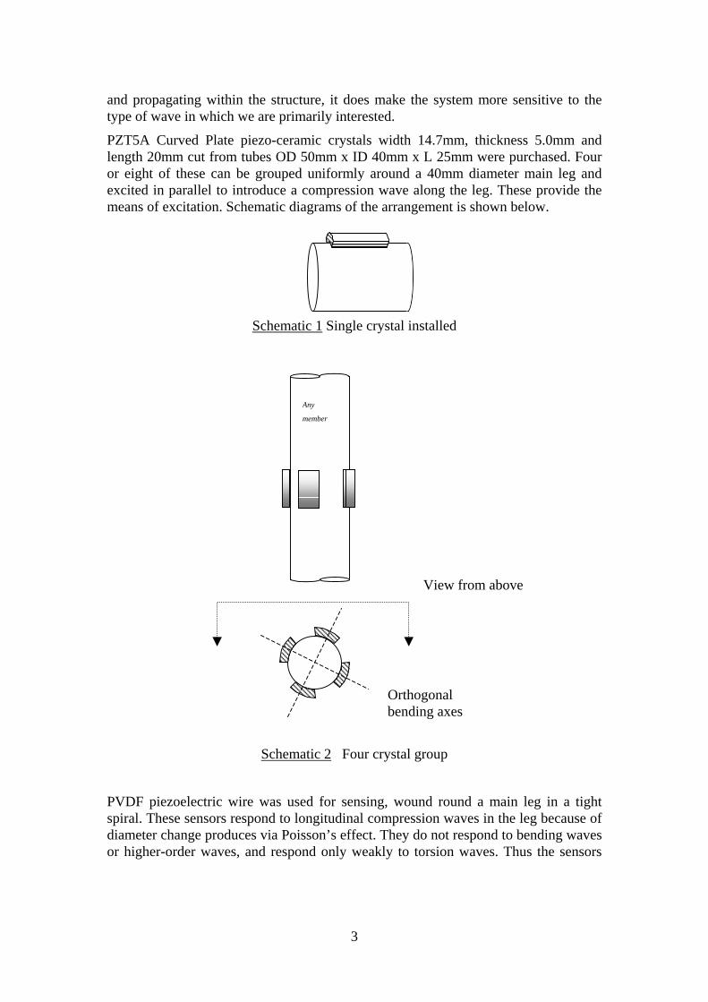
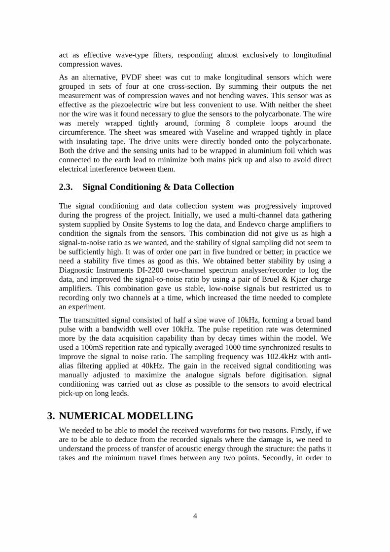
PZT5A Curved Plate piezo-ceramic crystals width 14.7mm, thickness 5.0mm and length 20mm cut from tubes OD 50mm x ID 40mm x L 25mm were purchased. Four or eight of these can be grouped uniformly around a 40mm diameter main leg and excited in parallel to introduce a compression wave along the leg. These provide the means of excitation. Schematic diagrams of the arrangement is shown below.

Schematic 1 Single crystal installed

Schematic 2 Four crystal group

PVDF piezoelectric wire was used for sensing, wound round a main leg in a tight spiral. These sensors respond to longitudinal compression waves in the leg because of diameter change produces via Poisson’s effect. They do not respond to bending waves or higher-order waves, and respond only weakly to torsion waves. Thus the sensors

View from above

Orthogonal bending axes

Any

member

3

act as effective wave-type filters, responding almost exclusively to longitudinal compression waves.

As an alternative, PVDF sheet was cut to make longitudinal sensors which were grouped in sets of four at one cross-section. By summing their outputs the net measurement was of compression waves and not bending waves. This sensor was as effective as the piezoelectric wire but less convenient to use. With neither the sheet nor the wire was it found necessary to glue the sensors to the polycarbonate. The wire was merely wrapped tightly around, forming 8 complete loops around the circumference. The sheet was smeared with Vaseline and wrapped tightly in place with insulating tape. The drive units were directly bonded onto the polycarbonate. Both the drive and the sensing units had to be wrapped in aluminium foil which was connected to the earth lead to minimize both mains pick up and also to avoid direct electrical interference between them.

2.3. Signal Conditioning & Data Collection

The signal conditioning and data collection system was progressively improved during the progress of the project. Initially, we used a multi-channel data gathering system supplied by Onsite Systems to log the data, and Endevco charge amplifiers to condition the signals from the sensors. This combination did not give us as high a signal-to-noise ratio as we wanted, and the stability of signal sampling did not seem to be sufficiently high. It was of order one part in five hundred or better; in practice we need a stability five times as good as this. We obtained better stability by using a Diagnostic Instruments DI-2200 two-channel spectrum analyser/recorder to log the data, and improved the signal-to-noise ratio by using a pair of Bruel & Kjaer charge amplifiers. This combination gave us stable, low-noise signals but restricted us to recording only two channels at a time, which increased the time needed to complete an experiment.

The transmitted signal consisted of half a sine wave of 10kHz, forming a broad band pulse with a bandwidth well over 10kHz. The pulse repetition rate was determined more by the data acquisition capability than by decay times within the model. We used a 100mS repetition rate and typically averaged 1000 time synchronized results to improve the signal to noise ratio. The sampling frequency was 102.4kHz with anti-alias filtering applied at 40kHz. The gain in the received signal conditioning was manually adjusted to maximize the analogue signals before digitisation. signal conditioning was carried out as close as possible to the sensors to avoid electrical pick-up on long leads.

3. NUMERICAL MODELLING We needed to be able to model the received waveforms for two reasons. Firstly, if we are to be able to deduce from the recorded signals where the damage is, we need to understand the process of transfer of acoustic energy through the structure: the paths it takes and the minimum travel times between any two points. Secondly, in order to

4

develop our damage location algorithms we needed noise-free data on which to test them.

Our numerical model is based on the same structure used for the physical scale model: the upper half of the Claymore jacket (see Plate 1). It assumes that the jacket consists essentially of beam-like members joined at nodes. It models waves travelling along members with one velocity only, and models the division of energy at a node as a simple equipartition among the joined members.

Thus our model ignores wave types other than longitudinal waves. There are several reasons for this simplified approach. Our damage location algorithms use only the earliest arrival of energy at a sensor from a point of damage, and this will almost always have travelled through the structure at the longitudinal-wave velocity. Other wave types (torsion waves, bending waves, Lamb waves) will travel at lower velocities and can be left out of the modelling. Our model aims to represent the timing of the compressional waves travelling through the structure correctly but not their magnitude.

To some extent we are making a virtue of a necessity, since the resources of the project would not be sufficient to allow the creation of a more detailed numerical model of the acoustics of the structure. Nor would it be possible to run such a model in a reasonable time on a desktop PC running MS Windows. However it is also true to say that a more detailed model would be of questionable value: it would be unlikely to represent the properties of the physical structure sufficiently accurately, and adjusting it to fit observations on the structure would be a complex and difficult task. The virtue of a single-wave-type model is that it is relatively easy to bring it into agreement with the physical model, as we shall see.

The modelling algorithm uses a modified time-stepping approach that propagates an acoustic impulse arriving at any node to its immediate neighbours (i.e. to nodes directly connected to it by members). An acoustic impulse is introduced at the transmitter location on the structure, at time step zero. Its energy is divided equally between the members connected to the transmitter location. The precise arrival time of the impulse at the node at the far end of each member is then calculated, and the amplitude of the impulse is entered into the time-record for that node at the time step nearest to the precise arrival time. The event is “tagged” with the difference between the time of the step and the precise arrival time. The size of the time step is kept smaller than the travel time along the shortest structural member.

The algorithm then proceeds to the next time step for which (given the known transit times along the various members) it is possible that an event may have arrived. If there are any events associated with any node of the structure, these are first examined to see if any of the events at any one node coincide precisely in time (i.e. if their time-difference tags are equal). If so, the events are amalgamated in such a way as to conserve acoustic energy. All events at each node are then propagated forward in time to its immediate neighbours, taking their time-difference tags into account. Again, they are propagated to the nearest time step, and tagged with the difference between the time of the step and the precise arrival time. This process is then repeated until the

5

required number of time steps has been covered. This is set to be at least equal to the maximum acoustic transit time across the structure, and usually longer.

This approach is better than simple time stepping because it enables transit times to be modelled accurately, avoiding numerical dispersion without having to use a very short time step, while still ensuring that all possible acoustic propagation paths are included in the model. This results in a computationally efficient algorithm that can model propagation between many transmitters and receivers through a highly complex structure in a few tens of minutes on a PC.

Note that in our current implementation of this model we have chosen to identify model “nodes” with physical nodes of the structure. We are free to include more nodes in the model if we wish: for example we could place several “nodes” along each member. This would increase the resolution with which the damage location algorithms (which derive their knowledge of the structure from the forward-modelling algorithms) could locate damage when the damage does not occur at a structural node.

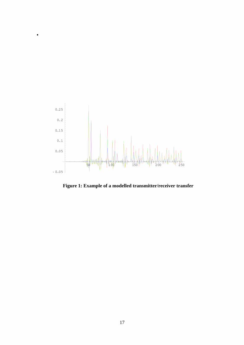
The numerical model leads to predicted transfer functions between each transmitter-receiver pair. The propagation algorithm yields a list of events with their times and amplitudes at each receiver, for each transmitter. These are converted to sampled time series data by using standard sinc-interpolation to add each event to the time series. An example appears in Figure 1 below. In this figure, the transfer function before damage is shown in red; that after damage is shown in green; and the difference between the two is shown in blue. It gives some indication of the complexity of the process of acoustic transmission: near the onset of the trace, individual events (representing reflections from nodes) can be distinguished. However these rapidly decline in amplitude while becoming more closely spaced in time, so that the difference trace soon becomes a seemingly random continuum.

Note that no bandwidth limitation has been applied to this trace, so that each event appears as a sinc-function, that is to say a positive-going pulse accompanied by low-level “ripples”. We have made no attempt to model absorption, which would cause the signal to decrease rapidly with time.

4. CALIBRATING THE NUMERICAL MODEL AGAINST THE PHYSICAL MODEL As in any situation where one is trying to match the behaviour of a real structure with a numerical model, the agreement between the two can be improved by comparing predictions with measurement. Figure 2 below shows a scatter plot of predicted first arrival times versus measurements for a set of six transmitters at the top of the structure and eight at the bottom.

Note that the numerical model times have been calculated using the measured longitudinal-wave velocity in the plastic. This plot suggests that there is an additional propagation delay that is larger the further the transmitter is from the receiver. Furthermore, this delay increases faster than linearly with travel time.

6

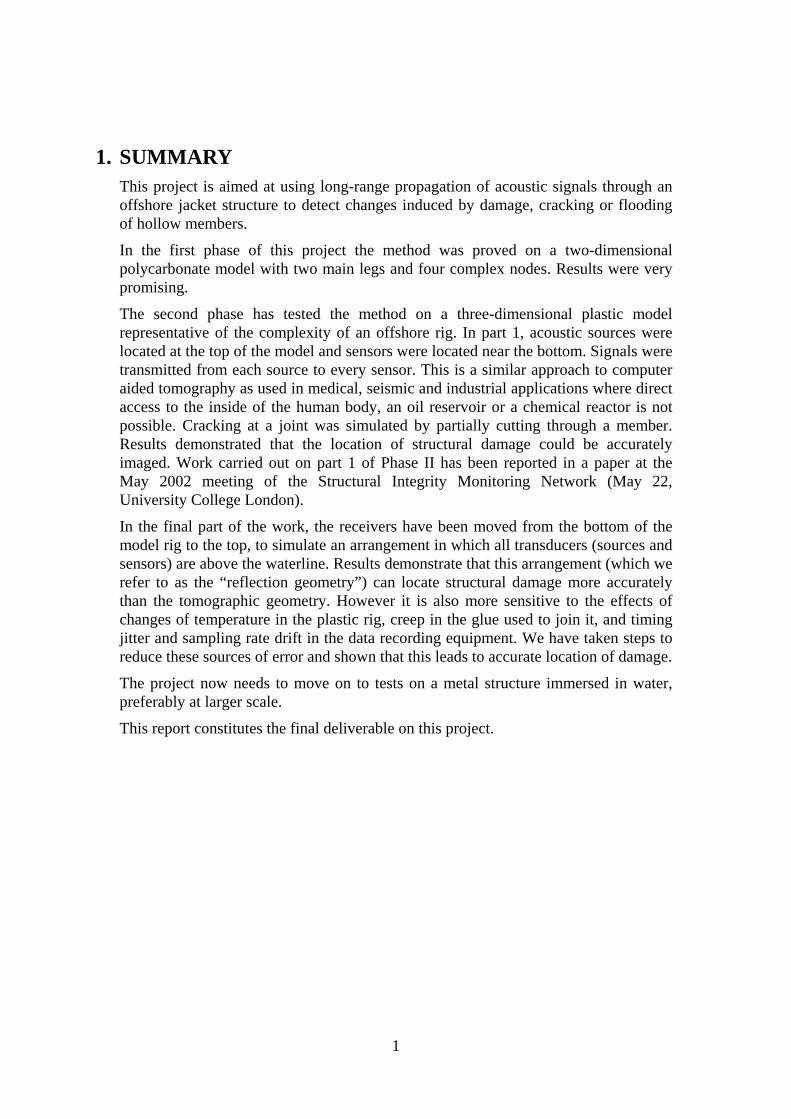
This delay is probably mainly due to delays in propagation through nodes, which are likely to have quite complicated dynamics which it is beyond the scope of this project to model. To get around this problem we simply applied a correction to the model travel times based using a best-fit quadratic expression calculated from the transmitter/receiver offsets in x, y and z directions. The errors in predicted arrival times after applying this correction appear in figure 3 below. The errors are significantly reduced.

5. SIGNAL CHARACTERISTICS Before moving on to describe our damage location algorithms, we shall give an example of the results from numerical and physical scale-model versions of an experiment in which one of the main legs of the structure was damaged. The layout of the transmitters and receivers was the “tomographic” arrangement: transmitters at top, receivers at bottom.

5.1. Numerical Model results

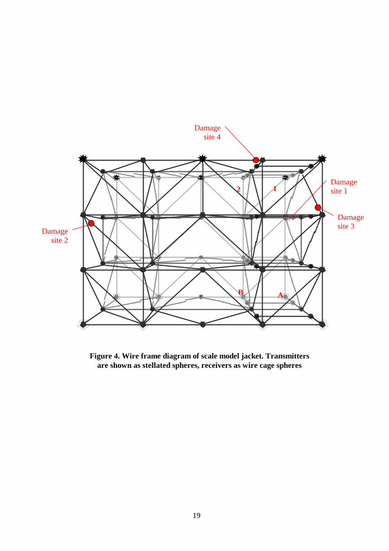
The experiments used six transmitters at the top of the structure and eight receivers at the bottom. Their positions are indicated in the wire-frame diagram of the structure shown in Figure 4 below. One of the main vertical legs was severed. The small red sphere shows the damage location. It is immediately below the node at the right-hand rear, one down from the top.

Figure 5 shows the modelled signal transmitted down the vertical leg on which the damage is located, from the transmitter at the top (shown by a red “1”) to the receiver at the bottom (red “A”). Note that the signal was only calculated up to 330 time steps. The difference (blue) signal shows the effect of the damage. It produces a large effect, which starts at the onset of the signal: because the damage lies on the direct transmission path from transmitter to receiver, the effect of the damage is evident in the first arrival. This is of great significance when inverting these data to locate the damage.

Figure 6 shows the signal that is obtained by transmitting from the node to the left (red “2” in Figure 1) to receiver “A”. The difference in signals still starts at the signal onset, because the damage lies on the shortest path from transmitter to receiver. However it is much smaller, because the shortest path is no longer unique. There are in fact five paths of equal length that are shorter than any others, and only one of these passes through the damage point. Hence most of the energy in the direct arrival is unaffected.

Figure 7 shows the signal that is obtained by transmitting from node “2” to receiver “B”. The damaged node no longer lies on the direct path, and consequently the difference caused by the damage occurs later than the first arrival. Whereas the first arrival is at time step 93, the difference first appears at step 144. The difference signal is small.

7

5.2. Physical Model Results

We ran into significant difficulties with signal stability, for three reasons. Firstly, the adhesive used to join the polycarbonate members did not set solid but remained in a visco-elastic phase when set. It is exceedingly difficult to glue polycarbonate. The best adhesive is actually a solvent and vapourizes in seconds. It was not possible to assemble the complex joins in the short time available with this solvent. Instead we used the only other glue recommended for this material – it is highly toxic and requires care in application. Unforunately it turned out to be highly temperature dependent in its properties, and we could only obtain consistent results by maintaining the rig at a constant temperature. We achieved this by wrapping individual members and nodes in insulating material, and containing the entire structure in an insulating “tent”. The room outside was then maintained at around 20°C using normal thermostatic heating controls, and this proved to be acceptable, although drift has always remained evident in the results. A further improvement was eventually achieved by holding the room at 20oC as before and in additional controlling the temperature inside the ‘tent’ at 26oC.

The second difficulty was that the sampling frequency of the recording system turned out not to be stable enough. It was of order one part in five hundred or better; in practice we need a stability five times as good as this. It would not be difficult to achieve this level of stability now that its importance is evident. Again, however, results are degraded.

Lastly the sampling was not synchronised with the transmission, which caused timing “jitter”. For future work a solution to this jitter would be to use the same digital clock to generate the transmitted pulse as is used to sample the received signal.

Figure 8 shows the measured signal transmitted down the vertical leg on which the damage is located, from the transmitter at the top (shown by a red “1”) to the receiver at the bottom (red “A”). The difference (blue) signal shows the effect of the damage. As in the numerical model results, the damage produces a large effect, starting at the onset of the signal.

Note that the visual appearance is very different from the modelled data: the data here are band limited and have as many negative-going as positive-going excursions. Absorption is also causing higher frequencies to be attenuated preferentially at later times.

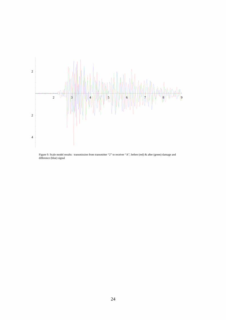
Figure 9 shows the signal obtained by transmitting from transmitter “2” to receiver “A”. The difference in signals still starts at the signal onset, because the damage lies on the shortest path from transmitter to receiver. As in the numerically modelled results, it is smaller. It is interesting to note that it is not as small: evidently the route via the damage point is preferred to others (i.e. carries relatively more energy) in the scale model (not surprising since its cross section is larger).

Finally, figure 10 shows the signal from transmitter “2” to receiver “B”. The onset of the difference is later than the onset of the trace, and the difference signal is smaller in relation to the pre-damage signal.

8

6. DAMAGE LOCATION ALGORITHMS We have developed two different algorithms. Both depend on the arrival times of “difference events” being identified on the recorded traces. This requires arrival times of major differences to be picked out of the recorded time signals. So far we have carried out this process manually. We have looked at automated means of picking, some of which appear promising, but further development will be required before they are sufficiently reliable.

The first of our two algorithms accepts not only the earliest-arriving difference events but also subsequent events as well. For each identified event on each trace, it calculates all possible paths by which the signal can have travelled from transmitter to receiver. All nodes that lie on each of these possible paths are possible damage sites, and the algorithm collects the possible sites associated with each event on each trace into a set. The algorithm calculates a similar set of such possible damage sites for each signal and each event; it then takes the intersection of these sets (i.e. chooses the node or nodes which belong to all of them) as its final indication of possible damage site(s).

We have tested this algorithm on model data and obtained good results. However its computation times can be extremely long (later events can be associated with millions of possible paths). The ability to handle multiple events on one signal has turned out not to be an advantage in practice, since on real data it becomes hard to distinguish genuine events from background noise after the arrival of the first event.

For these reasons we have concentrated our efforts on a simpler and more robust algorithm. This algorithm works only with the earliest-arriving damage event on each trace. This is in line with the philosophy underlying our approach to modelling, which is to calculate shortest-path travel times using longitudinal wave speeds (i.e. it is likely to get earliest arrival times right but likely to estimate later arrival times less accurately).

This algorithm works by considering each node of the model in turn to be a possible damage site. It works out the expected earliest damage event arrival time for each transmitter/receiver combination and compares this with the arrival time of the first difference event picked on the recorded data. The time difference is squared and taken as a measure of error in the assumption that the selected node is the site of the damage. The squared error is summed over all transmitter/receiver pairs and divided by the number of contributing pairs to produce a mean-squared timing error for that node.

The exercise is repeated for each node of the structure. The result is a “map” of mean-squared error over the structure. The node at which the mean-squared error is least is considered to be the damaged node. The confidence of identification can be measured by the relative size of the error at that node compared to others. We shall refer to this as the “least mean-square” (LMS) imaging method.

One elaboration of this method that occasionally improves the imaging of noisy data is to preferentially weight the results in favour of transmitter/receiver signals for which the difference event arrives soon after the first arrival. Thus later events, whose

9

timing is usually more difficult to pick accurately, are given less weight in the imaging process. This is achieved by weighting the square error for a given signal by the factor

( )nd

0

11

1

τττ −+

in which:

1τ is the first arrival time;

dτ is the arrival time of the damage event;

0τ is a scale time such that damage events occurring later τ0 after τ1 are weighted less heavily;

n is the weighting exponent: later events are weighted less strongly if n is higher.

Common values used for imaging our scale model data are n=4 and sec10 m=τ .

7. MAGNITUDE OF DIFFERENCE SIGNALS AND DETECTABILITY OF DAMAGE The advantage of using low frequency waves to monitor structural integrity is that they can travel a long way, and so fewer transmitters and receivers are required. The disadvantage is that a crack in a structural member must be well developed before it will introduce significant reflections of the waves. A test was carried out using the simple polycarbonate model of a joint shown in Figure 11. Table 1 below shows a measurement of the change in amplitude of the wave transmitted past the joint when the outgoing member is partially cut through. It is evident that, in order to get a difference signal whose amplitude is big enough to be readily detectable, the member has to be cut most of the way through. Low frequency waves are not suitable for the detection of small cracks. This effect was confirmed on the model jacket. A cut at 10mm from a diagonal strut showed no perceptible difference in signal after 25% of the area was cut. After 50% area was cut there was a very small difference signal and after 75% was cut there were major differences.

However, offshore jacket structural members will flood once a crack penetrates the wall. The effect of the water inside the member is then likely to be larger than the crack, introducing a change in reflection coefficient of order 20-30%. We expect that in practice it will be flooded members rather than cracks that will be detected.

10

Table 1. effect of a cut on the signal transmitted through the joint shown in Figure 11.

Cut area as percentage of total Difference signal rms / original signal rms

1 0.02%

10 0.24%

20 0.6%

25 0.8%

30 1.02%

40 1.58%

50 2.39%

75 7.33%

90 22.33%

8. TOMOGRAPHIC GEOMETRY EXPERIMENTS We will show here the results of two tomographic-geometry experiments. In each, a set of measurements between sources at the top of the structure and sensors at the bottom was carried out before and after damage was artificially induced by cutting most of the way through a structural member.

8.1. Damage on a Vertical Leg

In Section 4 we presented and discussed example signals obtained before and after damage to a main leg. The point of damage is shown in Figure 4 as “damage site 1”.

We applied the LMS damage location algorithm both to the data derived from the numerical model and to the data recorded on the physical model.

The results of applying the LMS imaging method to the numerical model data are shown in Figure 12 below. Errors at each node are coded via both the colour and the size of a sphere centred at that node. The actual damage site was the first node below the top of the rightmost vertical. The error is indeed smallest at this node, where it is zero (since the numerically modelled data is error-free), but it is also very small on the nodes above and below as the figure shows. The vertical position discrimination is not very strong, and a small amount of error in the data could result in the wrong node being identified.

The error is largest on the far side of the rig from the damage site.

11

If we now apply the same imaging method to real data recorded in the same way, we obtain the error distribution shown in Figure 13. The damage is correctly located, but again the vertical discrimination is not very strong.

8.2. Damage on a Diagonal Strut

The exercise was repeated, this time for damage on a diagonal strut at the point labelled “damage point 2” in Figure 4. As in section 8.1, we produced maps of LMS error using both data produced with the numerical model and data measured on the physical model.

Results for the simulated data are shown in Figure 14. As one might expect, the damage is in fact correctly located. However, once again, vertical discrimination is poor and the LMS error is small for points above and below the damage location.

Figure 15 shows the results obtained from the physical model data. In this case, the estimated position of the damage is at the bottom end of the diagonal strut instead of the top. This appears to us to be an inherent weakness of the tomographic geometry: it shows limited vertical discrimination and is liable to mis-locate damage vertically as a result, but not by more than one strut length.

Numerical simulations of reflection geometry, with sources and receivers all at the top of the rig, indicated that the vertical resolution should be much improved. It would be a distinct advantage if the equipment could all be kept above the waterline. Consequently the next set of experiments were with the reflection geometry.

9. REFLECTION GEOMETRY EXPERIMENTS Two experiments have been carried out, one before the improvements to the rig temperature stability and data gathering system and one after. Both were carried out on the polycarbonate rig shown in Plate 1. The positions of sources and receivers are indicated in the wire-frame diagram in Figure 1, in which the sources are shown as stellated spheres and the receivers as wire-cage spheres, all located at the top of the structure (in practice the transducers were attached to the vertical legs immediately above the nodes).

9.1. Pre-Improvement Experiment

The damage in this case was the complete severing of a member at the point indicated by the red disc marked “damage site 3” in Figure 4.

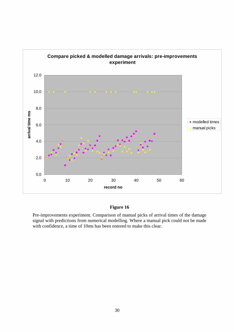
The data produced by this experiment were of poor quality because of the drift discussed earlier (not because of random noise). Figure 16, which compares predicted and manually picked damage event arrival times, indicates the poor quality of the data. The scatter between the two is greater, with a strong tendency for events arriving later than about 4ms to be picked too early. These are records for which the damage

12

point is a long way off the direct path between source and sensor. The higher levels of spurious signal on this data set mask later arrivals, which are usually weaker.

Figure 17 shows the error-sphere diagram for this experiment, with the true and estimated damage locations shown: the algorithm has mis-located the damage by one node spacing to the rear and one to the left. The early picks on records from sources and sensors far from the damage point have pulled the estimated damage position away from the true location towards the centre of the rig.

9.2. Post-Improvement Experiment

The structure was “damaged” by cutting most of the way through a horizontal strut at the position marked by a red disc labelled “damage site 4” in Figure 4.

The data set is of good quality. Consequently it was usually possible to pick the arrival times of the difference events caused by the damage. However, as we have found on previous data sets, there are a few source/sensor combinations for which the damage makes so little difference to the signal that an arrival time cannot be picked with any confidence. We have also found that when the source and sensor are coincident the damage signal is drowned out by the direct signal from the source. The signal from reverberation in the structure close to the source/sensor location is so much stronger than the signal scattered from the damage that the damage signal is lost in the drift of the reverberation signal, even when that drift is very small.

The results are shown in Figure 18 as a graphical comparison of manual picks of damage arrival times with the predictions of numerical modelling. On records where a manual pick could not be made with confidence, a very late pick time of 10ms has been entered to make this clear. Seventeen out of forty-eight records could not be picked; of these, six were coincident source/receivers. For the remaining thirty-one records, the error is below ½ millisecond. The records are shown in the order they were recorded.

These results were input to the LMS damage location algorithm. The resulting error-sphere map is shown in Figure 19. The damage is correctly located to the nearest node. It is worthy of note that the data were of such good quality that the noise-control parameters (n and τ0) were not needed: the damage was correctly located regardless of what values they were given, or of whether they were used.

10. EFFECT OF TOPSIDES A potential difficulty in applying this method to an offshore platform is that topsides changes (such as moving massive equipment from one place to another) could cause changes to signals, because the topsides platform is rigidly mounted on the jacket. The following section describes a method of isolating the topsides from the jacket structure acoustically so that this does not occur.

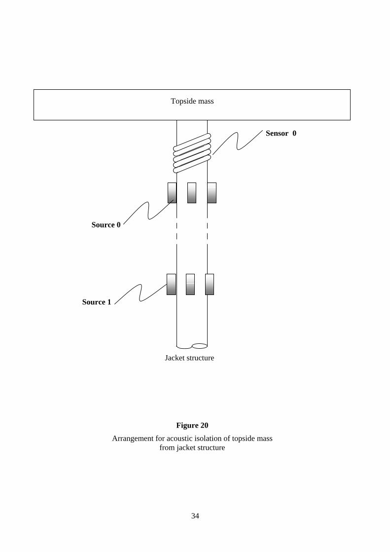
Consider a leg of the structure on which the topsides rests. Figure 10 is a schematic diagram showing a sensor (a coil of piezo-wire, “sensor 0”) and a four-segment source (“source 0”) mounted immediately beneath the topside platform. Some way

13

below this is a second source (“source 1”). Source 1 can be considered as the primary source whose signals we want to sense at various points on the structure; source 0 is a secondary source which is used purely to prevent any signal from reaching the topside sensor. This is achieved as follows.

Suppose )(1 ωiH and )(0 ωiH represent the frequency domain responses at a general point i on the structure to applied unit impulses at sources 1 and 0 respectively. Then

a force )()(

00

01

ωω

HH

applied at source 0 will produce a response at point 0 that equals the

response at this location due to a unit force at source 1. Thus if source 0 is driven with

a force )()(

00

01

ωω

HH

− at the same time that a unit impulse is applied at source 1, there

will be zero signal at sensor 0: no signal will reach the topside, and no topside signal will return to the sensors.

This procedure will of course modify the signals received at the points i elsewhere on the structure. Instead of the signal )(1 ωiH , sensor i will now see a signal given by

)()(

)()(00

01010 ω

ωωω

HH

HHH iici −= .

This signal will be very small if sources 0 and 1 are too close together: the two sources will “fight” each other. There therefore needs to be some vertical separation between the two sources. This need not be large; in fact the main restriction on it is that it should not be equal to half a wavelength at the highest frequency of interest (otherwise it will partly cancel the signal from the primary source at this frequency).

Signalsneed not be applied to sources 0 and 1 simultaneously. Since the principle of superposition applies to acoustic signals (certainly at the modest levels of signals used in these experiments), the two can be driven at different times. The processing can be applied subsequently to combine the responses and calculate the desired result.

We had hoped to test this procedure on our rig. However, owing to the amount of time and effort required to overcome problems of signal drift, we have been unable to do so. This procedure is tried and tested in other contexts, principally active control of noise in ducts, and there is no serious doubt that the principle works.

14

11. CONCLUSIONS We have presented results for two types of measurement geometry: tomographic, with sources at the top of the structure and sensors at the bottom, and reflection, with the sensors moved to the top. Both approaches can be used successfully to locate damage. The method is effective using very small numbers of source and sensor positions in proportion to the number of structural members being monitored for damage.

The tomographic geometry shows limited vertical resolution. This is because the ray paths are mostly close to the vertical, which makes it difficult for an algorithm based on transmission time via the damage point to determine how far down the structure the damage location lies. The reflection geometry does not suffer from this drawback, because the time of arrival of damage events is very sensitive to the vertical position of the damage.

The reflection geometry is also much more practical from the point of view of application to offshore structures, because all transducers and wiring can be located above the splash zone.

Our work has shown that signal stability is very important: the signals must not change unpredictably unless the structure suffers damage. A major difficulty with our experiments has been that signals have drifted over time. Most of the sources of drift in our experiment would not occur, or could easily be eliminated, in use on a real jacket. The effects of temperature drift would not be as severe; structural creep would be most unlikely; and instrumental drift could easily be eliminated. However other sources of drift are possible: for example the effect of tidal changes of water level, and parametric effects of wave-induced lateral forces on the structure. Tidal changes would obviously be diurnal, and it should be possible to identify and disregard them or time the measurements to avoid the variation. If waves showed any effects, then in principle it should be possible to remove them in the same way as the waves will also be periodic.

Another source of unwanted change in the signals might be changes in mass distribution topsides (i.e. on the platform itself, above the transducers). We have devised a way of preventing this. Our limited resources have not allowed us to test this active control procedure on our experimental set up but we are confident that it will work.

15

12. THE NEXT STAGE The method has been adequately tested in the laboratory. It now needs to be tested on a steel structure immersed in water, preferably at a larger scale. The data gathering system needs to be sufficiently stable to avoid introducing errors when looking for small changes in signals. Points that need to be addressed include:

• Designing sources and sensors suitable for a steel structure and robust enough to be left in place for years;

• Confirming that unpredictable signal drift in a steel structure is small enough to allow the method to work effectively (drift less than 5% of peak signal magnitude);

• Assessing the extent of periodic signal drift due to the actions of tide and of wave motion, and predicting and eliminating them;

• Assessing the influence of background noise;

• Assessing the influence of changes in mass on the topsides and testing out procedures for dealing with this.

16

•

50 100 150 200 250

- 0.05

0.05

0.1

0.15

0.2

0.25

Figure 1: Example of a modelled transmitter/receiver transfer

17

Error in arrival time vs modelled arrival time

-3.00

-2.50

-2.00

-1.50

-1.00

-0.50

0.00

0.50

1.00

1.50

2.00

2.50

3.00

0 0.5 1 1.5 2 2.5 3 3.5

Modelled arrival time ms

ms observed-modelled ms

Figure 2. Predicted vs. observed travel times

Error in arrival time vs corrected modelled arrival time

-3.00

-2.50

-2.00

-1.50

-1.00

-0.50

0.00

0.50

1.00

1.50

2.00

2.50

3.00

0 0.5 1 1.5 2 2.5 3 3.5

Modelled arrival time ms

Cor

rect

ed e

rror

ms

observed-corrected modelled ms

Figure 3: Errors after correcting model predictions

18

12

Figure 4. Wire frame diagram of scale model jacket. Transmitters are shown as stellated spheres, receivers as wire cage spheres

A B

12Damage site 1

Damage site 4

Damage site 3 Damage

site 2

19

Figure 6. Numerically-modelled time signal of transmission from transmitter “2” to receiver “A”, before (red) & after (green) damage and difference (blue) signal

100 200 300 400

0.02

0.04

0.06

0.08

0.1

Figure 5

Numerically-modelled signal transmitted down damaged leg from transmitter 1 to receiver A in Figure 4. The damage makes a large difference at the onset of thesignal.

Red: before damage

Green: after damage

Blue: difference

20

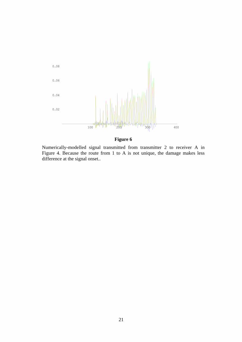
Figure 5. Numerically-modelled time signal of transmission down damaged leg, before (red) & after (green) damage and difference (blue) signal

100 200 300 400

0.02

0.04

0.06

0.08

Figure 6

Numerically-modelled signal transmitted from transmitter 2 to receiver A in Figure 4. Because the route from 1 to A is not unique, the damage makes lessdifference at the signal onset..

21

100 200 300 400

0.025

0.05

0.075

0.1

0.125

0.15

Figure 7. Numerically-modelled time signal of transmission from transmitter “2” to receiver “B”, before (red) & after (green) damage and difference (blue) signal Figure 7

Numerically-modelled signal transmitted from transmitter 2 to receiver B in Figure 4. The differences are small and occur some time after the signal onset because the damage does not lie on the direct signal route from 2 to B..

22

2 3 4 5 6 7 8 9

- 4

- 2

2

4

Figure 8. Scale model results: transmission from transmitter “1” to receiver “A”, before (red) & after (green) damage and difference (blue) signal

23

24

2 3 4 5 6 7 8 9

4

2

2

Figure 9. Scale model results: transmission from transmitter “2” to receiver “A”, before (red) & after (green) damage and difference (blue) signal

2 3 4 5 6 7 8 9

4

2

2

Figure 10. Scale model results: transmission from transmitter “2” to receiver “B”, before (red) & after (green) damage adifference (blue) signal

nd

12mm rod 3m long 16mm joint midway 40mm long cut

Figure 11

Polycarbonate model of a structural joint used to assess the effect of apartial cut on the signal transmitted past the joint

25

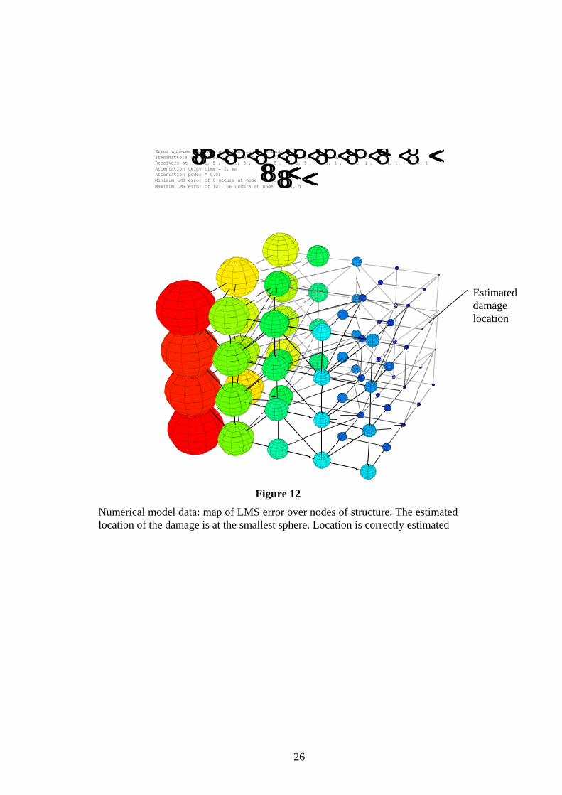
Error spheres for each node position on structureTransmitters at 881, 1, 5<, 81, 3, 5<, 81, 5, 5<, 81, 1, 1<, 81, 3, 1<, 81, 5, 1<<Receivers at 884, 1, 5<, 84, 2, 5<, 84, 4, 5<, 84, 5, 5<, 84, 1, 1<, 84, 2, 1<, 84, 4, 1<, 84, 5, 1<<Attenuation delay time = 2. msAttenuation power = 0.01Minimum LMS error of 0 occurs at node 882, 5, 1<<Maximum LMS error of 107.106 occurs at node 884, 1, 5<<

Estimated damage location

Figure 11. Numerically modelled data

Map of LMS error over nodes of structure. Damage site was first node below the top of the rear rightmost vertical.

Figure 12

Numerical model data: map of LMS error over nodes of structure. The estimatedlocation of the damage is at the smallest sphere. Location is correctly estimated

26

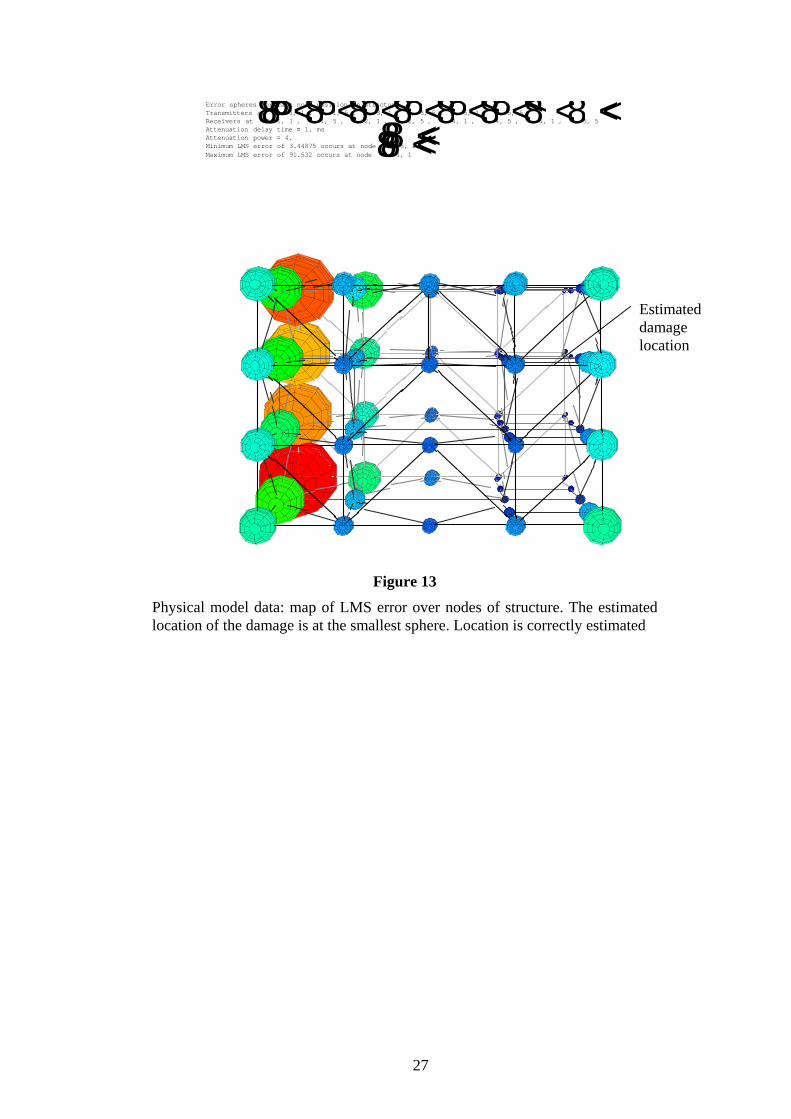
Error spheres for each node position on structureTransmitters at 881, 1, 1<, 81, 1, 5<, 81, 3, 1<, 81, 3, 5<, 81, 5, 1<, 81, 5, 5<<Receivers at 884, 1, 1<, 84, 1, 5<, 84, 2, 1<, 84, 2, 5<, 84, 4, 1<, 84, 4, 5<, 84, 5, 1<, 84, 5, 5<<Attenuation delay time = 1. msAttenuation power = 4.Minimum LMS error of 3.44875 occurs at node 881, 5, 1<<Maximum LMS error of 91.532 occurs at node 884, 1, 1<<

Figure 12. Scale model data

M

Estimated damage location

ap of LMS error over nodes of structure. Damage site was first node below the top of the rear rightmost vertical.

Figure 13

Physical model data: map of LMS error over nodes of structure. The estimatedlocation of the damage is at the smallest sphere. Location is correctly estimated

27

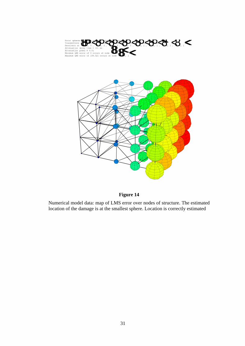
Error spheres for each node position on structureTransmitters at 881, 1, 5<, 81, 3, 5<, 81, 5, 5<, 81, 1, 1<, 81, 3, 1<, 81, 5, 1<<Receivers at 884, 1, 5<, 84, 2, 5<, 84, 4, 5<, 84, 5, 5<, 84, 1, 1<, 84, 2, 1<, 84, 4, 1<, 84, 5, 1<<Attenuation delay time = 10. msAttenuation power = 0.01Minimum LMS error of 0 occurs at node 882, 1, 5<<Maximum LMS error of 108.321 occurs at node 884, 5, 1<<

Figure 14

Numerical model data: map of LMS error over nodes of structure. The estimatedlocation of the damage is at the smallest sphere. Location is correctly estimated

31

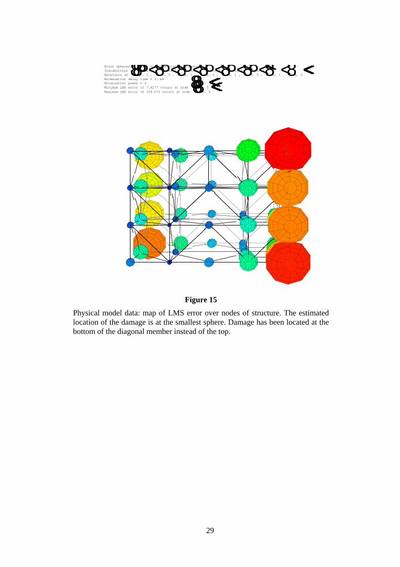
Error spheres for each node position on structureTransmitters at 881, 1, 1<, 81, 1, 5<, 81, 3, 1<, 81, 3, 5<, 81, 5, 1<, 81, 5, 5<<Receivers at 884, 1, 1<, 84, 1, 5<, 84, 2, 1<, 84, 2, 5<, 84, 4, 1<, 84, 4, 5<, 84, 5, 1<, 84, 5, 5<<Attenuation delay time = 1. msAttenuation power = 4Minimum LMS error of 7.4277 occurs at node 883, 2, 5<<Maximum LMS error of 104.073 occurs at node 881, 5, 5<<

F

Physical model data: map of LMS location of the damage is at the smabottom of the diagonal member inste

igure 15

error over nodes of structure. The estimatedllest sphere. Damage has been located at thead of the top.

29

Compare picked & modelled damage arrivals: pre-improvements experiment

0.0

2.0

4.0

6.0

8.0

10.0

12.0

0 10 20 30 40 50 60

record no

arriv

al ti

me

ms

modelled timesmanual picks

Figure 16

Pre-improvements experiment. Comparison of manual picks of arrival times of the damagesignal with predictions from numerical modelling. Where a manual pick could not be madewith confidence, a time of 10ms has been entered to make this clear.

30

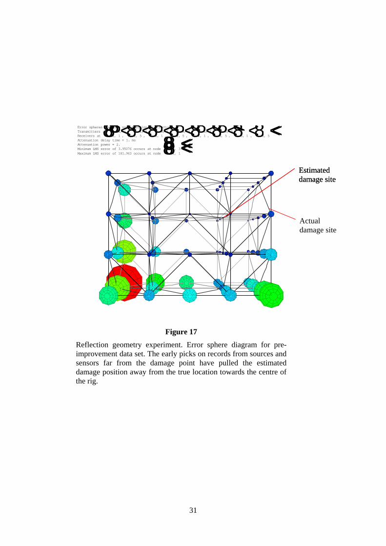
Error spheres for each node position on structureTransmitters at 881, 1, 1<, 81, 1, 5<, 81, 3, 1<, 81, 3, 5<, 81, 5, 1<, 81, 5, 5<<Receivers at 881, 1, 1<, 81, 1, 5<, 81, 3, 1<, 81, 3, 5<, 81, 4, 1<, 81, 4, 5<, 81, 5, 1<, 81, 5, 5<<Attenuation delay time = 1. msAttenuation power = 2.Minimum LMS error of 3.95076 occurs at node 882, 4, 3<<Maximum LMS error of 181.963 occurs at node 884, 1, 1<<

Actual damage site

Estimated damage site Estimated damage site

Figure 17

Reflection geometry experiment. Error sphere diagram for pre-improvement data set. The early picks on records from sources andsensors far from the damage point have pulled the estimateddamage position away from the true location towards the centre ofthe rig.

31

Compare picked & modelled damage arrivals: post-improvements experiment

0.0

2.0

4.0

6.0

8.0

10.0

12.0

0 10 20 30 40 50 60

record no

arri

val t

ime

ms

Manual picksModelled times

Figure 18

Post-improvements experiment. Comparison of manual picks of arrival times of thedamage signal with predictions from numerical modelling. Where a manual pick could notbe made with confidence, a time of 10ms has been entered to make this clear.

32

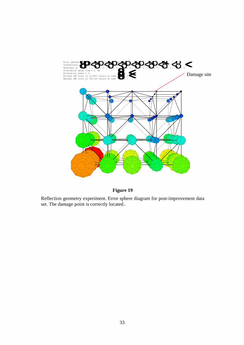
Error spheres for each node position on structureTransmitters at 881, 1, 1<, 81, 1, 5<, 81, 3, 1<, 81, 3, 5<, 81, 5, 1<, 81, 5, 5<<Receivers at 881, 1, 1<, 81, 1, 5<, 81, 3, 1<, 81, 3, 5<, 81, 4, 1<, 81, 4, 5<, 81, 5, 1<, 81, 5, 5<<Attenuation delay time = 1. msAttenuation power = 2.Minimum LMS error of 14.0827 occurs at node 881, 4, 5<<Maximum LMS error of 448.631 occurs at node 884, 1, 1<< Damage site

Figure 19

Reflection geometry experiment. Error sphere diagram for post-improvement data set. The damage point is correctly located..

33

Topside mass

Source 1

Sensor 0

Source 0

Jacket structure

Figure 20

Arrangement for acoustic isolation of topside mass from jacket structure

34

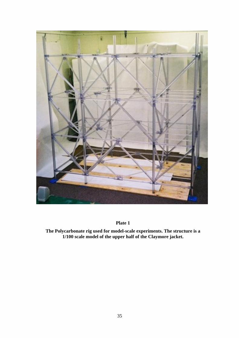
Plate 1

The Polycarbonate rig used for model-scale experiments. The structure is a 1/100 scale model of the upper half of the Claymore jacket.

35

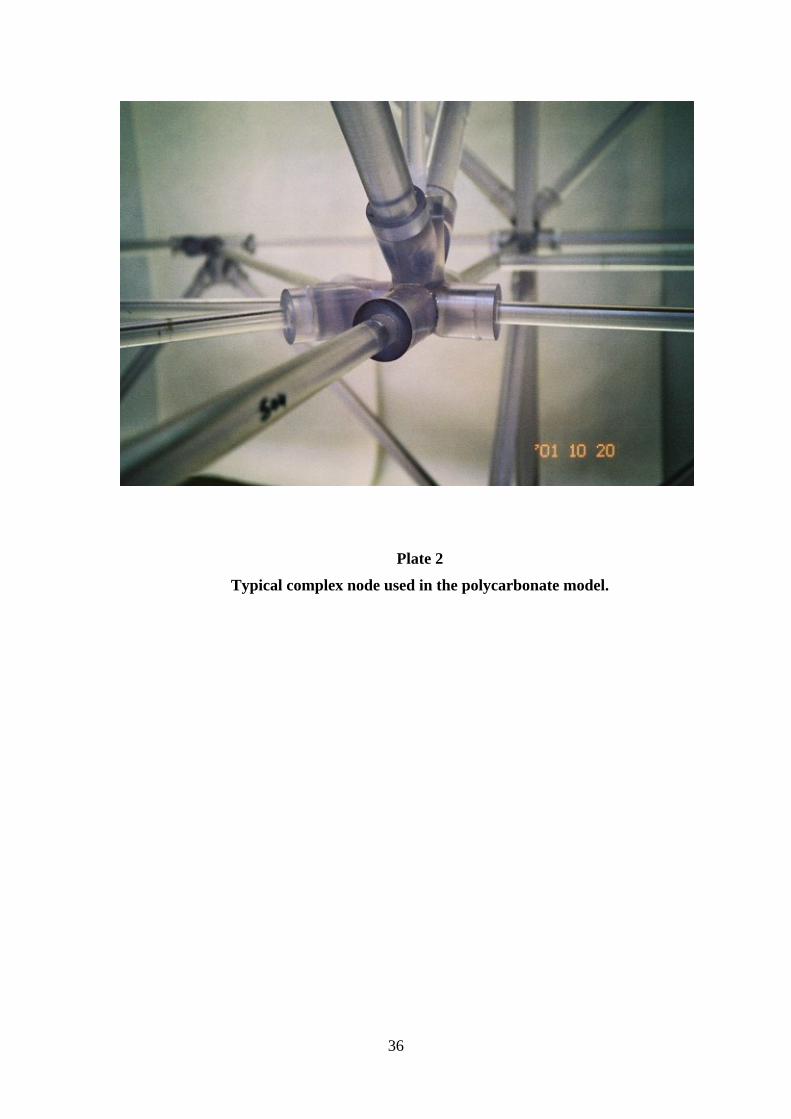
Plate 2

Typical complex node used in the polycarbonate model.

36

Printed and published by the Health and Safety ExecutiveC30 1/98

Printed and published by the Health and Safety ExecutiveC0.06 03/05

RR 326

£20.00 9 78071 7 62985 5

ISBN 0-7176-2985-6

Cost e

ffective

structu

ral m

onito

ring - A

n a

coustic m

eth

od

, phase

IIbH

SE B

OO

KS