Routing in Sensor NetworksRouting in Sensor Networks

Routing in Sensor NetworksRouting in Sensor Networks

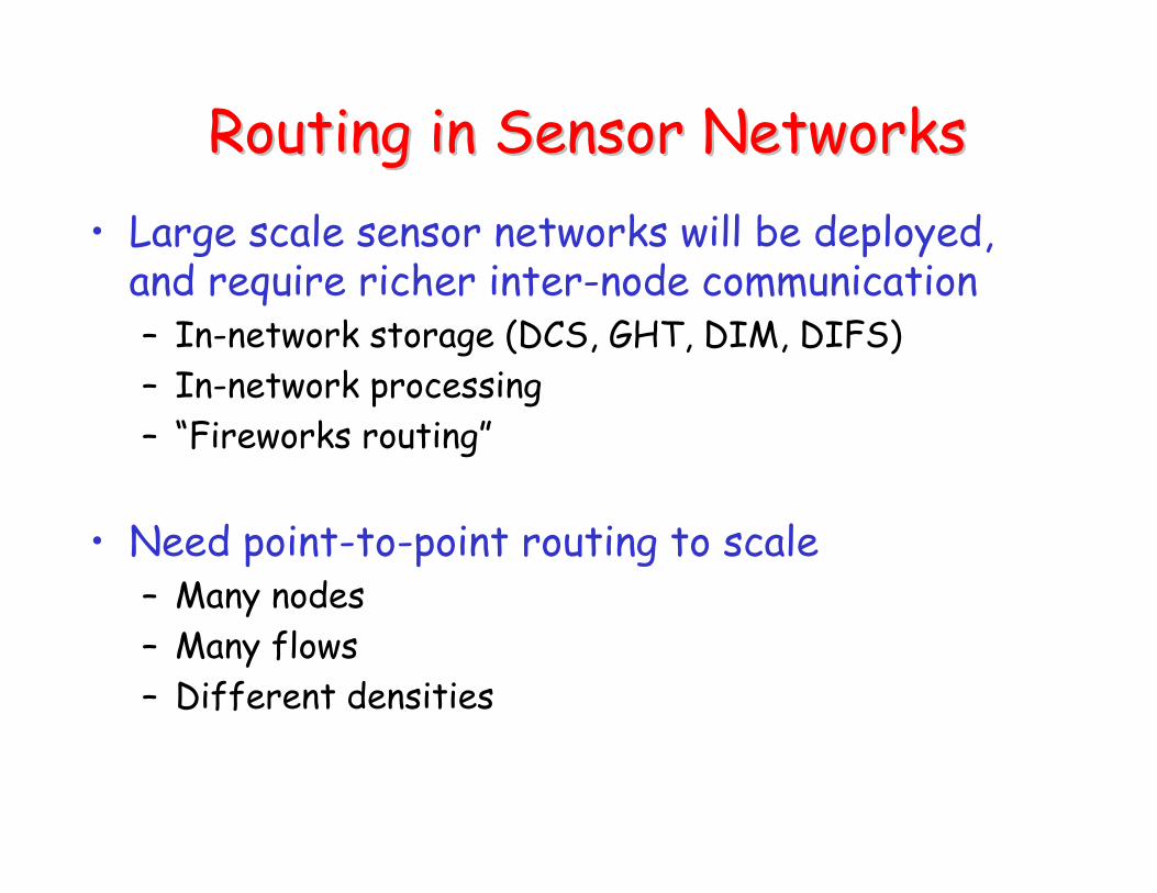
• Large scale sensor networks will be deployed, and require richer inter-node communication– In-network storage (DCS, GHT, DIM, DIFS)

– In-network processing

– “Fireworks routing”

• Need point-to-point routing to scale– Many nodes

– Many flows

– Different densities

Design GoalsDesign Goals

1. Simple – minimum required state, assumptions

2. Scalable – low control overhead, small routing tables

3. Robust – node failure, wireless vagaries

4. Efficient – low routing stretch

GPSR: Greedy Perimeter Stateless Routing GPSR: Greedy Perimeter Stateless Routing for Wireless Networksfor Wireless Networks

Brad Karp, H.T.Kung

Harvard University

GPSR: MotivationGPSR: Motivation

• Ad-hoc routing algorithms (DSR, AODV)– Suffer from out of date state

– Hard to scale

• Use geographic information for routing– Assume every node knows position (x,y)

– Keep a lot less state in the network

– Require fewer update messages

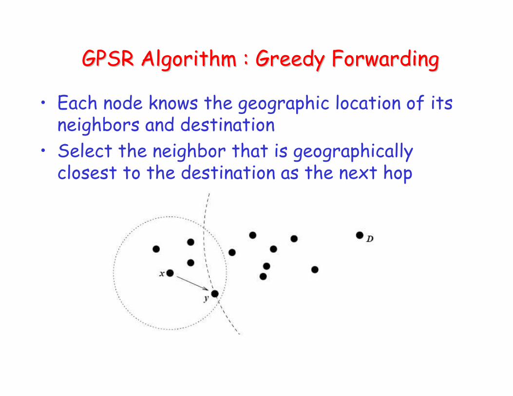
GPSR Algorithm : Greedy ForwardingGPSR Algorithm : Greedy Forwarding

• Each node knows the geographic location of its neighbors and destination

• Select the neighbor that is geographically closest to the destination as the next hop

GPSR Algorithm : Greedy Forwarding GPSR Algorithm : Greedy Forwarding (Cont.)(Cont.)

• Each node only needs to keep state for its neighbors

• Beaconing mechanism– Provides all nodes with neighbors’ positions.

– Beacon contains broadcast MAC and position.

– To minimize costs: piggybacking

GPSR Algorithm : Greedy Forwarding GPSR Algorithm : Greedy Forwarding (Cont.)(Cont.)

• Greedy forwarding does not always work!

Getting Around Void

• The right hand rule– When arriving at node x from node y, the next edge

traversed is the next one sequentially counterclockwise about x from edge (x,y)

– Traverse the exterior region in counter-clockwise edge order

Planarized Graphs

• A graph in which no two edges cross is known as planar.– Relative Neighborhood Graph (RNG)

– Gabriel Graph (GG)

Relative Neighborhood Graph

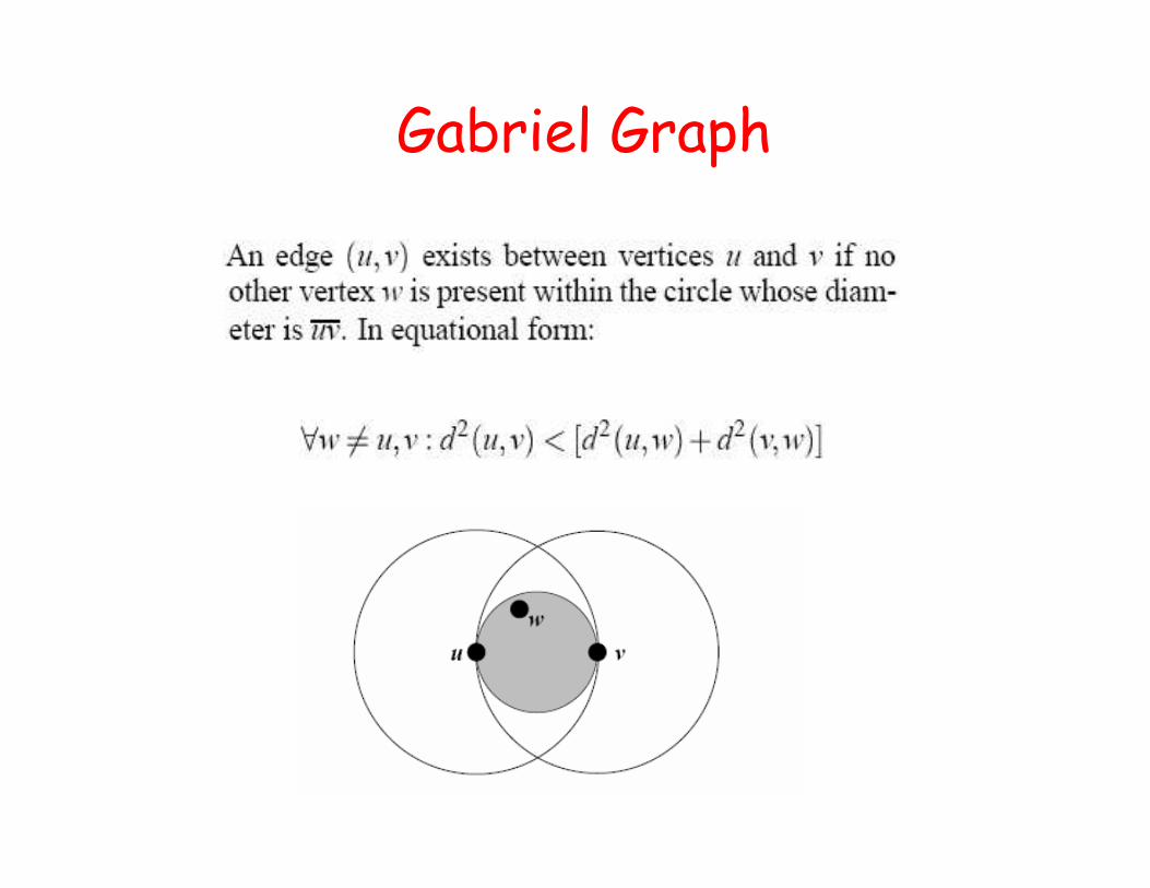
Gabriel Graph

Final Algorithm

• Combine greedy forwarding + perimeter routing– Use greedy forwarding whenever possible

– Resort to perimeter routing when greedy forwarding fails and record current location Lc

– Resume greedy forwarding when we are closer to destination than Lc

Protocol ImplementationProtocol Implementation

• Support for MAC-layer feedback

• Interface queue traversal

• Promiscuous use of the network interface

• Planarization of the graph

Simulation and EvaluationSimulation and Evaluation

• 50, 112, and 200 nodes with 802.11 WaveLAN radios.

• Maximum velocity of 20 m/s

• 30 CBR traffic flows, originated by 22 sending nodes

• Each CBR flows at 2Kbps, and uses 64-byte packets

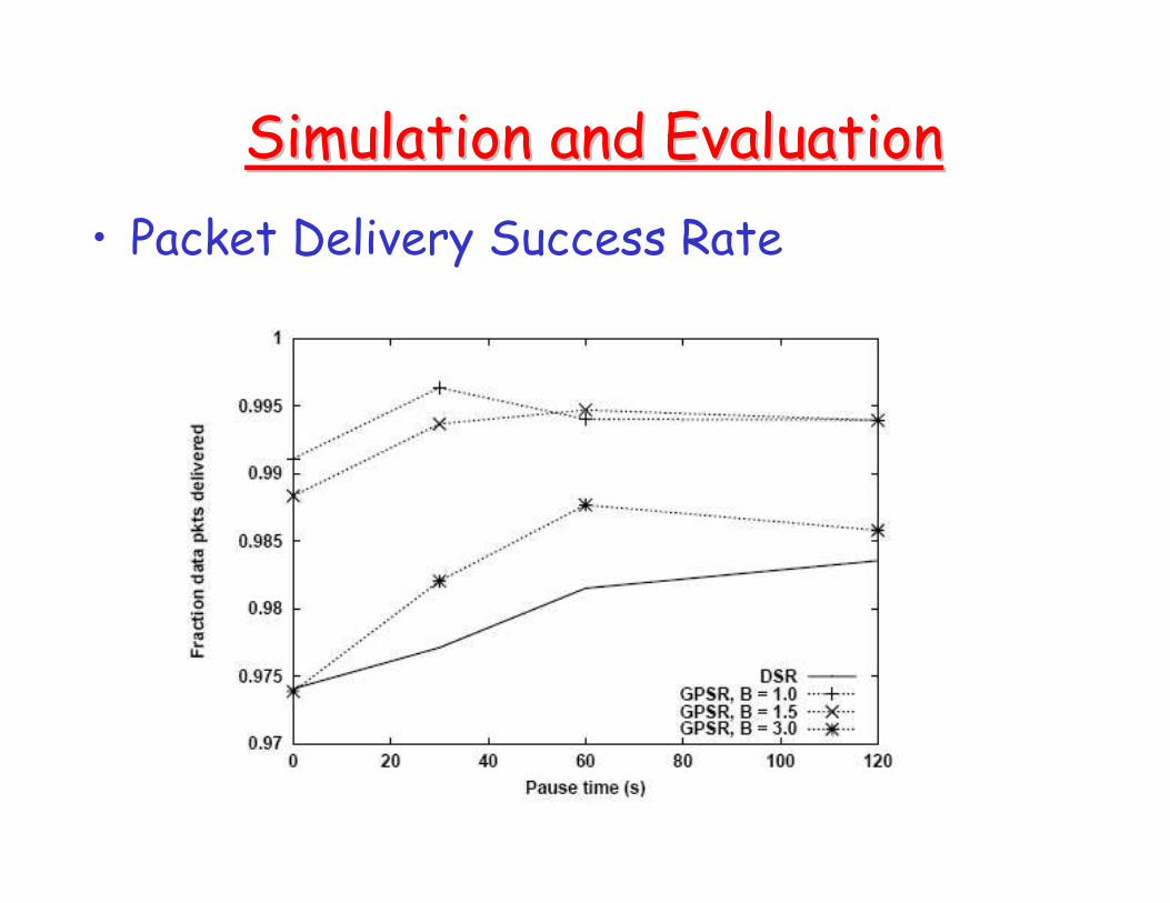
• Packet Delivery Success Rate

Simulation and EvaluationSimulation and Evaluation

• Routing Protocol Overhead

Simulation and EvaluationSimulation and Evaluation

• Path Length

Simulation and EvaluationSimulation and Evaluation

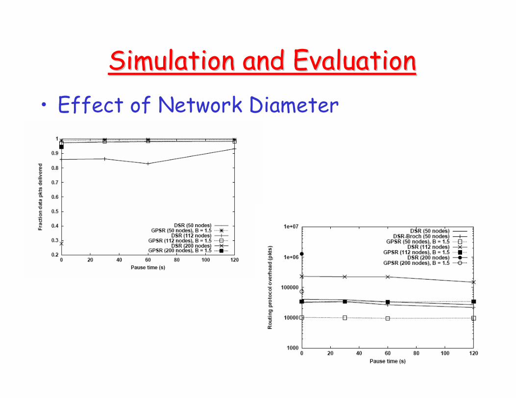
• Effect of Network Diameter

Simulation and EvaluationSimulation and Evaluation

• State per Router for 200-node – GPSR node stores state for 26 nodes on

average in pause time-0

– DSR nodes store state for 266 nodes on average in pause time-0

Simulation and EvaluationSimulation and Evaluation

Pros and Cons

• Pros:– Low routing state and control traffic � scalable

– Handles mobility

• Cons:– GPS location system might not be available

everywhere.

– Geographic distance does not correlate well with network proximity.

– Overhead in location registration and lookup

– Planarized graph is hard to guarantee under mobility

Beacon Vector RoutingBeacon Vector RoutingScalableScalable PointPoint--toto--point Routing in point Routing in

Wireless Sensor NetworksWireless Sensor Networks

R. Fonseca, S. Ratnasamy, D. Culler, S. Shenker, I. Stoica

UC Berkeley

Beacon Vector RoutingBeacon Vector Routing

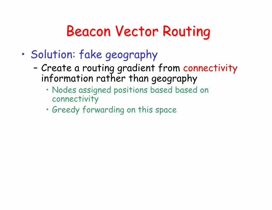
• Solution: fake geography– Create a routing gradient from connectivity

information rather than geography• Nodes assigned positions based based on

connectivity• Greedy forwarding on this space

BeaconBeacon--Vector: AlgorithmVector: Algorithm

• 3 pieces– Deriving positions

– Forwarding rules

– Lookup: mapping node IDs � positions

1. r beacon nodes (B0,B1,…,Br) flood the network; a node q’s

position, P(q), is its distance in hops to each beacon

P(q) = ⟨ B1(q), B2(q),…,Br(q) ⟩

2. Node p advertises its coordinates using the k closest beacons

(we call this set of beacons C(k,p))

3. Nodes know their own and neighbors’ positions

4. Nodes also know how to get to each beacon

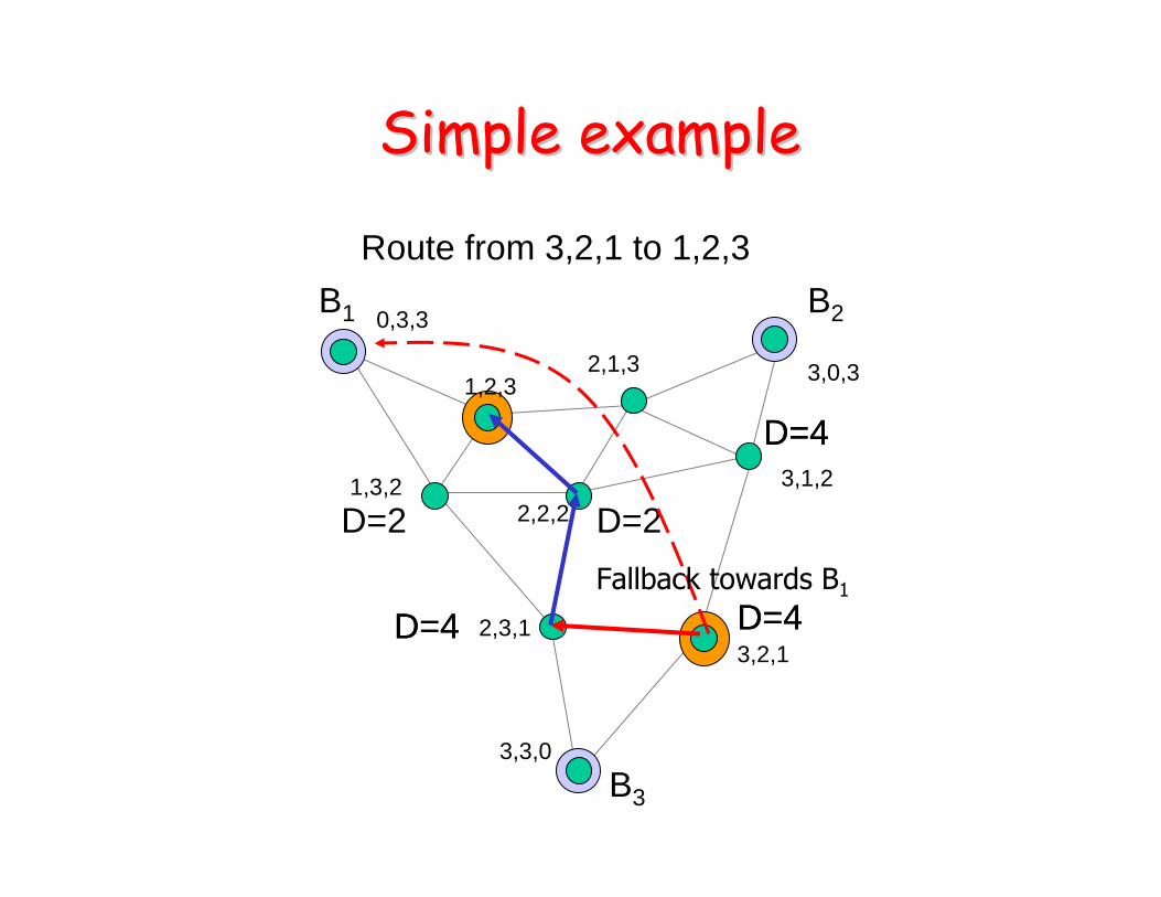
BeaconBeacon--Vector: deriving Vector: deriving positionspositions

1. Define the distance between two nodes P and Q as

2. To reach destination Q, choose neighbor to reduce distk(*,Q)

3. If no neighbor improves, enter Fallback mode: route towards the

beacon which is closer to the destination

4. If Fallback fails, and you reach the beacon, do a scoped flood

BeaconBeacon--Vector: Vector: forwardingforwarding

∑∈

−=),(

)()(),(distqkCi

iiik qBpBqp ω

Simple exampleSimple example

B1 B2

B3

1,2,3

0,3,3

2,1,3 3,0,3

3,1,21,3,2

3,3,0

2,3,13,2,1

2,2,2

Simple exampleSimple example

B1 B2

B3

1,2,3

0,3,3

2,1,3 3,0,3

3,1,21,3,2

3,3,0

2,3,13,2,1

2,2,2

Route from 3,2,1 to 1,2,3

D=4 D=4

D=4

D=2D=2

Fallback towards B1

D=4 D=4

D=4

Evaluation Evaluation -- SimulationSimulation

• Packet level simulator in C++

• Simple radio model– Circular radius, “boolean connectivity”

– No loss, no contention

• Larger scale, isolate algorithmic issues

Evaluation Evaluation -- ImplementationImplementation

• Real implementation and testing in TinyOSon mica2dot Berkeley motes

• 4KB of RAM!– Judicious use of memory for neighbor tables,

network buffers, etc

• Low power radios– Changing and imperfect connectivity– Asymmetric links– Low correlation with distance

• Two testbeds– Intel Research Berkeley, 23 motes– Soda Hall, UCB, 42 motes

Simulation ResultsSimulation Results

Effect of the number of beaconsEffect of the number of beacons

Can achieve performance comparable to that using true positions

BVR, 3200 nodes

Scaling the number of nodesScaling the number of nodesNumber of beacons needed to sustain 95% performanceNumber of beacons needed to sustain 95% performance

Beaconing overhead grows slowly with network size (less than 2% of nodes for larger networks)

Effect of DensityEffect of Density

Great benefit for deriving coordinates from connectivity, rather than positions

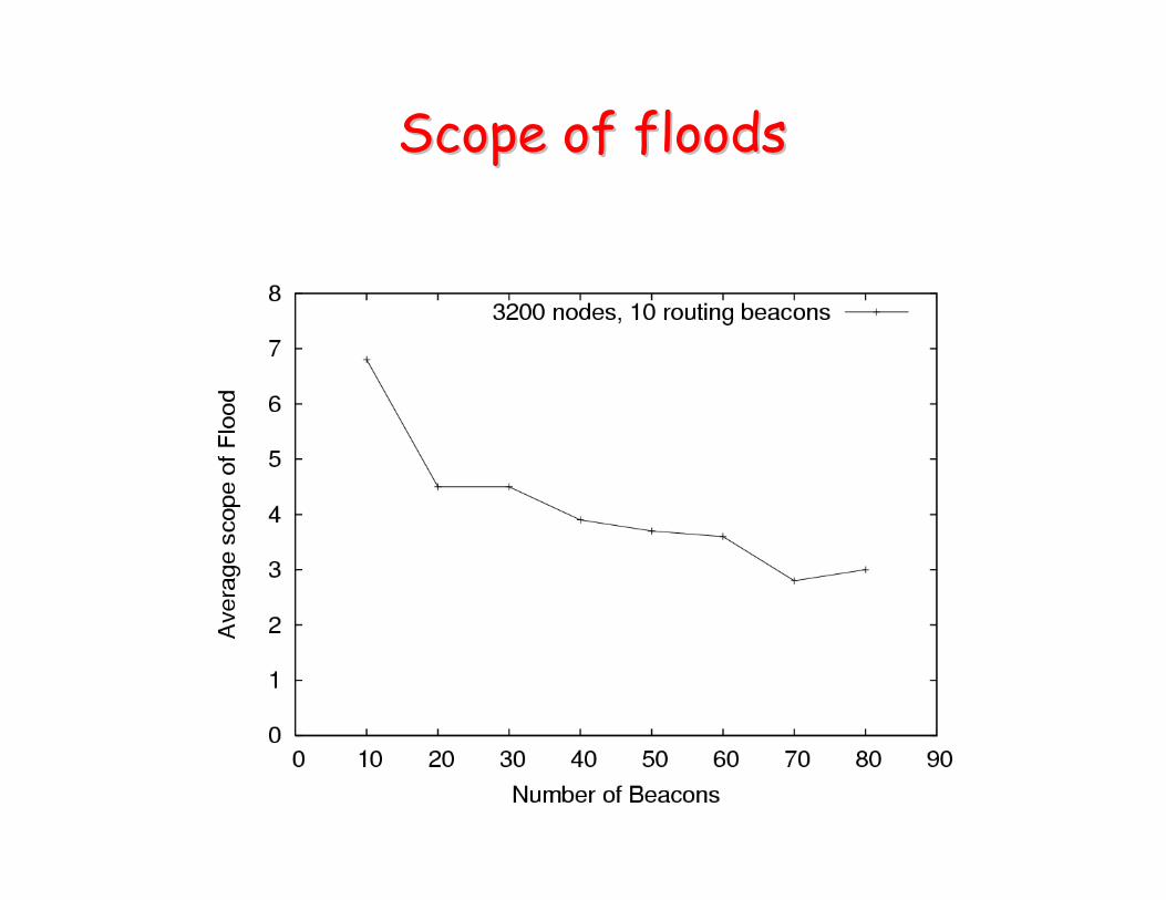
Scope of floodsScope of floods

Other results from simulationOther results from simulation

• Average stretch was consistently low– Less than 1.1 in all tests

• Performance with obstacles– Modeled as walls in the network ‘arena’

– Robust to obstacles, differently from geographic forwarding

Simulation ResultsSimulation Results

• Performance similar to that of Geographic Routing (small fraction of floods)

• Small number of beacons needed (<2% of nodes for over 95% of success rate w/o flooding)

• Scope of floods is costly

• Resilient to low density and obstacles

• Low stretch

Implementation ResultsImplementation Results

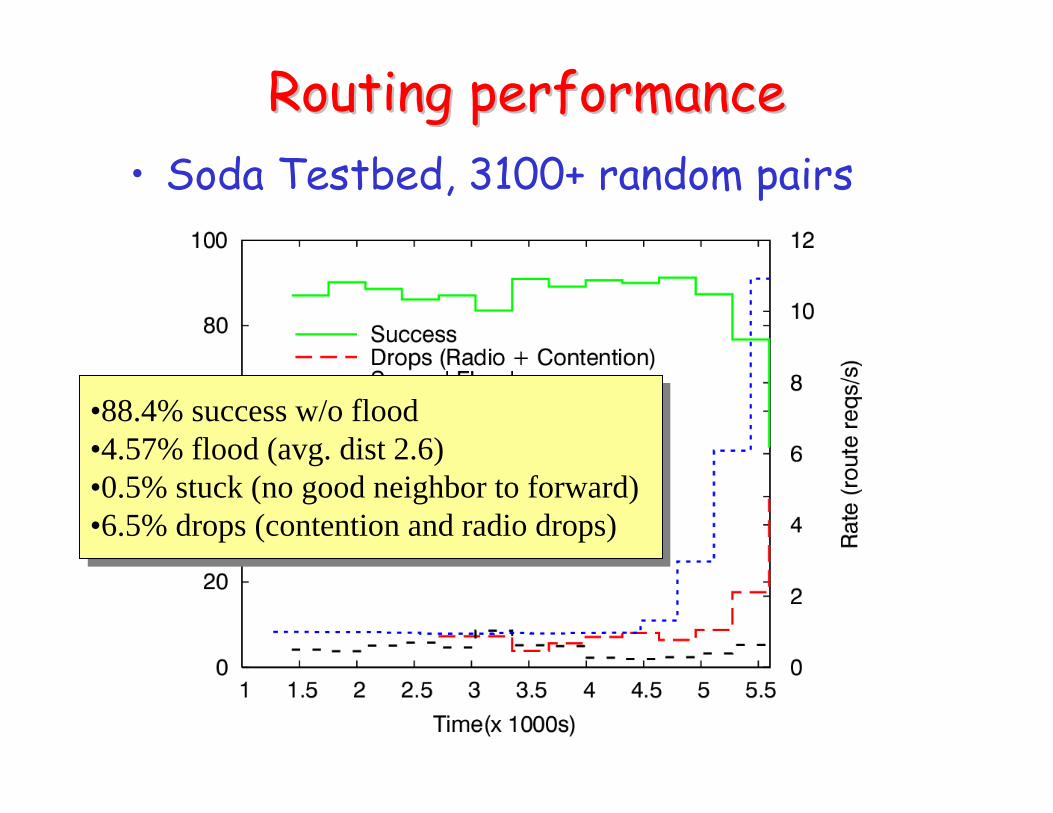
Routing performanceRouting performance

• Soda Testbed, 3100+ random pairs

•88.4% success w/o flood•4.57% flood (avg. dist 2.6)•0.5% stuck (no good neighbor to forward)•6.5% drops (contention and radio drops)

•88.4% success w/o flood•4.57% flood (avg. dist 2.6)•0.5% stuck (no good neighbor to forward)•6.5% drops (contention and radio drops)

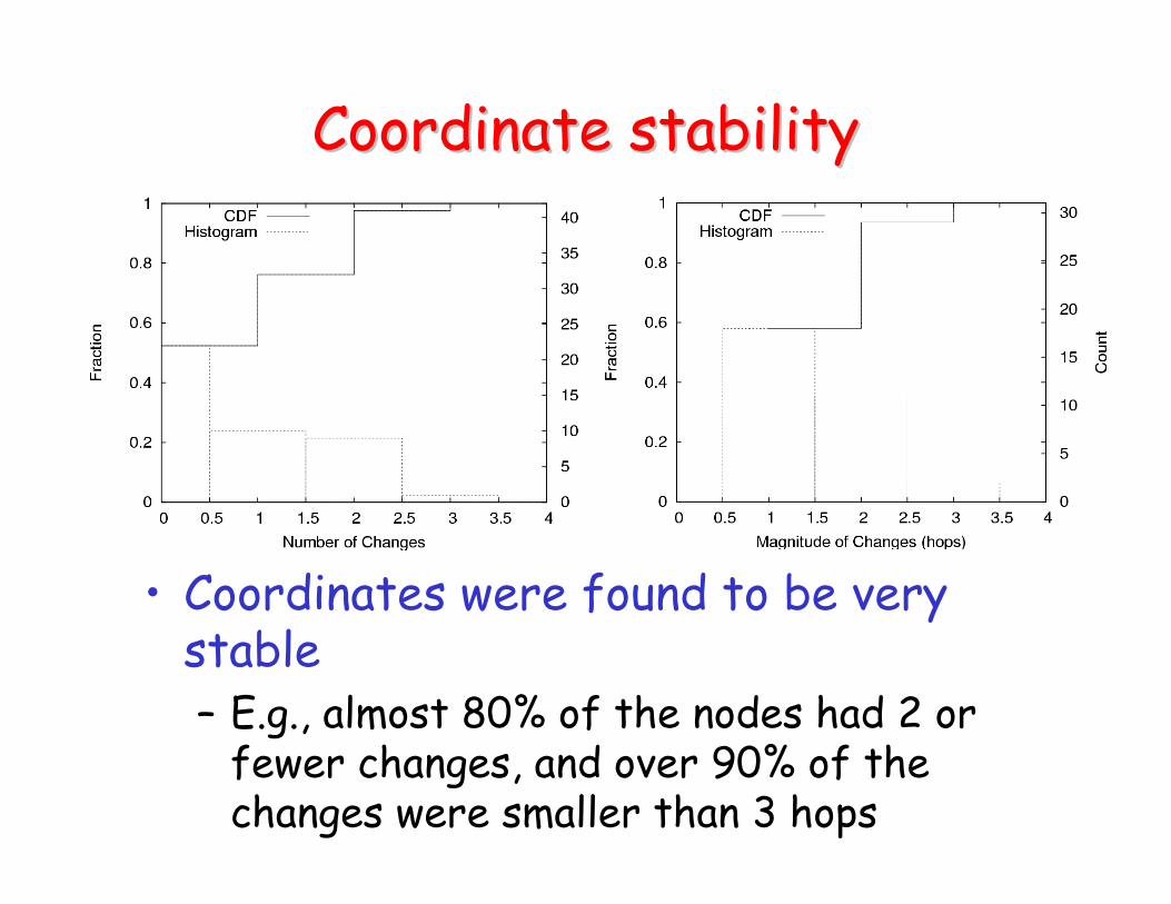
Coordinate stabilityCoordinate stability

• Coordinates were found to be very stable– E.g., almost 80% of the nodes had 2 or

fewer changes, and over 90% of the changes were smaller than 3 hops

Implementation ResultsImplementation Results

• Success rates and flood scopes agree with simulation

• Sustained high throughput (in comparison to the network capacity)

• Coordinates were found to be stable– Few changes observed, small changes

Conclusions and Future WorkConclusions and Future Work

• BVR is simple, robust to node failures, scalable, and presents efficient routes

• Using connectivity for deriving routes is good for low density/obstacles

• The implementation results indicate that it can work in real settings

• We still need to – Better study how performance is linked to radio

stability, and to high churn rates– Implement applications on top of BVR