Embed Size (px)
Citation preview

Rough Set Strategies to Data
with Missing Attribute Values
Jerzy W. Grzymala-Busse
Department of Electrical Engineering and Computer Science
University of Kansas, Lawrence, KS 66045, USA
and
Institute of Computer Science
Polish Academy of Sciences, 01-237 Warsaw, Poland
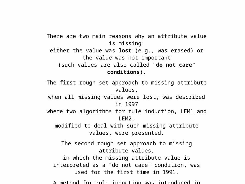
There are two main reasons why an attribute value is missing:either the value was lost (e.g., was erased) or
the value was not important(such values are also called "do not care" conditions).
The first rough set approach to missing attribute values,when all missing values were lost, was described in 1997
where two algorithms for rule induction, LEM1 and LEM2,modified to deal with such missing attribute values, were presented.
The second rough set approach to missing attribute values,in which the missing attribute value is interpreted as a "do not care"
condition, was used for the first time in 1991.
A method for rule induction was introduced in which each missing attribute value was replaced by all possible values.
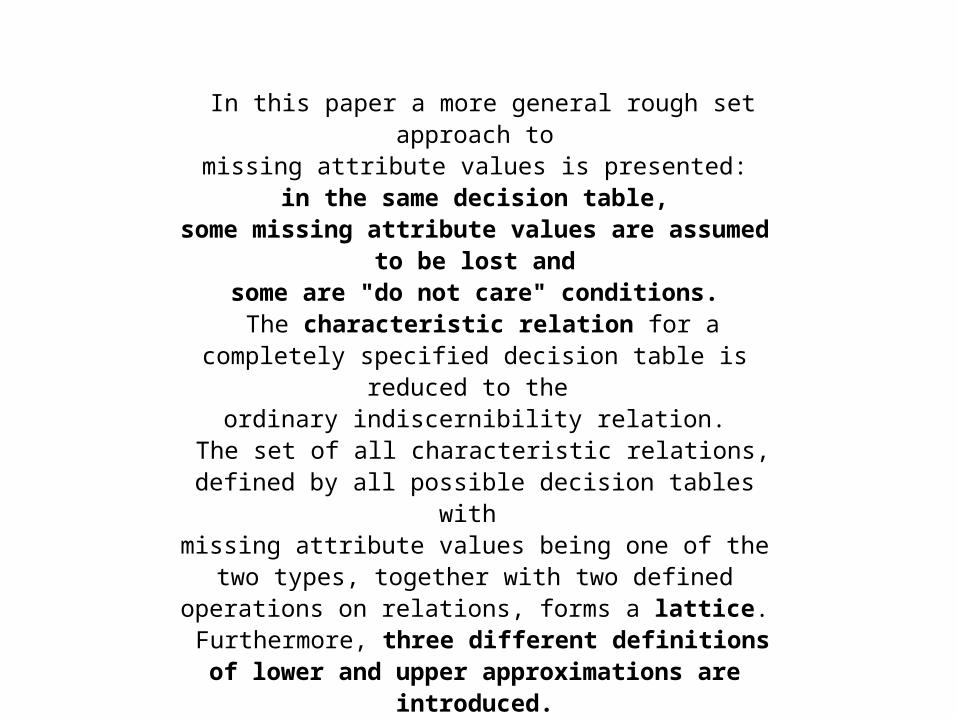
In this paper a more general rough set approach tomissing attribute values is presented:
in the same decision table,some missing attribute values are assumed to be lost and
some are "do not care" conditions.The characteristic relation for a completely specified
decision table is reduced to the ordinary indiscernibility relation.
The set of all characteristic relations,defined by all possible decision tables with
missing attribute values being one of the two types, together with two defined operations on relations, forms a lattice.
Furthermore, three different definitions of lower and upper approximations are introduced.
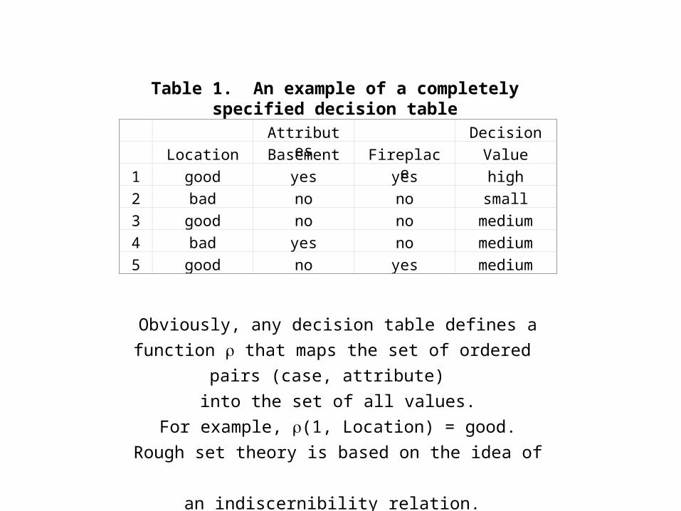
Table 1. An example of a completely specified decision table
Attributes Decision
Location Basement Fireplace Value
1 good yes yes high
2 bad no no small
3 good no no medium
4 bad yes no medium
5 good no yes medium
Obviously, any decision table defines a function that
maps the set of ordered pairs (case, attribute)
into the set of all values.
For example, (1, Location) = good.
Rough set theory is based on the idea of
an indiscernibility relation.
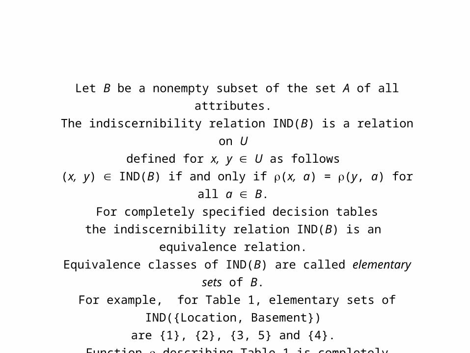
Let B be a nonempty subset of the set A of all attributes.
The indiscernibility relation IND(B) is a relation on U
defined for x, y U as follows
(x, y) IND(B) if and only if (x, a) = (y, a) for all a B.
For completely specified decision tables
the indiscernibility relation IND(B) is an equivalence relation.
Equivalence classes of IND(B) are called elementary sets of B.
For example, for Table 1, elementary sets of IND({Location, Basement})
are {1}, {2}, {3, 5} and {4}.
Function describing Table 1 is completely specified (total).
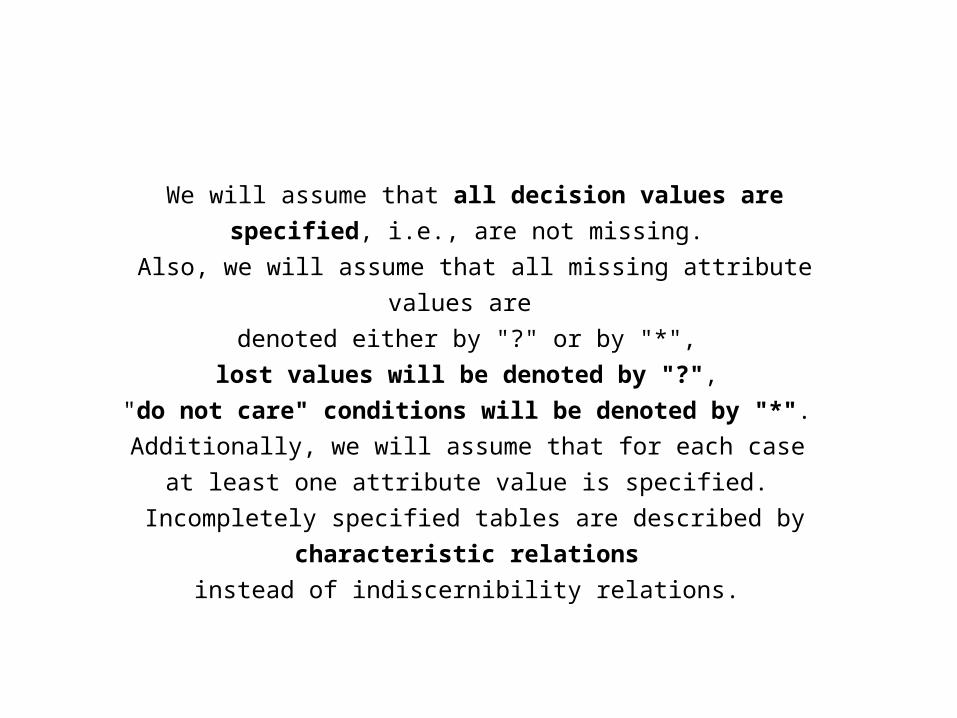
We will assume that all decision values are specified, i.e., are not missing.
Also, we will assume that all missing attribute values are
denoted either by "?" or by "*",
lost values will be denoted by "?",
"do not care" conditions will be denoted by "*".
Additionally, we will assume that for each case
at least one attribute value is specified.
Incompletely specified tables are described by characteristic relations
instead of indiscernibility relations.
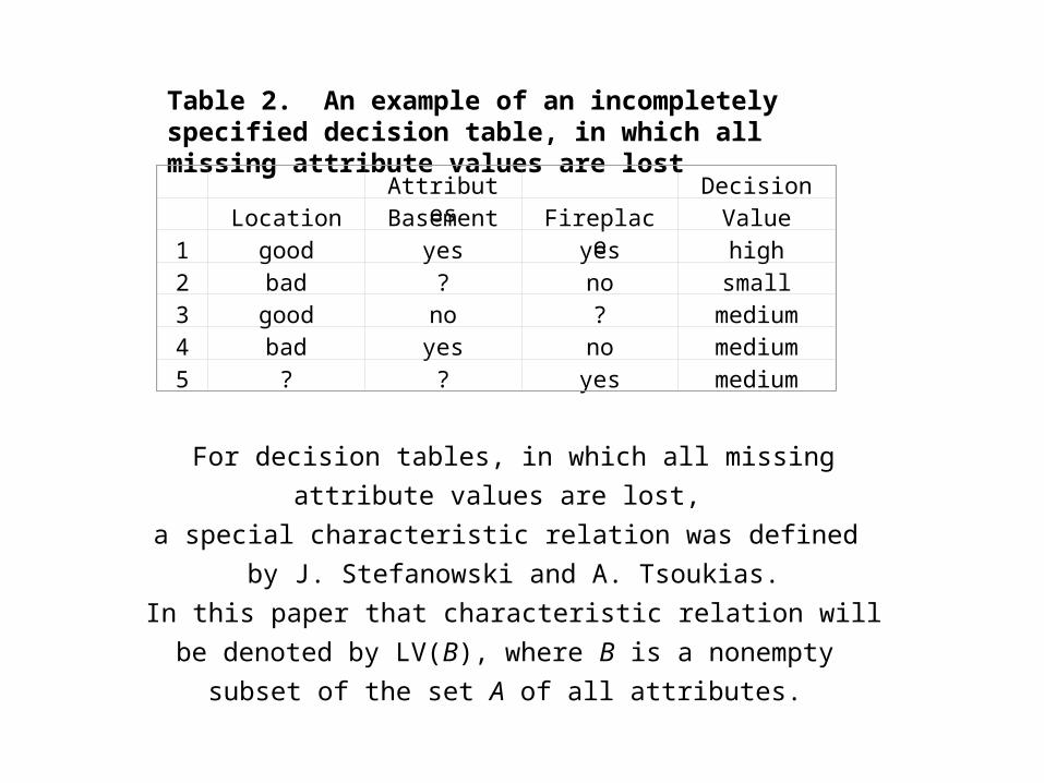
Table 2. An example of an incompletely specified decision table, in which all missing attribute values are lost Attributes Decision
Location Basement Fireplace Value
1 good yes yes high
2 bad ? no small
3 good no ? medium
4 bad yes no medium
5 ? ? yes medium
For decision tables, in which all missing attribute values are lost,
a special characteristic relation was defined
by J. Stefanowski and A. Tsoukias.
In this paper that characteristic relation will be denoted by LV(B),
where B is a nonempty subset of the set A of all attributes.

For x, y U characteristic relation LV(B) is defined as follows:
(x, y) LV(B) if and only if (x, a) = (y, a)
for all a B such that (x, a) ?.
For any case x, the characteristic relation LV(B)
may be presented by the characteristic set IB(x), where
IB(x) = {y | (x, y) LV(B)}.
For any decision table in which all missing attribute values are lost,
characteristic relation LV(B) is reflexive,
but—in general—does not need to be symmetric or transitive.
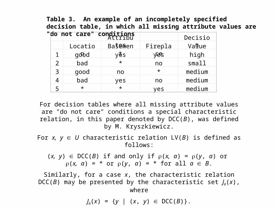
Table 3. An example of an incompletely specified decision table, in which all missing attribute values are "do not care" conditions
Attributes Decision
Location Basement Fireplace Value
1 good yes yes high
2 bad * no small
3 good no * medium
4 bad yes no medium
5 * * yes medium
For decision tables where all missing attribute values are "do not care" conditions a special characteristic relation, in this paper denoted by DCC(B), was defined by M.
Kryszkiewicz.
For x, y U characteristic relation LV(B) is defined as follows:
(x, y) DCC(B) if and only if (x, a) = (y, a) or (x, a) = * or (y, a) = * for all a B.
Similarly, for a case x, the characteristic relation DCC(B) may be presented by the characteristic set JB(x), where
JB(x) = {y | (x, y) DCC(B)}.
Relation DCC(B) is reflexive and symmetric but—in general—not transitive.

Table 4. An example of an incompletely specified decision table, in which some missing attribute values are lost and some are "do not care" conditions
Attributes Decision
Location Basement Fireplace Value
1 good yes yes high
2 bad ? no small
3 good no ? medium
4 bad yes no medium
5 * * yes medium
A characteristic relation R(B) on U foran incompletely specified decision table with both types
of missing attribute values: lost values and "do not care" conditions:(x, y) R(B) if and only if (x, a) = (y, a) or (x, a) = * or (y, a) = * for all a B such that (x, a) = ?,
where x, y U and B is a nonempty subset of the set A of all attributes.For a case x, the characteristic relation R(B) may be also presented by its characteristic set KB(x),
where KB(x) = {y | (x, y) R(B)}.
Characteristic relations LV(B) and DCC(B) are special cases ofthe characteristic relation R(B).
For a completely specified decision table, the characteristic relation R(B) is reduced to IND(B).The characteristic relation R(B) is reflexive but—in general—does not need to be symmetric or transitive.
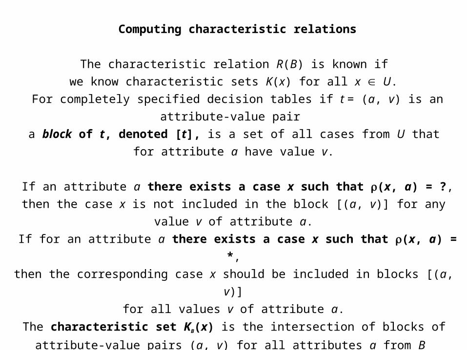
Computing characteristic relations
The characteristic relation R(B) is known if
we know characteristic sets K(x) for all x U.
For completely specified decision tables if t = (a, v) is an attribute-value pair
a block of t, denoted [t], is a set of all cases from U that
for attribute a have value v.
If an attribute a there exists a case x such that (x, a) = ?,
then the case x is not included in the block [(a, v)] for any value v of attribute a.
If for an attribute a there exists a case x such that (x, a) = *,
then the corresponding case x should be included in blocks [(a, v)]
for all values v of attribute a.
The characteristic set KB(x) is the intersection of blocks of
attribute-value pairs (a, v) for all attributes a from B
for which (x, a) is specified and (x, a) = v.
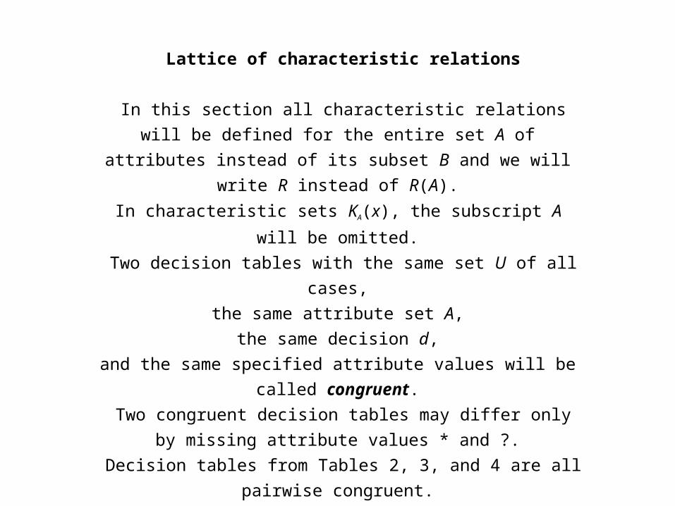
Lattice of characteristic relations
In this section all characteristic relations will be defined for the entire
set A of attributes instead of its subset B and we will write R instead of
R(A).
In characteristic sets KA(x), the subscript A
will be omitted.
Two decision tables with the same set U of all cases,
the same attribute set A,
the same decision d,
and the same specified attribute values will be called congruent.
Two congruent decision tables may differ only
by missing attribute values * and ?.
Decision tables from Tables 2, 3, and 4 are all pairwise congruent.
Two congruent decision tables that have
the same characteristic relations will be called indistinguishable.
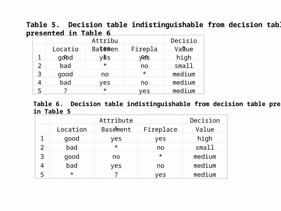
Table 5. Decision table indistinguishable from decision table presented in Table 6 Attributes Decision
Location Basement Fireplace Value1 good yes yes high2 bad * no small3 good no * medium4 bad yes no medium5 ? * yes medium
Table 6. Decision table indistinguishable from decision table presented in Table 5 Attributes Decision
Location Basement Fireplace Value
1 good yes yes high
2 bad * no small
3 good no * medium
4 bad yes no medium
5 * ? yes medium

On the other hand, if the characteristic relations for two congruent decision tables are
different, the decision tables will be called distinguishable.
Obviously, there is 2n congruent decision tables, where n is the total number of all
missing attribute values in a decision table.
Let D1 and D2 be two congruent decision tables,
let R1 and R2 be their characteristic relations,
and let K1(x) and K2(x) be their characteristic sets for some x U, respectively.
We say that R1 R2 if and only if K1(x) K2(x) for all x U.
For two congruent decision tables D1 and D2, D1 D2
if for every missing attribute value"?" in D2, say 2(x, a),
the missing attribute value for D1 is also "?",
i.e., 1(x, a), where 1 and 2 are functions defined by D1 and D2, respectively.
Two subsets of the set of all congruent decision tables are special:
set E of n decision tables such that every decision table from E
has exactly one missing attribute value "?"
and all remaining attribute values equal to "*" and
the set F of n decision tables such that every decision table from E
has exactly one missing attribute value "*" and all remaining
attribute values equal to "?".
In our example, decision tables presented in Tables 5 and 6
belong to the set E.
Let G be the set of all characteristic relations associated with the set E and
let H be the set of all characteristic relations associated with the set F.

Let D and D' be two congruent decision tables with characteristic relations R and R', and with characteristic sets K(x) and K'(x), respectively,
where x U.
We define a characteristic relation R + R' as defined by characteristic sets K(x) K'(x), for x U,
and a characteristic relation RR' as defined by characteristic sets K(x)K'(x).
The set of all characteristic relations for the set of all congruent tables, together with operations + and , is a lattice L
(i.e., operations + and satisfy the four postulates of idempotent, commutativity, associativity, and absorption laws).
Each characteristic relation from L can be represented(using the lattice operations + and )
in terms of characteristic relations from G (and, similarly for H).
Thus G and H are sets of generators of L.

The diagram of the lattice of all characteristic relations

Lower and upper approximations
For completely specified decision tables lower and upper
approximations are defined on the basis of the indiscernibility
relation.
An equivalence class of IND(B) containing x is denoted by
[x]B.
Any finite union of elementary sets of B is called a
B-definable set.
Let U be the set of all cases, called an universe.
Let X be any subset of U.
The set X is called concept and is usually defined as the set
of all cases defined by specific value of the decision.
In general, X is not a B-definable set.

However, set X may be approximated by two B-definable sets,the first one is called a B-lower approximation of X and defined as follows
{x U | [x]B X }.
The second set is called an B-upper approximation of X and defined as follows
{x U | [x]B X }.
The B-lower approximation of X is the greatest B-definable set, contained in X.
The B-upper approximation of X is the least B-definable set containing X.
For incompletely specified decision tables
lower and upper approximations may be defined in a few different ways.

Let X be a concept,let B be a subset of the set A of all attributes,
and let R(B) be the characteristic relation of the incompletely specified decision table with characteristic sets K(x), where x U.
Our first definition uses a similar idea as in the previous articles on incompletely specified decision tables, i.e., lower and upper
approximations are sets of singletons from the universe U satisfying some properties.
We will call these definitions singleton.A singleton B-lower approximation of X is defined as follows:
{x U | KB(x) X }.
A singleton B-upper approximation of X is{x U | [x]B X }.
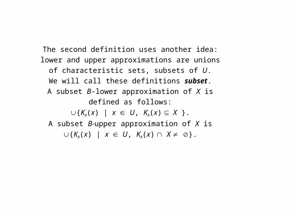
The second definition uses another idea: lower and upper
approximations are unions of characteristic sets, subsets of U.
We will call these definitions subset.
A subset B-lower approximation of X is defined as follows:
{KB(x) | x U, KB(x) X }.
A subset B-upper approximation of X is
{KB(x) | x U, KB(x) X }.

The next possibility is to modify the subset definition
of upper approximation
by replacing the universe U from the previous definition
by a concept X.
A concept B-lower approximation of the concept X is
defined as follows:
{KB(x) | x X, KB(x) X }.
Obviously, the subset B-lower approximation of X is the
same set as the concept B-lower approximation of X.
A concept B-upper approximation of the concept X is
defined as follows:
{KB(x) | x X, KB(x) X }.

Some properties that hold for singleton lower and upper
approximations do not hold—in general—for subset lower
and upper approximations and for concept lower and upper
approximations.
For example, for singleton lower and upper approximations
{x U | IB(x) X } {x U | JB(x) X }
and
{x U | IB(x) X ¯ } {x U | JB(x) X ¯ },
where IB(x) is a characteristic set of LV(B) and
JB(X) is a characteristic set of DCC(B).

In our example, for the subset definition of A-upper approximation,X = {3, 4, 5}, and the characteristic relation LV(A) (see Table 2)
{IB(x) | IB(x) X } = {3, 4}
while for the subset definition of A-upper approximation,
X = {3, 4, 5}, and the characteristic relation DCC(A) (see Table 3)
{JB(x) | JB(x) X } = {3, 5},
so neither the former set is a subset of the latter nor vice versa
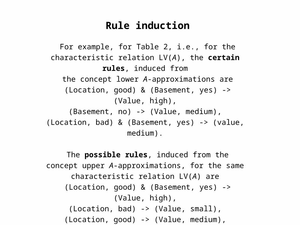
Rule induction
For example, for Table 2, i.e., for the characteristic relation
LV(A), the certain rules, induced from
the concept lower A-approximations are
(Location, good) & (Basement, yes) -> (Value, high),
(Basement, no) -> (Value, medium),
(Location, bad) & (Basement, yes) -> (value, medium).
The possible rules, induced from the concept upper A-
approximations, for the same characteristic relation LV(A) are
(Location, good) & (Basement, yes) -> (Value, high),
(Location, bad) -> (Value, small),
(Location, good) -> (Value, medium),
(Basement, yes) -> (Value, medium),
(Fireplace, yes) -> (Value, medium).
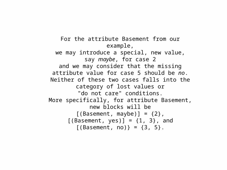
For the attribute Basement from our example,we may introduce a special, new value,
say maybe, for case 2and we may consider that the missing attribute value for case 5
should be no.Neither of these two cases falls into the category of lost values
or"do not care" conditions.
More specifically, for attribute Basement, new blocks will be[(Basement, maybe)] = {2},
[(Basement, yes)] = {1, 3}, and[(Basement, no)} = {3, 5}.

Conclusions
The existing two approaches to missing attribute values,
interpreted as a lost value or as a "do not care" condition
are generalized by interpreting every
missing attribute value separately as a lost value or
as a "do not care" condition.
Characteristic relations are introduced to describe
incompletely specified decision tables.
Lower and upper approximations
for incompletely specified decision tables
may be defined in a variety of different ways.