Rotorcraft Linear Simulation Model Final Report

NASA CR 152079

Rotorcraft Linear Simulation Model Final Report

Volume II. Computer Implementation

By J. S.REASER D. H. SAIKI

January 1978

Distribution of this report is provided in the interest of information exchange. Responsibility for. the contents resides in the author or

organization that prepared it. " (NAS A-CR- 152,079-Vol- 2) pO ORCIRAFT V1 VE A IR8-

SSIMUIATION MODE1. VOUME 2:" CONEWTEE IIPLENENTATION Final Report, Nov- 1976

[Burbank.) 777 p HC A05/MT 0 CCL 01C G3/08-'11047 j

Prepared under Contract No. NAS2-9374 by LOCKHEED-CALIFORNIA COMPANY

P. 0. Box 551 Burbank, California 91520

i A'[Pi978 ,

for

AMES RESEARCH CENTER NATIONAL AERONAUTICS AND SPACE ADMINISTRATION

Moffett Field, California 94035

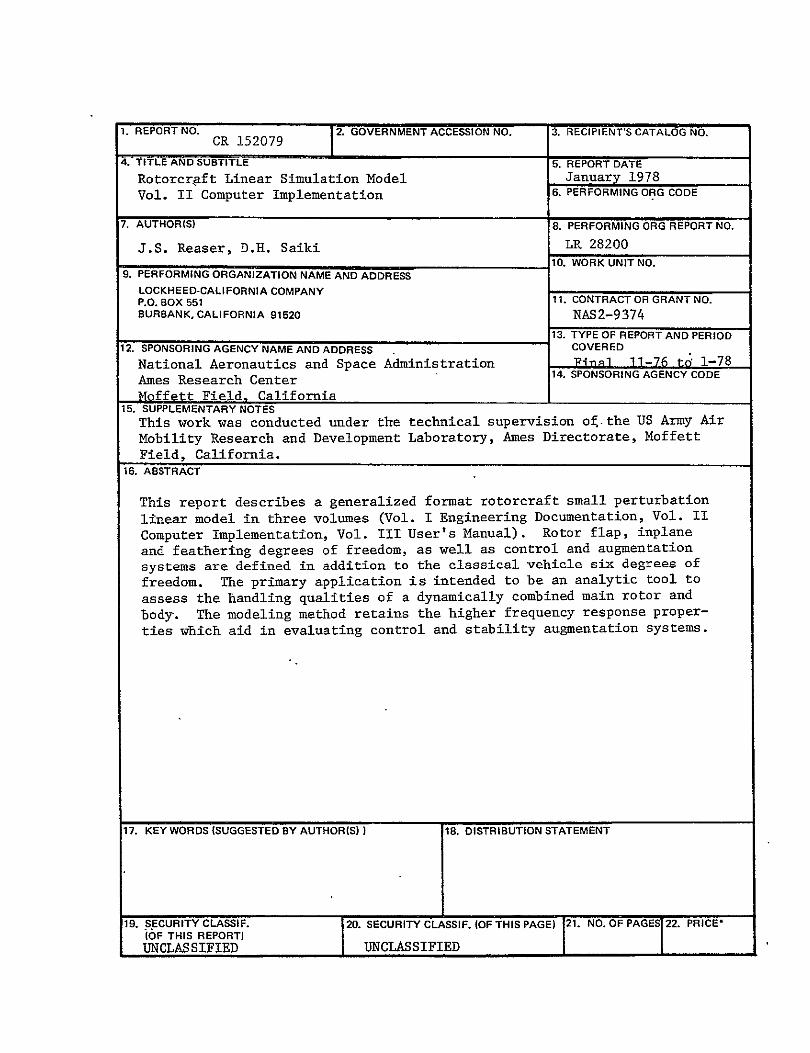
1. REPORT NO. | 2. GOVERNMENT ACCESSION NO. 3. RECIPIENT'S CATALOG NO.ICR 152079

4.-fTLE AND SUBTITLE 5. REPORT DATE

Rotorcraft Linear Simulation Model January 1978

Vol. II Computer Implementation 6. PERFORMING ORG CODE

7. AUTHOR(S) 8. PERFORMING ORG REPORT NO.

LR 28200J.S. Reaser, D.H. Saiki 10. WORK UNIT NO.

9. PERFORMING ORGANIZATION NAME AND ADDRESS

LOCKHEED-CALIFORNIA COMPANY P.O. BOX 551 11. CONTRACT OR GRANT NO. BURBANK, CALIFORNIA 91520 NAS2-9374

13. TYPE OF REPORT AND PERIOD

12. SPONSORING AGENCY NAME AND ADDRESS COVERED

1-7 8 National Aeronautics and Space Administration IFinal 11-76 to 14. SPONSORING AGENCY CODEAmes Research Center

Moffett Field, California 15. SUPPLEMENTARY NOTES

This work was conducted under the technical supervision of- the US Army Air

Mobility Research and Development Laboratory, Ames Directorate, Moffett Field, California.

16. ABSTRACT

This report describes a generalized format rotorcraft small perturbation

linear model in three volumes (Vol. I Engineering Documentation, Vol. II

Computer Implementation, Vol. III User's Manual). Rotor flap, inplane

and feathering degrees of freedom, as well as control and augmentation

systems are defined in addition to the classical vehicle six degrees of

freedom. The primary application is intended to be an analytic tool to

assess the handling qualities of a dynamically combined main rotor and

body. The modeling method retains the higher frequency response proper

ties which aid in evaluating control and stability augmentation systems.

17. KEY WORDS (SUGGESTED BY AUTHOR(S) ) 18. DISTRIBUTION STATEMENT

19. SECURITY CLASSIF. 20. SECURITY CLASSIF. IOF THIS PAGE) 21. NO. OF PAGES 22. PRICE* (OF THIS REPORT] UNCLASSIFIED UNCLASSIFIED

FOREWORD

This report describes a generalized rotorcraft small perturbation, linear

model and associated computer software which have been refined and documented

for NASA, Ames Research Center, Moffett Field, California, under contract

NAS2-9374 (November, 1976) as ammended Revision (1) (May, 1977). This work

has been performed by the Lockheed-California Company, Burbank, California.

Dr. R.T.N. Chen of the Ames Directorate, U.S. Army Air Mobility Research

and Development Laboratory (USAAMRDL) was the technical monitor for this

project. P.H. Kretsinger, D.H. Saiki and H.P. Weinberger (all of Lockheed-

California Company) performed the software implementation of the linear model

and matrix processing routines. A. J. Potthast and Fox Conner (also Lockheed

personnel) provided technical assistance and technical editing of the

documentation.

TABLE OF CONTENTS

Section Page

LIST OF ILLUSTRATIONS vii

LIST OF TABLES ix

SUMMARY 1

SYMBOLS 3

1 PACKAGE ORGANIZATION 15

1.1 FLOW CHART 15

1.2 OPERATION MODES 15

1.2.1 Trim 17

1.2.2 Derivatives 17

1.2.3 Matrix Formulation 17

1.2.4 Control Systems Analysis Package (CSAP) 17

1.2.4.1 Modes of Operation 18

1.2.4.2 Matrix Operations 18

1.2.4.2.1 Formation of the state matrix 18

1.2.4.2.2 QR double iteration 21

1.2.4.2.3 Definition of the QR iteration 21

1.2.4.2.4 The double QR iteration 22

1.2.4.3 Output Description 23

1.2.4.4 Data Storage -24

1.3 SUBROUTINES 25

1.3.1 CPUNCH 26

1.3.2 DERIVE 26

1.3.3 DPQFB 27

1.3.4 DPRBM 29

1.3.5 EIGVAL 30

1.3.6 EIGVEC 31

1.3.7 FREQR 32

illi

TABLE OF CONTENTS (CONT)

Section Page

1.3.8 GELG 34

1.3.9 HSBGNM 35

1.3.10 INFLOW 36

1.3.11 MAIN 36

1.3.12 MATRIX 37

1.3.13 MODEL 38

1.3.14 NWMTRX 38

1.3.15 PDATE 39

1.3.16 PKDATA 40

1.3.17 PLXDIV 41

1.3.18 PLYFRM 41

1.3.19 POLRT 42

1.3.20 POWER 43

1.3.21 PRINT 45

1.3.22 PRINTR 46

1.3.23 PROD 47

1.3.24 QR 48

1.3.25 RDMTRX 49

1.3.26 READIN 51

1.3.27 ROOT 51

1.3.28 RTEST 52

1.3.29 RTPOLY 53

1.3.30 STMTEX 54

1.3.31 TIMEN 55

1.3.32 TRIM 58

1.3.33 VECTOR 59

1.3.34 XMAX 60

1.3.35 XMIN 61

1.3.36 XPLOT 61

1.3.37 YPLOT 62

1.3.38 ZPLOT 62

iv

TABLE OF CONTENTS (CONT)

Section Page

2 COMMON/SUBROUTINE DIRECTORY 63

3 COMPLETE SOURCE LISTING 68

4 REFERENCES 69

v

kREWD=NQ PAGE BL-AK NT-FUM

LIST OF ILLUSTRATIONJS

Figure

1-1 Linear Model Flow Chart

1-2 Time History Integrator Format 16

2-1 Linear Model Subroutine Hierarchy 57

64

vii

IMXMMING PAGB BLAN& NWT MI'fA

LIST OF TAsLEs

Table

21 2-2

Subroutlne Directory7gCOVOl D iretory

65

67

Ix

ROTORCRAFT LINEAR SIMULATION MODEL

Volume II. Computer Implementation

J.S. Reaser D.H. Saiki

Lockheed-California Company

SUMMARY

- This report describes a generalized format rotorcraft small perturbation

linear model. Rotor flap, inplane and feathering degrees of freedom, as well

as control and augmentation systems are defined in addition to the classical

vehicle six degrees of freedom. The model simulates a single main rotor air

craft although it can be readily expanded to simulate compound aircraft with

auxiliary thrust and wings. The analysis concept can also be expanded to

model multiple lifting rotor configurations.

This report is divided into three volumes. The first volume contains the

development of rotorcraft mechanical and aerodynamic equations. The second

volume presents the description of a computer program that can be used to

process the equations. The third volume contains the computer program

operating instructions and defines the input-output data format.

The model development and application assumes that the main rotor control

power, i.e., body moment due to blade flapping, has been established analytically

or experimentally. These data are used to define the equivalent spring rate

of the main rotor to body coupling.

The primary application is intended to be an analytic tool to assess the

handling qualities of a dynamically combined main rotor and body. To this end,

the rotor degrees of freeaom appear explicitly rather than being included in

the classical six degrees of freedom through a quasi-steady reduction process.

The higher frequency response properties of the rotor are retained, and appear

in the handling qualities assessment. Control and stability augmentation sys

tems are therefore evaluated more realistically. The model does not address

the area of rotor dynamic stability.

The model has been implemented in IBM 360 and CDC 7600 series computer

systems. The IBM 360 implementation includes graphic as well as tabulated

output capability.

2

SYMBOLS

a -rotor blade section lift slope, rad - 1

aHT horizontal tail lift slope, rad - I

aVT vertical tail lift slope, rad - I

a. wing-body lift slope, rad-1

a blade collective flap up angle, rad

a1 longitudinal flap (up, forward) angle, rad

A area, ft 2; blade span axis

A1 longitudinal feather (nose up, forward) angle, rad

AR aspect ratio

b wing span, ft

bI lateral flap (down, right) angle, rad

B dissipation function, ft-lb/sec; tip loss factor; body

subscript; blade subscript; blade chord (aft) axis

B1 lateral feather (nose down, right) angle, rad

3

c cosine component subscript; blade element chord, ft; wing

chord, ft

o wing mean chord, ft

o blade vertical (down) axis

CD drag coefficient

C D drag coefficient, input value

control gyro fixed coordinate damping rate, ft ib/rad/secCF

lift coefficientCL

CM pitching moment coefficient

control gyro rotating coordinate damping rate, ft ib/rad/secCR

C Y body-wing side force coefficient

CG center-of-gravity subscript

(a)R nondimensional rotor thrust, disc axis

torque, shaft axis nondimensional rotor ()R rotor drag, shaft axis nondimensional()R

C6 c cosine axis cyclic fixed system damping rate, ft ib/rad/sec

C65c cross axis cyclic fixed system damping rate, ft lb/rad/secs

4

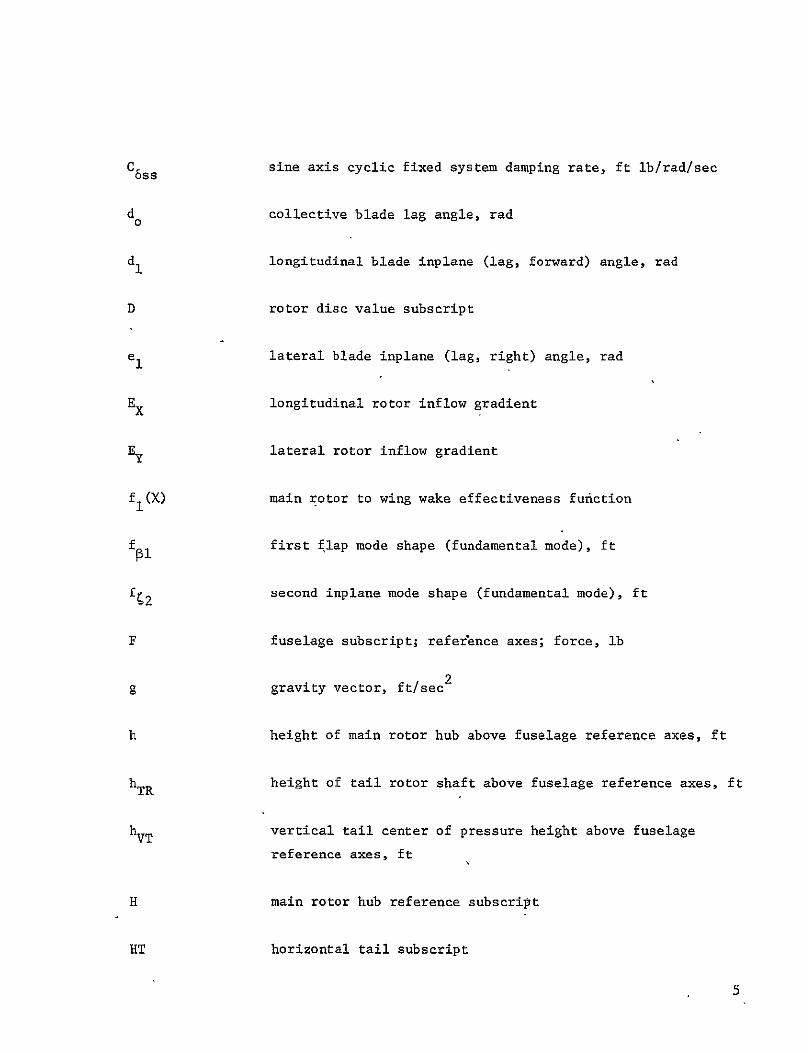
C5ss sine axis cyclic fixed system damping rate, ft lb/rad/sec

d collective blade lag angle, rad

d 1 longitudinal blade inplane (lag, forward) angle, rad

D rotor disc value subscript

e1 lateral blade inplane (lag, right) angle, rad

EX longitudinal rotor inflow gradient

Flateral rotor inflow gradient

f1(W main rotor to wing wake effectiveness function

flifirst flap mode shape (fundamental mode), ft

f 2 second inplane mode shape (fundamental mode), ft

F fuselage subscript; referlence axes; force, lb

g gravity vector, ft/sec2

h height of main rotor hub above fuselage reference axes, ft

hTR height of tail rotor shaft above fuselage reference axes, ft

hvT vertical tail center of pressure height above fuselage

reference axes, ft

H main rotor hub reference subscript

HT horizontal tail subscript

5

i induced value subscript

IA blade feathering moment of inertia about the feathering

hinge, slug ft2

IAB blade flap-chord product of inertia about flap and feathering

hinges, slug ft2

IAC blade inplane-chord product of inertia about inplane and feathering hinges, slug ft2

IB blade flap moment of inertia about flap hinge, slug ft2

blade inplane moment of inertia about inplane hinge, slug 2

ft

IsP blade flap-inplane product of inertia about flap and inplane

hinges, slug ft2

IXX helicopter roll moment of inertia, slug ft2

IXZ helicopter roll-yaw product of inertia, slug ft2

pitch moment of inertia, slug ft2

IyYYhelicopter

IZ helicopter yaw moment of inertia, slug ft2

K spring rate (general), ft ib/rad

"KF control gyro fixed coordinate spring rate, ft lb/rad

"KFB flap feedback spring rate, ft lb/rad

6

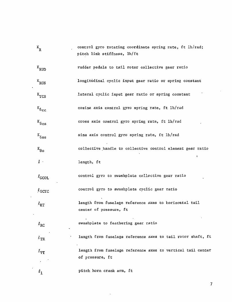
KR control gyro totating coordinate spring rate, ft ib/rad;

pitch link stiffness, lb/ft

KRUD rudder pedals to tail rotor collective gear ratio

KxCS longitudinal cyclic input gear ratio or spring constant

\CS lateral cyclic input gear ratio or spring constant

K6cc cosine axis control gyro spring rate, ft ib/rad

K cs cross axis control gyro spring rate, ft lb/rad

K6ss sine axis control gyro spring rate, ft ib/rad

KGO collective-handle to collective control element gear ratio

" length, ft

2GCOL control gyro to swashplate collective gear ratio

IGCYC control gyro to swashplate cyclic gear ratio

2HT length from fuselage reference axes to horizontal tail

center of pressure, ft

2RC swashplate to feathering gear ratio

2TR length from fuselage reference axes to tail rotor shaft, ft

2VT length from fuselage reference axes to vertical tail center

of pressure, ft

2i pitch horn crank arm, ft

7

R2 swashplate crank arm, ft

R3 pitch-flap coupling arm, ft

R4 pitch-lag coupling arm, ft

L aircraft rolling moment, ft lb

m blade element mass, slug/ft

M aircraft mass, slugs; aircraft pitching moment, ft lb

MLIF blade flap-radius moment of inertia, slug ft2

MR main rotor subscript

MY blade feathering mass moment, slug ft

MIF blade flap mass moment, slug ft

M2L blade inplane mass moment, slug ft

MPe cosine blade flapping moment, ft lb

Mo coning moment, ft lb

Mps sine blade flapping moment, ft lb

M~c cosine blade inplane moment, ft lb

% sine blade inplane moment, ft lb

DMr/t blade inplane damping, ft ib/rad/sec

8

N number of blades; aircraft yawing moment, ft lb

0 initial value subscript; root value subscript; steady

component subscript

p instantaneous roll rate, rad/sec

P0 initial roll rate, rad/sec

q instantaneous pitch rate, rad/sec; generalized coordinate

Q generalized force

blade root flapping potential energy, ft lb

QEe

QE

Qo

blade root feathering potential energy, ft lb

blade root inplane potential energy, ft lb

initial pitch rate, rad/sec

QK rotor shaft torque, ft lb

r instantaneous yaw rate, rad/sec; blade radial distance, ft

R main rotor blade radius, ft; rotor subscript

R o initial yaw rate, rad/sec

s

S

SHT

sine component subscript

shaft axes subscript; area, ft2

horizontal tail area, ft2

9

SVT vertical tail area, ft2

SW wing area, ft2

T kinetic energy, ft ib; rotor thrust, lb

TTR tail rotor thrust, lb

TR tail rotor subscript

u instantaneous longitudinal velocity, ft/sec

U potential energy function, ft lb

U initial longitudinal velocity, ft/sec

v instantaneous lateral velocity, ft/sec

V0 initial lateral velocity, ft/sec

VT trajectory velocity, ft/sec

w instantaneous vertical velocity, ft/sec

W work function, ft lb; wing subscript

W initial vertical velocity, ft/sec

x nondimensional blade element radial position

X instantaneous longitudinal axis

X longitudinal aft stick deflection

10

X0

y

initial longitudinal axis

blade element chordwise position to trailing edge, ft

YTR

Y

tail rotor hub lateral offset to

instantaneous lateral axis

right, ft

Y cs

Y 0

Z

lateral right stick deflection

initial lateral axis

instantaneous vertical (down) axis

Zo

a

initial

angle

vertical (down)

of atack, rad

axis

qs shaft angle of attack, rad

a2

pblade

pitch-lag coupling

flapping up deflection, rad

PDR

Ps

blade droop from feather axis, rad

side slip angle, rad

y climb angle, rad

6 control gyro up deflection, red; infinitesimal increment

6c cosine component control gyro deflection, rad

11

8o collective component control gyro deflection, rad

6s sine component control gyro deflection, rad

63 pitch-flap coupling

Aswashplate up deflection, rad

Ac cosine component swashplate deflection, rad

AO collective component swashplate deflection, rad

AS sine component swashplate deflection, rad

E wake angle function, rad

blade inplane lag deflection, rad

SW blade root sweep forward, rad

load factor

E pitch euler angle, rad; blade feathering motion, rad;

3/4 radius collective angle, rad

Go root collective angle, rad; initial pitch attitude, rad

Xo nondimensional disc total inflow

Xi nondimensional induced inflow

XD nondimensional disc plane inflow

ks nondimensional shaft total inflow

12

A nofidimensional rotor total vector velocity

velocity normalized to rotor 'tip speed, nondimensional

vector nondimensional velocity

1p blade element nondimensional perpendicular velocity

LT blade element nondimensional tangential velocity

ILX nondimensional forward velocity, reference axis system

Iy nondimensional right velocity, reference axis system

Z nondimensional down velocity, reference axis system

p air density, slug/ft3

w main rotor solidity

TTR tail rotor solidity

Tcol collective actuator time constant, sec

Tcyc cyclic actuator time constant, see

4, roll euler angle, rad

o initial roll attitude, rad

X main rotor wake angle, rad

yaw euler angle, rad

13

0

blade to control flap feedback lag angle, rad

'PG control gyro to swashplate lag angle, rad

'Po swashplate to blade lead angle, rad; initial heading, rad

Lps control axis lag angle, rad

Wcol collective control natural frequency, rad/sec

Wcyc cyclic control natural frequency, rad/sec

main rotor speed, rad/sec

tail rotor speed, rad/secOTR

14

SECTION 1

PACKAGE ORGANIZATION

The linear model subroutine package consists of members to generate a model

matrix and those to perform linear analysis on the matrix. The analysis

routines are a subset of a Lockheed in-house library analysis tool. Analysis

capabilities pertinent to the linear model use have been retained. The'out

puts available are the characteristic roots, transfer function, frequency

response, and time history response.

The model generation routines generate a set of trim conditions, deter

mine a set of partial derivatives, and assemble the model matrix. This matrix

is then passed to the analysis section of the package mentioned above.

1.1 Flow Chart

Figure 1-1 shows the computation blocks and information flow of the

linear model.- Operation modes and procedure details within the subroutines are

expanded in the following sections.

1.2 Operation Nodes

The linear model program can operate in two modes. First the routines

operate as a stand alone matrix analysis package which processes a matrix

dictated directly by the user. The sequence of operations in this mode is

given in Section 1.2.4.

Otherwise a set of subroutines calculates a rotorcraft linear model in matrix

form. The matrix generated in this second mode of operation is then processed

in the same manner as a direct input of the first mode. The steps in generating

15

NMATOY PW UI

YES NO READD

NEXCHOOSE

GENERATE

MATRICESRUTHOCE

PRINT~

Figure~ AN-iLin09ENrDelFlhr

MARIE

INPU

DEEDN

the matrix are to form a vehicle trim solution, generate a set of partials,

and assemble the final matrix.

1.2.1 Trim

The trim procedure finds the'balance of longitudinal and vertical forces

and yawing moments. In the process the main rotor and tail rotor inflow

velocities are also found. Trim balances longitudinal forces with angle of

attack, and vertical forces are set with collective. The main rotor inflow is

found by an inner, iterative computation loop. The yaw moments set the tail

rotor thrust. An auxiliary iterative loop then finds the tail rotor induced

inflow velocity.

1.2.2 Derivatives

With the trim solution in hand, the necessary aerodynamic partial deriva

tives are formed. These are made for the main rotor, tail rotor, wing-body,

and tail. All these items are one pass calculations.

1.2.3 Matrix Formulation

The linear model matrix is formed using the trim and derivative results.

The dynamic elements are calculated at the same time the aerodynamics are

assembled. The result is 20 by 20, second order matrix stored as A, B, and C

(constant) matrices. These are combined into a single array, which is then

processed by the analysis portion of the package.

L.2.4 Control Systems Analysis Package (CSAP)

The control systems analysis package (CSAP) is designed to solve the set

of simultaneous equations:

[A(s)] {X} = [B(s)] IYI

17

where the elements of the A and B matrices are polynomials of the LaPlacian

operator, s. The solution of these equations is presented in transfer function

form for which various options exist to perform additional analysis.

1.2.4.1 Modes of Operation - Besides the standard mode of operation of process

ing the rotorcraft small perturbation linear model matrix, there is an optional

mode which allows CSAP to be used as a standalone package.

In this mode, the polynomial elements of the dependent and independent

matrices are input directly to CSAP (see Section 1.3.2.3, RDMTRX) which then

continues normal processing. Also in this mode, it is possible to change ele

ments selectively of both the independent and dependent matrices, redefine the

size of the dependent matrix, and to reprocess the revised matrices.

1.2.4.2 Matrix Operations - CSAP basically reduces a set of LaPlace trans

formed differential equations from matrix form to transfer function form and

provides a number of options encompassing operations on transfer functions

typical of control systems analysis. Matrix manipulation operations are found

in several of the routines - two of the more critical operations, the formation

of the state matrix and the QR double iteration, are discussed in greater

detail.

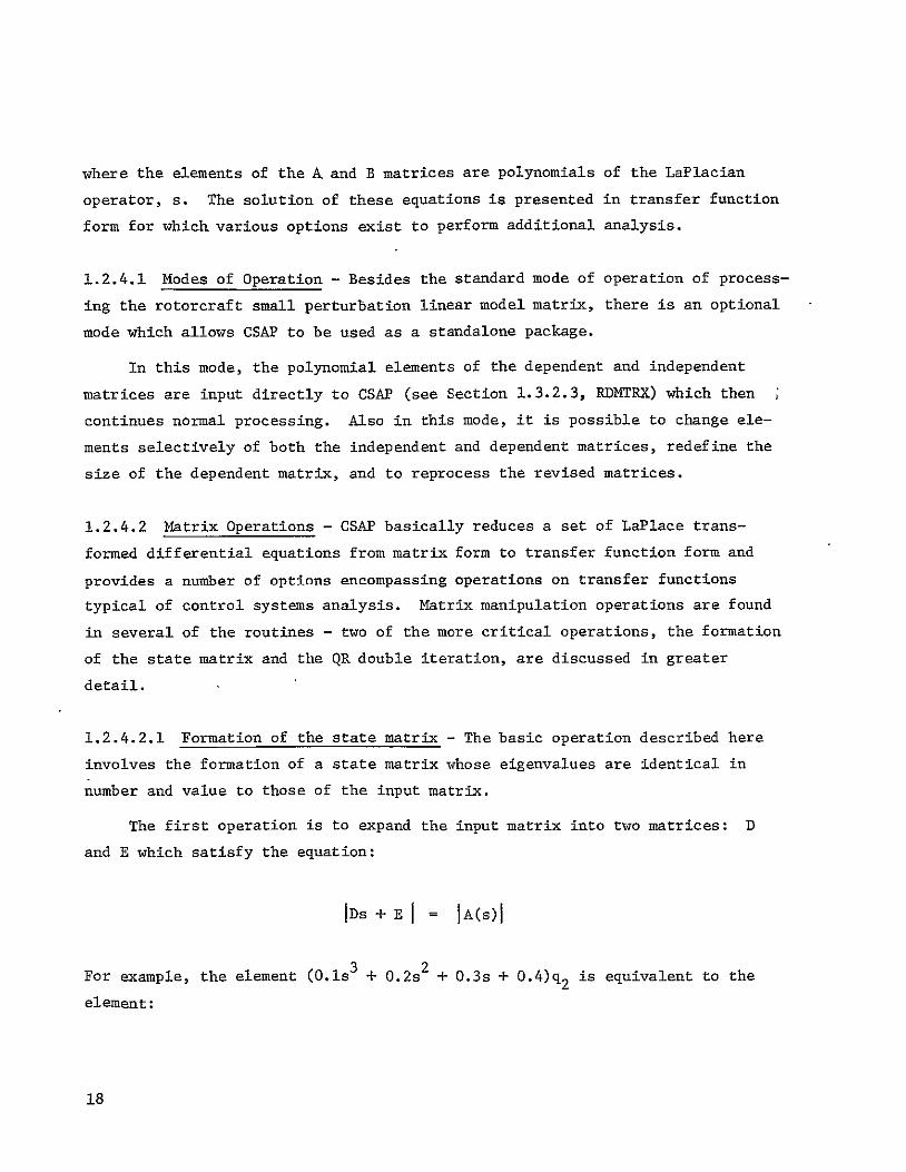
1.2.4.2.1 Formation of the state matrix - The basic operation described here

involves the formation of a state matrix whose eigenvalues are identical in

number and value to those of the input matrix.

The first operation is to expand the input matrix into two matrices: D

and E which satisfy the equation:

IDs + E I = IA(s)I

For example, the element (O.ls3 + 0.2s2 + 0.3s + 0.4)q2 is equivalent to the

element:

18

O.lsqN + 2 + 0.2sqN + i + 0.3sq 2 + 0.4q2

with the added equations:

s q2 - qN + 1 = 0

s qN+ 1 - qN + 2 = 0

the program keeps tab of the derivatives it has relabeled in the ITAB array.

At this point, some redundancy is possible in that the coefficient of sqi

could be placed either in the D matrix or the E matrix if that derivative has

been generated as a variable. If a choice exists, after the D and E matrices

are formed, the elements are all placed in the E matrix.

The next operation eliminates the off diagonal elements of the D matrix,

where possible. The row which contains the largest element of each successive

column is used for that column and a simple Gaussian elimination is used for

both that row and column. That row is also scaled such that the magnitude of

the pivot element is set to unity. The running product of these scale factors

(saved as DET) will be the determinant of the original D matrix and thus the

leading coefficient of the characteristic equation. I.e.,

IDs- El = IDIsn + .... -JEJ

In the general case, the off diagonal elements cannot all be eliminated,

i.e., IDD= 0. Three possibilities exist:

e For a null row in D, a nonzero element exists in E at the intersection

of a column which has not been pivoted.

19

For this case a Gaussian elimination is performed on the nonpivoted

column, DET is updated and that row and column are eliminated. For the

above example this would yield

* A second case exists where the pivot element of E is zero.

X 0 01S zxXx

For this case, the subject row is treated as an algebraic equation, i.e., = z q2 - y ql allowing the elimination of one of these variables. The

example would be:

-y/z 0 s x 0 X

0 000 0

After reducing in order:

Again the product DET is updated. At this point the program returns

to the point where we started the elimination of the off diagonal ele

ments of the D matrix.

20

a The third and last case covers the possibility of zero characteristic

equation (can be caused only by errors on the input - fewer equations

than variables). For this case the matrix may appear as:

1 s- x

0 0

The determinant of which is obviously zero. Control goes to the next

data case or numerator transfer function after an error message is

printed.

The state matrix is considered complete when its associated D matrix is

the identity matrix. An exact zero is used for all numerical tests on zero.

To avoid numerical problems in all the manipulations required to generate

the state matrix, a special function is used. Since most of the operations

are of the form A X - B, a function was designed to set the result to zero if

the product A X is the same as B disregarding the four least significant bits

of the mantissas.

The methods described here for the formation of the state matrix are used

for both the denominator and numerator functions. Cramer's rule is used to

form the matrix which yields numerator information.

1.2.4.2.2 QR double iteration - The following discussion concerning the QR

double iteration method used to find the eigenvalues of a real matrix is

excerpted from IBM's System/360 Scientific Subroutine Package - Programmer's

Manual, Reference 1.

1.2.4.2.3 Definition of the QR iteration - Let A be a real or complex non

singular matrix of order n. Then a decomposition of A exists of the form

A = QR

21

where Q is unitary and R is upper triangular. If the diagonal elements of R

are real and positive, Q is unique. Consider now the sequence of matrices

A (p ) defined recursively by

A(o) = A,

A(P) =QCP) R(P)

R( p ) A(P + 1) Q(P) p 0.

Note that A (p + 1) q(P)* A(p ) Q(P) for p 0; hence it follows that A(P)

is similar to A for all p.

Furthermore, if A satisfies certain conditions, it can be proved that A(p )

tends to an upper triangular matrix as p - w; thus the eigenvalues of A are

the diagonal elements of this limit matrix.

1.2.4.2.4 The double QR iteration - Let A be a diagonalizable real upper

Hessenberg matrix. Such a matrix must be expected to have complex conjugate

pairs of eigenvalues. If these pairs are the only eigenvalues of equal modulus,

it can be shown that they will appear as the latent roots of main submatrices

of order 2. In this case, if a shift is close to one of these roots, it will

be complex, and we will have to deal with complex matrices, although the initial

one is real. The use of the double QR iteration avoids this inconvenience.

Taking s(p + 1) = s(p ) , consider the transformation giving A(p + 2)

from A( p ) :

ACp + 2) = Q(p + i)* Q(P)* A(p) Q(p) Q(p + 1)

It can be proved that the product Q(P) Q(P + 1) derives from the QR de

(A(p ) (p ) I) (A(p ) (p composition of the matrix 1 = - s - s + 1) 1), which is

real.

It can be shown that only the first column m1 of M is necessary

2) from A(p ) , iffor determining the transformation which gives A(P +

they both have the Hessenberg form.

22

Practically, the first part of the double iteration consists of the

application of an initial transformation N A (p ) N where N is unitary and1 N1 whr 1 i ntr n

such that N1 ml ± Jim el. This leads to a matrix which no longer has

the Hessenberg form.

11

Thus, the remaining part of the iteration will involve the application of

(n - 1) successive transformations, which have the same form as the initial one

whose matrices N1 are such that the resulting matrix A (p + 2) has the Hessenberg

form.

This process can fail when a subdiagonal term of the given matrix is zero.

In this case, the matrix can be split, and the iteration is performed on the

lower main submatrix only.

1.2.4.3 Output Description - All matrix definition input data are printed.

Nondefined elements are assumed zero and are not printed. The dependent matrix

data are printed first and the independent matrix data are printed next. Each

element of the dependent and independent matrices are polynomial in the trans

form operator and are printed with the highest order coefficient first.

The characteristic equation in both factored and polynomial form is printed

with the denominator title. The polynomial is formed by the product:

N

P(s) = [ - s.)

The polynomial that is printed is the characteristic equation with the leading

coefficient divided out. This coefficient is printed.

Additional information such as time to one-half amplitude in seconds,

damping ratio, damped and natural frequencies (Hz) is supplied.

Eigenvectors are listed for each root with nonnegative imaginary part.

These vectors are solutions to the equation:

[A(s)] tvl = 0

23

where V is the vector that is listed and A is the input matrix. The special

case of multiple roots is not treated.

Output similar in form to that given for the characteristic equation is

given for each numerator requested with the exception of the eigenvectors.

For each numerator, K(s)/YLCs) so obtained, any one of several options may be

exercised:

• root locus

* frequency response

* power spectral density

* time history

See the individual output option routines for further discussion.

1.2.4.4 Data Storage - In order to conserve the storage requirements of the

control systems analysis package (CSAP), the input dependent and independent

matrices data are compressed into two arrays - IDATA and DATA.

IDATA is a two-dimensional array, whose rows represent code, row, column,

and order information defining the matrix polynomial element. The DATA array

contains the values of the coefficients of each matrix element.

An example is given to illustrate the compressed data storage technique

used:

e.g.,

element stored

Code: IDATA(l,l) = 0 DATA(l) = 1

Row: IDATA(2,1) = 2 DATA(2) = -5

Column: IDATA(3,1) = 1 DATA(3) = 4

Order: IDATA(4,l) = 2

The first element stored defines the (2,1) element of the dependent matrix

as:

24

s - 5s + 4

element stored

Code: IDATA(l,2) = 1 DATA(4) = .5

Row: IDATA(2,2) = 1

Column: IDATA(3,2) = 1

Order: IDATA(4,2) = 0

The second element stored is the (1,1) element of the independent matrix

and has the value of:

0.5

Note that the code (i.e., row 1) found in the IDATA array translates as

follows:

* 0 - element belongs to the dependent matrix

o 1 - element belongs to the independent matrix

* 2 - end of matrix definition data

When selectively redefining matrix elements (subroutine NWMTRX), the origi

nal element definition information in the IDATA array is effectively nulled by

setting the row definition to zero. The new definition is then added after the

last definition of both the IDATA and DATA arrays. This technique is used

because the order of the revised polynomial is not necessarily the same as the

original and simply storing the new over the old would cause subsequent

erroneous retrieval of the data.

1.3 Subroutines

The following subsections treat each of the subprograms in the linear

model package. The function of each routine, call arguments and programming

notes are given. The level of detail is intended to be sufficient to enable

one to work with the coding to troubleshoot or make modifications.

25

1.3.1 CPUNCH

The function of this routine is to punch the dependent and independent

matrices in the order specified form (see Section 1.3.25 RDMTRX).

Routine access:

Call CPUNCH (DATA,MD,IDATA,MI)

Input:

DATA - Compressed matrices value vector

MD - Dimension of DATA vector

IDATA - Compressed matrices definiton array

MI - Dimension of IDATA array

Output:

Punched cards

Notes:

" Logical unit 7 is assumed to be the card punch unit

" Currently, only second-order polynomials or less are punched.

(This is due to the format statement which can be easily

changed.)

1.3.2 DERIVE

Subroutine DERIVE computes the aerodynamic partial derivatives for

the rotorcraft main rotor, tail rotor, and fixed surfaces. The main

rotor derivatives are formed in array DERIV. This array is made from the

basic derivatives, which also use DERIV, and inflow compounded partials

26

from the basic derivatives, LAMDRV. The fixed surface partials are computed

in the array FIXED. Tail rotor and some fixed surface partials are individ

ually named.

The FIXED array elements are developed in section 3.1.3 of Volume I. Tail

rotor terms are given in section 3.1.4. Inflow derivatives and the method of

forming the inflow array LAMDRV are in section 3.3.2, and the derivative com

pounding scheme is in section 3.3.3 of Volume 1. The main rotor partials are

given in sections 3.3.3.1 through 3.3.3.4, and are used to form the DERIV array.

Routine access:

Information is transmitted via common statements.

Input:

/ABC/ lCommon; Input physical constants.

/PASSTR/ 'Common; Trim and preliminary calculations.

/TRIMAC/ Common; Trim data and physical inputs.

/PASSIN/ Common; Inflow partial derivatives from INFLOW program.

Output:

/PASSDE/ Common; Contains DERIV and FIXED arrays.

/TRIMAC/ Common; Contains vertical tail and tail rotor partial

derivatives.

Notes

e Array arrangement scheme is given in Volume 3. under Section 3.5,

Output Description.

1.3.3 DPQFB

The purpose of the routine DPQFB is to find an approximation of the form

Q(x) = Ql + Q2 x + x2 to a quadratic factor of a given polynominal, P(x),

with real coefficients. Bairstow iteration is used. See Reference 1.

27

Routine access:

CALL DPQFB (C, IC, Q, LIM, IER)

Inputs:

C - Vector containing the coefficients of P(x), with C(1) being

the constant term.

IC - Order of polynominal

Q - Q(1) and Q(2) are initial trials for Q, and Q2 "

LIM - Limit number of iterations

Outputs:

Q - Q(1) and Q(2) contain the refined coefficients of Q1 and Q2 "

Q(3) and Q(4) are the coefficients of the remainder A + Bx

of the quotient P(x)/Q(x).

IER - Error flag:

= 0 no error

= 1 no convergence within allowed iteration limit

= -1 polynomial P(x) is constant or undefined

= -2 polynomial P(x) is of degree 1

= -3 no further refinement of the approximate quadratic

factors is feasible, initial guess is not close enough.

Notes:

" No subroutines are called.

* Checks on .overflow have been removed from the CDC version. Subroutine

OVERFL is an IBM service routine

a Variables EPS and EPSI are used in the accuracy tests. Values are set

to be compatible with IBM DOUBLE PRECISION. These coefficients may

be set to achieve the desired accuracy.

28

1.3.4 DPRBM

Subroutine DPRBM calculates the roots of a given polynomial with real

coefficients. The roots are computed by successive quadratic factorization

using the Bairstow iteration method via calls to routine DPQFB.

Routine access:

CALL DPRBM (C, IC, RR, RC, POL, IR, IER)

Inputs:

C - Vector containing the coefficients of the given polynomial.

The coefficients are ordered from low to high, and on return

they are divided by the last non zero term.

IC - Number of coefficients in vector C.

Outputs:

RR - Vector containing real part of the roots.

RC - Vector containing complex parts of the roots.

POL - Vector containing coefficients of the polynomial using the

calculated roots. The coefficients are ordered from low to

high.

IR - Number of calculated roots.

IER - Error flag:

= 0 no error

= 1 poor convergence of subroutine DPQFB

= 2 polynomial is degenerate

= 3 subroutine bypassed due to zero 'divide or unsatisfactory

accuracy

= -1 poor accuracy of calculated roots; less than three cor

rect significant digits.

29

Notes:

* Subroutine calls: DPQFB

* Checks on overflow have been removed from the CDC version.. Subroutine

OVERFL is an IBM service routine.

" Vectors are arranged so that the constant term is in position 1.

" Variable EPS is used in accuracy tests. Value currently compatible

with IBM DOUBLE PRECISION, but can be set for desired accuracy.

1.3.5 EIGVAL

,Subprogram EIGVAL is an executive subroutine which finds and prints the

eigenvalues of a state matrix. Routine HSBGNM converts the state matrix into

Hessenberg form which is then passed to the QR routine which computes the

eigenvalues of the input matrix. Using the computed roots, subroutine PLYFRM

forms a polynomial. The roots are then printed by routine PRINTR.

Routine access:

CALL EIGVAL (IB, D, JJ, ITITLE, DET, RR, RI, PN)

Inputs:

D - Matrix whose eigenvalues are to be found

IB - Dimension of D

JJ - Order of the input matrix

DET - Determinent of the input matrix

ITITLE - 80 byte title associated with the input matrix

Outputs:

RR - Vector containing real parts of the roots

RI - Vector containing imaginary parts of the roots

PN - Vector containing coefficients of the polynomial ordered low

to high.

30

Notes:

* Subroutine calls:

HSBGNM, QR, PLYFRM, PRINTR

a Ordered low to high means the constant term is in P(1).

1.3.6 EIGVEC

The original dependent variable matrix is utilized to determine eigen

vectors. Thus the vectors which are printed represent the relationships of

the original problem variable. (not necessarily the state variables) for each

mode. This is accomplished by evaluating the dependent variable matrix at

each root s = si:

[A(s)] [A +iATi]

The two matrices Ai, AIi are then passed to the subroutine VECTOR which

(usually) returns the non trivial solution V to the equation

[AR+jA1I] {VR +ijVT} = 0

This process is repeated for each root with zero or positive imaginary

part.

Routine access:

CALL EIGVEC (IB, D, E, ND, DATA, MI, IDATA, RR, RJ, NRUT, N)

Inputs:

DATA, IDATA - matrices containing compressed form of both the depen

dent and independent matrices

MD, MI - dimension of DATA and IDATA arrays

31

RR, RI - Vectors containing the real and complex parts of the

roots of the dependent matrix

NRUT - number of roots

N - number of dependent 'variables

D, E - work arrays used to compute and print the eigenvectors

IB - dimension of D and E

Outputs:

Print only

Notes:

* Subroutine calls: VECTOR

* The conjugate root (i.e., negative imaginary part) will produce the

conjugate vector. (i.e., VR - jVI) and therefore is not computed.

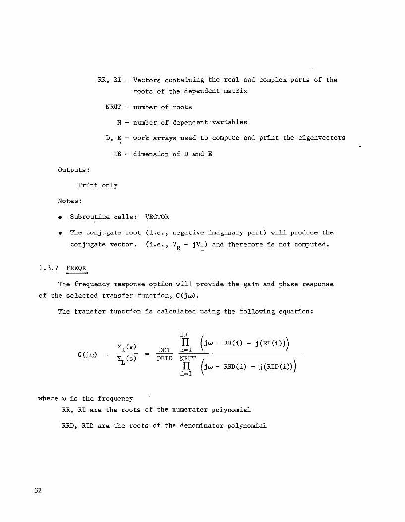
1.3.7 FREQR

The frequency response option will provide the gain and phase response

of the selected transfer function, G(jc).

The transfer function is calculated using the following equation:

Jj

k~s DE (.jco- RR(i) - (RI (i))) TQ K(s) DET i=l

G YL (S) DETD NRUT E(c - j(RID(i)))Oi I -RRD(i)

where w is the frequency

RR, RI are the roots of the numerator polynomial

RRD, RID are the roots of the denominator polynomial

32

The frequency is incremented in geometric progression to yield equal

spacing on the typical Bode log frequency plot.

Gain and phase information are printed for each frequency and saved for

later plotting (optional). Note that a full page of print is generated before

a check is made on the maximum frequency.

Routine access:

CALL FREQR (IPLOT, DAT)

Inputs:

IPLOT - Vector containing plot control data

DAT - Vector containing frequency response control data

/TITLE/ - Common; denominator and numerator titles

/REALA/ - Common; Vectors containing the real and imaginary parts

of the roots of the denominator and numerator

/PLOTC/ - Common; plotting information

/OPTION/ - Common; miscellaneous information passed from MAIN

routine.

Outputs:

Print only

Notes:

* Subroutine calls: PLXDIV, YPLOT

* A full page of print contains information about 72 points printed

in two columns; 36 print lines per page.

33

1.3.8 GELG

GELG solves the set of linear equations AX B by Gaussian elimination.

See Reference 1 for a complete description.

Routine access:

Call GELG (B,A,M,N,EPSIER)

Input:

B - Input matrix of dimension M by N containing right-hand sides

of the equation AX = B. (destroyed)

A - Input matrix of dimension M by M containing the

matrix of the equation AX = B. (destroyed)

M - Number of equations in the system (order of A and number of

rows in B).

N - Number of right-hand sides (vectors).

EPS - Input constant used as relative tolerance for test on loss

of significance.

Outputs:

B - The m by m solution.

IER - RESULTING ERROR PARAMETER CODED AS FOLLOWS

IER=O - NO ERROR.

IER=-l - NO RESULT BECAUSE OF M LESS THAN 1 OR PIVOT

ELEMENT AT ANY ELIMINATION STEP EQUAL TO 0.

IER=K - WARNING DUE TO POSSIBLE LOSS OF SIGNIFICANCE

INDICATED AT ELIMINATION STEP K+1, WHERE PIVOT

ELEMENT WAS LESS THAN OR EQUAL TO THE INTERNAL

TOLERANCE EPS TIMES ABSOLUTELY GREATEST ELEMENT

OF MATRIX A.

Notes:

a EPS between 1014 and 1616 is suggested by 64-bit word

computations.

34

1.3.9 HSBGNM

The purpose of this routine is to convert an input state matrix into

Hessenberg form and to compute a scaled Euclidean norm.

The scaled Euclidean norm is computed using the following equation.

2 I

=(X)N2

i=l j=l

The real matrix A is reduced by a similarity transformation to Hessenberg

form. Each row, starting from the last one, is reduced by applying a suit

able right elimination matrix and similarity is achieved by also applying

the left inverse transformation. The end result is an upper almost

triangular matrix whose eigenvalues are the same as the original input

matrix.

Routine access:

CALL HSBGNM (A, IORD, MAXS, ENORM, N)

Inputs:

A - matrix to be converted

IORD - order of A

MAXS - dimension of input matrix and work vector, N

N - work vector

Output:

A - Hessenberg form of original input matrix

ENORM - Scaled Euclidean norm

35

Notes:

a The Euclidean norm is scaled by the formula:

-N BITS= qA + 2ENORM

where NBITS is the number of significant bits used. The value of

ENORM is used to find computational zero.

1.3.10 INFLOW

INFLOW calculates the steady state, sine and cosine components of the

main rotor induced velocity as a function of the degrees of freedom. An

implicit relation is formed for the three variables. The resulting array

is inverted using GELG to find the explicit partial derivatives. The inflow

array is given in Section 3.3.2 of Volume I.

Routine access:

The routine information is processed via COMMON statements.

Input:

/ABC/ Common; Input data physical constants

/PASSTR/ Common; Calculations from TRIM program.

/TRIMAC/ Common; Input data and TRIM calculations.

Output:

/PASSIN/ Common; LAMDRV array of inflow partials.

1.3.11 MAIN

This routine controls the linear model sequence of computations as illus

trated in Figure 1-i. First, a call is made to PDATE which returns the current

day's date. Then information about the matrices is read and depending upon

36

the specified mode of operation, control is passed to either routine MODEL

or RDITRX which return the independent and dependent matrices in compressed

form. Before these matrices are analyzed, their nonzero values are printed

(subroutine PRINT).

Next, routine STMTRX forms the state matrix and then the denominator

title is read and the eigenvalues and eigenvectors are computed (subroutines

EIGVAL and EIGVEC).

After reading the numerator title and determining that output options

are desired, control information about the output options is read. The

numerator state matrix is formed (routine STMTRX) and it's roots are com

puted (subroutine EIGVAL). Control is then passed to the appropriate

output option routine (subroutines ROOT, FREQR, TIMEH or POWER). This loop

repeats until all the output options indicated have been completed.

If changes to the original matrices are desired, routine NWMTRX reads

the selected matrices elements to be changed and then the revised matrices

are printed (subroutine PRINT). The program then repeats from the point

where the original state matrix is computed.

When-the particular case is done, the program checks if another con

figuration is to be run. If another case follows, control cycles back to

the point where the input data is read.

1.3.12 MATRIX

The routine MATRIX uses the coefficients from TRIM to establish the

linear model in matrix form. MATRIX calls INFLOW and DERIV in order to

compute the required aerodynamic partial derivatives. The matrix elements

are calculated as four arrays. MTRXA contains the second order terms,

MTRXB has the first order terms, and MTRXB is the array of constants. The

INDEP array contains the forcing functions. The matrix model is given in

Figure 4-1 of Volume I.

37

Routine access:

This routine handles information via COMMON statements.

Input:

/PASSDE/ Common; Aerodynamic derivatives.

/ABC/ Common; Input physical data.

/TRIMAC/ Common: Trim rates and aerodynamic derivatives.

Output:

/PASSMX/ Common; Contains the MTRXA, MTRXB, MTRXC and INDEP

matrices.

Notes:

* This routine calls INFLOW and DERIVE.

1.3..j MODEL

The program MODEL is an executive routine that calls the subroutines

necessary to create and assemble the linear model matrix, and submit it

for analysis processing. There are no direct input or output functions.

The routines READIN, TRIM, MATRIX and PKDATA are called in order.

1.3.:4 NWMTRX

NWMTRX allows changes to be made to either a model defined by MATRIX

or direct input by the user.

The revised definition for the original dependent or independent matrix

element is read. Then, if the original matrix element definition exists,

it is nulled. The revised definition is added to the next free location

in the compressed matrices. This process is repeated until the revisions

are exhausted.

If a change to the dependent matrix size is indicated, then this change

is made.

38

Routine access:

CALL NWMTRX (LI, LX, INPUT, IDATA, MI, DATA, MD, N)-

Input:

INPUT - Input method flag

IDATA, DATA - Matrices containing compressed form of both the

original dependent and independent matrices

MI, MD - Dimensions of the IDATA and DATA arrays

LI - Pointer to the next available location in the IDATA

array

LX - Pointer to the last used location in the DATA array

N - Number of dependent variables

Notes:

* This routine has no output pther than to change the model matrix.

1.3.15 PDATE

Routine PDATE is a dummy date routine which is replaced by the particular

installation's own date routine. The calling routine expects a one word,

eight character literal to be returned.

Routine access:

CALL PDATE (NDATE)

Output:

MM-DD-YY, Month, day, year

Notes:

a The argument NDATE is typed DOUBLE PRECISION for the IBM version and

REAL for CDC and is left-justified.

39

1.3.16 PKDATA

Routine PKDATA packs the general A, B, and C matrices calculated in

subroutine MATRIX into the form required by the matrix analysis section of

this program.

Routine access:

CALL PKDATA (IDATA, MI, DATA, MD, LX, LI, N, INV, IER)

Input:

MI - Column dimension of IDATA array


N - Number at dependent variables

INV - Number of independent variables

/PASSMX/ - Common; general A, B, C and INDEP matrices

Output:

IDATA - Compressed dependent and independent matrices definition

data array

DATA - Compressed dependent and independent matrices coefficient

data vector

LX - Pointer to the last used location in the DATA vector

LI - Pointer to the next available location in the IDATA vector

IER - Error flag

= 1 number of defined matrix elements exceeds dimension

of IDATA array

= 2 number of defined matrix elements exceeds dimension

of DATA vector

40

1.3.17 PLXDIV

The function of this routine is to perform the complex division:

u + jv =, (A + jB) / (C + jD)

The input values A, B, C and D are first normalized such that MAX (C, D)

is unity. The solution is then obtained from:

u (A' * C' + B' * D') / (A' * A' + B' * B')

v (B' * C' - A' * D') / (A' * A' + B' * B')

The original A, B, C and D are not destroyed.

Routine access:

CALL PLXDIV (A, B, C, D, U, V)

Input:

A, B - Complex numerator variable

C, D - Complex denominator variable

Output:

U, V - Complex quotient of division operation

1.3.18 PLYFRM

The subroutine PLYFRM forms a polynomial from its roots. I.e.,

NRUT

P(s) = J (s-s i) i= 1

where the s. are the real or complex roots which define the system. TheI

method used is a straight forward multiplication which will handle the

41

N=0 case. Conjugate roots are assumed. The constant term is in the P(0)

slot and the leading coefficient (1.0) is placed in P(N).

Routine access:

CALL PLYFRM (NRUT, RR, RI, P)

Inputs:

NRUT - Number of roots

RR -Vector containing real parts of the roots

RI - Vector containing imaginary parts of the roots

Outputs:

P -Vector containing the coefficients of the computed polynomial

ordered low to high

Notes:

" Conjugate roots are assumed

* The N=0 case is handled

* Ordered low to high means the constant term is in the P(1) location.

1.3.19 POLRT

Subprogram POLRT computes the roots of a polynomial with real coef

ficients using the Newton-Raphson successive approximation iterative tech

nique. See Reference 1.

Routine access:

CALL POLRT (XCOF, COY, M, ROOTR, ROOTI, IER)

Inputs:

XCOF - Vector containing the coefficients of the polynomial

ordered low to high

COF - Working vector of length M + I

M - Order of the polynomial.

42

Outputs:

ROOTR - Vector containing real parts of the roots

ROOTI - Vector containing imaginary parts of the roots

IER - Error flag

= 0 no error

= I order of polynomial less than one

= 2 order of polynomial too big (i.e., >36)

= 3 unable to find roots

Notes:

" The program contains a section of code to test the accuracy of

each root and print a warning of insufficient accuracy.

* The accuracy test numbers are compatible with IBM DOUBLE PRECISION.

These values can be changed to achieve the desired accuracy.

1.3.20 POWER

This routine forms a power spectral density solution to a selected

transfer function. This operation is not part of the usual linear model

procedures, but is included here to fully describe the analysis package

routines.

Subroutine POWER computes the turbulence power spectral density and

the density integral of the transfer function, XK(S)/YL(S). The power

spectral density is calculated from the equation:

2PSD(O) = G(jw) 2L 1 + 8/3(l.339wL/v)2 v (I + (l.339wL/v)2 ) 11/6

43

where

G(j) = XK(J)/YL(0C)

w is the frequency

L is the characteristic length

v is the velocity

Note that

1 eln(x)/61 11/6 2 x x

which is used to simplify to previous equation.

Then the density integral at each frequency is calculated using the

equations

PH i = PSD (i) ( - 1)(1 - Y( _)1i PHI(w) 2 211 + PHI (o1 )

where Awis the frequency increment PHI (wi) = 0

Frequency, the magnitude of the transfer function (i.e., JG(jw)12),

the power spectral density and density integral information are printed.

The frequency and PSD, are also saved for later plotting (optional).

Routine access:

CALL POWER (DAT, IPLOT)

Input:

DAT - Vector containing control data for this option

IPLOT - Vector containing plot control data

/TITLE/ - Common; denominator and numerator titles

44

/REALA/ - Common; vectors containing the real and imaginary

parts of the roots of the numerator and denominator

/OPTION/ - Common; miscellaneous information passed from MAIN

routine


Outputs:

Print only

Notes:

a' Subroutines PLXDIV and ZPLOT are called.

e The frequency is incremented in geometric progression to yield

equal- spacing on logarithmic frequency scales.

o Note that for a unity transfer function (i.e., G(jQw) = 1), the integral will approachunity as wmin ' 0 and w -m W. The

mm max

resulting power spectral density will be that of the isotropic

turbulence model with unity standard deviation.

1.3.21 PRINT

The function of this routine is to print the dependent and independent

matrices.

The dependent matrix is printed beginning with row 1. All the poly

nomial elements in row 1 are collected, sorted in column order and printed.

This process is repeated for all the rows of the dependent matrix.

The independent matrix is then printed using the same method.

Routine access:

CALL PRINT (D, IB, DATA, MD, IDATA, MI, N)

45

Input:

D - Working array

IB - Dimension of D

DATA, IDATA - Matrices containing the compressed form of both the

independent and dependent matrices

MD, MI - Dimensions of the DATA and IDATA arrays


Output:

Print only

Notes:

* Only the defined (i.e., non-zero) input are printed

e For each row, the number of lines of print per row is determined

by the highest order polynomial in that row.

* The constant term appears last.

1.3.22 PRINTR

This routine is used to print polynomial, root and stability information.

The routine recognizes three possible cases where the information printed

is dependent upon the imaginary part of the root. If the imaginary part of

the root is:

1) negative - only polynomial and root information is printed

2) zero - polynomial, root and time to half amplitude information

is printed.

3) positive - polynomial, root and all stability information is printed.

46

The formulas used to compute stability information are:

Time to half amplitude = -. 69314718/RR

Damping ratio = -RR/WN

Damped frequency (D) = RI/6.2831853

Damped frequency (N) = 1N/6.2831853

where

2 2 1/22 )(RR

2 + RI =WN

and each root is located at RR + j RI.

Routine access:

CALL PRINTR (J, RR, RI, P)

Input:

J - Number of roots

RR, RI - Vectors containing real and imaginary parts of the roots

P - Vector containing coefficients of the polynomial formed

using the roots. Ordered low to high.

Output:

Print only.

1.3.23 PROD

Subroutine PROD performs the calculation:

PROD =A - B * C

47

If the difference between A and B * C is equal to or greater than the

fifth least significant bit of the mantissa of A, otherwise PROD = 0.0.

Routine access:

Function subroutine; X = PROD (A, B, C)

Input:

A, B, C - Input variables

Output:

Value of the computation A - BC

1.3.24 QR

Subroutine QR calculates the eigenvalues of the input Hessenberg

matrix using the QR double iteration process. See Section 1.2.4.2.2.

Routine access:

CALL QR (A, N, MAXS, E, RR, RI, ITER)

Input:

A - Input matrix in Hessenberg form.

N - Order of A

MAXS - Dimension of A and ITER

E - Scaled Euclidean norm

ITER - Work vector

Output:

RR - Vector containing real parts of the eigenvalues

RI - Vector containing imaginary parts of the eigenvalues

48

Notes:

" No subroutines are required.

" At each iteration, the latent roots X I and X 2 of the lower main

submatrix of order 2 are computed. The following' situations can

occur:

a) A (N, N - 1) 0. A (N, N) is an eigenvalue. The order is

reduced by one

b) A (N - 1, N - 2) = 0. and X 2 are eigenvalues of the originalX I

matrix. The order is reduced by two.

1.3.25 RDNTRX

An optional mode of the linear model allows the user to use the pro

gram as simply a control systems analysis tool (CSAP). In this mode the

dependent and independent matrices are directly inputted to the program

in one of two forms:

1) K, I, J, M, DAT FORMAT (412,6FI0.0)

2) K, I, J, DAT FORMAT (312,3F10.0)

where

K = 0 dependent matrix element

= 1 independent matrix element

= 2 end of matrix data

49

I row of matrix element

J column of matrix element

M order of polynomial

DAT coefficients of polynomial

for method #1, DAT = A , A .... , A

#2, DAT = A2, Al, A 0

This input data is stored in compressed form. See Section 1.2.4.4.

Routine access:

CALL RDMTRX (IDATA, MI, DATA, MD, LX, LI, INPUT)

Input:

MI - Dimension of IDATA array


INPUT - Flag indicating input format

Output:

IDATA - Compressed matrices definition array

DATA - Compressed matrices value vector

LI - Pointer to next available location in IDATA array

LX - Pointer to last used location in DATA array

Operation of the program in this direct mode is discussed in Sec

tions 3.2 and 3.3 of Volume III.

50

1.3.26 READIN

The routine reads the linear model case definition data, and prints an

echo of this data with group titles.

Routine access:

CALL READIN (0)

Inpt:

Input data cards numbers 2 through 19.

Output:

0 - Omega frequency used in plotting the time history option

/ABC/ - Common; input case configuration data.

1.3.27 ROOT

The root locus option, via subroutine ROOT, finds the roots of the

system:

1 + GAIN (i) * Xk(s)/YL (s) = 0

Replacing the numerator and denominator (K and YL) of the transfer

function by their respective polynomial form (i.e. PN and PD) and multiplying

by the denominator, the following equation is formed which is the actual equa

tion whose roots are found:

F(s) = PD (s) + k * DET/DET * PN (s)

for each value of k (GAIN).

The numerator polynomial is input to this subroutine which calls PLYFRM

to form the denominator polynomial. Subroutine RTPOLY is then used to calcu

late the roots which are printed by the PRINTR routine.

51

The denominator roots and the roots of the above equation are saved in a

data array for plotting. Also, the largest and smallest roots of the denomi

nator, numerator and the above equation are found for plotting purposes.

Routine access:

CALL ROOT (MI, PN, DAT, IPLOT, ZEROX, ZEROY)

Input:

NI - Order of ZEROX and ZEROY vectors

PN - Numerator polynomial

DAT - Root locus control data vector

IPLOT - Plotting control data vector

ZEROX - Vector containing real parts of the numerator roots

ZEROY - Vector containing imaginary parts of the numerator roots.

/REALA/ - Common; real and imaginary parts of the roots of the

denominator and numerator.

/TITLE/ - Common; numerator and denominator titles


/OPTION/ - Common; miscellaneous information passed from MAIN routine.

Output:

Print only.

Notes:

* Subroutines required. PLYFRM, PRINTR, RTPOLY, XMAX, XMIN, ZPLOT

* Plotting capability has not been implemented on the CDC version.

1.3.28 RTEST

This routine creates the polynomial from the trial roots.

52

The polynomial P(s) is evaluated at s = s.1 using the following equation:

n-i

P(s) = a0 + E aksk

s+s. k=l

Routine access:

CALL RTEST (COEF, RE, N, IMAG, FC, FD)

'Input:

COEF - Vector containing the coefficients of the polynomial

ordered high to low.

RE - Real part of s = s.1

IMAG - Imaginary part of s = s.1

Output:

FC - Vector containing real part of evaluated polynomial

FD - Vector containing imaginary part of evaluated polynomial.

1.3.29 RTPOLY

Subroutine RTPOLY is an executive routine for finding the roots of a

given polynomial. Three attempts to compute the roots are made.

Control is first passed to routine DPRBM which attempts to calculate the

roots by successive quadratic factorization using the Bairstow iteration

method.

If subprogram DPRBM is unable to find the roots of the polynomial, then

an initial guess is made on the roots to be found. Control then passes to

subroutine POLRT which employs the Newton-Raphson iterative method to

compute the roots of the polynomial.

If the first pass through POLRT fails, another initial guess is made and'

subprogram POLRT is again invoked. If this third attempt to find the roots

53

of the polynomial fails, an error message is printed and control returns to

the calling routine.

Both the Bairstow and the Newton-Raphson iterative techniques are used

in order to ensure that the roots will almost always be found. This is due

to the fact that the class of polynomials for which one method fails to con

verge is not the same as the other.

Routine access:

CALL RTPOLY (N, C, L, F, RR, RC, POL)

Input:

N - Order of the polynomial

C - Coefficients of the polynomial ordered high to low

F - Dummy argument

Output:

RR - Vector containing the real parts of the roots.

RI - Vector containing the imaginary parts of the roots.

POL - Vector containing the polynomial coefficients using the

calculated roots.

L - Error flag.

Notes:

* Subroutines required: DPRBM, PORT

1.3.30 STMTRX

The basic function performed by routine STMTRX is to form a state matrix

whose eigenvalues are identical in number and value to those of the input

matrix. The method used is explained in Section 1.2.4.2.1 Formation of the

state matrix.

Routine access:

CALL STMTRX (MD, MI, IDATA, DATA, JD, JN, JB, N, D, E, DET, J, IER)

54

Input:

MD, MI - Dimensions of DATA and IDATA arrays

IDATA, DATA - Arrays containing compressed matrices data

JD - Dependent variable column number j used for transfer function

computations

JN - Independent variable column number i used for transfer func

tion computations

IB - Size of D and E arrays


E - Work array

Output:

D - State matrix

DLT - Determinant of input matrix

J - Order of state matrix

IER - Error flag

Notes:

o Subroutine calls: PROD

1.3.31 TIMEH

The time history option computes a step response time history for a

specified transfer function. The equation:

DET -1 1PN (s)f(t) DETD 1 D

Where L is the inverse LaPlace transformation

55.

is solved by integration where the integration formula used is the fourth

order Taylor series expansion:

x(t + T) = x (t) k=0

This formula was chosen to take advantage of the fact that the derivatives of

each state variable are available at each point in time when the polynomial

form is utilized. The conceptual form is given in Figure 1-2.

Note that the derivatives of each state variable, x are available. The

derivatives of the lead integrator are found from the equation:

N-1

t) - = "-PD (i) * x(i + k - 1)

i=l

where STEP * DET/DETD is added for k=l to account for the step input-magnitude.

Values for position, rate and acceleration as a function of time are

printed and saved for later plotting (optional). An integration interval of

approximately .2/R is recommended where R is the distance in the S plane

from the origin to the largest denominator root. Note that in order to make,

the print time (TP) a near integer multiple of the integration interval (DT),

the following adjustment is made:

S(1 + 10- 6) *TPTP/STEPI

where STEPI is the integration step.

Routine access:

CALL TIMEH(PN, DAT, IPLOT, 0)

56

SPN (N-1)

XN-1 XN-2 Xo I IF (STEP DE L .... Prio (0)OTPT

INPUT) DETD

PD (N-1) ]

Figure 1-2. Time History Integration Format

57

Input:

PN - Vector containing coefficients of the numerator polynomial

DAT - Time history control data

IPLOT - Plotting control data

0 - Frequency used for scaling purposes

/TITLE/ - Common; numerator and denominator titles

/REALA/ - Common; numerator and denominator roots

/PLOTC/ - Plotting information

/OPTION/ - Miscellaneous information passed from MAIN routine

Output:

Print and plot only.

Notes:

* Plotting capability has not been implemented on the CDC version.

* Subroutine calls: PLYFRM, XPLOT

1.3.32 TRIM

The routine TRIM establishes a free flight force and moment equilibrium

from the rotorcraft defined by the input data. Angle of attack is iterated

to null the longitudinal force summation. Collective is used to null the

vertical force sum. The tail rotor thrust is set to balance the main rotor

torque. The main rotor inflow velocity is calculated as a convergence loop

within the vertical and longitudinal force balance loops. The balance equations

and coefficients are given in section 3.9 of Volume I.

Routine access:

CALL TRIM (IER)

Input and output information is handled by COMMON statements and

diagnostic printouts except for error indicator.

58

Input:

/ABC/ Common; This is the input physical constants.

Output:

/PASSTR/ Common; The trim constants calculated and frequently

used coefficient groupings.

/TRIMAC/ Common; Partially composed of TRIM computation outputs.

Trim conditions and coefficient groupings are printed by this

routine.

IER = Error flag:

= 0 no trim errors

= 1 convergence failure

Notes:

e The inflow iteration uses a weighted average of new and old trials

to achieve convergence. This weighting is internally scheduled

versus speed to optimize to convergence process for rotorcraft data

sets tried so far. The weighting coefficient mix or speed scheduling

may have to be altered if plus-minus iteration cycle problems develop.

1.3.33 VECTOR

The function of the VECTOR routine is to accept the complex matrix A

whose determinant is supposedly null and produce the complex vector V which

represents the solution to the equation:

[A] V = 0

The method used is to reduce A to a diagonal matrix through Gaussian elimina

tion and back-solve the column whose (n, n) term is zero for the vector.

The A matrix is destroyed and the vector is left in the JV column where JV

is an integer passed in the calling sequence.

59

Note that a zero is defined to be:

10-8 *Z JAR (I,J)j + JAI (I,J)I)/N

-8 -NBITS/2 -for all zero tests. The factor 10 approximates 2 . Where NBITS is

the mantissa length (48 for CDC 7600).

Subroutine access:

CALL VECTOR (IB, AR, Al, JV, N)

Inputs:

IB - Dimensions of AR, AI

AR - Work array; on input, contains real parts of input matrix

AI - Work array; on input, contains imaginary parts of input

matrix.

N - Order of input matrix

Output:

AR - Work array; on output, contains real part of solution

vector

AI - Work array; on output, contains imaginary part of solution

vector

JV - Column of AR, AI matrix which contains solution vector

Notes:

* Subroutine calls: PLXDIV

1.3.34 XHAX

The purpose of the XMAX function is to return the maximum value of the

input real array of length N.

Routine access:

Function BMAX = XMAX (A, N)

60

Input:

A - Real array

N - Size of A

Output:

XMAX - Maximum value of the input matrix

1.3.35 XMIN

The purpose of the XMIN function is to return the minimum value of the

input real array of length N.

Routine access:

Function BMIN = XHIN (A, N)

Input:

A - Real array

N - Size of A

Output:

XMIN - Minimum value of the input matrix

1.3.36 XPLOT

Subroutine XPLOT is the dummy plotting routine used by the time history

option (subprogram TIMEH).

Routine access:

CALL XPLOT

Notes:

* An active plotting routine can be constructed using the arguments

listed in the original call to this routine, the labeled cotnon

/PLOTC/ and knowledge of the installation's plot routines.

61

1.3.37 YPLOT

Subroutine YPLOT is the dummy plotting routine used by the frequency

response option (subprogram FREQR).

Routine access:

CALL YPLOT

Notes:

* An active plotting routine can be constructed using the arguments

listed in the original call to this routine, the labeled common

/PLOTC/ and knowledge of the installation's plot routines.

1.3.38 ZPLOT

Subroutine ZPLOT is the dummy plotting routine called by the power

spectral density and root locus options (subprograms POWER and ROOT).

Routine access:

CALL ZPLOT

Notes:

* An active routine can be developed using the data array PDATA, the

labeled common /PLOTC/ and the plotting routines of the particular

installation.

62

SECTION 2

COMMON/SUBROUTINE DIRECTORY

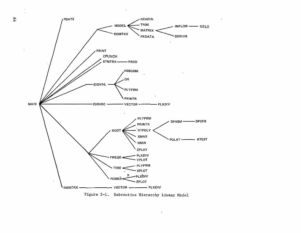
Figure 2-1 and Tables 2-1 and 2-2 are presented here as aids to under

standing the hierarchical structure of the linear model programming,. Fig

ure 2-i shows the calling sequence, or tree, of the package routines.

Table 2-1 lists each subroutine and the routines which it calls. The

called routines have a level number associated with them which indicate

whether the called routine in turn calls any other routines. A zero shows

no further 'alls, a one shows one additional sub level, etc.

Table 2-2 lists each COMMON block and the routines in which they are

used. All COMMON blocks are labeled.

63

4 PDATE

MODEL <

RDMTRX

READIN

TRIM N MATRIX

\PKDATA

INFLOWIELG

DERIVE

GELG

PRINT

CPUNCH

STMTRX- PROD

H-SBGMM

~~~EIGVAL ORPYR

PL F RM

MAIN EIGVEC -

PRINTR

VECTOR PLXDIV

ROOT

PLYFRM

PRINTR

RTPOLY

SXMAX

XMIN

DPRBM

POLRT

-

-

DPQFB

RTEST

FREQR ,

ZPLOT

PzPLXDIV YPLOT

TIME c PLYFRM SXPLOT

POWEk PLXDIVPZPLOT

NWMTRX

Figure 2-1.

VECTOR - PLXDIV

Subroutine Hierarchy Linear Model

TABLE 2-1. SUBROUTINE DIRECTORY

ROUTINE CALLS LEVEL ROUTINE CALLS LEVEL

CPUNCH -- (4)

DERIVE -- MODEL MATRIX (4).

PKDATA (0)

DPQFB READIN (0)

TRIM (0)

DPRBM DPQFB (0) NWMTRX --

EIGVAL HSBGNM (0) PDATE

PLYFRM (0) PKDATA --

PRINTR (0) PLXDIV --

QR (0) PLYFRM --

EIGVEC VECTOR (1) POLRT RTEST (0)

FREQR PLXDIV (0) POWER PLXDIV (0)

YPLOT (0) ZPLOT (0)

GELG

HSBGNM -- PRINT --

INFLOW GELG (0) PRINTR --

MAIN CPUNCH (0)

EIGVAL (1) PROD

EIGVEC (2) QR

FREQR (1) RMTRX

MODEL (5) READIN --

NWMTRX (0) ROOT PLYFRM (0)

PDATE (0) PRINTR (0)

POWER (1) RTPOLY (2)

PRINT (0) XMAX (0)

RD1MTRX (0) XMIN (0)

ROOT (3) ZPLOT (0)

STMTRX (1) RTEST (1)

TIMEH (1) RTPOLY DPRBM (1)

MATRIX DERIVE (0) POLRT (1)

INFLOW (3)

65

TABLE 2-1.

ROUTINE CALLS

STMTRX

TIMEH

TRIM

VECTOR

XMAX

-

PROD

PLYFRM

XPLOT

--

PLXDIV

-

XMIN

XPLOT

--

SUBROUTINE DIRECTORY (Cont)

LEVEL ROUTINE CALLS LEVEL

(0) YPLOT -

(0) ZPLOT -

(0)

(0)

(0)

66

TABLE 2-2. COMMON DIRECTORY

LABELED ROUTINE LABELED ROUTINE COMMON USED IN COMMON USED IN

/ABC/ DERIVE /TITLE/ FREQR

INFLOW POWER

MATRIX ROOT

READIN TIMER

TRIM /TRIMAC/ DERIVE

/OPTION/ FREQR INFLOW

POWER MATRIX

ROOT TRIM

TIMEH

/PASSDE/ DERIVE

MATRIX

/PASSIN/ DERIVE

INFLOW

/PASSMX/ MATRIX

PKDATA

/PASSTR/ DERIVE

INFLOW

TRIM

/PLOTC/ FREQR

POWER

ROOT

TIMEH

/REALA/ FREQR

POWER

ROOT

TIMEH

67

SECTION 3

COMPLETE SOURCE LISTING

The linear model package has been supplied to NASA, Ames Research Center,

under contract NAS2-9374. The program is under the auspices of Dr. R.T.N. Chen,

and available from this source. The coding has been arranged for operation on

CDC 7600 Series computer equipment.

68

SECTION 4

REFERENCES

1. IBM, "System/360 Scientific Subroutine Package, Version III, Programmers' Manual," 5th Edition, August 1970.

69

Documents

Rotorcraft Linear Simulation Model Final Report