Embed Size (px)
Citation preview

1
1Rotations
This chapter is devoted to rotations in three-dimensional space. Rotations arefundamental to rigid body dynamics because there is a one-one correspon-dence between orientations of a rigid body and rotations in three-dimensionalspace. The theory of rotations is a classical subject with a rich history and avariety of modes of expression. We shall begin by expressing the elements ofthe theory in terms of vectors and linear operators. Next, quaternions will beintroduced and additional elements of the theory developed with them. Thiswill lead to some elegant connections between rotations and spherical geom-etry. This leads, via the stereographic projection and Möbius transformations,to a description of rotations in terms of complex variables.
1.1Rotations as Linear Operators
One way to approach rotations is to study their effect on spatial objects. Thelanguage of vectors and matrices provides a natural calculus. This section re-views some basic algebra of vector spaces and establishes our notation. Thenthe angle of rotation and axis of rotation as well as the Euler angles are studiedas ways to parameterize rotation matrices.
1.1.1Vector Algebra
Let us first establish some notation. Let V be a finite-dimensional vector spaceover the real numbers, R. The elements of V, the vectors, will be denoted bybold, lower case Latin letters, u. A basis of V is a set of vectors ei having theproperty that every vector has a unique representation as a linear combinationof basis elements. The basis vectors will be indexed with subscripts. Let V∗ bethe dual vector space of V – the space of all linear, real valued functions on V.The elements of V∗, the covectors, will be denoted by bold, lower case Greek
Rigid Body Mechanics: Mathematics, Physics and Applications. William B. HeardCopyright © 2006 WILEY-VCH Verlag GmbH & Co. KGaA, WeinheimISBN: 3-527-40620-4
2 1 Rotations
letters, υ. For each basis ei of V there is a basis εi of V∗ defined by
εi(ej) = δij
where δij is the Kronecker delta. If u = uiei, 1 then e and u will denote
e = ( e1 . . . en ) u =
u1
...un
and the representation of a vector u in the basis e is denoted by
u = eu
The basis e will also be referred to as a frame. Similarly, if υ = υiεi, then ε and
υ will denote
ε =
ε1
...εn
υ =
(υ1 · · · υn
)
and the representation of covector υ in the basis ε is denoted by
υ = υε
This notation is also found in [1] which is a good source of material on geo-metrical aspects of mechanics.
The distinction between a vector u = eu and its components u relative to abasis e is of prime importance. The former is invariant under a change of basisand the latter, of course, is not. We shall always reserve the bold-face font forthe invariant form and the regular typeface components relative to a basis. Alinear operator A on V takes vector x ∈ V to vector A(x) ∈ V and preservesthe operations of the vector space
A(ax + by) = aA(x) + bA(y), for all a, b ∈ R and x, y ∈ V
Given a linear operator A and a basis ei define the matrix representationA = [Ai
j] (row superscript i and column subscript j) by
A(ej) = Aijei
The action of A on any u = ujej is then represented as
Au = Aiju
jei
1) The summation convention that repeated indices indicate a sumover their range is used here and throughout the text.
1.1 Rotations as Linear Operators 3
The matrix can be regarded as operating on a row of basis vectors from theright according to
A(u) = uj f j with f j = Aijei
This can be expressed in a matrix form as
(f1 f2 f3
)=(
e1 e2 e3)
A11 A1
2 A12
A21 A2
2 A23
A31 A3
2 A33
or in the shorthand notationf = eA
Alternatively it can be regarded as operating on a column of components fromthe left according to
A(u) = viei with vi = Aijuj
This can be expressed as
v1
v2
v3
=
A11 A1
2 A12
A21 A2
2 A23
A31 A3
2 A33
u1
u2
u3
orv = Au
Given a pair of vectors u, v, a scalar or inner product on V assigns a non-negative, real number 〈u, v〉 which has the following properties:
if u = 0 then 〈u, u〉 > 0
〈u, v〉 = 〈v, u〉〈aiei, bjej〉 = aibj〈ei, ej〉
An inner product may be expressed in the following equivalent ways:
〈u, v〉 = u · v = (uiei) · (vjej) = uiviGij
where the real numbersGij = ei · ej
are components of a symmetric, positive definite matrix G called the metrictensor. The Euclidean inner product is distinguished by Gij = δij. In the Eu-clidean case
u · v = utv = vtu
4 1 Rotations
Given an inner product we can define the length or norm of a vector andthe angle between two vectors. The norm of u is
‖u‖ =√〈u, u〉
The angle between u and v is
arccos( 〈u, v〉‖u‖‖v‖
)
Tensors are important objects in rigid body mechanics and we now setdown the basics of tensor algebra. We start with the algebraic definition oftensors of rank 2.2 A tensor of rank 2 assigns a real number to a pair of vectorsor covectors and is linear in each argument. A covariant tensor T of rank 2assigns a real number to pairs of vectors T(u, v) ∈ R. The metric tensor is anexample of a covariant tensor. A contravariant tensor T of rank 2 assigns a realnumber to pairs of covectors T(υ, ν) ∈ R. A mixed tensor T of rank 2 assignsa real number to a vector–covector pair T(u, ν) ∈ R. The components of a ten-sor are its values on basis vectors. Thus, a covariant tensor A has componentsaij = A(ei, ej) and a mixed tensor B has components bi
j = B(ei, εj).Tensors can be formed from tensor products of vectors and covectors. The
tensor products are denoted with the symbol⊗ and are defined by their actionon their arguments. Thus we define a covariant tensor υ⊗ ν by υ⊗ ν(u, v) =υ(u)ν(v) and define the mixed tensor u⊗ ν by u⊗ ν(υ, v) = υ(u)ν(v). It isnot the case that every tensor is a tensor product but every tensor is a linearcombination of tensor products of basis vectors. For example,
T(µiεi, vjej) = µiv
jT(εi, ej)
Addition and scalar multiplication of the tensors can be defined by theiraction on vectors
(aT + bS)(u, v) = aT(u, v) + bS(u, v)
In the case of mixed tensors, the result of this construction is a new vectorspace V ⊗V∗. When V has dimension n, V ⊗V∗ has dimension n2 . The sameconstruction can be carried through for pairs of covectors and the resultingvector space V∗ ⊗ V∗ again has dimension n2.
The subspace∧2 V∗ of V∗ ⊗ V∗ consists of skew-symmetric covariant ten-
sors, that is, of covariant tensors Ω which satisfy
Ω(u, v) = −Ω(v, u)
2) The development extends to any rank but we will need only rank 2.
1.1 Rotations as Linear Operators 5
Example 1.1 The tensor T = ν⊗ υ− υ⊗ ν is skew-symmetric because
T(u, v) = ν(u)υ(v)− υ(v)ν(u)
andT(v, u) = ν(v)υ(u)− υ(u)ν(v) = −T(u, v). ♦
The members of∧2 V∗ are called 2-forms over V . Covectors, members
of V∗, are also called 1-forms. There is a product, the wedge product, whichproduces a 2-form ω ∧ µ from two 1-forms ω and µ. The wedge product isdefined by its action on its arguments
ω ∧ µ(u, v) = ω(u)µ(v)−ω(v)µ(u)
The wedge product is basic to the geometric treatment of Hamiltonian me-chanics.
Now we follow [1] to establish the connection between rank 2 mixed tensorsand linear operators. If A is a linear operator, let TA be the tensor defined bythe action TA(v, ν) = ν(A(v)). The components of TA are given by
TAij = TA(ej, εi) = εi(A(ej)) = Ai
j
Thus the components of TA are the same as those of A. We will exploit this cor-respondence, borrowing from the theory of dyadics, to represent linear trans-formations by
A(ukek) = ei Aijε
j(ukek) = ei Aiju
kδjk = ei Aiju
j (1.1)
Thus the action of the second-rank tensor depends on its object. If appliedto a vector–covector pair it produces a scalar and if applied to a vector it re-turns another vector. This is reminiscent of the dot and double-dot productsof dyadics [2] which are closely related to second-rank tensors.
The combinations εe and e⊗ ε arise frequently in the manipulation of ten-sors. The product εe is the identity matrix because
ε1
ε2
ε
([e1e2e3
])= [εi(ej)] = I
The product e⊗ ε is the identity operator because
[e1e2e3
]⊗
ε1
ε2
ε
= ei ⊗ εi
and for any vector v = viei
(ei ⊗ εi)(vkek) = vkeiδik = v
6 1 Rotations
The above representation leads to a succinct representation of linear opera-tors
A = eAε
which is shorthand for A = Aijei ⊗ εi so that
A(v) = eAε(ev) = eAv
Now consider the effect of a change of basis. Suppose e and e are bases of Vlinearly related by
e = eB
Then a vector v has the representations
v = ev = eBv = ev
so that the components in the two bases are related by
v = Bv
The covector relationsI = eε = eBε = eε
giveε = Bε
Thus a covector µ has the representations
µ = µε = µB−1ε = µε
so that the components in the two bases are related by
µ = µB
The effect of change of basis on a linear operator follows immediately
A = eAε = eBAB−1ε = eAε
orA = BAB−1
Given the linear operators A, B with the matrix representations A, B, the ma-trix representation of the composite map B A,A followed by B, is the matrixproduct BA. The basis vectors transform as
e′ = eBA
and the components transform as
v′ = BAv
1.1 Rotations as Linear Operators 7
For any n the vector space Rn has the standard basis ei where ei is thecolumn of length n having a single nonzero entry, 1 in row i. The inner productin the standard basis is
u · v = ut = vu = uivi
where no distinction is made between ui and ui. In R3 there is also a vectorproduct or cross product
(aiei)× (bjej) = εijkaibjek = (a2b3− a3b2)e1 +(a3b1− a1b3)e2 +(a1b2− a2b1)e3
where εkij is the permutation symbol
εkij =
1 if i j k is an even permutation of 123−1 if i j k is an odd permutation of 123
0 otherwise
We will have no further need in this chapter to distinguish between subscriptsand superscripts, so subscripts will be used. In this case matrix entries will bedenoted by Aij with row index i and column index j. Superscripts will returnwith a vengeance when generalized coordinates are considered.
1.1.2Rotation Operators on R3
A rotation is a linear transformation, R, that fixes the origin, preserves thelengths of vectors, and preserves the orientation of bases. That is,
R : V → V : x → R(x)
R(0) = 0
R(x) · R(x) = x · x
R(e1) · (R(e2)×R(e3)) = e1 · (e2 × e3)
The length-preserving property becomes, in a matrix form,
R(x) · R(x) = (xjRijei) · (xl Rklek) = xjxl RijRil = xixi for all xi ∈ R3
which implies thatRijRil = δjl or RtR = I
This defines an orthogonal matrix. The orientation preserving condition be-comes
Rk1εkijRi2Rj3 = 1 or det R = +1
When R and S are orthogonal, then (RS)tRS = StRtRS = I. When R is or-thogonal R−1 = Rt and (R−1)tR−1 = RRt = I. Therefore RS and R−1 are
8 1 Rotations
also orthogonal. Clearly I is orthogonal. The product of orthogonal matri-ces preserves the determinant, that is, if det R = det S = 1 then det RS =det R det S = 1. If det R = 1 then det R−1 = 1 because det RR−1 = det I = 1.
It follows from these facts that the orthogonal matrices of determinant 1form a group.3 The group is called SO(3) – the special orthogonal group of or-der 3. This group has the additional structure of a three-dimensional manifoldand is therefore a Lie group. In the next section we begin to study parame-terizations, or coordinates, of SO(3). The basics of the Lie group theory areoutlined in Appendix C.
In addition to preserving lengths, orthogonal matrices preserve angles be-cause they preserve inner products
(Ru)tRv = utRtRv = utv
Members of SO(3) also preserve R3 vector products in the sense thatA(x× y) = Ax × Ay. To prove this, it is enough to show it for e1, e2, e3, thestandard basis of R3. Let A ∈ SO(3) be presented in terms of its orthonormalcolumns, A = [c1c2c3] so that Aei = ci. Then
A(ei × ej) = A(εijkek) = εijkAek = εijkck = ci × cj = Aei × Aej
Every member of SO(3) fixes not only the origin but actually an entire line.This follows from the structure of eigensystems of rotation matrices. Thelength preserving property of a rotation requires that eigenvalues have mag-nitude 1. To show this we must allow for complex eigenvalues and eigenvec-tors and use the norm ‖x‖2 = (x∗)tx where x∗ is the complex conjugate of x.Then Rx = λx implies that ‖Rx‖2 = λ∗λ(x∗)tx = |λ|2‖x‖2. In other words‖Rx‖ = ‖x‖ implies |λ| = ±1. The characteristic polynomial of a rotationmatrix is a cubic and one of its roots must be +1 because det R = 1. Thus,any eigenvector corresponding to λ = 1 is fixed and real. The set of all sucheigenvectors forms the axis of rotation.
1.1.3
Rotations Specified by Axis and Angle
First consider plane rotations. Represent vectors as complex numbers (x, y) ↔x + ıy = ρ exp(ıθ). Then a counterclockwise rotation by angle φ is simplymultiplication by exp(ıφ): z → exp(ıφ)z = ρ exp[ı(θ + φ)]. In rectangularcomponents
x + ıy = z → z′ = eıθ(x + ıy) = (x cos θ− y sin θ) + ı(x sin θ + y cos θ)
3) A group G is a set equipped with a binary operation such that ifa, b ∈ G then ab ∈ G. There is an identity element e such that ea = afor every a ∈ G and for every a ∈ G there is an inverse a−1 such thataa−1 = e.
1.1 Rotations as Linear Operators 9
This shows that rotations by angle θ about the x, y, z axes are represented by
1 0 00 c −s0 s c
c 0 s0 1 0−s 0 c
and
c −s 0s c 00 0 1
respectively, where c = cos θ, s = sin θ.These matrices have alternative expressions as operators which emphasize
the role of the axis of rotation and the rotation angle. To state the alternativeforms we first introduce the idea of duality between R3 and so(3), which is theset of all skew-symmetric 3× 3 matrices, that is matrices which have the prop-erty that At = −A. In fact so(3) is the Lie algebra of the Lie group SO(3) (seeAppendix C). To each vector v there corresponds a skew-symmetric matrix v,
v =
v1v2v3
←→
0 −v3 v2v3 0 −v1−v2 v1 0
= v
and to each skew-symmetric matrix M there is a vector M,
M =
0 −u3 u2u3 0 −u1−u2 u1 0
←→
u1u2u3
= M
In the language of Lie algebra v = adv (see Section C.3.2).Using the canonical basis e1, e2, e3 = i, j, k, this is expressed in terms
of tensor products as
u1u2u3
←→ u1 i + u2 j + u3k
where
i = k⊗ j− j⊗ k j = i⊗ k− k⊗ i k = j⊗ i− i⊗ j
are the invariant forms of the operator. Here we have identified R3 and(R3)∗ via
u1u2u3
←→
(u1 u2 u3
)
oru⊗ v ←→ uvt

10 1 Rotations
With these preliminaries we can write that the rotations about the coordinateaxes are
i⊗ i + c(I − i⊗ i) + si
j⊗ j + c(I − j⊗ j) + sj
k⊗ k + c(I − k⊗ k) + sk
These expressions can be generalized to an arbitrary axis of rotation deter-mined by the unit vector n. The form of the expressions suggests that onemight construct a basis containing n and write immediately that
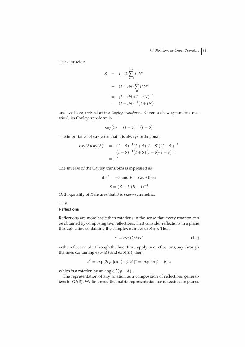
Rn(θ) = n⊗ n + cos θ(I − n⊗ n) + sin θn
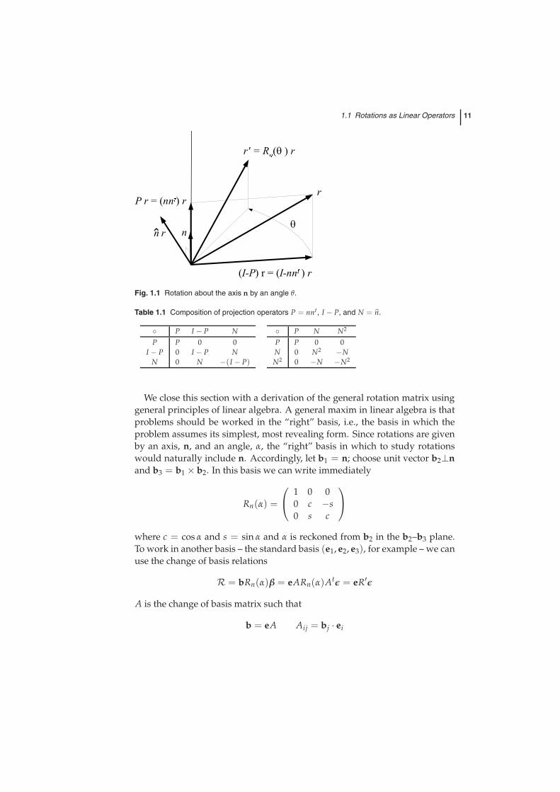
and we now proceed to justify this. Let P represent the operator relative to thestandard basis which projects a vector onto the axis of rotation (Fig. 1.1)
P = nnt
P has the property that, for any r, Pr is a multiple of n
Pr = nntr = λn λ = ntr
and P is idempotent
P2 = (nnt)(nnt) = n(ntn)nt = nnt = P
I − P then represents the operator which projects a vector onto the plane nor-mal to n because for any r
nt(I − P)r = ntr− ntnntr = 0
and(I − P)2 = I − P− P + P2 = I − P
Let N = n. Any rotation of r through an angle θ leaves Pr invariant androtates (I − P)r by an angle θ in the plane spanned by (I − P)r, n× r. Thusthe rotation is given by r′ = Rn(θ)r with
Rn(θ) = nnt + cos θ(
I − nnt)+ sin θ N
It is easy to show that the operators P, I− P, N form a closed system definedby Table 1.1. Here we sketch the proof of one entry as an illustration
N2r = n× (n× r) = (r · n)n− r = (P− I)r
The relations in Table 1.1 can be used to recast the rotation operator entirelyin terms of N,
R = I + sin θN + (1− cos θ)N2 (1.2)
1.1 Rotations as Linear Operators 11
Fig. 1.1 Rotation about the axis n by an angle θ.
Table 1.1 Composition of projection operators P = nnt, I − P, and N = n.
P I − P NP P 0 0
I − P 0 I − P NN 0 N −(I − P)
P N N2
P P 0 0N 0 N2 −NN2 0 −N −N2
We close this section with a derivation of the general rotation matrix usinggeneral principles of linear algebra. A general maxim in linear algebra is thatproblems should be worked in the “right” basis, i.e., the basis in which theproblem assumes its simplest, most revealing form. Since rotations are givenby an axis, n, and an angle, α, the “right” basis in which to study rotationswould naturally include n. Accordingly, let b1 = n; choose unit vector b2⊥nand b3 = b1 × b2. In this basis we can write immediately
Rn(α) =
1 0 00 c −s0 s c
where c = cos α and s = sin α and α is reckoned from b2 in the b2–b3 plane.To work in another basis – the standard basis (e1, e2, e3), for example – we canuse the change of basis relations
R = bRn(α)β = eARn(α)Atε = eR′ε
A is the change of basis matrix such that
b = eA Aij = bj · ei
12 1 Rotations
so column j of A contains the components bj of vector bj in the basis e (bj =ebj). That is
A = (b1 b2 b2)
Thus
R′ = (b1 b2 b3)
1 0 00 c −s0 s c
bt1
bt2
bt3
= b1bt
1 + c(b2bt2 + b3bt
3) + s(b3bt2 − b2bt
3)
Now we use the identitiesb1 = n,
I = b1bt1 + b2bt
2 + b3bt3
andb1 = b3bt
2 − b2bt3
to recoverR = nnt + c(I − nnt) + sN (1.3)
1.1.4The Cayley Transform
Equation (1.2) can be written in terms of t = tan 12 θ by using the identities
sin θ =2t
1 + t2 1− cos θ =2t2
1 + t2
Thus
R = I +2t
1 + t2 N +2t2
1 + t2 N2
This form of R leads to the Cayley transform of R and yet another form of therotation matrix which plays an important role in numerical calculations. Weneed the series expansion
11 + t2 =
∞
∑n=0
(−1)nt2n
and the results obtained from Table 1.1,
N2n = (−1)n+1N2
N2n+1 = (−1)nN
1.1 Rotations as Linear Operators 13
These provide
R = I + 2∞
∑n=1
tnNn
= (I + tN)∞
∑0
tnNn
= (I + tN)(I − tN)−1
= (I − tN)−1(I + tN)
and we have arrived at the Cayley transform. Given a skew-symmetric ma-trix S, its Cayley transform is
cay(S) = (I − S)−1(I + S)
The importance of cay(S) is that it is always orthogonal
cay(S)cay(S)t = (I − S)−1(I + S)(I + St)(I − St)−1
= (I − S)−1(I + S)(I − S)(I + S)−1
= I
The inverse of the Cayley transform is expressed as
if St = −S and R = cayS then
S = (R− I)(R + I)−1
Orthogonality of R insures that S is skew-symmetric.
1.1.5Reflections
Reflections are more basic than rotations in the sense that every rotation canbe obtained by composing two reflections. First consider reflections in a planethrough a line containing the complex number exp(ıφ). Then
z′ = exp(2ıφ)x∗ (1.4)
is the reflection of z through the line. If we apply two reflections, say throughthe lines containing exp(ıφ) and exp(ıψ), then
z′′ = exp(2ıψ)[exp(2ıφ)z∗]∗ = exp[2ı(ψ− φ)]z
which is a rotation by an angle 2(ψ− φ).The representation of any rotation as a composition of reflections general-
izes to SO(3). We first need the matrix representation for reflections in planes
14 1 Rotations
in R3 and the approach used to derive (1.3) also yields the matrix representa-tion for a reflection. The appropriate basis includes a normal n to the plane ofreflection
b1 = n b2⊥n and b3 = b1 × b2
Then the reflection is represented by (M for mirror)
M =
−1 0 00 1 00 0 1
and use of the change of basis matrix to the standard basis gives
Mn = (b1 b2 b3)
−1 0 00 1 00 0 1
bt1
bt2
bt3
= −b1bt
1 + b2bt2 + b3bt
3
and using b1 = n and I = b1bt1 + b2bt
2 + b3bt3 we obtain
Mn = I − 2nnt
The invariant form of the reflection operator is
Mn = I − 2n⊗ n
Now one can show that every rotation is the product of two reflections. Letthe rotation be Rn(α). Choose unit vectors q, p such that
p · n = 0 q · n = 0 and p · q = cos12
α
The product of reflections in q and p is
A = MpMq = I − 2p⊗ p− 2q⊗ q + 4 cos12
αp⊗ q
It is easily verified thatAn = n
n · Ap = n · Aq = 0,
p · Ap = −1 + 2 cos2 12
α = cos α
andq · Aq = cos α
which shows thatMpMq = Rn(α)

1.1 Rotations as Linear Operators 15
1.1.6Euler Angles
The specification of a rotation by axis and angle is convenient and subject to di-rect geometrical interpretation. It is, however, inconvenient as a basis for rigidbody dynamics because of redundancy. Any rotation matrix can be specifiedby three parameters (there are nine entries in the orthogonal matrix and sixconstraints imposed on the inner products of the columns). The redundancyarises because all three components of the axis are used as parameters eventhough only two are independent. The correspondence is also double-valuedin that n, α yield the same rotation as −n, −α. We now consider the Eulerangles which provide a three-parameter specification of a rotation.
Fig. 1.2 Definition of the Euler angles φ, θ, ψ.
The Euler angle parameterization of a rotation is the composite of three in-termediate rotations. The rotations are defined relative to the standard basise, and the effect of the intermediate rotations on this basis will be denoted byprimes (Fig. 1.2).
1. Rotate about e3 by an angle φ taking e1,e2 to e′1,e′2 and leaving e′3 = e3.
2. Rotate about e′1 by an angle θ taking e′2,e′3 to e′′2 ,e′′3 and leaving e′′1 = e′1.
3. Rotate about e′′3 by an angle ψ taking e′′1 ,e′′2 to e1,e2 and leaving e = e′′3 .
The angles φ, θ, ψ are sometimes called the angles of precession, nutation, andspin, respectively.
The intermediate rotations have the following matrix representations:
e′ = e
cos φ − sin φ 0sin φ cos φ 0
0 0 1
= eRe3(φ)
16 1 Rotations
e′′ = e′
1 0 00 cos θ − sin θ
0 sin θ cos θ
= e′Re1(θ)
and
e = e′′
cos ψ − sin ψ 0sin ψ cos ψ 0
0 0 1
= e′′Re3(ψ)
The composite rotation is
e = eRe3(φ)Re1(θ)Re3(ψ) = eR(φ, θ, ψ)
The operator is represented by the fixed basis e by using
R = eε = eR(φ, θ, ψ)ε.
The matrix products yield
R(φ, θ, ψ) = (1.5)
cos φ cos ψ− sin φ cos θ sin ψ − cos φ sin ψ− sin φ cos θ cos ψ sin φ sin θsin φ cos ψ + cos φ cos θ sin ψ − sin φ sin ψ + cos φ cos θ cos ψ − cos φ sin θ
sin θ sin ψ sin θ cos ψ cos θ
Given a rotation parameterized by the rotation angle α and rotation axis n, theEuler angle parameterization can be found as follows:
cos θ = Rn(α)(e3) · e3
cos φ = (e3 ×Rn(α)(e3)) · e1/ sin θ
cos ψ = (e3 ×Rn(α)(e3)) · Rn(α)(e2)/ sin θ
This conversion is not possible if sin θ = 0. In that case the Euler angle param-eterizations is not unique – φ and ψ cannot be separated.
There are many ways to represent a rotation as successive rotations aboutintermediate axes. For example, in aeronautics and astronautics one uses aparameterization dubbed yaw, pitch, and roll defined by the following:
1. Rotate about e3 by the yaw angle ψ.
2. Rotate about e′2 by the pitch angle θ.
3. Rotate about e′′1 by the roll angle φ.
In fact [3] there are 12 possible rotation sequences each defining a variantof the Euler angles. These are labeled by n1 − n2 − n3 corresponding to therotation
e = eRen1Re′n2
Re′′n3
1.2 Quaternions 17
The Euler angle parameterization discussed here would be labeled 3− 1− 3while yaw, pitch, and roll would be 3 − 2 − 1. There are 27 possible n1 −n2 − n3 combinations but it is necessary that n1 = n2 and n2 = n3 and 12combinations survive
1− 2− 1 2− 1− 2 3− 1− 31− 3− 1 2− 3− 2 3− 2− 31− 2− 3 2− 3− 1 3− 1− 21− 3− 2 2− 1− 3 3− 2− 1
1.2Quaternions
This section introduces a new number systems called quaternions which are in-timately connected to three-dimensional rotations (we have already seen thatcomplex numbers are intimately connected to plane rotations). As a prelude,the construction of more familiar number systems will be reviewed. Quater-nions will then seem quite natural. A good reference for these matters is [4].
We begin with the integers, Z. In Z we can add, multiply, and subtract butthere is no division. In other words, there is no multiplicative inverse in Z ofany integers other than±1. To obtain multiplicative inverses we need rationalnumbers, traditionally denoted by Q (for quotients). They are constructed asequivalence classes of ordered pairs of integers (n, m), m = 0, based on theequivalence relation
(n, m) ∼ (p, q), if and only if nq = mp
The equivalence classes are the sets
[(n, m)] = (p, q)|(p, q) ∼ (n, m)which is merely an abstract way to declare that rational numbers should bereduced to lowest terms. Having made the distinction between the pairs andthe equivalence classes we will now dispense with the square brackets fornotational simplicity. The operations of addition and multiplication of rationalnumbers are defined by
(n, m) + (p, q) = (nq + mp, mq)
(n, m)(p, q) = (np, mq)
Now every pair (n, m) has an additive inverse (−n, m)
(n, m) + (−n, m) = (0, m)
and, if n = 0 a multiplicative inverse (m, n)
(n, m)(m, n) = (1, 1)
18 1 Rotations
This is quite transparent when translated to grade school notation
(n, m) ↔ nm
The rational numbers are incomplete in the sense that there is no rationalnumber which represents the hypotenuse of a right triangle having unit legs.The real numbers R are constructed from pairs of sets of rational numbers,called Dedekind cuts,
(D1, D2), D1 and D2 ⊂ Q
which have the following four properties: each x ∈ D1 is less than everyy ∈ D2, D1 has no maximum element,
x ∈ D1 and y < x then y ∈ D1
andx ∈ D2 and y > x then y ∈ D2
For example, letD1 = r ∈ Q|r2 < 2
and let D2 be the set complement of D1 in Q . The Dedekind cut (D1, D2)represents the real number
√2.
The real numbers are incomplete in the sense that there is no solution in R
to the polynomial equationx2 + 1 = 0
We obtain an algebraically complete number system, the complex numbers C,from ordered pairs of real numbers
z = (x, y) x and y ∈ R
with addition and multiplication defined as
(x, y) + (u, v) = (x + u, y + v)
and(x, y)(u, v) = (xu− yv, xv + yu)
There is also a new operation, multiplication of a complex number by a realnumber:
a(x, y) = (a, 0)(x, y) = (ax, ay)
This appears more familiar in high school notation
(x, y)↔ x + ıy
1.2 Quaternions 19
The Irish mathematician Rowan Hamilton struggled in vain to extend com-plex numbers to three dimensions. Eventually he realized that it is neces-sary to go to four dimensions and he invented a new number system calledthe quaternions. We will introduce quaternions, H for Hamilton, as orderedpairs of complex numbers. Although Hamilton did not use the ordered pairconstruction for quaternions, he was the inventor of the pair construction forcomplex numbers. A quaternion, then, is an ordered pair of complex numbers
q = (z1, z2) z1 and z2 ∈ C
with addition and multiplication defined by
(z1, z2) + (w1, w2) = (z1 + w1, z2 + w2)
(z1, z2)(w1, w2) = (z1w1 − z2w∗2, z1w2 + z2w∗1)
anda(z, w) = (a, 0)(z, w) = (az, aw) a ∈ R
It turns out that multiplication is not commutative. That is, in general
rq = qr
We shall denote quaternions with sans serif typeface as in the last equation.This construction by pairs ties in nicely with the constructions of the ra-
tional, real, and complex numbers but is not the traditional approach. If wesingle out three special pairs and attach Hamilton’s notation to them
i = (ı, 0) j = (0, 1) k = (0, ı)
and identify(a, 0)↔ a a ∈ R
then we find
(q0 + ıq1, q2 + ıq3) = q0 + q1i + q2j + q3k qi ∈ R
which is the form Hamilton used to express quaternions. This form makes itquite clear that quaternions are a four-dimensional generalization of complexnumbers.
The quaternions i, j,k satisfy the following relations:
i2 = j2 = k2 = ijk = −1 (1.6)
These are the rules Hamilton inscribed on Broome Bridge in Dublin on Octo-ber 16, 1843 [5].
20 1 Rotations
In the language of abstract algebra, the quaternions form a noncommuta-tive, normed division algebra over R. The eight-dimensional octonians O [5]can be constructed from pairs of quaternions but there the chain ends. Theonly normed division algebras over R are R, C, H, and O.
1.2.1Quaternion Algebra
This section summarizes the essentials of the algebra of quaternions. First weexpress the basic operations in the i, j,k form. Addition becomes
(q0 + q1i + q2j + q3k) + (p0 + p1i + p2j + p3k)
= (q0 + p0) + (q1 + p1)i + (q2 + p2)j + (q3 + p3)k
and multiplication becomes
(q0 + q1i + q2j + q3k)(p0 + p1i + p2j + p3k) = q0 p0 − q1 p1 − q2 p2 − q3 p3
+ (q0 p1 + q1 p0 + q2 p3 − q3 p2)i
+ (q0 p2 + q2 p0 + q3 p1 − q1 p3)j
+ (q0 p3 + q3 p0 + q1 p2 − q2 p1)k
There are many patterns in this last expression and they will become clear bythe end of the next section.
Given q = q0 + q1i + q2j + q3k, q0 is called the scalar part of q
S(q) = q0
and q1i + q2j + q3k is called the vector part of q
V(q) = q1i + q2j + q3k
The conjugate of q isq = q0 − q1i− q2j− q3k
The square of the norm of q is
|q|2 = qq = q20 + q2
1 + q22 + q2
3 ∈ R
where we have taken the liberty of identifying a real number a and the quater-nion q with S(q) = a, V(q) = 0. The inverse of q is, when |q| = 0,
q−1 =1|q|2 q
Clearly qq−1 = 1 + 0i + 0j + 0k. Note also that qp = pq and (qp)−1 = p−1q−1.
1.2 Quaternions 21
1.2.2Quaternions as Scalar–Vector Pairs
At this point we have two ways to express quaternions – the complex numberpair form and the i, j, k form. There is a third way which is convenient foranyone accustomed to vector algebra. This third way represents quaternionsas scalar–vector pairs
q0 + q1i + q2j + q3k↔ (q0, v) with v = q1e1 + q2e2 + q3e3
In this way, the quaternion algebra is expressed as
(q0, u) + (p0, v) = (q0 + p0, u + v)
(q0, u)(p0, v) = (q0 p0 − u · v, q0v + p0u + u× v)
(q0, u) = (q0,−u)
|(q0, u)|2 = q20 + u · u
(q0, u)−1 =1
q20 + u · u
(q0,−u)
A perusal of the multiplication formula now reveals the patterns to be ele-ments of the scalar and vector products.
A pure quaternion (0, u) is one with zero scalar part and a unit quaternionhas unit norm qq = 1. The product of two pure quaternions encapsulates thescalar and vector products
(0, u)(0, v) = (−u · v, u× v)
1.2.3Quaternions as Matrices
Complex numbers can be represented as 2× 2 matrices with real entries. Let
J =(
0 −11 0
)and note that J2 = −I. Then Z = aI + bJ and W = cI + dJ
satisfy the rules for addition and multiplication of complex numbers
Z + W = (a + c)I + (b + d)J
ZW = (aI + bJ)(cI + dJ) = (ac− bd)I + (ad + bc)J
Similarly, quaternions can be represented as 2× 2 matrices of complex num-bers. If
z1 = q0 + ıq1 z2 = q2 + ıq3
w1 = r0 + ır1 w2 = r2 + ır3

22 1 Rotations
then the correspondences
Q1 =(
z1 z2−z∗2 z∗1
)↔ q0 + q1i + q2j + q3k
and
Q2 =(
w1 w2−w∗2 w∗1
)↔ r0 + r1i + r2j + r3k
are preserved by the matrix product
Q1Q2 ↔ (q0 + q1i + q2j + q3k)(r0 + r1i + r2j + r3k)
The quaternion product is linear in the components of each factor. Thisallows us to express the quaternion operations in terms of linear operationson R4. If we associate
q = q0 + q1i + q2j + q3k ↔ q =
q0q1q2q3
and
p = p0 + p1i + p2j + p3k↔ p =
p0p1p2p3
then left multiplication by q is represented by
L(q) =
q0 −q1 −q2 −q3q1 q0 −q3 q2q2 q3 q0 −q1q3 −q2 q1 q0
(1.7)
that is,qp ↔ L(q)p
This is expressed explicitly in a component form
q0 −q1 −q2 −q3q1 q0 −q3 q2q2 q3 q0 −q1q3 −q2 q1 q0
.
p0p1p2p3
=
q0 p0 − q1 p1 − q2 p2 − q3 p3q0 p1 + q1 p0 + q2 p3 − q3 p2q0 p2 + q2 p0 + q3 p1 − q1 p3q0 p3 + q3 p0 + q1 p2 − q2 p1
Right multiplication by q is represented by
R(q) =
q0 −q1 −q2 −q3q1 q0 q3 −q2q2 −q3 q0 q1q3 q2 −q1 q0
(1.8)

1.2 Quaternions 23
andpq ↔ R(q)p
These are the representations of the left and right translations Lq and Rq onthe Lie group S3 ∼= H1 (Appendix C).
Since LpLp = Lpq, it follows that
L(p)L(q) = L(pq)
There is the analogous result for right multiplication
R(p)R(q) = R(qp)
L(p) and R(p) have the following properties:
L(q)p = −L(p)q if qt p = 0
R(q)p = −R(p)q if qt p = 0
L(q) = L(q)t
L(q)L(q) = (qtq)I
R(q)R(q) = (qtq)I
If q ∈ H1 then R(q) and L(q) are orthogonal matrices. These relations arediscussed and applied in [6, 7]. This correspondence is a generalization of thev ↔ −→
M correspondence of R3 and so(3).
1.2.4Rotations via Unit Quaternions
Quaternions are useful in rigid body dynamics because they provide succinctexpressions for quantities which can be rather unwieldy in matrix form. Agood example is the composition of rotations which is a simple quaternionproduct. Rotations are effected in the quaternions by means of unit quater-nions. We denote the set of all unit quaternions by H1.
Let r = (0, v) be a pure quaternion and q = (q0, q) be a unit quaternion. Let
r′ = qrq−1 = qrq
Now we compute
r′ = (0, [q20 − q · q]v + 2v · qq + 2q0q× v)
and observe that if an angle θ and a unit vector n are defined by
q0 = cos12
θ and q ≡ (q1, q2, q3) = sin12
θ n
24 1 Rotations
thenr′ = (0, [1− cos θ]nn · v + cos θv + sin θn× v)
which reproduces the effect ofRn(θ) on the vector part of r. The qi arise mostnaturally in the context of quaternions. They were, however, introduced muchearlier by Euler and Rodrigues. For that reason they are sometimes called theEuler parameters or Euler–Rodrigues parameters.
Now it is natural to ask how the rotation matrix and the quaternion arerelated. First, let us express the rotation matrix R = Rn(θ) explicitly in termsof the components of n and the rotation angle via c = cos θ, s = sin θ,
R =
(1− c)n21 + c (1− c)n1n2 − sn3 (1− c)n1n3 + sn2
(1− c)n2n1 + sn3 (1− c)n22 + c (1− c)n2n3 − sn1
(1− c)n3n1 − sn2 (1− c)n3n2 + sn1 (1− c)n23 + c
(1.9)
Then, to express R in terms of the quaternion components qi, we use the iden-tities
c = q20 − q2
1 − q22 − q2
3 1− c = 2(1− q20) (1− c)ninj = 2qiqj
andsn = 2q0q.
Thus
R =
q20 + q2
1 − q22 − q2
3 2(q1q2 − q0q3) 2(q1q3 + q0q2)2(q2q1 + q0q3) q2
0 − q21 + q2
2 − q23 2(q2q3 − q0q1)
2(q3q1 − q0q2) 2(q3q2 + q0q1) q20 − q2
1 − q22 + q2
3
(1.10)
Note that quaternions q and −q correspond the same rotation matrix.Apart from its intrinsic interest, this expression is of practical importance
because it is a purely algebraic version of the rotation matrix. No transcen-dental functions are involved. This is relevant when computing requirementsare an issue.
The rotation defined by quaternion (q0, q) can also be expressed in the axis-angle form as
Rn(θ) = 2q⊗ q + (q20 − q · q)I + 2q0q q = sin
12
θ n
The process can be reversed. That is, given a rotation matrix, R, one canconstruct the components of the associated quaternion. Let τ = Trace(R) –the sum of the diagonal elements of R. From (1.9) we find
τ = 1 + 2 cos θ or cos θ =12(τ− 1) (1.11)
1.2 Quaternions 25
andq0 = cos
12
θ =12
√τ + 1. (1.12)
The vector part of the quaternion is found from the off-diagonal elements of R
q1 =1
4q0(R32 − R23) (1.13)
q2 =1
4q0(R13 − R31) (1.14)
q3 =1
4q0(R21 − R12) (1.15)
This may be expressed in matrix notation as
R− Rt = 4q0V(q)
Quaternions also handle reflections concisely. To reflect through the planewith unit normal n we have
(0, n)(0,−r)(0,−n) = (0, r− 2nn · r)
Conjugation applied to a pure quaternion is the same as negation. Thereforethe reflection operation is expressed in a slightly simpler form as
(0, n)(0, r)(0, n) = (0, r− 2nn · r)
Let two reflections be defined by the unit vectors n and m. The rotationdetermined by the composition of the two reflections is simply
(0, n)(0, m) = (−n ·m,−n×m) = −(cos θ, sin θn×m‖n×m‖ )
where θ is the angle between n and m. Therefore the angle of rotation is twicethe angle between the unit vectors and the axis of rotation is parallel to n×m(recall that rotations defined by quaternions q and −q are the same).
1.2.5Composition of Rotations
The composition of two rotations is itself a rotation because the product oftwo elements of SO(3) is itself in SO(3). Now we wish to inquire about therotation axis and rotation angle for the composite of two rotations.
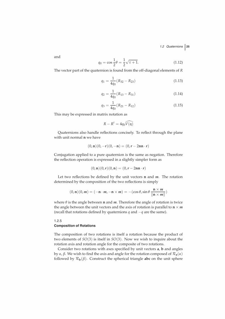
Consider two rotations with axes specified by unit vectors a, b and anglesby α, β. We wish to find the axis and angle for the rotation composed ofRa(α)followed by Rb(β). Construct the spherical triangle abc on the unit sphere
26 1 Rotations
Fig. 1.3 Defining figure for the Rodrigues spherical triangle.
Fig. 1.4 A sequence of finite rotations taking point a to a′, then to a′′
and then back to a illustrating the Rodrigues triangle.
shown in Fig. 1.3. The angles a and b are half the rotation angles and theorientation is such that rotation about a would bring arc ac toward arc ab. Wewill refer to this triangle as the Rodrigues triangle after Olinde Rodrigues whodiscovered the construction [8].
1.2 Quaternions 27
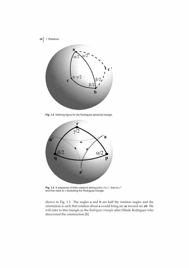
Fig. 1.5 A sequence of finite rotations of a cube: 180 about n =[0 1/2
√3/2] followed by 180 about k = [0 0 1]. The composite rota-
tion is about i = [1 0 0] by 60 as the shown by the Rodrigues sphericaltriangle displayed in the last panel.
The rotation axis and angle for the composite rotation can be obtained by anelegant geometrical argument [9–11]. Rotate arc ac about a by angle α takingpoint c to c′. Then rotate arc bc′ about axis b by angle β. This returns c′ to cthus showing that c is fixed under the composite rotation and must lie on theaxis of rotation. In more formal terms, consider the reflections Ma′ ,Mb′ , andMc′ (using the polar triangle notation established in Appendix A). We knowthat reflections preserve lengths of vectors and therefore reflections map theunit sphere into itself. The relation between reflections and rotations provides
Ra(α) = Mc′Mb′
Rb(β) = Ma′Mc′
and therefore
Rb(β)Ra(α) = Ma′Mc′Mc′Mb′
= Ma′Mb′
= R−c(2π− γ)
= Rc(γ)
It is instructive to use quaternions to calculate the composite rotation angle.Let the rotations be represented by the unit quaternions p = (cos 1
2 α, sin 12 αa)
and q = (cos 12 β, sin 1
2 βb) and let a · b = cos φ . The effect of rotation 1 fol-lowed by rotation 2 is
r′ = q(prp−1)q−1 = (qp)r(qp)−1
28 1 Rotations
so that the composition is obtained from the product r = qp
qp =(
cos12
α cos12
β− sin12
α sin12
β cos φ, (1.16)
cos12
α sin12
β b + cos12
β sin12
α a + sin12
α sin12
β a× b)
Thuscos
12
γ = S(qp) = cos12
α cos12
β− sin12
α sin12
β cos φ
Now, referring to Appendix A, Eq. (A.15), we find that
cos C = − cos12
α cos12
β + sin12
α sin12
β cos φ
Thereforecos
12
γ = − cos C
orC = π − 1
2γ
and the construction is validated. With γ in hand, the axis of the compositerotation is simply
n = V(qp)/ sin12
γ
The Rodrigues triangle construction may also be given by the followingequivalent description. Refer to the spherical triangle constructed in Fig. 1.4.
Given a spherical triangle with vertices p, q, and r and vertex angles α/2,β/2 and γ/2 successive rotations about p by angle α, q by β, and r by γ yieldthe identity transformation.
Rr(γ)Rq(β)Rp(α) = Mq′Mp′Mp′Mr′Mr′Mq′
= I
Example 1.2 An illustration of the composition of rotations of a cube and the associ-ated Rodrigues spherical triangle is shown in Fig. 1.5. The analytic expression of thatcomposition is
Rk(π)Rn(π) = R−i(2π− π/3) = Ri(π/3)
Note the orientation of the Rodrigues triangle. ♦
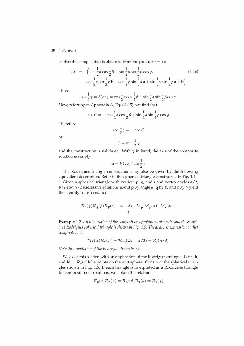
We close this section with an application of the Rodrigues triangle. Let a, b,and b′ = Ra(α)b be points on the unit sphere. Construct the spherical trian-gles shown in Fig. 1.6. If each triangle is interpreted as a Rodrigues trianglefor composition of rotations, we obtain the relation
Ra(α)Rb(β) = Rb′(β)Ra(α) = Rc(γ)
1.3 Complex Numbers 29
Fig. 1.6 Transposition of rotations about a, b, and b′ = Ra(α)b.
This is referred to as Rodrigues’ transposition of rotations [3, 12] or rotationreversal [13].
Example 1.3 This relation can be used to clarify the order of factors occurring inthe operator and matrix versions of the Euler angle parameterization. In operatornotation,
R = Re′′3(ψ)Re′1
(θ)Re3(φ)
which can be subjected to transpositions to obtain
R = Re′1(θ)Re′3
(ψ)Re3(φ) = Re′1(θ)Re3(φ)Re3(ψ) = Re3(φ)Re1(θ)Re3(ψ)
This leads immediately, in the notation of Section 1.1.6, to the representation
R = eRe3(φ)Re1(θ)Re3(ψ)ε. ♦
1.3Complex Numbers
In this section we describe rotations parameterized by Möbius transforma-tions of the complex plane. The development begins by recasting the repre-sentation of quaternions as 2× 2 matrices with complex entries. Section 1.2.3examined a mapping from the quaternion components to the complex entriesin the matrices. Here we explore a different mapping which will lead to inter-esting connections between rotations and complex functions.4
4) There are actually 24 such mappings which are isomorphisms.
30 1 Rotations
1.3.1Cayley–Klein Parameters
Define the following matrices.5
J1 =(
0 ıı 0
)J2 =
(0 −11 0
)J3 =
(ı 00 −ı
)
These matrices obey the quaternion multiplication rules (1.6), namely J21 =
J22 = J2
3 = J1 J2 J3 = −I, and the quaternions are mapped to the set of real,linear combinations of I, J1, J2, J3,
q0 + q1i + q2j + q3k ↔ q0 I + q1 J1 + q2 J2 + q3 J3 =(
q0 + ıq3 −q2 + ıq1q2 + ıq1 q0 − ıq3
)
It is easy to show that if p, q ∈ H are mapped to P, Q, then p + q and pq
are mapped to P + Q and PQ. Conjugation in the quaternions corresponds totaking the adjoint of the associated matrix
q ↔ Q† = (Qt)∗
In other words, H is isomorphic to the algebra over R of complex 2× 2 matri-ces of the form (
u v−v∗ u∗
)
Now if
Q =(
q0 + ıq3 −q2 + ıq1q2 + ıq1 q0 − ıq3
), q = q0 + q1i + q2j + q3k
thendet Q = q2
0 + q21 + q2
2 + q23 = |q|2
which shows that the subalgebra of unit quaternions, H1, is isomorphic to thesubgroup of GL(2, C) in which each element satisfies QQ† = I and det Q = 1.This group is called SU(2), the group of special unitary matrices of order 2.
Given the correspondence between SU(2) and H1 it follows that rotationscan be represented in SU(2) as follows. Let X be the matrix corresponding tothe pure quaternion r = (0, r), r = (x y x) and let q ∈ H1. Then
r ↔(
ız −y + ıxy + ıx −ız
)= X
andqrq ↔ QXQ†
5) These matrices are related to the Pauli matrices σi of quantumphysics by J1 = ıσ1, J2 = −ıσ2, and J3 = ıσ3.
1.3 Complex Numbers 31
In the context of rigid body mechanics the elements of the matrices in SU(2)are called the Cayley–Klein parameters. These parameters can be expressed interms of the Euler angles. From Eqs. (1.5) and (1.12–1.15) we obtain
4q20 = τ + 1 = (1 + cos θ)(1 + cos(φ + ψ)) = 4 cos2 1
2θ cos2 1
2(φ + ψ)
and
4q0q1 = sin θ(cos φ + cos ψ)
= sin θ
(cos
[12(φ + ψ) +
12(φ− ψ)
]+ cos
[12(φ + ψ)− 1
2(φ− ψ)
])
= 4 cos12
θ sin12
θ cos12(φ + ψ) cos
12(φ− ψ)
Thus
q0 = cos12
θ cos12(φ + ψ) (1.17)
q1 = sin12
θ cos12(φ− ψ) (1.18)
and similarly
q2 = sin12
θ sin12(φ− ψ) (1.19)
q3 = cos12
θ sin12(φ + ψ) (1.20)
With the identifications
α = q0 + ıq3, β = −q2 + ıq1, γ = −β∗, δ = α∗
the SU(2) representation of the rotation matrix becomes
(α β
γ δ
)=
(cos 1
2 θe12 ı(φ+ψ) ı sin 1
2 θe12 ı(φ−ψ)
ı sin 12 θe−
12 ı(φ−ψ) cos 1
2 θe−12 ı(φ+ψ)
)
1.3.2Rotations and the Complex Plane
We have considered rotations in the SO(3), H1, and SU(2) settings. The lastsetting we wish to consider is the complex plane with point at infinity. This isthe so-called Riemann sphere, C, the simplest of the compact Riemann surfaces.There is a one–one map, called the stereographic projection, from the unit sphereto C. Imagine the complex plane intersecting a unit sphere in its equator. Tomap the point r = (ξ η ζ) on the sphere to the complex plane, one draws a
32 1 Rotations
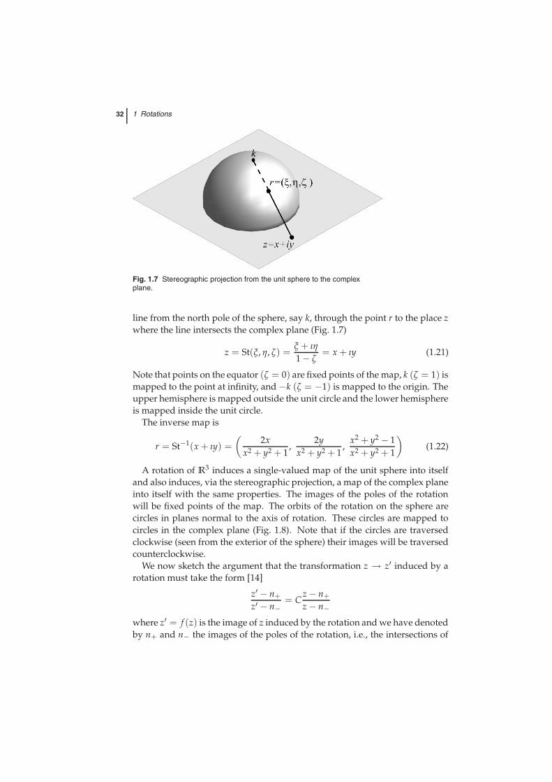
Fig. 1.7 Stereographic projection from the unit sphere to the complexplane.
line from the north pole of the sphere, say k, through the point r to the place zwhere the line intersects the complex plane (Fig. 1.7)
z = St(ξ, η, ζ) =ξ + ıη1− ζ
= x + ıy (1.21)
Note that points on the equator (ζ = 0) are fixed points of the map, k (ζ = 1) ismapped to the point at infinity, and −k (ζ = −1) is mapped to the origin. Theupper hemisphere is mapped outside the unit circle and the lower hemisphereis mapped inside the unit circle.
The inverse map is
r = St−1(x + ıy) =(
2xx2 + y2 + 1
,2y
x2 + y2 + 1,
x2 + y2 − 1x2 + y2 + 1
)(1.22)
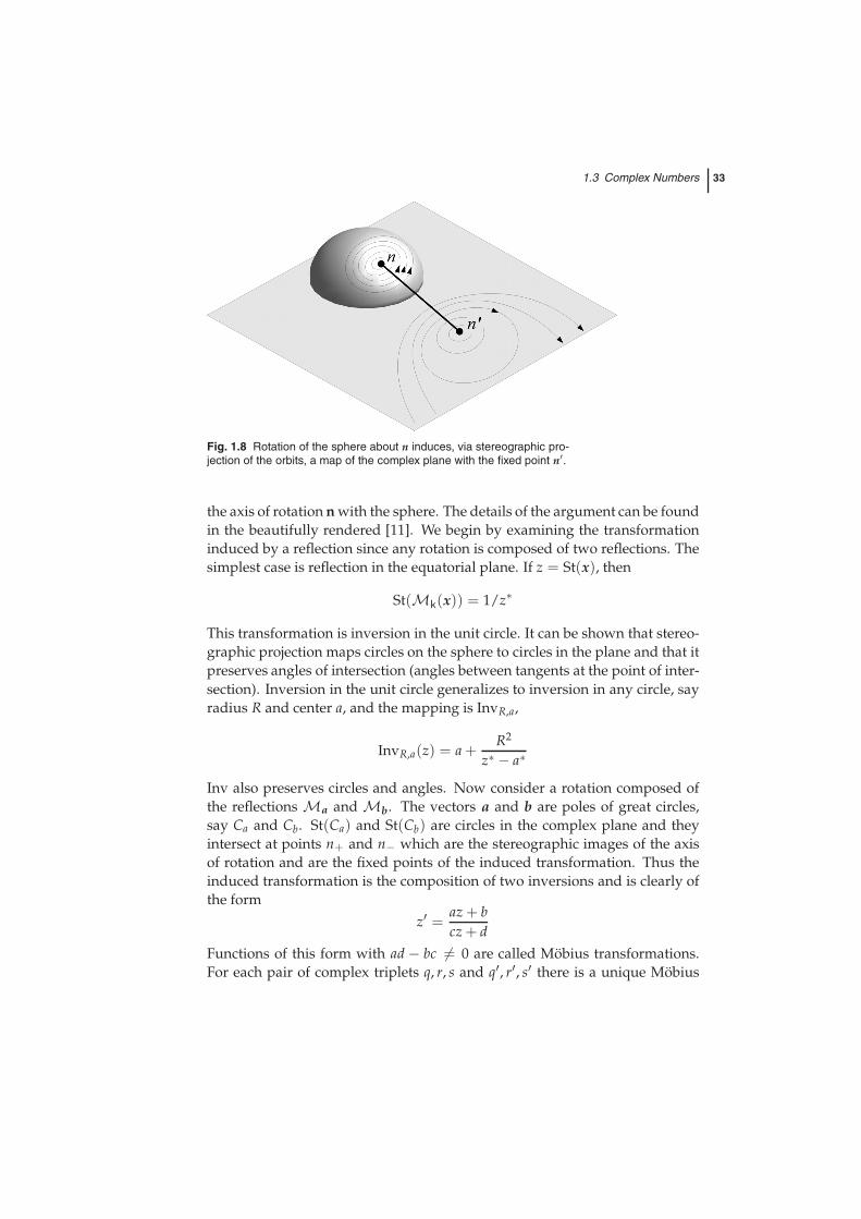
A rotation of R3 induces a single-valued map of the unit sphere into itselfand also induces, via the stereographic projection, a map of the complex planeinto itself with the same properties. The images of the poles of the rotationwill be fixed points of the map. The orbits of the rotation on the sphere arecircles in planes normal to the axis of rotation. These circles are mapped tocircles in the complex plane (Fig. 1.8). Note that if the circles are traversedclockwise (seen from the exterior of the sphere) their images will be traversedcounterclockwise.
We now sketch the argument that the transformation z → z′ induced by arotation must take the form [14]
z′ − n+
z′ − n−= C
z− n+
z− n−
where z′ = f (z) is the image of z induced by the rotation and we have denotedby n+ and n− the images of the poles of the rotation, i.e., the intersections of
1.3 Complex Numbers 33
Fig. 1.8 Rotation of the sphere about n induces, via stereographic pro-jection of the orbits, a map of the complex plane with the fixed point n′.
the axis of rotation n with the sphere. The details of the argument can be foundin the beautifully rendered [11]. We begin by examining the transformationinduced by a reflection since any rotation is composed of two reflections. Thesimplest case is reflection in the equatorial plane. If z = St(x), then
St(Mk(x)) = 1/z∗
This transformation is inversion in the unit circle. It can be shown that stereo-graphic projection maps circles on the sphere to circles in the plane and that itpreserves angles of intersection (angles between tangents at the point of inter-section). Inversion in the unit circle generalizes to inversion in any circle, sayradius R and center a, and the mapping is InvR,a,
InvR,a(z) = a +R2
z∗ − a∗
Inv also preserves circles and angles. Now consider a rotation composed ofthe reflections Ma and Mb. The vectors a and b are poles of great circles,say Ca and Cb. St(Ca) and St(Cb) are circles in the complex plane and theyintersect at points n+ and n− which are the stereographic images of the axisof rotation and are the fixed points of the induced transformation. Thus theinduced transformation is the composition of two inversions and is clearly ofthe form
z′ =az + bcz + d
Functions of this form with ad − bc = 0 are called Möbius transformations.For each pair of complex triplets q, r, s and q′, r′, s′ there is a unique Möbius
34 1 Rotations
transformation taking one to the other
z′ − q′
z′ − r′s′ − r′
s′ − q′=
z− qz− r
s− rs− q
If we choose q = n+, r = n−, and s = ∞
z′ − n+
z′ − n−=
z′∞ − n+
z′∞ − n−
z− n+
z− n−
By (1.21)
n+ =n1 + ın2
1− n3n− = −n1 + ın2
1 + n3
The image of the point at infinity in the complex plane, z′∞, is the stereographicprojection of the image of k under the rotation which is, in the standard basis,
Rn(χ)(k) =[(1− cos χ)nnt + cos χI + sin χn
]k
=
2(n1n3 sin2 12 χ + n2 sin 1
2 χ cos 12 χ)
2(n2n3 sin2 12 χ− n1 sin 1
2 χ cos 12 χ)
2n23 sin2 1
2 χ− sin2 12 χ + cos2 1
2 χ
=
2(q1q3 + q0q2)2(q2q3 − q0q1)2(q2
0 + q23)− 1
Stereographic projection yields
z′∞ = ı(n1 + ın2)(cos 1
2 χ + ı sin 12 χ)
(1− n23) sin2 1
2 χ
from which it follows that
C =z′∞ − n+
z′∞ − n−= e−ıχ
Now it is just a matter of algebra to show that
z′ = f (z) =αz + β
−β∗z + α∗
where
α = q0 + ıq3 β = −q2 + ıq1 (1.23)
are the Cayley–Klein parameters. The form of this function is not unique be-cause the numerator and denominator can be multiplied by a common factor
1.4 Summary 35
without affecting its value. In other words, there is an equivalence class offunctions which correspond to each rotation of the sphere. We have chosen,as is always possible if αδ− βγ = 0, the function satisfying
z′ = f (z) =αz + β
−β∗z + α∗αα∗ + ββ∗ = 1
These equivalence classes of functions are called normalized Möbius transfor-mations, Mo(C), and there is a one–one correspondence between them andmatrices in SU(2) (
u v−v∗ u∗
)↔ uz + v−v∗z + u∗
The correspondence yields an isomorphism. If A, B ∈ SU(2) and f , g ∈Mo(C) with A ↔ f , B ↔ g, then AB ↔ f g and A−1 ↔ f−1.
1.4Summary
Table 1.2 Summary of rotation parameterizations.
Object Typical element Group operation Representation ofrotation
H1 (q0, q) Quaternion multiply qrq
SU(2)(
q0 + ıq3 −q2 + ıq1q2 + ıq1 q0 − ıq3
)Matrix multiply AXA†
Mo(C) (q0 + ıq3)z− q2 + ıq1(q2 + ıq1)z + q0 − ıq3
Composition f (z)
SO(3) 2qqt + (q20 − q · q)I + 2q0q Matrix multiply R v
The aspects of the theory of rotations in R3 covered in this chapter are sum-marized in Table 1.2 . The first three objects are isomorphic but they each beara 2–1 relationship with SO(3). This state of affairs is sometimes expressedas “SU(2) is a double cover for SO(3).” This has profound implications inparticle physics where the duplicity represents spin.
We close this chapter with comment on the topology of the systems usedto represent rotations. H1, and hence SU(2), is homeomorphic to the three-dimensional sphere
S3 = [x ∈ R4|x · x = 1]
On the other hand, SO(3) is homeomorphic to S3 with antipodal points identi-fied. This is the projective space RP3 – the space of all lines through the originin R4. The former is simply connected (any loop can be contracted to a point)
36 1 Rotations
but the latter is not. In H1 or SU(2) it is possible, to “unwind” the loops whichproject to noncontractible loops in SO(3). For example, an arc from a point onS3 to its antipode projects to a closed loop in SO(3). This can actually be vi-sualized with strings attached to a rotated body and is very nicely illustratedin [10]. It is also related to the “waiter’s trick” described in [15]. If one holdsa tray on one’s outstretched, upturned hand one can rotate the tray by 360
using only motion of the wrist and the arm. The “trick” is that in doing sothe elbow winds up pointed skyward. A further rotation by 360 using onlymotions of the wrist and the arm restores the elbow to its original position.