Problems from Computer Aided Engineering Design Anupam Saxena and Birendra Sahay

Chapter I 1.1 A four-bar mechanism is shown in Fig. P1.1. Fixed pivots are given to be O2O4 = 20 cm. The input crank

O2A=10 cm and AB= BO4=25 cm. Trace the point path of point P for AP=50 cm. All links are rigid. 1.2 A Chebychev’s straight line linkage is shown in Fig. P1.2. Fixed pivots are given to be O2O4=20 cm.

O2A=25 cm and AB=10 cm and BO4=25 cm. Determine the path traced by the point P if BP=5 cm. All links are rigid.

1.3 A film advance mechanism is shown in Fig. P1.3 for a 35 mm camera. Link 2 is attached to the dc motor and rotates at a constant angular velocity. O2O4 are fixed pivots. Link 3 is extended and has a pin-end, which goes into the rectangular groove of the film, moves along a straight line by 35 mm and then lifts up to disengage from the film at the end of its motion. Design the mechanism by selecting suitable sizes of the linkages.

1.4 For the mechanism shown in Fig. P1.4, the input angle θ2=600, and the constant angular velocity ω2=5 radians/sec (CCW). If body 4 is in rolling contact with the ground, determine the velocity and acceleration of links 3 and 4 using kinematic coefficients. The links AB=25 cm, BC=15 cm, and radius of the rigid roller 4 is 12.5 cm.

Fig. P1.1 Fig. P1.2

2

Fig. P1.3 Fig. P1.4 1.5 Steps for design of compression springs for static loadings has been described earlier which can be easily

implemented on a computer using MatLab. (a) Extend the method for design of compression springs under fatigue loading. These types of springs are

used in IC engines, compressors, shock absorbers in vehicles etc. (b) Add modules to your computer program (make it interactive) to include design of extension springs,

torsion springs and leaf springs. 1.6 Write a computer program for selection of ball bearings. The program should include a look-up table

(Timken or SKF) for some standard bearings. It should calculate and check the bearing life under the given loading conditions.

1.7 Write an interactive computer program for complete design of short journal bearings. It is easy to use Ocvirk’s solution. The software should take into account the bearing material, type of lubricating oils and their viscosities and thermal considerations.

1.8 Shafts and axles are most commonly used mechanical components. They are designed to transmit power. They should be designed and checked for deflection and rigidity as well as static and fatigue strength for a given loading condition. Keyways, pins, splines and diameter changes introduce stress concentration. Make a computer program for design of shafts. Look up tables for material etc. will be helpful to the designer.

3

Chapter II 1. For the position vectors p1 (1,1), p2 (3,1), p3 (4,2), p4 (2,3), that defines a 2D polygon, develop a single

transformation matrix that

(a) reflects about the line x = 0, (b) translates by –1 in both x and y directions, and (c) rotates about the origin by 180o

using the transformations, determine the transformed position vectors. A viewing transformation matrix is given below. Find the Cartesian coordinates of the vanishing points along the three principal directions

[T] =

−−−−−−

1000

245.00612.0500.0

283.00707.00

141.00354.0866.0

2. Develop an algorithm to find the set of vertices making a regular 2D polygon. You may use only

transformations on points. Input parameters are the starting point p0 (0, 0), number of edges n, and length of edge l.

3. Prove that the transformation matrix

+−

+−

++−

=

100

01

1

1

2

01

2

1

1

2

2

2

22

2

t

t

t

tt

t

t

t

R

produces a pure rotation. Find equivalent θ. 4. Show that the reflection about an arbitrary line ax + by + c = 0 is given by

+−−

−−−−

22

22

22

122

02

02

babcac

baab

abab

5. Consider two lines L1: y = c and L2: y = mx+c. These two lines intersect at point C on y-axis. The angle θ

between these lines can be found easily. A point P (x1, y1) is first reflected through L1 and subsequently through L2. Show that this is equivalent to rotating the point P about the intersection point C by 2θ.

6. A point P (x, y) has been transformed to P*(x*, y*) by a transformation M . Find the matrix M .

4

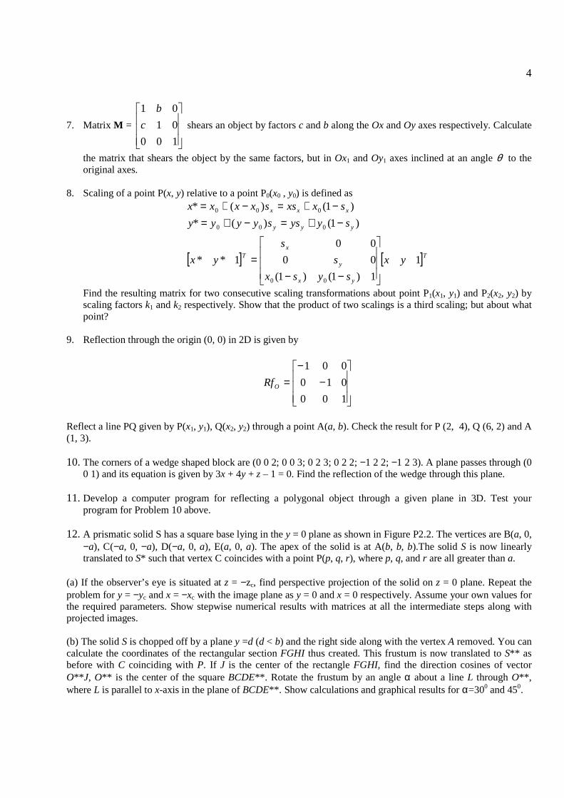
7. Matrix M =

100

01

01

c

b

shears an object by factors c and b along the Ox and Oy axes respectively. Calculate

the matrix that shears the object by the same factors, but in Ox1 and Oy1 axes inclined at an angle θ to the original axes.

8. Scaling of a point P(x, y) relative to a point P0(x0 , y0) is defined as

[ ] [ ]T

yx

y

xT

yyy

xxx

yx

sysx

s

s

yx

syyssyyyy

sxxssxxxx

1

1)1()1(

00

00

1**

)1()(*

)1()(*

00

000

000

−−=

−+=−+=−+=−+=

Find the resulting matrix for two consecutive scaling transformations about point P1(x1, y1) and P2(x2, y2) by scaling factors k1 and k2 respectively. Show that the product of two scalings is a third scaling; but about what point?

9. Reflection through the origin (0, 0) in 2D is given by

−−

=100

010

001

ORf

Reflect a line PQ given by P(x1, y1), Q(x2, y2) through a point A(a, b). Check the result for P (2, 4), Q (6, 2) and A (1, 3). 10. The corners of a wedge shaped block are (0 0 2; 0 0 3; 0 2 3; 0 2 2; −1 2 2; −1 2 3). A plane passes through (0

0 1) and its equation is given by 3x + 4y + z – 1 = 0. Find the reflection of the wedge through this plane. 11. Develop a computer program for reflecting a polygonal object through a given plane in 3D. Test your

program for Problem 10 above. 12. A prismatic solid S has a square base lying in the y = 0 plane as shown in Figure P2.2. The vertices are B(a, 0,

−a), C(−a, 0, −a), D(−a, 0, a), E(a, 0, a). The apex of the solid is at A(b, b, b).The solid S is now linearly translated to S* such that vertex C coincides with a point P(p, q, r), where p, q, and r are all greater than a.

(a) If the observer’s eye is situated at z = −zc, find perspective projection of the solid on z = 0 plane. Repeat the problem for y = −yc and x = −xc with the image plane as y = 0 and x = 0 respectively. Assume your own values for the required parameters. Show stepwise numerical results with matrices at all the intermediate steps along with projected images. (b) The solid S is chopped off by a plane y =d (d < b) and the right side along with the vertex A removed. You can calculate the coordinates of the rectangular section FGHI thus created. This frustum is now translated to S** as before with C coinciding with P. If J is the center of the rectangle FGHI, find the direction cosines of vector O** J, O** is the center of the square BCDE**. Rotate the frustum by an angle α about a line L through O**, where L is parallel to x-axis in the plane of BCDE**. Show calculations and graphical results for α=300 and 450.

5

Figure P2.2 13. A machine block is shown in the Figure P2.3. Using transformations, show the following graphical results.

Figure P2.3 Machine block.

(a) Orthographic projections. (b) The object is rotated about y-axis by an angle ϕ and then about x-axis through ψ. This is followed by a parallel projection on z = 0 plane to get a trimetric projection. For ϕ = 300 and 450, draw figures for trimetric projections when ψ takes on the values 30, 45, 60 and 90 degrees. Calculate the foreshortening factors for each of the positions. 14. For the component shown in Figure P2.3, Show the Cavalier and Cabinet projections for α = 30, 0, and – 45

degrees.

X Y

Z

O

B (a, 0, −a)

C (−a, 0, −a)

A (b, b, b)

D (−a, 0, a)

E (a, 0, a)

6

Chapter III 1. Find the parametric equation of an Archimedean spiral in a polar form. The largest and the smallest radii of

the spiral are 100 mm and 20 mm respectively. The spiral has two convolutions to reduce the radius from the largest to the smallest value.

2. Derive the equation in a parametric form of a cycloid. The cycloid is obtained as the locus of a point on the

circumference of a circle when the circle rolls without slipping on a straight line for one complete revolution. Assume the diameter of the circle to be 50 mm. Also, derive the parametric equation for the tangent and the normal at any generic point on the curve. Furthermore, fine the coordinates of the center of curvature of a generic point on the curve.

3. Fine the curvature and torsion of the following curves.

x = u, y = u2, z = u3

x = u, y = (1 + u)/u, z = (1 – u2)/u x = a(u – sin u), y = a(1 – cos u), z = bu

4. Find the biparametric equation of a plane bounded by a triangular region. The vertices of the triangle are A (a,

0, 0), B (0, b, 0), C (0, 0, c). 5. Derive the parametric equation of parabolic arch whose span is 150 mm and rise is 65 mm. 6. Derive the parametric equation of an equilateral hyperbola passing through a point P (15, 65). 7. Derive the parametric equation of an ellipse whose major and minor diameters are 150 mm and 75 mm

respectively. Furthermore, the major and minor diameters are conjugate diameters inclined to one another by 60 degrees. The major diameter is horizontal.

8. Find the parametric equation of a circle passing through three points p0, p1 and p2 lying on XY plane. Discuss

under what conditions your equation will fail to define a circle. 9. Find the equation for the skew distance (shortest distance) as well as the skew angle between a pair of skew

lines AB and CD. 10. For a line AB, specified in space, find the angle of this line from the XOY plane. Also, find the angle that the

projection of this line in the XOY planes makes with respect to X–axis. 11. Find the equation of the dihedral angle between two intersecting plane ABC and ABD in terms of coordinates

of points A, B, C and D. 12. Find the osculating, tangent and normal planes for the following curves a) x(u) = 3u, y(u) = 3u2, z(u) = 2u3

b) x(u) = a cos u, y(u) = a sin u, z(u) = b u Plot x(u), y(u), z(u) versus u for –1 ≤ u ≤ 1 and the curve r (u) = x(u) i + y(u) j + z(u) k for both curves.

13. If r (s) is an arc length parametrized curve such that torsion τ=0, and curvature κ is a constant, show that r (s)

is a circle. 14. Calculate the moving trihedron values as functions of u and plot the curvature and torsion for r (u) = (3u – u3,

3u2, 3u + u3) shown in the Figure P3.1 below.

7

Figure P3.1

15. Plot the curvature and torsion of the Viviani’s curve (intersection of a cylinder and a sphere). 16. Write a procedure to create Frenet Frame at any given point of a 3-D curve. 17. Write a procedure to calculate curvature and torsion of a 3 dimensional curve at a given point and also a

procedure to plot these shape parameters.

-2-1

01

20

12

3

-4

-2

0

2

40

12

3

8

Chapter IV 1. Consider a parametric cubic curve r (u) where

r (u) = F1 P0 + F2 P1 + F3 P’0 + F4 P’1 0 ≤ u ≤ 1 where F1 = 1 − 3u2 + 2u3, F2 = 3u2 – 2u3, F3 = u − 2u2 + u3, F4 = −u2 + u3

In some situations, data about P’0 and P’1 is not available, Instead, vectors P’’ 0 and P’’ 1 are known. In such cases, derive the expressions for all elements of K for the parametric equation to be written in the form r (u) = U K C where

U = [u3 u2 u 1], CT = [P0 P1 P’’ 0 P’’ 1] and K is the 4×4 matrix. 2. Given a parametric cubic curve whose geometric coefficients are [P0 P1 P’0 P’1] snip or trim the curve at u =

0.7 and reparametrize this segment so that 0 ≤ u ≤ 1. Find the relationship between the geometric coefficients of the sniped and original curves.

3. Derive the cubic Bézier curve in the matrix form, illustrating the control points, the curve shape, and the

blending functions through sketches. Derive also the expression for the tangent at any given point on the curve. Write a computer code to display a 3D cubic Bézier curve. The input shall be the control point coordinates. Shift any one of the given control points to a new location and show the change in shape on a plot. Output also the tangent value at any specific ‘u’ value given.

4. Consider a Bézier cubic curve obtained by a set of points P0, P1, P2 and P3. Assume that it is not possible to specify P1 and P2 but one can specify P*, the point of intersection of P0P1 and P2P3. The Bezier curve for P0, P*, P2 will be quadratic one. What will be the relation between P*, P0, P1, P2 and P3 so that the cubic as well the quadratic Bézier curves are identical ones.

5. A parametric cubic curve is to be fitted to pass through four points P0, P1, P2, P3. The first and last points P0, P3 are to be at u = 0 and u = 1 respectively. Points P1 and P2 are at u = 1/3 and u = 2/3 respectively. The equation of the curve is to be written in the form

r (u) = UM p P = [ ]

3

2

1

0

44434241

34333231

24232221

14131211

23 1

P

P

P

P

mmmm

mmmm

mmmm

mmmm

uuu

Show that the basis matrix is given by

Mp =

−−−−

−−

0001.0

1.04.59.05.5

4.51822.59.0

4.513.513.54.5

(a) Plot the curve passing through (0, 0), (1, 0), (1, 1),(0, 1) (b) A circular arc of radius 2 lies in the first quadrant. Write the co-ordinates of the 4 points that are equally

spaced on this arc. Calculate the point on the arc at u = ½ . How far does it deviate from the midpoint of the true quarter circle?

6. In the above example, let P2 and P3 be at u = α and u = β (α < β < 1). Re-derive the expression for the basis

matrix.

9

7. A 3-D parametric cubic curve has the start and end points at P0 (0, 0, 0) and P1 (1, 1, 1) and the end tangents are (1, 0, 0) and (0, 1, 0). (a) Find and draw the parametric equation of the curve segment. (b) If the end tangents have the magnitudes α and β, show some results of the variation in curve shape due to

changes in α, β. 8. The geometric matrix G of a parametric cubic curve defines a straight-line-segment if

G = [P0 P1 α( P1 – P0) β( P1 – P0)]

T Express the equation of the straight line as a cubic function in u. Tabulate and draw the points on the straight lines at intervals of ∆u = 0.01 from u = 0 to u = 1 in the following cases.

(a) α = β = 1 (b) α = β = –1 (c) α = 2, β = 4 (d) α = –2, β = – 4

At what values of u the trace of the line changes directions in each of the cases?

9. Show that a linear relationship v = au + b preserves the cubic form of the equations as well as the directions of tangent lines while reparametrizing. (b) For a = −1, b = 1, show that the direction of parametrization of r (u) is reversed.

10. Write a procedure to truncate a parametric cubic curve at two specified values of u and subsequently

reparametrize it. Test your program for a parametric cubic curve with a given set of end points P0 (1, 1, 1) and P1 (4, 2, 4) and the end tangents r u(0) = (1, 1, 0) and r u(1) = (1, 1, 1) truncated at (a) u = 0.25, and u = 0.75 (b) u = 0.333 and u = 0.667.

11. Write a procedure for blending a parametric cubic curve between two given such curves. Create a 2-D

numerical example to test your algorithm. Show the effect of changing the magnitudes of the tangent vectors at curve joints.

12. Find the expressions for the curvature at a point on a parametric cubic curve and a Bézier curve. Calculate the

curvatures at the end points of a Bézier curve having the control points (1, 1), (2, 3), (4, 6), (7, 1). Plot the Bézier curve along with its convex polygon.

13. A composite Bézier curve is to be obtained by joining two Bézier curves with control points at P0, P1, P2, P3

and Q0, Q1, Q2, Q3. Develop a procedure and check your results by taking a 2-D example. Modify your results by taking Q0, Q1, Q2, Q3, Q4 as control polygon for the second curve. (Hint: A condition for C0 continuity is Q0 = P3 and for C1 continuity is Q1 = (1 – λ)P2 + λP3, λ > 1).

14. Develop an algorithm for closed Bézier curves. Demonstrate through numerical 2-D examples. 15. Write a computer program implementing de Casteljau algorithm for cubic curves, over some interval u1 and

u2. Test your program with the points P0 = (6, − 5), P1 = (−6, 12), P2 = (−6, −14), P3 = (6, 5). Use de Casteljau algorithm to find the coordinates of points on the curve at u = 0.25, 1/3, 0.5, 2/3, 0.75, and 1. Plot the cubic curve.

16. Show, through an example that a Bézier curve is affine under both translation and rotation. You can choose

the above control points and rotate the axes by 45 degrees or translate the origin to (−2, −2).

10

17. Given a set of control points P0, P1, P2, P3 explain what happens when two of the control points are coincident. Give an example. Does the degree of the curve drop? Does the curve have a cusp at some control point? Does the curve have an inflexion at some control point?

18. Develop programs for drawing closed Bézier curves with C0 and C1 continuities. Give some illustrative

examples. 19. Show that the curvature of a planar curve is independent of the parametrization. That is, if r (u) = [x(u) y(u)]

is the curve, then a change of variables u = ϕ(v), where 0)( ≠vϕ& does not affect the curvature. 20. Let P0, P1, P2, P3 be given control points. Let us construct two quadratic curve segments Q1Q2 (r 1(u)) and

Q2Q3 (r 2(u)) such that, for u∈[0, 1] as shown in Figure P4.1.

r 1(u) = [ ]

2

1

0

000

111

2222 1

P

P

P

cba

cba

cba

uu

r 2(u) = [ ]

3

2

1

000

111

2222 1

P

P

P

cba

cba

cba

uu

[ ]

000

111

2222 1

cba

cba

cba

uu = ( 012

2012

2012

2 ,, cucucbububauaua ++++++ ) = {a(u), b(u), c(u)}

Figure P4.1 for the Problem 20

The nine elements of the matrix are unknowns and are to be calculated from the following conditions:

(a) The two tangents are to meet at the common point Q2 with C1 continuity, that is

)0()1(

)0()1(

21

21

======

uu

uu

rr

rr

&&

(b) The entire curve should be independent of the coordinate system used. This means that the weight function should be barycentric, i.e. a(u) + b(u) + c(u) = 1.

Show that the matrix is given by

−−

011

022

121

21

Calculate the start and end points Q1, Q2, Q3. Draw the curve with the control points given as (1, 2), (3, 6), (7, 10), 12, 3).

P2

P1

P3

P0

Q2

Q3

Q1

11

Chapter V 1. Compute a quadratic B-spline basis function using the polynomial splines concept. Take the knot vector as [0,

1, 2, 3].

2. Verify the result obtained above using the divided differences table for truncated power series function f[tj; t]

= ( )2

+− tt j

3. A B-spline curve is defined as

1. b(t) = ∑=

+

n

iiipp tN

0, )( b

(b) Explain and provide the full support interval for b(t). (b) Demonstrate algebraically the local shape control property if bj is relocated to bj + v. For what values of t would the curve change in shape.

4. A first order basis function is defined as

1,1

1)(

−−=

iii tt

tM for t ∈ [ti−1, ti)

or 1)(,1 =tN i for t ∈ [ti− 1, ti)

How should one define )(,1 tN i or )(,1 tM i when ti−1 = ti. Support your arguments.

5. Compute and plot all B-spline basis functions up to degree 2 for knot vector U = {0, 1, 2, 3, 3, 3, 4, 5, 6}. 6. The control points of an open third order (k = 3) 2D B-spline curve are given by r 0 = [0 0] r 1 = [5 0] r 2 = [10 10] r 3 = [6 4] r 4 = [0 0]

Calculate and determine the equation of the B-spline curve. Sketch the approximate shape of the curve giving the co-ordinates for u ∈[0, 0.25, 0.5, 0.75, 1]. If the control point r 3 is moved to [6 10] find the new shape of the curve and sketch the same.

7. Find the Bézier control points of a closed B-spline curve of degree four whose control polygon consists of the

edges of a square and have uniform knot spacing and all knots with multiplicity two.

8. Consider a cubic B-spline curve defined by seven control points P0, ..., P6 and knot vector U = {0, 0, 0, 0, 2/5, 3/5, 3/5, 1, 1, 1, 1 }. Find its derivative B-spline curve, its new control points and knot vector. Hint: see Problem 7.

9. Use B-spline curves of degree 2 and 3 to verify that de Boor's algorithm reduces to de Casteljau's algorithm.

10. The recursion relation for a normalized B-spline basis function is given as N1, i (t) = δi such that δi = 1 for t ∈ [ti− 1, ti) = 0, elsewhere

)(, tN ik = kii

ki

tt

tt

−−

−

−−

1

)(1,1 tN ik −− + 1+−−

−

kii

i

tt

tt)(,1 tN ik−

where k is the order (degree+1) of the spline and i is the last knot over which Nk,i (t) is defined. Show in a general case that the sum of all non-zero B-spline basis functions over a knot span [tj, tj+1) is 1.

11. Show that the derivative of a B-spline basis function of order k is given as

12

)(')( ,, tNtNdt

djkjk = = jk

kjjjk

kjj

Ntt

kN

tt

k,1

11,1

1

11−

+−−−

−− −−−

−−

and thus the derivative of a B-spline curve b(t) = ∑=

+

n

iiipp tN

0, )( b is

dt

d b(t) = ∑

−

=+

+++− −

−−=

1

01

1,1 )(

)1(where

n

iii

iipiiipp tt

pN bbqq

12. Write a generic code to compute the normalized B-spline basis function Nk, i(t). Device ways to make the

computations robust. Hint: Note that Nk, i(t) = 0 for t ∉ [ti-k, ti). Further, for t ∈ [ti-k, ti), computing Nm, j(t) requires Nm-1, j-1(t) and Nm-1, j(t), m = 1, …, k, j = i–k+1, …, i, which form a triangular pattern shown in Table 5.2. Judge if all basis functions are needed for computations, or some are known to be zero a priori.

13. Explore knot insertion and blossoming as alternative methods to compute B-spline basis functions.

14. How would one get a Bernstein polynomial function (Bézier curve) from a B-spline basis function (a B-spline curve)? Explain and illustrate.

15. Given de Boor points (control polyline) for a B-spline curve, is it possible to (graphically) obtain the Bézier control points for the same curve? If so, under what conditions? (One may want to work out an example).

13

Chapter VI 1. For the surfaces shown in Figure 6.1, determine the tangents, normal, coefficients of the first and second fundamental forms, Gaussian Curvature, mean curvature and surface area (use numerical integration if closed form integration is not possible). Evaluate the same at [u = 0.5, v = 0.5] (incase the parametric range is not [0, 1], then evaluate at the middle of the parametric range, e.g. if the range is [0, 2π ] then evaluate at π ):

(a) (b)

(c) (d)

(e) (f)

Figure P6.1

The equations of the surfaces are given by

-5

0

5

0

2

4

60

2

4

6

0

2

4

6

-2-1

0

1

2

-2

-1

0

12

0

1

2

3

4

-2-1

0

1

2

-2

-1

0

12

-1-0.5

0

0.5

1

-1-0.75

-0.5-0.25

0

0

0.25

0.5

0.75

1

0

0.25

0.5

0.75

1

14

[0,1][0,1],;},)(12)sinπ(1,1)(2))cosπco{(1),(:)(

][0,2π],2

3π,

2

π[;}

2tanln2cos2,sinsin2,cossin2{),(:)(

][0,2π3,3],[};,sin)2

1cosh2(,cos)

2

1cosh2{(),(:)(

]2,0[],,0[};sin)2sin502(cos)2sin502({v)(u,:)(

]2,0[],2,0[sincos),(:)(

]10[]10[6v)587(6)13(),(:)(2

2323

∈∈−−−−−+−−=

∈∈+=

∈−∈=

∈∈++=∈∈++=

∈∈+++−++−=

vuvvuuuvvuuvvuf

vu)u

(uvuvuvue

vuuvuvuvud

πvπuuv,u.v,u.c

πvu;uvuvuvub

,,v,u;uuuuuvua

r

r

r

r

kjir

kjir

2. Figure P6.2 shows a Mobius strip. Find the tangents and normal for the surface. Show that the normal at (u, 0) has two different values at the same point, that is,

π→ulim n(u, 0) = (0, 0,−1) and

π−→ulim n(u, 0) = (0, 0,1) depending

upon whether we move along v = 0 in the CCW direction or clockwise direction. The equation of the surface is given to be:

0.5,0.5][π],π,[},2

cos,sin2

sinsin,cos2

sincos{),( −∈−∈++= vu)u

(vu)u

(vuu)u

(vuvur

Figure P6.2 Mobius strip. 3. Develop a program for viewing surface geometry. Your program should display a parametric surface by drawing iso-parametric curves and surface geometry moving along any such curve picked by the user. The following geometric entities should be displayable (i) The two partial derivatives (ii) The unit surface normal (iii) The tangent plane at the point. 4. Given a bi-cubic patch whose geometric coefficients are

−−00]243[]243[

00]225[]225[

]420[]420[]684[]264[

]420[]420[]441[]021[

Determine whether it is a plane surface and developable.

-1

0

1

-1

0

1

-0.5-0.25

0

0.25

0.5

-1

0

1

15

5. A bi-cubic patch has the geometric coefficients

[ ] [ ][ ] [ ]

−−

−−

200008]0108[]2100[

200008]0108[]2100[

]1400[]0024[]01018[]8100[

]1600[]0016[]0010[]1000[

Determine

• The coordinates on the surface at P (0.5, 0.5) • The unit normal at P • The unit tangent at P • Equation of the tangent plane at P • The Gaussian quadrature at P

6. Prove the Weingarten relations

( ) ( )( ) ( ) vuv

vuu

ENFMGMFNH

EMFLGLFMH

rrn

rrn

−+−=

−+−=2

2

and show that

( ) ( )nnn 2MLNH vu −=×

Hint: One may express un and vn as respective linear combinations of ur and vr , that is,

un = c1 ur + c2 vr

vn = d1 ur + d2 vr

where c1, c2, d1 and d2 are scalars. Taking dot product of the above with ur and vr would yield the values of c1, c2,

d1 and d2 in terms of L, M and N. Elimination of the scalars leads to the Weingarten equations. To get the third relation, consider the vector product of Weingarten relations and simplify.

7. Show that ( )vu nn × = K vu rr × where K is the Gaussian curvature

16

Chapter VII 1. A bi-linear surface r (u, v) is defined by the points r (0, 0) = {0, 0, 1}, r (0, 1) = {1, 1, 1}, r (1, 0) = {1, 0, 0}

and r(1, 1) = {0, 1, 0}. Show the plot of the surface. Determine the unit normal to the surface at (u = 0.5, v = 0.5).

2. A bi-cubic surface patch is defined by the following:

Corner Points r(0, 0) = {−100, 0, 100}, r(0, 1) = {100, −100, 100}, r(1, 1) = {−100, 0, −100}, r(1, 0) = { −100, −100, −10}, u−tangent vectors r u(0, 0) = {10, 10, 0}, ru(0, 1) = { −1, −1, 0}, ru(1, 1) = { −1, 1, 0}, ru(1, 0) = {1, −1, 0}; v-tangent vectors r v(0, 0) = {0, −10, −10}, r v(0, 1) = {0, 1, −1}, r v(1, 1) = {0, 1, 1}, r v(1, 0) = {0, 1, 1}; twist vectors r uv(0, 0) = {0, 0, 0}, r uv(0, 1) = {0.1, 0.1, 0.1}, ruv(1, 1) = { 0, 0, 0}, ruv(1, 0) = {−0.1, −0.1, −0.1}.

Generate the surface and find tangents, normal and curvatures for the surface at (0.5, 0.5). 3. A Coon’s patch is generated using quadratic Bézier curves )(),( 10 uu ϕϕ and )(),( 10 vv ψψ having control points

[{0, 0, 0}, {1, 0, 3},{3, 0, 2}]; [{0, 3, 0},{1, 3, 3},{3, 3, 2}] and [{0, 0, 0},{0, 1, 3},{0, 3, 2}]; [{3, 0, 2},{3, 2, 3},{3, 3, 2}]. Show the complete analysis, individual lofted surfaces and the final Coon’s patch.

4. We would like to create a closed tubular Bézier surface by using 5 control points (last control point being the

same as the first) at each section, and the control point net created by using 5 such sections. Write the program and demonstrate using an example.

5. Write a procedure to compute the coordinates of a point on a Bézier surface patch. Use this to compute a

rectangular array of points to create display of Bézier surface. The program should be generic and not restricted to cubic.

6. Develop and discuss the conditions required for C0 and C1 continuity between two Bézier patches along a

common boundary. 7. Write a procedure to compute the coordinates of a point on a cubic B-Spline (4 ≤ no of control points ≤ 6)

surface patch. Display the surface using the code developed. 8. Use the code developed to compute an approximate solution to the minimum distance between two given

parametric B-spline surfaces. First calculate a rectangular array of points of given u, v interval on both the surface and then proceed. Show that by reducing the interval distance the approximation is better.

9. Write a procedure to compute the intersection between a straight line and a bi-cubic patch. Simplify your

solution by first performing a transformation on both line and surface so that the line is collinear with z−axis. Find the intersection and do an inverse transformation.

10. (a) Write a code to create a uniform B-spline surface patch. Generate a closed tubular surface patch using

closed periodic B-Splines. The fundamental aspect is in first having experience in creating a closed periodic B-spline curve by taking the vertices (for 8 unique control points) P1, P2, P3, P4, P5, P6, P7, P8, P1, P2, P3. Uniform knot vector [0 1 2 3 4 5 6 7 8 9 10 11 12 13 14] is to be used. For a fourth order (k = 4) closed B-spline curve defined by the above polygon, the equation of the curve segment for each unit interval 0 ≤ u ≤1, a point on the curve is calculated from the matrix formulation

[ ]

−−

−−

=

++

++

++

+

+

1mod

1mod

1mod

1mod

23

0141

0303

0363

1331

16

1)(

8)3)((j

8)2)((j

8)1)((j

8)(j

1j uuuu

P

P

P

P

r

17

where j mod 8 is the remainder when j is divided by 8 (for example, 10 mod 8 = 2). Let us take the case of a tubular surface above with 5 axial cross sections, each cross section having the number of control points mentioned above. Show the effect of changing the size of different cross sections and also the effect of changing any of the intermediate control points.

18

Chapter VIII 1. Verify the Euler characteristic for the following polyhedrons:

i. a block with a through block void ii. a tetrahedron iii. an open cylinder iv. a torus

2. Construct the edge and vertex tables for a cube as a wireframe.

3. Construct the winged edge data structure for a cube as a B-rep solid.

4. From a cube, construct a tetrahedron using Euler operators.

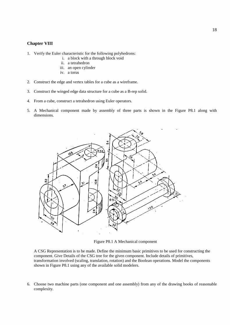
5. A Mechanical component made by assembly of three parts is shown in the Figure P8.1 along with

dimensions.

Figure P8.1 A Mechanical component

A CSG Representation is to be made. Define the minimum basic primitives to be used for constructing the component. Give Details of the CSG tree for the given component. Include details of primitives, transformation involved (scaling, translation, rotation) and the Boolean operations. Model the components shown in Figure P8.1 using any of the available solid modelers.

6. Choose two machine parts (one component and one assembly) from any of the drawing books of reasonable complexity.

19

i. Discuss the topological and geometrical aspects of the components in a coherent manner (point wise).

ii. Discuss steps to create the component by B-rep method. iii. Discuss steps to create the components by CSG. iv. Use any of the available solid modelers to create the components.

20

Chapter IX

1. Given a line A+td and a plane with base point B and normal vector n, what is the condition for the line to be perpendicular to the plane? What is the condition for the line to be parallel to the plane?

2. Find the proximity of the points (0, 0), (1, 5) and (1, 0) with respect to the line whose end points are A (1, 1) and B (1, 8).

3. Given n line segments in a plane, write an algorithm to answer the following query. For a point P, find the first line segment hit by a ray shot from the point towards right parallel to x-axis. (Hint: Find the point of intersection and order them in increasing magnitude of x.)

4. Consider the line segments whose end points are AB (0, 0) (5, 0); BC (5, 0) (5, 5); CD (5, 5) (0, 5) and DA (0, 5) (0, 0). Find the positioning of the point P (1, 1) with respect to these lines. Comment on the membership (inside/outside/on) of P in polygon ABCD.

5. A quadrilateral is represented by the vertices A (2, −2), B (0, 15), C (−2, −2) and D (0, 4). Determine if point E (0, −2) lies within this polygon. (Hint: For crossing test, the ray passes through the vertex A, thus infinitesimally shift the y coordinate of the ray and do the crossings test).

6. Given n points in a plane, devise an algorithm to construct a non self intersecting polygon. (Hint: Chose an extreme point and start connecting the immediate neighbors, keeping track of already connected vertices. There may be many possible solutions.)

7. Given a concave polygon and two points A and B inside the polygon, find the shortest path between the points. Consider all possibilities of how A and B are placed inside the polygon.

8. Consider a unit cube placed in the first octant of the coordinate frame. Find separately using the point in polyhedron algorithm the membership status of the points (−2, 0), (0.5, 5), (0.6, 0.8).

9. Consider a unit square placed in the first quadrant with two edges as the x and y axes. Also, consider an inscribing circle. Generate a quadtree data structure for the inscribed circle using the unit square as the root square. Generate to a depth of three levels. The quadtree thus generated can be used to find the membership of a point with respect to the circle. (Hint: Say for example a point is inside the circle, if it is inside/on any one of the node elements (squares) of the quadtree that are marked “in”. Thus, the computation of intersection reduces from ray tracing to searching the quadtree). Specifically, comment with the help of the quadtree representation of the circle about the placement of the points, (0.6, 0.6), (0.98, 0.98) and (2, 5). Also give the node number of the quadrant (e.g., Figure 9.15) in case the point is ‘inside’ the circle. Solve using graph paper.

10. Schematically, using the method presented in section 9.7, find the intersection (A *I B), union (A *

U B) and negation (A −* B) for the arrangements of polygons A and B as shown in Figures P9.1.

(a) (b) (c) (d)

Figure P9.1 Polygons A and B