Rotary Experiment #03: Speed Control - University of Hawaii · SRV02 Speed Control Laboratory – Student Manual 4.2. PI Control Design 4.2.1. Closed-loop Transfer Function The proportional-integral

Rotary Motion Servo Plant: SRV02

Rotary Experiment #03:Speed Control

SRV02 Speed Control using QuaRC

Student Manual

SRV02 Speed Control Laboratory – Student Manual

Table of Contents

1. INTRODUCTION..........................................................................................................................................1

2. PREREQUISITES.........................................................................................................................................1

3. OVERVIEW OF FILES..................................................................................................................................2

4. PRE-LAB ASSIGNMENTS.............................................................................................................................3

4.1. Desired Speed Control Response......................................................................................................34.1.1. SRV02 Speed Control Specifications.....................................................................................................3

4.1.2. Overshoot...............................................................................................................................................4

4.1.3. Steady-state Error...................................................................................................................................5

4.2. PI Control Design.............................................................................................................................74.2.1. Closed-loop Transfer Function...............................................................................................................7

4.2.2. Finding PI Gains to Satisfy Specifications.............................................................................................8

4.3. Lead Control Design.......................................................................................................................114.3.1. Finding Lead Compensator Parameters................................................................................................12

4.3.2. Magnitude Bode Plot of Uncompensated System................................................................................17

4.3.3. Phase Bode Plot of Uncompensated System........................................................................................20

4.4. Sensor Noise...................................................................................................................................22

5. IN-LAB PROCEDURES...............................................................................................................................24

5.1. Speed Control Simulation...............................................................................................................245.1.1. Setup for Speed Control Simulation.....................................................................................................24

5.1.2. Simulated PI Step Response.................................................................................................................25

5.1.3. Lead Compensator Design using Matlab .............................................................................................28

5.1.4. Simulated Lead Step Response............................................................................................................34

5.2. Speed Control Implementation.......................................................................................................365.2.1. Setup for Speed Control Implementation.............................................................................................37

Document Number 708 ♦ Revision 1.0 ♦ Page i


5.2.2. Implementation PI Speed Control........................................................................................................38

5.2.3. Implementation Lead Speed Control....................................................................................................41

5.3. Results Summary............................................................................................................................45

6. REFERENCES...........................................................................................................................................46

Document Number 708 ♦ Revision 1.0 ♦ Page ii


1. Introduction

The objective of this experiment is to develop a feedback system that controls the speed of the rotary servo load shaft. Both a proportional-integral (PI) controller and a lead compensator are designed to regulate the shaft speeds according to a set of specifications.

The following topics are covered in this laboratory: Design a proportional-integral (PI) controller that regulates the angular rate of the servo load

shaft according to certain time-domain requirements. Set-point weight. Design a lead compensator according to some time-domain and frequency-domain

specifications. Simulate the PI and lead controllers using the developed model of the plant and ensure the

specifications are met without any actuator saturation. Implement the controllers on the Quanser SRV02 device and evaluate its performance.

2. Prerequisites

In order to successfully carry out this laboratory, the user should be familiar with the following: Data acquisition card (e.g. Q8), the power amplifier (e.g. UPM), and the main components of

the SRV02 (e.g. actuator, sensors), as described in References [1], [4], and [5], respectively. Wiring and operating procedure of the SRV02 plant with the UPM and DAC device, as

discussed in Reference [5]. Transfer function fundamentals, e.g. obtaining a transfer function from a differential equation. Laboratory described in Reference [6] in order to be familiar using QuaRC with the SRV02.

Document Number 708 ♦ Revision 1.0 ♦ Page 1


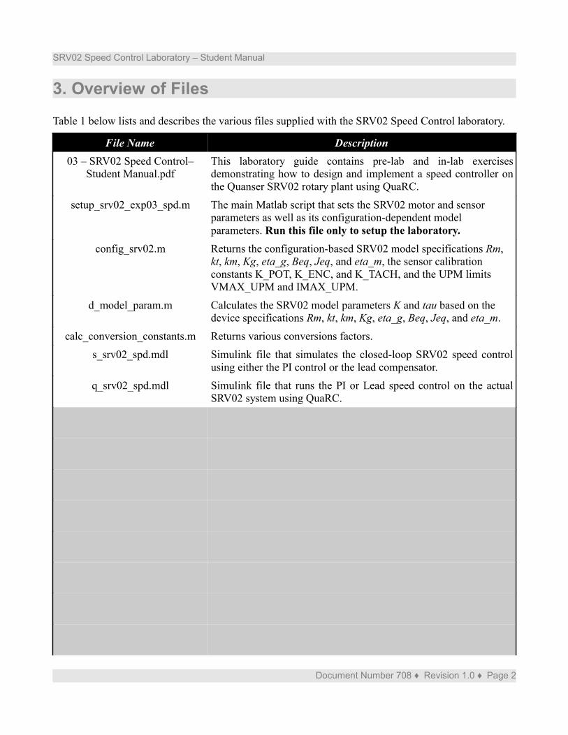
3. Overview of Files

Table 1 below lists and describes the various files supplied with the SRV02 Speed Control laboratory.

File Name Description03 – SRV02 Speed Control–

Student Manual.pdfThis laboratory guide contains pre-lab and in-lab exercises demonstrating how to design and implement a speed controller on the Quanser SRV02 rotary plant using QuaRC.

setup_srv02_exp03_spd.m The main Matlab script that sets the SRV02 motor and sensor parameters as well as its configuration-dependent model parameters. Run this file only to setup the laboratory.

config_srv02.m Returns the configuration-based SRV02 model specifications Rm, kt, km, Kg, eta_g, Beq, Jeq, and eta_m, the sensor calibration constants K_POT, K_ENC, and K_TACH, and the UPM limits VMAX_UPM and IMAX_UPM.

d_model_param.m Calculates the SRV02 model parameters K and tau based on the device specifications Rm, kt, km, Kg, eta_g, Beq, Jeq, and eta_m.

calc_conversion_constants.m Returns various conversions factors.

s_srv02_spd.mdl Simulink file that simulates the closed-loop SRV02 speed control using either the PI control or the lead compensator.

q_srv02_spd.mdl Simulink file that runs the PI or Lead speed control on the actual SRV02 system using QuaRC.



File Name Description

Table 1: Files supplied with the SRV02 Speed Control experiment.

4. Pre-Lab Assignments

4.1. Desired Speed Control ResponseSection 4.1.1 outlines the specifications of the closed-loop system. Given a step input with a certain amplitude, the expected overshoot and steady-state error of the system are calculated in Section 4.1.2 and Section 4.1.3, respectively.

4.1.1. SRV02 Speed Control SpecificationsThe time-domain requirements for controlling the speed of the SRV02 load shaft are:

= ess 0, [1]



≤ tp 0.05 [ ]s, and [2]

≤ PO 5 [ ]"%" . [3]

Thus when tracking the load shaft reference, the transient response should have a peak time less than or equal to 0.05 seconds, an overshoot less than or equal to 5 %, and zero steady-state error.

In addition to the above time-based specifications, the following frequency-domain requirements are to be met when designing the Lead compensator:

≤ 75.0 [ ]deg PM , and [4] = ω g 75.0 [ ]rad

. [5]

The phase margin mainly affects the shape of the response. Having a higher phase margin implies that the system is more stable and the corresponding time response will have less overshoot. The overshoot will not go beyond 5% with a phase margin of at least 75.0 degrees. The crossover frequency is the frequency where the gain of the bode plot is 1 (or 0 dB). This parameter mainly affects the speed of the response, thus having a larger ωg decreases the peak time. With a crossover frequency of 75.0 radians the resulting peak time will be less than or equal to 0.05 seconds.

4.1.2. OvershootConsider the following step setpoint

= ( )ω d t

2.5

rads

< t t0

7.5

rads

< t0 t,.

[6]

where t0 is the time the step is applied, i.e. step time. Initially the SRV02 should be running at 2.5 rad/s and after the step time it should jump up to 7.5 rad/s. Calculate the maximum overshoot of the response (in radians) when the step is applied.



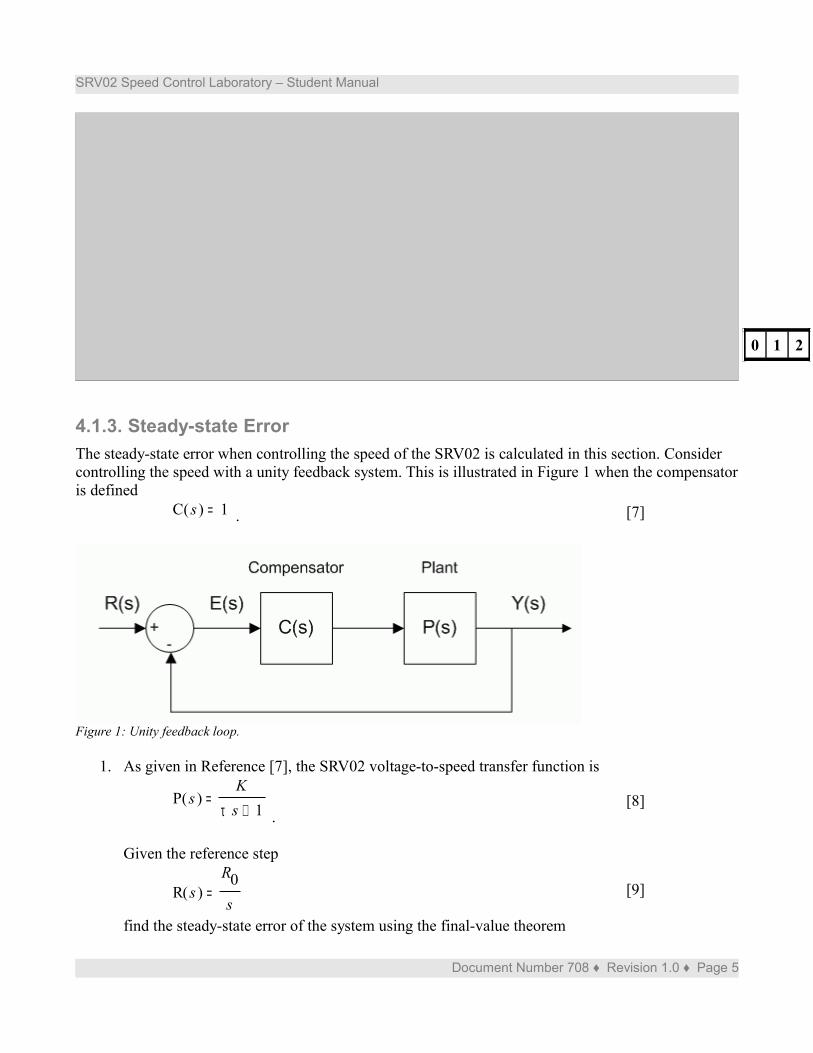
4.1.3. Steady-state ErrorThe steady-state error when controlling the speed of the SRV02 is calculated in this section. Consider controlling the speed with a unity feedback system. This is illustrated in Figure 1 when the compensator is defined

= ( )C s 1 . [7]

Figure 1: Unity feedback loop.

1. As given in Reference [7], the SRV02 voltage-to-speed transfer function is

= ( )P sK + τ s 1 .

[8]

Given the reference step

= ( )R sR0s

[9]

find the steady-state error of the system using the final-value theorem


0 1 2


= ess lim → s 0

s ( )E s

.[10]

Make sure the error transfer function E(s) derivation is shown.

2. Evaluate the steady-state error numerically based on the model parameters obtained in Reference [7] and the step amplitude R0 = 5.0 rad/s. Based on the steady-state error result from a step response with a unity proportional gain, what Type of system is the SRV02 when performing speed control (0, 1, 2, or 3)?


0 1 2


4.2. PI Control Design

4.2.1. Closed-loop Transfer FunctionThe proportional-integral (PI) compensator used to control the velocity of the SRV02 has the structure

= ( )Vm t − kp ( ) − bsp ( )ω d t ( )ω l t ki d⌠

⌡ − ( )ω d t ( )ω l t t [11]

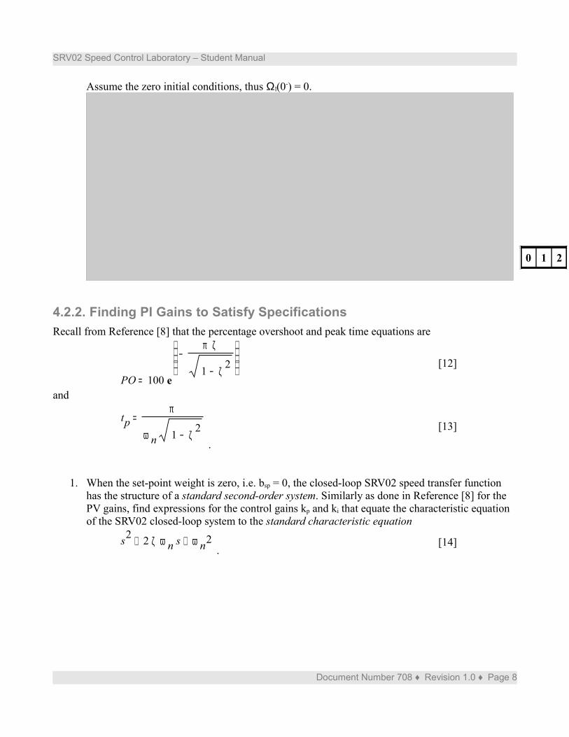
where kp is the proportional control gain, ki is the integral control gain, ωd(t) is the setpoint or reference load angular rate, ωl(t) is the measured load shaft angular rate, bsp is the set-point weight, and Vm(t) is the voltage applied to the SRV02 motor. The block diagram of the PI control is illustrated in Figure 2.

1. Find the closed-loop SRV02 speed transfer function, Ωl(s)/Ωd(s), using the time-based PI control defined in Equation [11], the block diagram in Figure 2, and the process model in [8].


0 1 2

Figure 2: Block diagram of SRV02 PI speed control.


Assume the zero initial conditions, thus Ωl(0-) = 0.

4.2.2. Finding PI Gains to Satisfy SpecificationsRecall from Reference [8] that the percentage overshoot and peak time equations are

= PO 100 e

−

π ζ

− 1 ζ2 [12]

and

= tpπ

ω n − 1 ζ2

.

[13]

1. When the set-point weight is zero, i.e. bsp = 0, the closed-loop SRV02 speed transfer function has the structure of a standard second-order system. Similarly as done in Reference [8] for the PV gains, find expressions for the control gains kp and ki that equate the characteristic equation of the SRV02 closed-loop system to the standard characteristic equation

+ + s2 2 ζ ω n s ω n2.

[14]


0 1 2


2. Compare the PI control gains needed to satisfy the speed control specifications with the PV gains found in Reference [8] to meet the position control requirements.


0 1 2


3. Calculate the minimum damping ratio and natural frequency required to meet the specifications given in Section 4.1.1.

4. Based on the nominal SRV02 model parameters, K and τ, found in Experiment #1: SRV02 Modeling (Reference [7]), calculate the PI control gains needed to satisfy the time-domain response requirements.


0 1 2

0 1 2


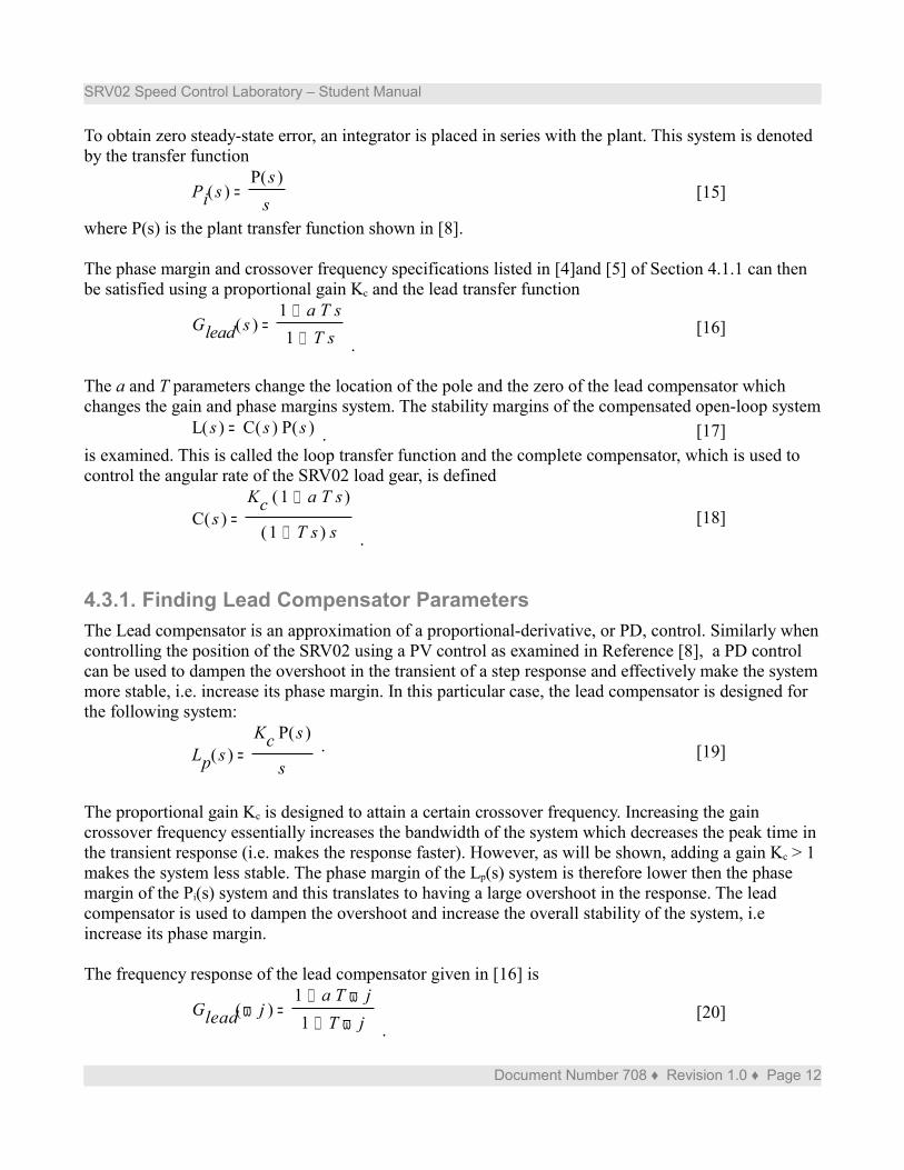
4.3. Lead Control DesignAlternatively, a lead or lag compensator can be designed to control the speed of the servo. The lag compensator is actually an approximation of a PI control and this, at first, may seem like the more viable option. However, due to the saturation limits of the actuator the lag compensator cannot achieve the desired zero steady-state error specification, which is given in [1] of Section 4.1.1. Instead a lead compensator with an integrator as shown in Figure 3 will be designed.

Figure 3: Closed-loop SRV02 speed control with lead compensator.


0 1 2


To obtain zero steady-state error, an integrator is placed in series with the plant. This system is denoted by the transfer function

= ( )Pi s( )P ss

[15]

where P(s) is the plant transfer function shown in [8].

The phase margin and crossover frequency specifications listed in [4]and [5] of Section 4.1.1 can then be satisfied using a proportional gain Kc and the lead transfer function

= ( )Glead s + 1 a T s

+ 1 T s .[16]

The a and T parameters change the location of the pole and the zero of the lead compensator which changes the gain and phase margins system. The stability margins of the compensated open-loop system

= ( )L s ( )C s ( )P s . [17]is examined. This is called the loop transfer function and the complete compensator, which is used to control the angular rate of the SRV02 load gear, is defined

= ( )C sKc ( ) + 1 a T s

( ) + 1 T s s .[18]

4.3.1. Finding Lead Compensator ParametersThe Lead compensator is an approximation of a proportional-derivative, or PD, control. Similarly when controlling the position of the SRV02 using a PV control as examined in Reference [8], a PD control can be used to dampen the overshoot in the transient of a step response and effectively make the system more stable, i.e. increase its phase margin. In this particular case, the lead compensator is designed for the following system:

= ( )Lp sKc ( )P s

s. [19]

The proportional gain Kc is designed to attain a certain crossover frequency. Increasing the gain crossover frequency essentially increases the bandwidth of the system which decreases the peak time in the transient response (i.e. makes the response faster). However, as will be shown, adding a gain Kc > 1 makes the system less stable. The phase margin of the Lp(s) system is therefore lower then the phase margin of the Pi(s) system and this translates to having a large overshoot in the response. The lead compensator is used to dampen the overshoot and increase the overall stability of the system, i.e increase its phase margin.

The frequency response of the lead compensator given in [16] is

= ( )Glead ω j + 1 a T ω j

+ 1 T ω j .[20]



and its corresponding magnitude and phase equations are

= ( )Glead ω j + T2 ω

2 a2 1

+ 1 T2 ω2

[20]

and = φ G − ( )arctan a T ω ( )arctan T ω

. [22]

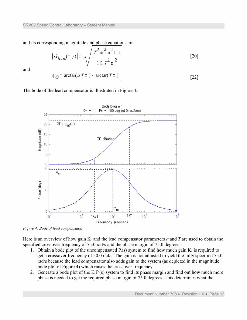
The bode of the lead compensator is illustrated in Figure 4.

Figure 4: Bode of lead compensator.

Here is an overview of how gain Kc and the lead compensator parameters a and T are used to obtain the specified crossover frequency of 75.0 rad/s and the phase margin of 75.0 degrees:

1. Obtain a bode plot of the uncompensated Pi(s) system to find how much gain Kc is required to get a crossover frequency of 50.0 rad/s. The gain is not adjusted to yield the fully specified 75.0 rad/s because the lead compensator also adds gain to the system (as depicted in the magnitude bode plot of Figure 4) which raises the crossover frequency.

2. Generate a bode plot of the KcPi(s) system to find its phase margin and find out how much more phase is needed to get the required phase margin of 75.0 degrees. This determines what the



maximum phase of the lead compensator, parameter φm, should be.3. Design a to get the necessary additional phase margin. The a parameter determines the

maximum phase of the lead compensator, φm, which is illustrated in Figure 4.4. Determine the frequency where the maximum phase of the lead compensator should occur,

shown in Figure 4 by the variable ωm.5. Calculate parameter T based on the values of a and ωm. 6. Obtain a bode of the open-loop compensated system, L(s) = C(s)P(s), and ensure the crossover

frequency and phase margin specifications are met.7. Simulate the step response and ensure the time-domain requirements are met.

The lead compensator has two parameters: a and T. To attain the maximum phase shown in Figure 4, φm, the Lead compensator has to add 20log10(a) of gain. This is determined using the equation

= a − + 1 ( )sin φ m

− + 1 ( )sin φ m .[23]

As illustrated in Figure 4, the maximum phase occurs at the maximum phase frequency ωm. Using the equation

= T1

ω m a,

[24]

parameter T is used to attain a certain maximum phase frequency. This changes where the Lead compensator breakpoint frequencies 1/(a*T) and 1/T shown in Figure 4 occur. The slope of the lead compensator gain changes at these frequencies.

1. Calculate how much gain, in dB, the lead compensator has to contribute in order for a system to get an additional phase margin of 45 degrees.

2. Find the breakpoint frequencies 1/(a*T) and 1/T needed for the maximum phase of the lead


0 1 2


compensator to occur at a frequency of 65.0 rad/s.

3. Show the derivation of Equation [24]. Thus show how to derive the frequency at which the maximum phase of the lead compensator occurs.


0 1 2

0 1 2


4. The maximum phase is defined by the expression = φ m − ( )arctan a T ω m ( )arctan T ω m . [25]

Using the derived maximum phase frequency and the trigonometric identity

= − ( )tan − + x y − ( )tan x ( )tan y

+ 1 ( )tan x ( )tan y[26]

show that the maximum phase equals

= ( )tan φ m − − a 1

2 a .[27]

5. Next, show how to derive the lead gain equation given in [23] from the exercises just completed and using the trigonometric identity

= ( )tan x( )sin x

− 1 ( )sin x 2.

[28]


0 1 2


4.3.2. Magnitude Bode Plot of Uncompensated SystemIn this section the bode plot of the Pi(s) system, i.e. the plant in series with an integrator, will be found.

1. Find the frequency response magnitude, |Pi(ω)|, of the transfer function Pi(s) given in [15].

2. The DC gain is the gain when the frequency is zero, i.e. ω = 0 rad/s. However, because of its integrator, Pi(s) has a singularity at zero frequency and the DC gain is therefore not technically defined for this system. Instead, approximate the DC gain by using ω = 1 rad/s. Make sure the DC gain estimate is evaluated numerically in dB using the nominal model parameters, K and τ, found in Reference [7].


0 1 2

0 1 2


3. The gain crossover frequency, ωg, is the frequency at which the gain of the system is 1 or 0 dB. Express the crossover frequency symbolically in terms of the SRV02 model parameters and then evaluate the expression using the nominal SRV02 model parameters.

4. Determine the breakpoints of |Pi(ω)|. Breakpoints are the asymptotes of the system which affect the slope of the magnitude plot. In this system there are two pole breakpoints that change the rate at which the gain is attenuated. Denote the higher-frequency breakpoint by the variable ωc.


0 1 2

0 1 2


5. Before drawing the bode magnitude plot, approximate the low-frequency gain of the system when ω < ωc and the high-frequency gain when ω > ωc. Breaking up the system into different frequency bands is especially useful when plotting the bode of more complex systems. Make sure the resulting equations are expressed in terms of the SRV02 model parameters and are also given in decibels.

6. Using the DC gain estimate, the gain crossover frequency, as well as the low and high-frequency gain approximations, draw the magnitude bode plot of the Pi(s) system. Label the bode plot with the DC gain along with the crossover and breakpoint frequencies.


0 1 2

0 1 2


4.3.3. Phase Bode Plot of Uncompensated SystemIn this section the phase bode plot of the uncompensated system will be plotted.

1. Find the phase of the Pi(s) system, φp(ω).


0 1 2


2. The phase margin is the amount of phase that is over -180 degrees when the gain is at 0 dB, i.e. at the gain crossover frequency. It is a way of determining relatively stability. The more phase margin, the more stable a system is and this translates to having less overshoot in the time-response of the system. Calculate the phase margin, PM, of the system.

3. Plot the phase bode of system Pi(s) and label where the gain crossover frequency occurs.


0 1 2

0 1 2


4.4. Sensor NoiseWhen using analog sensors such as a tachometer, there is often some inherent noise in the measured signal. In this section, the noise from the tachometer will be estimated.

1. The peak-to-peak noise of the measured SRV02 load gear signal can be calculated using

= eω1

100Kn ω l

,[29]

where Kn is the peak-to-peak ripple rating of the sensor and ωl is the speed of SRV02 load gear. Based on the ripple peak-to-peak specification of the tachometer given in Reference [5], calculate the amount of noise that is to be expected when the signal is running at 7.5 rad/s.


0 1 2


2. Taking the noise into account, what is the maximum peak in the speed response that is to be expected? Show the equation used and evaluate the peak value as well as the corresponding maximum percentage overshoot.


0 1 2

0 1 2


5. In-Lab Procedures

Students are asked to simulate the closed-loop PI and Lead responses. Then, the PI and Lead controllers are implemented on the actual SRV02. Before going through these experiments, go through Section 5.1.1 to configure the lab files according to your SRV02 setup.

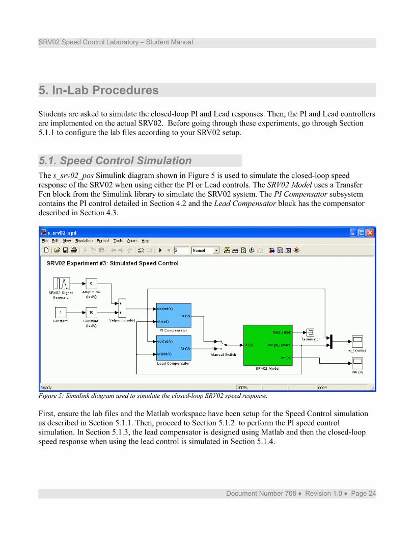
5.1. Speed Control SimulationThe s_srv02_pos Simulink diagram shown in Figure 5 is used to simulate the closed-loop speed response of the SRV02 when using either the PI or Lead controls. The SRV02 Model uses a Transfer Fcn block from the Simulink library to simulate the SRV02 system. The PI Compensator subsystem contains the PI control detailed in Section 4.2 and the Lead Compensator block has the compensator described in Section 4.3.

Figure 5: Simulink diagram used to simulate the closed-loop SRV02 speed response.

First, ensure the lab files and the Matlab workspace have been setup for the Speed Control simulation as described in Section 5.1.1. Then, proceed to Section 5.1.2 to perform the PI speed control simulation. In Section 5.1.3, the lead compensator is designed using Matlab and then the closed-loop speed response when using the lead control is simulated in Section 5.1.4.



5.1.1. Setup for Speed Control SimulationFollow these steps to configure the Matlab setup script and the Simulink diagram for the Speed Control simulation laboratory:

1. Load the Matlab software. 2. Browse through the Current Directory window in Matlab and find the folder that contains the

SRV02 speed controller files, e.g. s_srv02_spd.mdl. 3. Double-click on the s_srv02_spd.mdl file to open the SRV02 Speed Control Simulation

Simulink diagram shown in Figure 5.4. Double-click on the setup_srv02_exp03_spd.m file to open the setup script for the position

control Simulink models.5. Configure setup script: The controllers will be ran on an SRV02 in the high-gear configuration

with the disc load, as in Reference [7]. In order to simulate the SRV02 properly, make sure the script is setup to match this configuration, e.g. the EXT_GEAR_CONFIG should be set to 'HIGH' and the LOAD_TYPE should be set to 'DISC'. Also, ensure the ENCODER_TYPE, TACH_OPTION, K_CABLE, UPM_TYPE, and VMAX_DAC parameters are set according to the SRV02 system that is to be used in the laboratory. Next, set CONTROL_TYPE to 'MANUAL'.

6. Run the script by selecting the Debug | Run item from the menu bar or clicking on the Run button in the tool bar. The messages shown in Text 1, below, should be generated in the Matlab Command Window. The correct model parameters are loaded but the control gains and related parameters loaded are default values that need to be changed. That is, the PI control gains are all set to zero, the lead compensator parameters a and T are both set to 1, and the compensator proportional gain Kc is set to zero.

SRV02 model parameters: K = 1.53 rad/s/V tau = 0.0254 sPI control gains: kp = 0 V/rad ki = 0 V/rad/sLead compensator parameters: Kc = 0 V/rad/s 1/(a*T) = 1 rad/s 1/T = 1 rad/sText 1: Display message shown in Matlab Command Window after running setup_srv02_exp03_spd.m.

5.1.2. Simulated PI Step ResponseThe closed-loop step speed response of the SRV02 will be simulated to confirm that the designed PI control satisfies the specifications without saturating the motor. In addition, the affect of the set-point



weight will be examined.

Follow these steps to simulate the SRV02 PI speed response:1. Enter the proportional and integral control gains found in Section 4.2.2.

The speed reference signal is to be a 0.4 Hz square wave that goes between 2.5 rad/s and 7.5 rad/s (i.e. between 23.9 rpm and 71.6 rpm). In the SRV02 Signal Generator block, set the Signal Type to square and the Frequency to 0.4 Hz.

2. In the Speed Control Simulink model, set the Amplitude (rad/s) gain block to 2.5 rad/s and the Offset (rad/s) block to 5.0 rad/s.

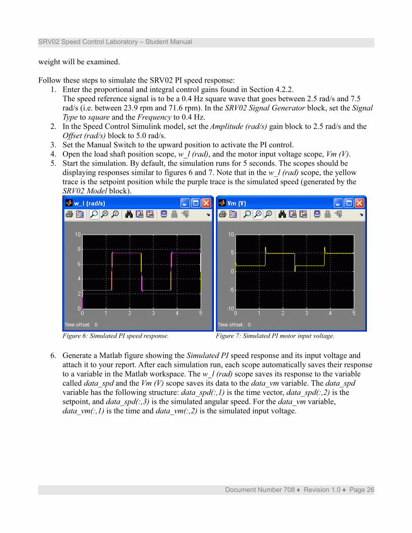
3. Set the Manual Switch to the upward position to activate the PI control.4. Open the load shaft position scope, w_l (rad), and the motor input voltage scope, Vm (V). 5. Start the simulation. By default, the simulation runs for 5 seconds. The scopes should be

displaying responses similar to figures 6 and 7. Note that in the w_l (rad) scope, the yellow trace is the setpoint position while the purple trace is the simulated speed (generated by the SRV02 Model block).

Figure 6: Simulated PI speed response. Figure 7: Simulated PI motor input voltage.

6. Generate a Matlab figure showing the Simulated PI speed response and its input voltage and attach it to your report. After each simulation run, each scope automatically saves their response to a variable in the Matlab workspace. The w_l (rad) scope saves its response to the variable called data_spd and the Vm (V) scope saves its data to the data_vm variable. The data_spd variable has the following structure: data_spd(:,1) is the time vector, data_spd(:,2) is the setpoint, and data_spd(:,3) is the simulated angular speed. For the data_vm variable, data_vm(:,1) is the time and data_vm(:,2) is the simulated input voltage.



7. Measure the steady-state error, the percentage overshoot, and the peak time of the simulated response. Does the response satisfy the specifications given in Section 4.1.1?


0 1 2


8. If the specifications are satisfied without overloading the servo motor, proceed to the next section to simulate the lead response.

5.1.3. Lead Compensator Design using Matlab In this section, Matlab is used to design a lead compensator that will satisfy the frequency-based specifications given in Section 4.1.1. Review the summarized design steps listed in Section 4.3.

Follow these steps to design the lead compensator for the SRV02 speed response:1. The bode plot of the open-loop uncompensated system, Pi(s), must first be found. This was

already done manually in Section 4.3 but Matlab will now be used. To generate the Bode of Pi(s), enter the following commands in Matlab:

% Plant transfer functionP = tf([K],[tau 1]);% Integrator transfer functionI = tf([1],[1 0]);% Plant with Integrator transfer functionPi = series(P,I);% Bode of Pi(s)figure(1)margin(Pi);set (1,'name','Pi(s)');

Recall that the model parameter K and tau are already stored in the Matlab workspace (after running the setup_srv02_exp03_spd.m script). These parameters are used with the commands tf and series to create the Pi(s) transfer function. The margin command generates a bode of the


0 1 2


system and it lists the gain and phase stability margins as well as the phase and gain crossover frequencies. Attach the bode to your report and compare it with the bode done manually in Section 4.3.

2. Find how more gain is required such that the gain crossover frequency is 50.0 rad/s (use the ginput Matlab command). As already mentioned, the lead compensator adds gain to the system and will increases the phase as well. Therefore gain Kc is not to be designed to meet the fully specified 75.0 rad/s. Generate a bode of the following loop transfer function Lp(s) defined in [19] to verify that the specified crossover frequency is achieved and attach it to your report. This also allows you to do any fine tuning to gain Kc.


0 1 2


3. Find the gain that the lead compensator needs to achieve the specified phase margin of 75 degrees. Give the amount in decibels. Also, to ensure the desired specifications are reached add another 5 degrees maximum phase of the lead.


0 1 2


4. The frequency at which the lead maximum phase occurs must be placed at the new gain crossover frequency ωg, new. This is the crossover frequency after the lead compensator is applied. As illustrated in Figure 4, ωm occurs halfway between 0 dB and 20Log10(a), i.e. at 10Log10(a). So the new gain crossover frequency in the Lp(s) system will be the frequency where the gain is -10Log10(a). Find this frequency and calculate what lead compensator breakpoint frequencies are needed.


0 1 2


5. Generate a bode of the lead compensator Clead(s), defined in [16].


0 1 2


6. Generate a bode of the loop transfer function L(s), as described in [17]. Does the phase margin and gain crossover frequency meet the specifications in Section 4.1.1?


0 1 2


7. Go on to Section 5.1.4 to simulate the step response and check whether the time-domain specifications are met. Keep it mind that the goal of the lead design is the same as the PI control, the response should meet the desired steady-state error, peak time, and percentage overshoot specifications given in Section 4.1.1. Thus if the crossover frequency and/or phase margin specifications are not quite satisfied, the response should be simulated to verify if the time-domain requirements are satisfied. If so, then the design is complete. If not, then the lead design needs to be re-visited.

5.1.4. Simulated Lead Step ResponseThe closed-loop step speed response of the SRV02 is simulated in order to verify that the time-based specifications in Section 4.1.1 are met without saturating the motor.


0 1 2


Follow these steps to simulate the SRV02 lead speed response:1. Enter the Kc, a, and T lead control parameters found in Section 5.1.3, above.2. In the SRV02 Signal Generator block, set the Signal Type to square and the Frequency to 0.4

Hz.3. In the Speed Control Simulink model, set the Amplitude (rad/s) gain block to 2.5 rad/s and the

Offset (rad/s) constant block to 5.0 rad/s.4. To engage the lead control, set the Manual Switch to the downward position.5. Open the load shaft position scope, w_l (rad), and the motor input voltage scope, Vm (V). 6. Start the simulation. By default, the simulation runs for 5 seconds. The scopes should be

displaying responses similar to figures 6 and 7.7. Verify if the time-domain specifications in Section 4.1.1 are satisfied and if the motor is being

saturated. To calculate the steady-state error, peak time, and percentage overshoot, use the simulated response data stored in the data_spd variable.

8. If the specifications are not satisfied, go back in the lead compensator design. You may have to, for example, need to add more maximum phase in order to increase the phase margin. If the specifications are met, move on to the next step.

9. Generate a Matlab figure showing the Simulated Lead speed response and its input voltage and attach it to your report.


0 1 2


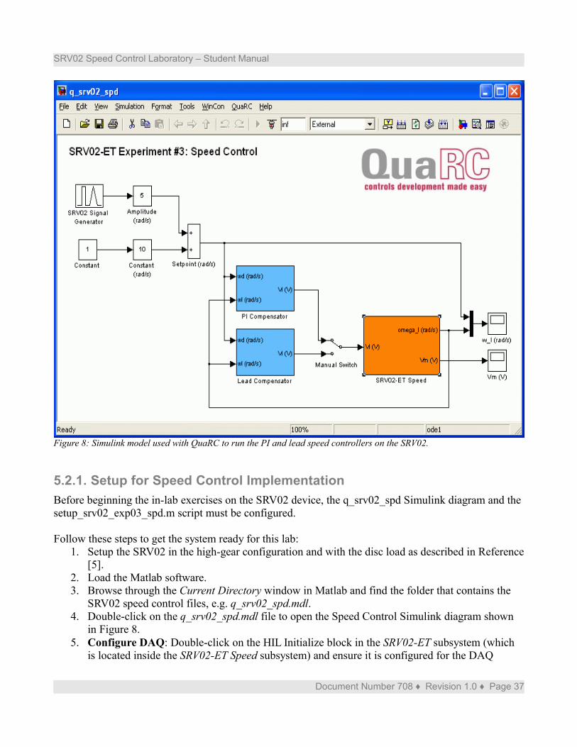
5.2. Speed Control ImplementationThe q_srv02_spd Simulink diagram shown in Figure 8 is used to perform the speed control exercises in this laboratory. The SRV02-ET Speed subsystem contains QuaRC blocks that interface with the DC motor and sensors of the SRV02 system, as discussed in Reference [6]. The PI Control subsystem implements the PI control detailed in Section 4.2 and the Lead Compensator block implements the lead control described in Section 4.3.


0 1 2


Figure 8: Simulink model used with QuaRC to run the PI and lead speed controllers on the SRV02.

5.2.1. Setup for Speed Control ImplementationBefore beginning the in-lab exercises on the SRV02 device, the q_srv02_spd Simulink diagram and the setup_srv02_exp03_spd.m script must be configured.

Follow these steps to get the system ready for this lab:1. Setup the SRV02 in the high-gear configuration and with the disc load as described in Reference

[5].2. Load the Matlab software.3. Browse through the Current Directory window in Matlab and find the folder that contains the

SRV02 speed control files, e.g. q_srv02_spd.mdl.4. Double-click on the q_srv02_spd.mdl file to open the Speed Control Simulink diagram shown

in Figure 8.5. Configure DAQ: Double-click on the HIL Initialize block in the SRV02-ET subsystem (which

is located inside the SRV02-ET Speed subsystem) and ensure it is configured for the DAQ



device that is installed in your system. See Reference [6] for more information on configuring the HIL Initialize block.

6. Configure Sensor: To perform the speed control experiment, the angular rate of the load shaft should be measured using the tachometer. This has already been set in the Spd Src Source block inside the SRV02-ET Speed subsystem.

7. Configure setup script: Set the parameters in the setup_srv02_exp03_spd.m script according to your system setup. See Section 5.1.1 for more details.

5.2.2. Implementation PI Speed ControlIn this lab, the angular rate of the SRV02 load shaft, i.e. the disc load, will be controlled using the developed PI control. Measurements will then be taken to ensure that the specifications are satisfied.

Follow the steps below:1. Run the setup_srv02_exp03_spd.m script.2. Enter the proportional and integral control gains found in Section 4.2.2.3. In the SRV02 Signal Generator block, set the Signal Type to square and the Frequency to 0.4


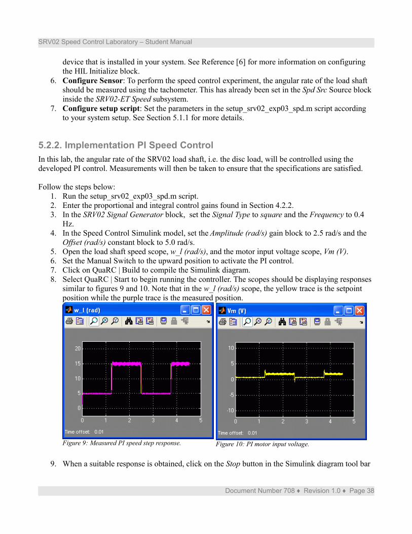
Offset (rad/s) constant block to 5.0 rad/s.5. Open the load shaft speed scope, w_l (rad/s), and the motor input voltage scope, Vm (V). 6. Set the Manual Switch to the upward position to activate the PI control.7. Click on QuaRC | Build to compile the Simulink diagram. 8. Select QuaRC | Start to begin running the controller. The scopes should be displaying responses

similar to figures 9 and 10. Note that in the w_l (rad/s) scope, the yellow trace is the setpoint position while the purple trace is the measured position.

Figure 9: Measured PI speed step response. Figure 10: PI motor input voltage.

9. When a suitable response is obtained, click on the Stop button in the Simulink diagram tool bar



(or select QuaRC | Stop from the menu) to stop running the code. Generate a Matlab figure showing the PI speed response and its input voltage. Attach it to your report. As in the s_srv02_spd Simulink diagram, when the controller is stopped each scope automatically saves their response to a variable in the Matlab workspace. Thus the theta_l (rad) scope saves its response to the data_spd variable and the Vm (V) scope saves its data to the data_vm variable.

10. Due to the noise in measured speed signal, it is difficult to obtain an accurate measurement of the specifications. In the Speed Control Simulink mode, set the Amplitude (rad) block to 0 rad/s and the Offset (rad) block to 7.5 rad/s in order to generate a constant speed reference of 7.5 rad/s. Generate a Matlab figure showing that illustrate the noise in the signal.


0 1 2


11. Measure the peak-to-peak ripple found in the speed signal, eω,meas, and compare it with the estimate in Section 4.4. Then, find the steady-state error by comparing the average of the measured signal with the desired speed. Is the steady-state error specification satisfied?


0 1 2


12. Measure the percentage overshoot and the peak time of the SRV02 load gear step response. Taking into account the noise in the signal, does the response satisfy the specifications given in Section 4.1.1?

13. Make sure QuaRC is stopped.14. Shut off the power of the UPM if no more experiments will be performed on the SRV02 in this

session.


0 1 2

0 1 2


5.2.3. Implementation Lead Speed ControlIn this section the speed of the SRV02 is controlled using the lead compensator. Measurements will then be taken to see if the specifications are satisfied.

Follow the steps below:1. Run the setup_srv02_exp03_spd.m script.2. Enter the Kc, a, and T, lead parameters found in Section 5.1.3.3. n the SRV02 Signal Generator block, set the Signal Type to square and the Frequency to 0.4


Offset (rad/s) constant block to 5.0 rad/s.5. To engage the lead compensator, set the Manual Switch in the Speed Control Simulink diagram

to the downward position.6. Open the load shaft speed scope, w_l (rad/s), and the motor input voltage scope, Vm (V). 7. Click on QuaRC | Build to compile the Simulink diagram. 8. Select QuaRC | Start to begin running the controller. The scopes should be displaying responses

similar to figures 9 and 10. 9. When a suitable response is obtained, click on the Stop button in the Simulink diagram tool bar

(or select QuaRC | Stop from the menu) to stop running the code. Generate a Matlab figure showing the lead speed response and its input voltage. Attach it to your report.



10. Measure the steady-state error, the percentage overshoot, and the peak time of the SRV02 load gear. For the steady-state error, it may be beneficial to give a constant reference and take its average as done in Section 5.2.2. Does the response satisfy the specifications given in Section 4.1.1?


0 1 2


11. Using both your simulation and implementation results, comment on any differences between the PI and lead controls.

12. Make sure QuaRC is stopped.13. Shut off the power of the UPM if no more experiments will be performed on the SRV02 in this

session.


0 1 2

0 1 2


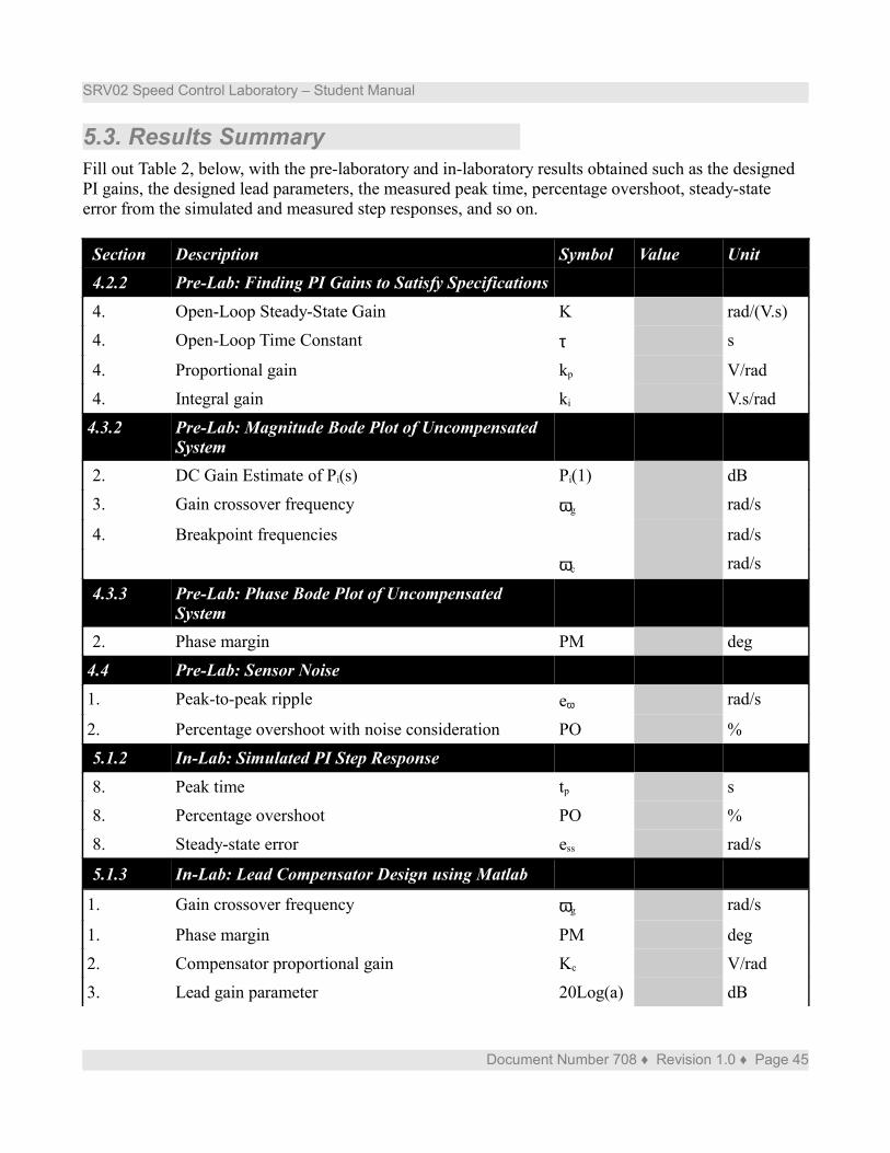
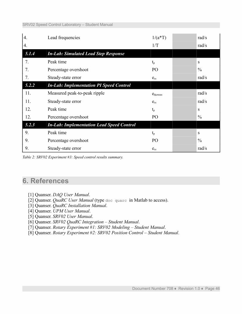
5.3. Results SummaryFill out Table 2, below, with the pre-laboratory and in-laboratory results obtained such as the designed PI gains, the designed lead parameters, the measured peak time, percentage overshoot, steady-state error from the simulated and measured step responses, and so on.

Section Description Symbol Value Unit4.2.2 Pre-Lab: Finding PI Gains to Satisfy Specifications4. Open-Loop Steady-State Gain K rad/(V.s)

4. Open-Loop Time Constant τ s

4. Proportional gain kp V/rad

4. Integral gain ki V.s/rad

4.3.2 Pre-Lab: Magnitude Bode Plot of UncompensatedSystem

2. DC Gain Estimate of Pi(s) Pi(1) dB

3. Gain crossover frequency ωg rad/s

4. Breakpoint frequencies rad/s

ωc rad/s

4.3.3 Pre-Lab: Phase Bode Plot of UncompensatedSystem

2. Phase margin PM deg

4.4 Pre-Lab: Sensor Noise1. Peak-to-peak ripple eω rad/s

2. Percentage overshoot with noise consideration PO %

5.1.2 In-Lab: Simulated PI Step Response8. Peak time tp s

8. Percentage overshoot PO %

8. Steady-state error ess rad/s

5.1.3 In-Lab: Lead Compensator Design using Matlab

1. Gain crossover frequency ωg rad/s

1. Phase margin PM deg

2. Compensator proportional gain Kc V/rad

3. Lead gain parameter 20Log(a) dB



4. Lead frequencies 1/(a*T) rad/s

4. 1/T rad/s

5.1.4 In-Lab: Simulated Lead Step Response

7. Peak time tp s



5.2.2 In-Lab: Implementation PI Speed Control11. Measured peak-to-peak ripple eω,meas rad/s


12. Peak time tp s


5.2.3 In-Lab: Implementation Lead Speed Control9. Peak time tp s



Table 2: SRV02 Experiment #3: Speed control results summary.

6. References

[1] Quanser. DAQ User Manual.[2] Quanser. QuaRC User Manual (type doc quarc in Matlab to access).[3] Quanser. QuaRC Installation Manual.[4] Quanser. UPM User Manual.[5] Quanser. SRV02 User Manual.[6] Quanser. SRV02 QuaRC Integration – Student Manual.[7] Quanser. Rotary Experiment #1: SRV02 Modeling – Student Manual.[8] Quanser. Rotary Experiment #2: SRV02 Position Control – Student Manual.


Documents

Rotary Experiment #03: Speed Control - University of Hawaii · SRV02 Speed Control Laboratory – Student Manual 4.2. PI Control Design 4.2.1. Closed-loop Transfer Function The proportional-integral