1

RONIN Technical Document for

DARPA Urban Challenge

Team AvantGuardium

May 31, 2007

Executive Summary

Team AvantGuardium was formed by US and Israeli defense R&D groups, who have been involved in the development and fielding of operational UGVs in real world applications. The team's vehicle Ronin is a Jeep Wrangler UGV. The autonomous vehicle concept relies on four principal subsystems that are optimally integrated and support each other. These 4 subsystems are:

• Inertial Navigation System (INS) • Vehicle Control System (VCM) • Obstacle Detection and avoidance Module (ODM) • Autonomous Decision-Making Module (ADM)

The vehicle is supported by a Path Finding Module (PFM) that computes a nominal route based on the route definition map and the mission file. Extensive fault detection system monitors the activities of all subsystems to ensure that each one is responding correctly to the environmental and vehicle situation and no conflicts between the systems occurs. The vehicle behavior is determined by an extensive set of rules. This set of rules is based on the interpretation of DARPA traffic rules and extensions that were added in order to respond to any situation that is conceived. The basic performance of the vehicle was evaluated by simulations, analyses and to some extends by field testing. DISCLAIMER: The information contained in this paper does not represent the official policies, either expressed or implied, of the Defense Advanced Research Projects Agency (DARPA) or the Department of Defense. DARPA does

not guarantee the accuracy or reliability of the information in this paper

2

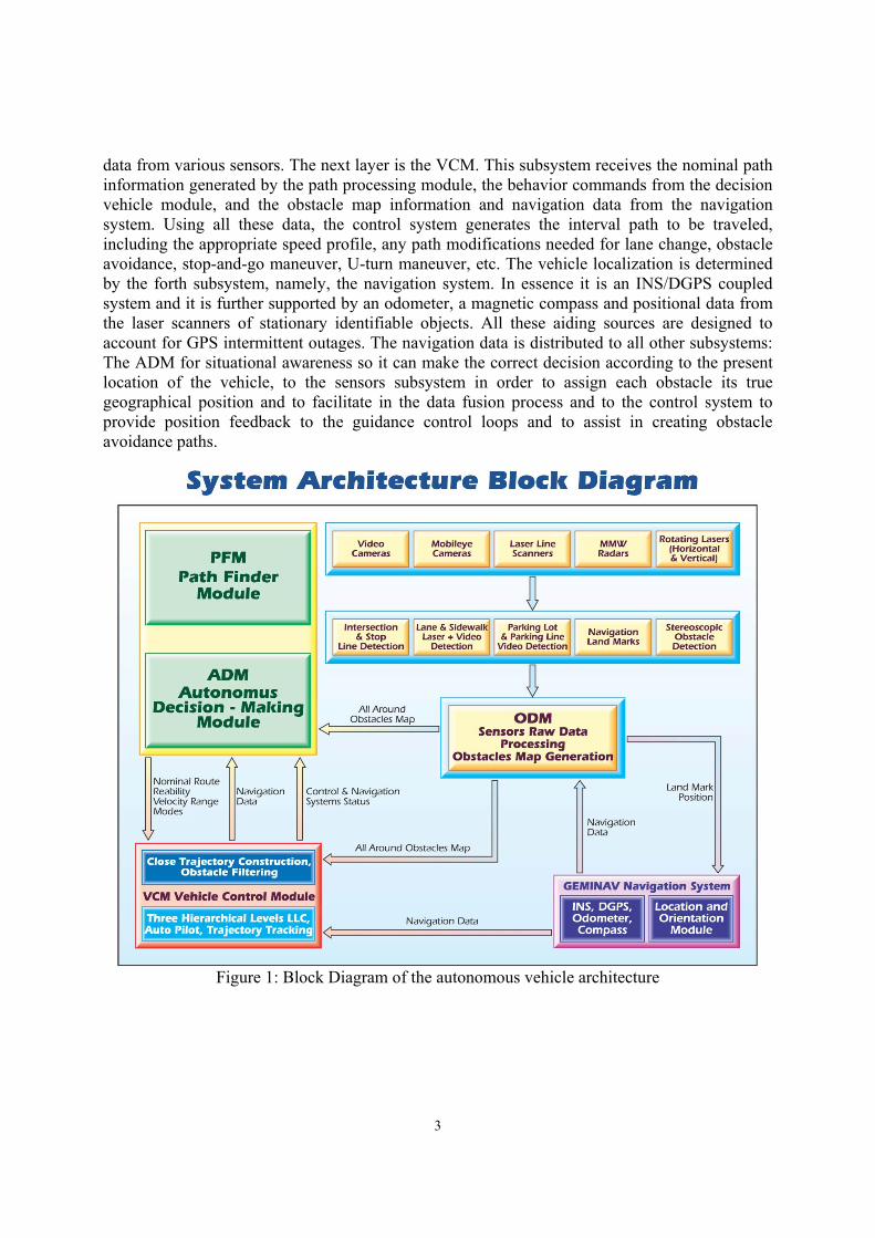
1. Introduction and Overview 1.1. Introduction Team AvantGuardium was formed by US and Israeli defense R&D groups, who have been involved in the development and fielding of operational UGVs in real world applications. The groups include EFW Inc., Elbit electro-optics ELOP, Elbit ground systems, MAFAT, and Ben-Gurion University. The group members are experienced engineers and scientists in the areas of robotics, control, electro-optics, computer vision, artificial intelligence, real-time software, system engineering and GIS. 1.2 Overall Problem Meeting the behavioral requirements of autonomous vehicles in the urban environment, as it is envisioned by DARPA and was set up as a test for the contenders, requires an enormous leap in the capabilities of the autonomous vehicle. Not only that the vehicle is required to precisely travel in narrow lanes, some of which are not clearly marked, using sparse and incomplete mapping information and intermittently perceptible GPS signal, but it also has to deal with highly dynamic environment that is manifested by many robots moving without human control each one with its own "mind", "mood" and "behavior". Although every robot is supposed to comply with certain well defined traffic and behavioral rules, the interpretation of these rules and their implementation in algorithms, software and sensors is highly uncertain and one should expect to encounter a highly stochastic "game" in which a large number of unpredictable robots interact with each other. This scenario dictates that the design of the autonomous vehicle should have a robust set of rules spanning, as many envisioned situations as possible and sound decision making logic. Any decision making system can only be as good as its source of information. In the case of the autonomous vehicle the sole source of information come from the vision sensors. 1.3 Team Approach AvantGuardium team's approach was to devote the design effort to four equally important elements: 1) vehicle control system; 2) navigation system; 3) obstacle detection and avoidance; 4) Rules supported event based Decision making. The team conviction is that a weak link in any one of these components will result in a failure of the complete system. To mitigate this risk a very powerful fault detection monitoring logic is part of the system. The role of the fault detection module is to detect any unexpected situation whether resulting from the dynamic response of the vehicle, or a suspicious navigational information, or unexpected obstacles information, then the system "interrogate" itself and based on set of rules it tries to determine the source of the fault, how to bypass the faulty element and what strategy to adopt so as to continue the mission. 1.4 System Architecture A block diagram showing the various subsystems and their interrelations is shown in Figure 1. The autonomous vehicle system, apart from the vehicle itself, is built around four main subsystems designed as authority layers. Data between the various subsystems flow through Ethernet communications using a hub. The first layer is the task management layer which includes the PFM, the ADM, data logging, vehicle management and mission data loader. The second layer includes the various environment sensors including the supporting processing computers that process the raw data to detect the obstacles and build an obstacle map by fusing

3

data from various sensors. The next layer is the VCM. This subsystem receives the nominal path information generated by the path processing module, the behavior commands from the decision vehicle module, and the obstacle map information and navigation data from the navigation system. Using all these data, the control system generates the interval path to be traveled, including the appropriate speed profile, any path modifications needed for lane change, obstacle avoidance, stop-and-go maneuver, U-turn maneuver, etc. The vehicle localization is determined by the forth subsystem, namely, the navigation system. In essence it is an INS/DGPS coupled system and it is further supported by an odometer, a magnetic compass and positional data from the laser scanners of stationary identifiable objects. All these aiding sources are designed to account for GPS intermittent outages. The navigation data is distributed to all other subsystems: The ADM for situational awareness so it can make the correct decision according to the present location of the vehicle, to the sensors subsystem in order to assign each obstacle its true geographical position and to facilitate in the data fusion process and to the control system to provide position feedback to the guidance control loops and to assist in creating obstacle avoidance paths.

Figure 1: Block Diagram of the autonomous vehicle architecture

4

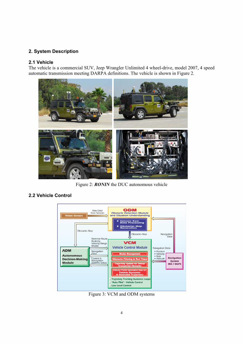
2. System Description 2.1 Vehicle The vehicle is a commercial SUV, Jeep Wrangler Unlimited 4 wheel-drive, model 2007, 4 speed automatic transmission meeting DARPA definitions. The vehicle is shown in Figure 2.

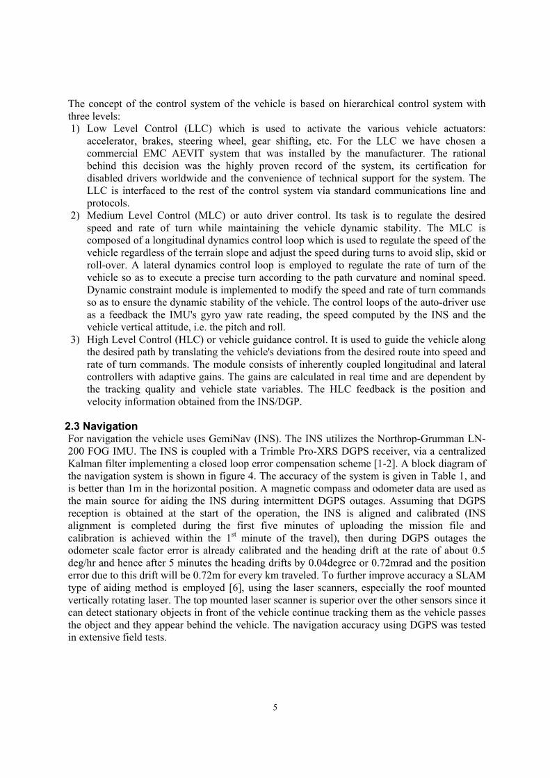
Figure 2: RONIN the DUC autonomous vehicle 2.2 Vehicle Control

Figure 3: VCM and ODM systems

5

The concept of the control system of the vehicle is based on hierarchical control system with three levels: 1) Low Level Control (LLC) which is used to activate the various vehicle actuators:

accelerator, brakes, steering wheel, gear shifting, etc. For the LLC we have chosen a commercial EMC AEVIT system that was installed by the manufacturer. The rational behind this decision was the highly proven record of the system, its certification for disabled drivers worldwide and the convenience of technical support for the system. The LLC is interfaced to the rest of the control system via standard communications line and protocols.

2) Medium Level Control (MLC) or auto driver control. Its task is to regulate the desired speed and rate of turn while maintaining the vehicle dynamic stability. The MLC is composed of a longitudinal dynamics control loop which is used to regulate the speed of the vehicle regardless of the terrain slope and adjust the speed during turns to avoid slip, skid or roll-over. A lateral dynamics control loop is employed to regulate the rate of turn of the vehicle so as to execute a precise turn according to the path curvature and nominal speed. Dynamic constraint module is implemented to modify the speed and rate of turn commands so as to ensure the dynamic stability of the vehicle. The control loops of the auto-driver use as a feedback the IMU's gyro yaw rate reading, the speed computed by the INS and the vehicle vertical attitude, i.e. the pitch and roll.

3) High Level Control (HLC) or vehicle guidance control. It is used to guide the vehicle along the desired path by translating the vehicle's deviations from the desired route into speed and rate of turn commands. The module consists of inherently coupled longitudinal and lateral controllers with adaptive gains. The gains are calculated in real time and are dependent by the tracking quality and vehicle state variables. The HLC feedback is the position and velocity information obtained from the INS/DGP.

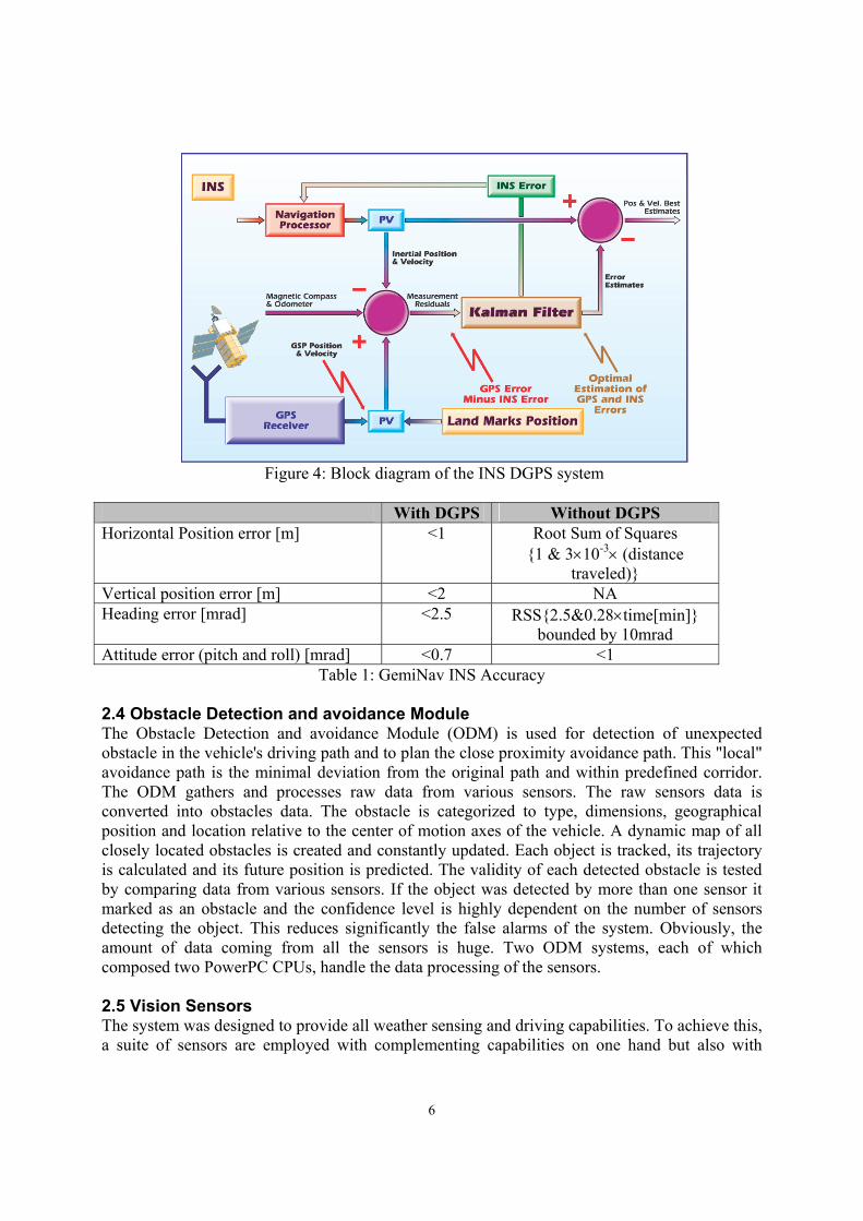
2.3 Navigation For navigation the vehicle uses GemiNav (INS). The INS utilizes the Northrop-Grumman LN-200 FOG IMU. The INS is coupled with a Trimble Pro-XRS DGPS receiver, via a centralized Kalman filter implementing a closed loop error compensation scheme [1-2]. A block diagram of the navigation system is shown in figure 4. The accuracy of the system is given in Table 1, and is better than 1m in the horizontal position. A magnetic compass and odometer data are used as the main source for aiding the INS during intermittent DGPS outages. Assuming that DGPS reception is obtained at the start of the operation, the INS is aligned and calibrated (INS alignment is completed during the first five minutes of uploading the mission file and calibration is achieved within the 1st minute of the travel), then during DGPS outages the odometer scale factor error is already calibrated and the heading drift at the rate of about 0.5 deg/hr and hence after 5 minutes the heading drifts by 0.04degree or 0.72mrad and the position error due to this drift will be 0.72m for every km traveled. To further improve accuracy a SLAM type of aiding method is employed [6], using the laser scanners, especially the roof mounted vertically rotating laser. The top mounted laser scanner is superior over the other sensors since it can detect stationary objects in front of the vehicle continue tracking them as the vehicle passes the object and they appear behind the vehicle. The navigation accuracy using DGPS was tested in extensive field tests.

6

Figure 4: Block diagram of the INS DGPS system

With DGPS Without DGPS Horizontal Position error [m] <1 Root Sum of Squares

{1 & 3×10-3× (distance traveled)}

Vertical position error [m] <2 NA Heading error [mrad] <2.5 RSS{2.5&0.28×time[min]}

bounded by 10mrad Attitude error (pitch and roll) [mrad] <0.7 <1

Table 1: GemiNav INS Accuracy 2.4 Obstacle Detection and avoidance Module The Obstacle Detection and avoidance Module (ODM) is used for detection of unexpected obstacle in the vehicle's driving path and to plan the close proximity avoidance path. This "local" avoidance path is the minimal deviation from the original path and within predefined corridor. The ODM gathers and processes raw data from various sensors. The raw sensors data is converted into obstacles data. The obstacle is categorized to type, dimensions, geographical position and location relative to the center of motion axes of the vehicle. A dynamic map of all closely located obstacles is created and constantly updated. Each object is tracked, its trajectory is calculated and its future position is predicted. The validity of each detected obstacle is tested by comparing data from various sensors. If the object was detected by more than one sensor it marked as an obstacle and the confidence level is highly dependent on the number of sensors detecting the object. This reduces significantly the false alarms of the system. Obviously, the amount of data coming from all the sensors is huge. Two ODM systems, each of which composed two PowerPC CPUs, handle the data processing of the sensors. 2.5 Vision Sensors The system was designed to provide all weather sensing and driving capabilities. To achieve this, a suite of sensors are employed with complementing capabilities on one hand but also with

7

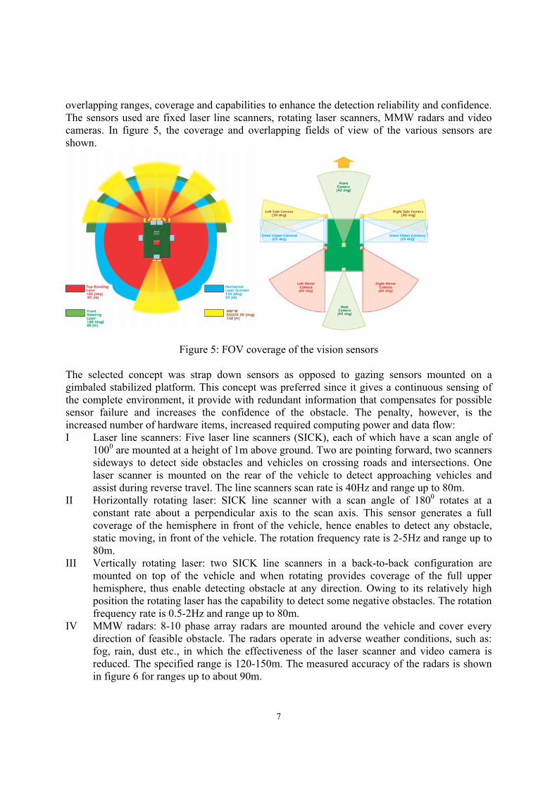
overlapping ranges, coverage and capabilities to enhance the detection reliability and confidence. The sensors used are fixed laser line scanners, rotating laser scanners, MMW radars and video cameras. In figure 5, the coverage and overlapping fields of view of the various sensors are shown.

Figure 5: FOV coverage of the vision sensors The selected concept was strap down sensors as opposed to gazing sensors mounted on a gimbaled stabilized platform. This concept was preferred since it gives a continuous sensing of the complete environment, it provide with redundant information that compensates for possible sensor failure and increases the confidence of the obstacle. The penalty, however, is the increased number of hardware items, increased required computing power and data flow: I Laser line scanners: Five laser line scanners (SICK), each of which have a scan angle of

1000 are mounted at a height of 1m above ground. Two are pointing forward, two scanners sideways to detect side obstacles and vehicles on crossing roads and intersections. One laser scanner is mounted on the rear of the vehicle to detect approaching vehicles and assist during reverse travel. The line scanners scan rate is 40Hz and range up to 80m.

II Horizontally rotating laser: SICK line scanner with a scan angle of 1800 rotates at a constant rate about a perpendicular axis to the scan axis. This sensor generates a full coverage of the hemisphere in front of the vehicle, hence enables to detect any obstacle, static moving, in front of the vehicle. The rotation frequency rate is 2-5Hz and range up to 80m.

III Vertically rotating laser: two SICK line scanners in a back-to-back configuration are mounted on top of the vehicle and when rotating provides coverage of the full upper hemisphere, thus enable detecting obstacle at any direction. Owing to its relatively high position the rotating laser has the capability to detect some negative obstacles. The rotation frequency rate is 0.5-2Hz and range up to 80m.

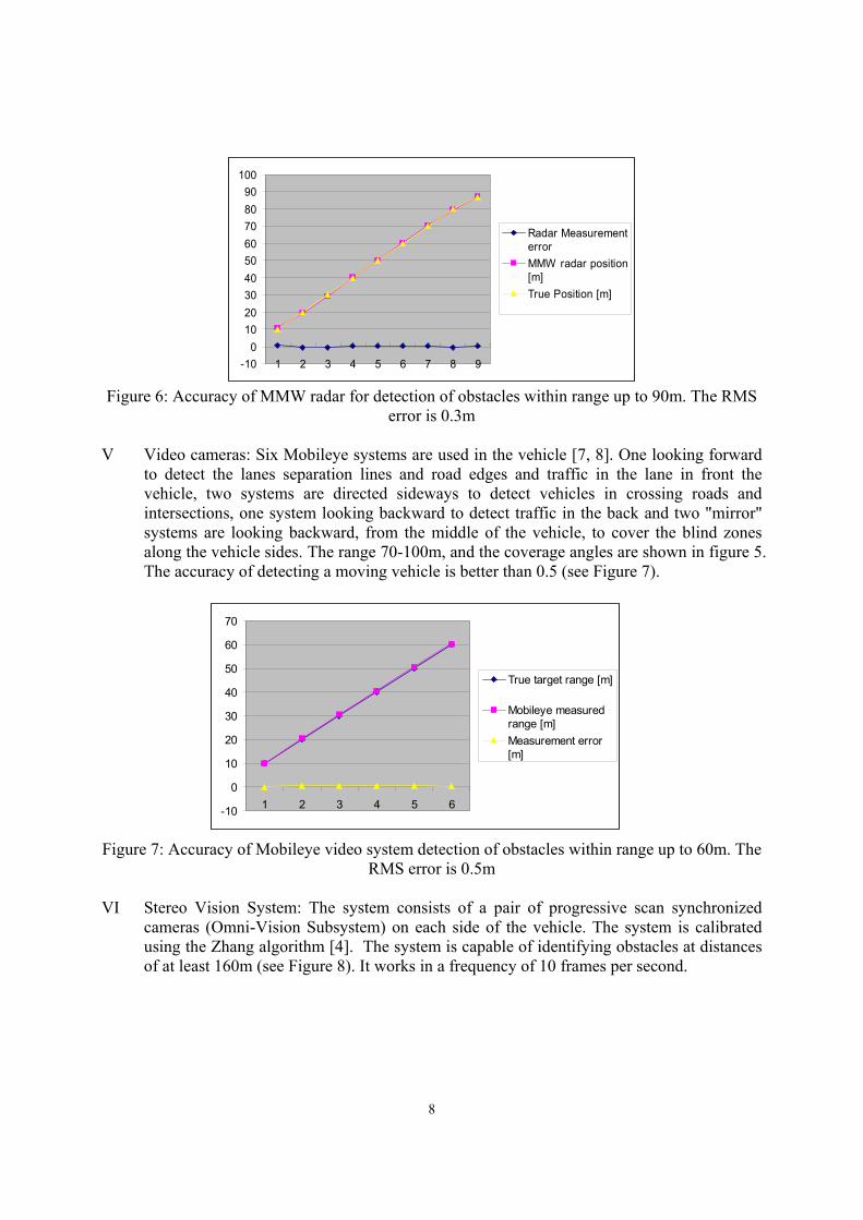
IV MMW radars: 8-10 phase array radars are mounted around the vehicle and cover every direction of feasible obstacle. The radars operate in adverse weather conditions, such as: fog, rain, dust etc., in which the effectiveness of the laser scanner and video camera is reduced. The specified range is 120-150m. The measured accuracy of the radars is shown in figure 6 for ranges up to about 90m.

8

-10

0

10

20

30

40

50

60

70

1 2 3 4 5 6

True target range [m]

Mobileye measuredrange [m]Measurement error[m]

-100

102030405060708090

100

1 2 3 4 5 6 7 8 9

Radar MeasurementerrorMMW radar position[m]True Position [m]

Figure 6: Accuracy of MMW radar for detection of obstacles within range up to 90m. The RMS

error is 0.3m

V Video cameras: Six Mobileye systems are used in the vehicle [7, 8]. One looking forward to detect the lanes separation lines and road edges and traffic in the lane in front the vehicle, two systems are directed sideways to detect vehicles in crossing roads and intersections, one system looking backward to detect traffic in the back and two "mirror" systems are looking backward, from the middle of the vehicle, to cover the blind zones along the vehicle sides. The range 70-100m, and the coverage angles are shown in figure 5. The accuracy of detecting a moving vehicle is better than 0.5 (see Figure 7).

Figure 7: Accuracy of Mobileye video system detection of obstacles within range up to 60m. The RMS error is 0.5m

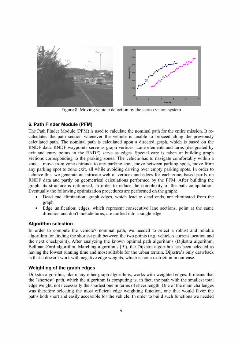
VI Stereo Vision System: The system consists of a pair of progressive scan synchronized

cameras (Omni-Vision Subsystem) on each side of the vehicle. The system is calibrated using the Zhang algorithm [4]. The system is capable of identifying obstacles at distances of at least 160m (see Figure 8). It works in a frequency of 10 frames per second.

9

Figure 8: Moving vehicle detection by the stereo vision system

6. Path Finder Module (PFM) The Path Finder Module (PFM) is used to calculate the nominal path for the entire mission. It re-calculates the path section whenever the vehicle is unable to proceed along the previously calculated path. The nominal path is calculated upon a directed graph, which is based on the RNDF data. RNDF waypoints serve as graph vertices. Lane elements and turns (designated by exit and entry points in the RNDF) serve as edges. Special care is taken of building graph sections corresponding to the parking zones. The vehicle has to navigate comfortably within a zone – move from zone entrance to any parking spot, move between parking spots, move from any parking spot to zone exit, all while avoiding driving over empty parking spots. In order to achieve this, we generate an intricate web of vertices and edges for each zone, based partly on RNDF data and partly on geometrical calculations performed by the PFM. After building the graph, its structure is optimized, in order to reduce the complexity of the path computation. Eventually the following optimization procedures are performed on the graph:

• Dead end elimination: graph edges, which lead to dead ends, are eliminated from the graph

• Edge unification: edges, which represent consecutive lane sections, point at the same direction and don't include turns, are unified into a single edge

Algorithm selection In order to compute the vehicle's nominal path, we needed to select a robust and reliable algorithm for finding the shortest path between the two points (e.g. vehicle's current location and the next checkpoint). After analyzing the known optimal path algorithms (Dijkstra algorithm, Bellman-Ford algorithm, Marching algorithms [9]), the Dijkstra algorithm has been selected as having the lowest running time and most suitable for the urban terrain. Dijkstra’s only drawback is that it doesn’t work with negative edge weights, which is not a restriction in our case.

Weighting of the graph edges Dijkstra algorithm, like many other graph algorithms, works with weighted edges. It means that the "shortest" path, which the algorithm is computing is, in fact, the path with the smallest total edge weight, not necessarily the shortest one in terms of sheer length. One of the main challenges was therefore selecting the most efficient edge weighting function, one that would favor the paths both short and easily accessible for the vehicle. In order to build such functions we needed

0

20

40

60

80

100

120

0 2 4 6 8 10

time (s)

dist

ance

(m)

10

to select the parameters, which would affect the weighting, and, by trial and error, assign appropriate coefficients to each parameter, each coefficient reflecting the relative importance of the parameter in the overall weight calculation.

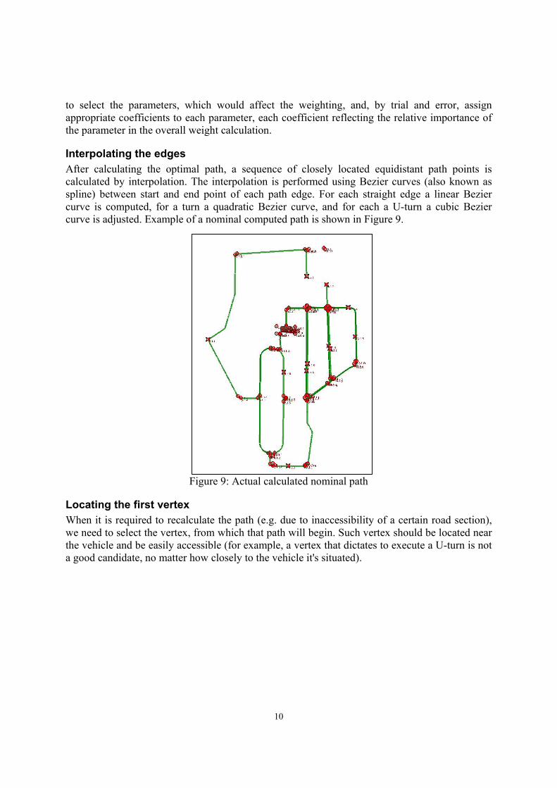
Interpolating the edges After calculating the optimal path, a sequence of closely located equidistant path points is calculated by interpolation. The interpolation is performed using Bezier curves (also known as spline) between start and end point of each path edge. For each straight edge a linear Bezier curve is computed, for a turn a quadratic Bezier curve, and for each a U-turn a cubic Bezier curve is adjusted. Example of a nominal computed path is shown in Figure 9.

Figure 9: Actual calculated nominal path

Locating the first vertex When it is required to recalculate the path (e.g. due to inaccessibility of a certain road section), we need to select the vertex, from which that path will begin. Such vertex should be located near the vehicle and be easily accessible (for example, a vertex that dictates to execute a U-turn is not a good candidate, no matter how closely to the vehicle it's situated).

11

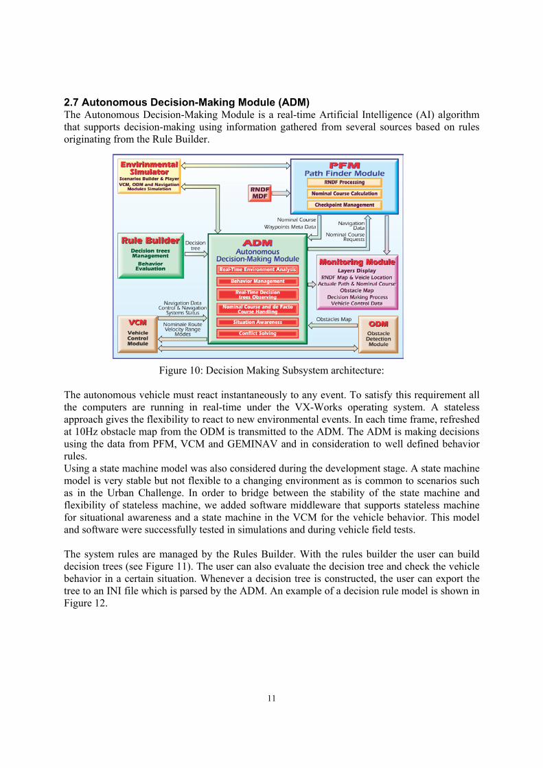
2.7 Autonomous Decision-Making Module (ADM) The Autonomous Decision-Making Module is a real-time Artificial Intelligence (AI) algorithm that supports decision-making using information gathered from several sources based on rules originating from the Rule Builder.

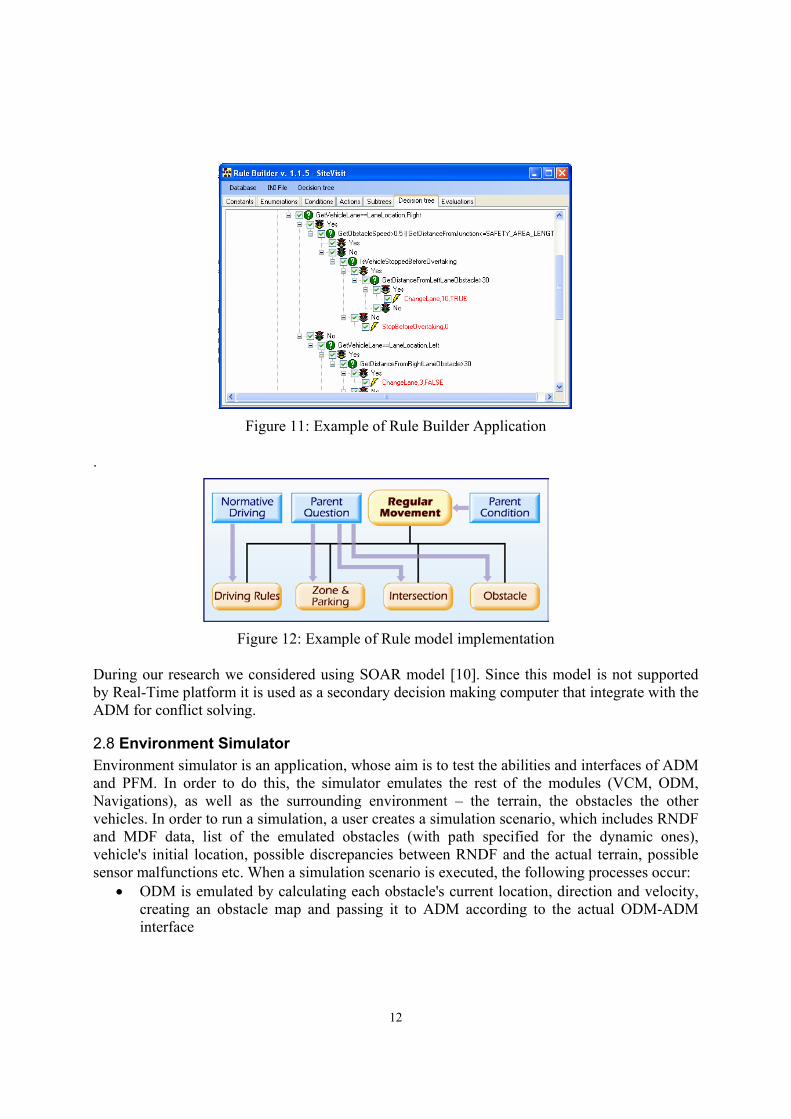
Figure 10: Decision Making Subsystem architecture: The autonomous vehicle must react instantaneously to any event. To satisfy this requirement all the computers are running in real-time under the VX-Works operating system. A stateless approach gives the flexibility to react to new environmental events. In each time frame, refreshed at 10Hz obstacle map from the ODM is transmitted to the ADM. The ADM is making decisions using the data from PFM, VCM and GEMINAV and in consideration to well defined behavior rules. Using a state machine model was also considered during the development stage. A state machine model is very stable but not flexible to a changing environment as is common to scenarios such as in the Urban Challenge. In order to bridge between the stability of the state machine and flexibility of stateless machine, we added software middleware that supports stateless machine for situational awareness and a state machine in the VCM for the vehicle behavior. This model and software were successfully tested in simulations and during vehicle field tests. The system rules are managed by the Rules Builder. With the rules builder the user can build decision trees (see Figure 11). The user can also evaluate the decision tree and check the vehicle behavior in a certain situation. Whenever a decision tree is constructed, the user can export the tree to an INI file which is parsed by the ADM. An example of a decision rule model is shown in Figure 12.

12

Figure 11: Example of Rule Builder Application

.

Figure 12: Example of Rule model implementation

During our research we considered using SOAR model [10]. Since this model is not supported by Real-Time platform it is used as a secondary decision making computer that integrate with the ADM for conflict solving.

2.8 Environment Simulator Environment simulator is an application, whose aim is to test the abilities and interfaces of ADM and PFM. In order to do this, the simulator emulates the rest of the modules (VCM, ODM, Navigations), as well as the surrounding environment – the terrain, the obstacles the other vehicles. In order to run a simulation, a user creates a simulation scenario, which includes RNDF and MDF data, list of the emulated obstacles (with path specified for the dynamic ones), vehicle's initial location, possible discrepancies between RNDF and the actual terrain, possible sensor malfunctions etc. When a simulation scenario is executed, the following processes occur:

• ODM is emulated by calculating each obstacle's current location, direction and velocity, creating an obstacle map and passing it to ADM according to the actual ODM-ADM interface

13

• VCM is emulated by accepting commands from ADM (according to the actual ADM-VCM interface) and moving the emulated vehicle, while using the same logic and tools as the real VCM.

• Navigation module is emulated by calculating the emulated vehicle's current location, direction and velocity (which are the product of the VCM emulation) and passing the data to the ADM, according to the actual Navigation-ADM interface

• The current simulation state (the RNDF-based map, the vehicle, the obstacles) is displayed on the screen in a user-friendly fashion

Thus we create a life-like environment for the ADM and PFM to operate within. ADM commands are generated based on the input data received from the emulated ODM and Navigation modules, exactly as they would be generated within the actual vehicle, allowing the developers to test the decision-making process.

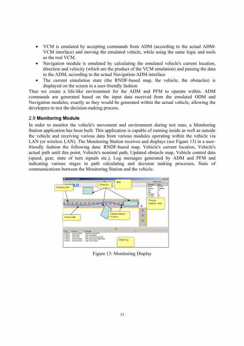
2.9 Monitoring Module In order to monitor the vehicle's movement and environment during test runs, a Monitoring Station application has been built. This application is capable of running inside as well as outside the vehicle and receiving various data from various modules operating within the vehicle via LAN (or wireless LAN). The Monitoring Station receives and displays (see Figure 13) in a user-friendly fashion the following data: RNDF-based map, Vehicle's current location, Vehicle's actual path until this point, Vehicle's nominal path, Updated obstacle map, Vehicle control data (speed, gear, state of turn signals etc.), Log messages generated by ADM and PFM and indicating various stages in path calculating and decision making processes, State of communications between the Monitoring Station and the vehicle.

Figure 13: Monitoring Display

14

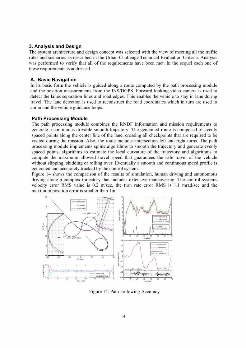
3. Analysis and Design The system architecture and design concept was selected with the view of meeting all the traffic rules and scenarios as described in the Urban Challenge Technical Evaluation Criteria. Analysis was performed to verify that all of the requirements have been met. In the sequel each one of these requirements is addressed. A. Basic Navigation In its basic form the vehicle is guided along a route computed by the path processing module and the position measurements from the INS/DGPS. Forward looking video camera is used to detect the lanes separation lines and road edges. This enables the vehicle to stay in lane during travel. The lane detection is used to reconstruct the road coordinates which in turn are used to command the vehicle guidance loops. Path Processing Module The path processing module combines the RNDF information and mission requirements to generate a continuous drivable smooth trajectory. The generated route is composed of evenly spaced points along the center line of the lane, crossing all checkpoints that are required to be visited during the mission. Also, the route includes intersection left and right turns. The path processing module implements spline algorithms to smooth the trajectory and generate evenly spaced points, algorithms to estimate the local curvature of the trajectory and algorithms to compute the maximum allowed travel speed that guarantees the safe travel of the vehicle without slipping, skidding or rolling over. Eventually a smooth and continuous speed profile is generated and accurately tracked by the control system. Figure 14 shows the comparison of the results of simulation, human driving and autonomous driving along a complex trajectory that includes extensive maneuvering. The control systems velocity error RMS value is 0.2 m/sec, the turn rate error RMS is 1.1 mrad/sec and the maximum position error is smaller than 1m.

Figure 14: Path Following Accuracy

15

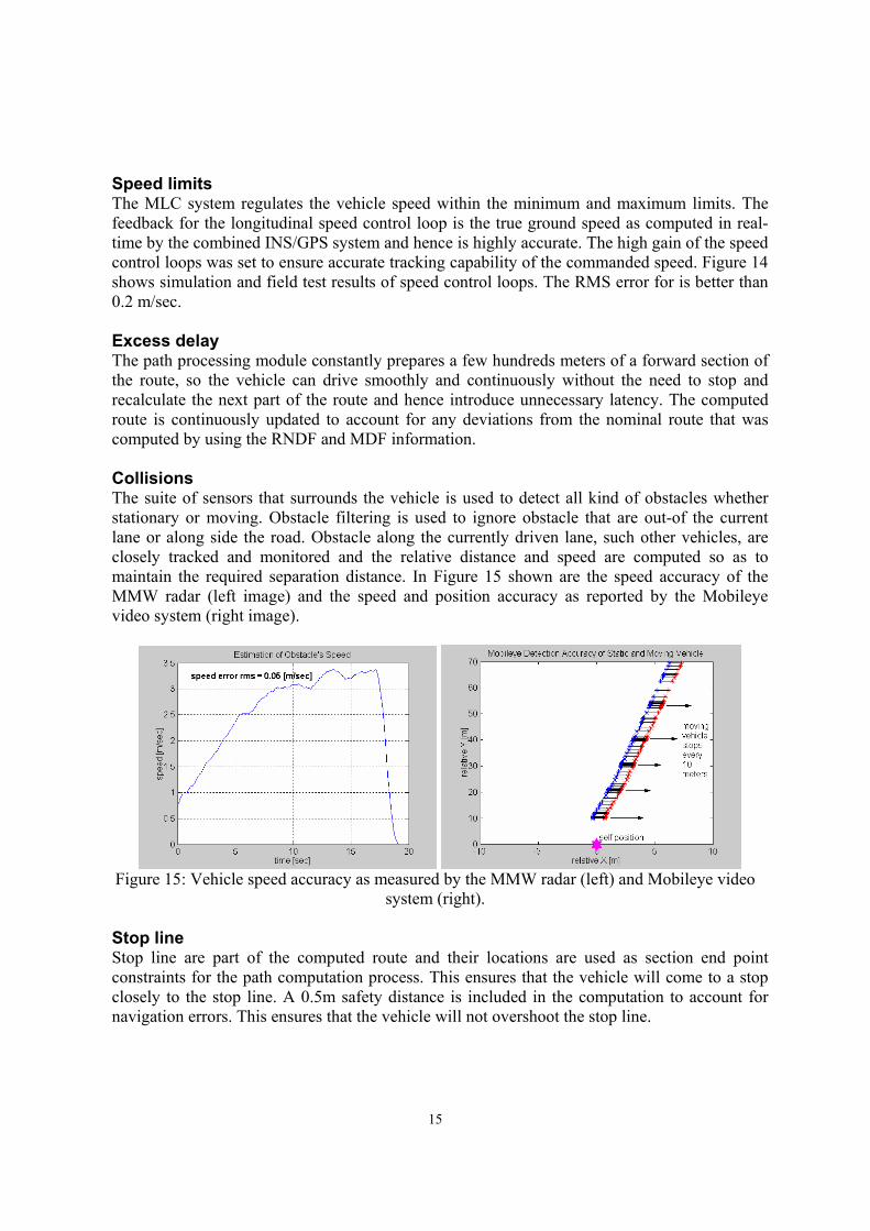
Speed limits The MLC system regulates the vehicle speed within the minimum and maximum limits. The feedback for the longitudinal speed control loop is the true ground speed as computed in real-time by the combined INS/GPS system and hence is highly accurate. The high gain of the speed control loops was set to ensure accurate tracking capability of the commanded speed. Figure 14 shows simulation and field test results of speed control loops. The RMS error for is better than 0.2 m/sec. Excess delay The path processing module constantly prepares a few hundreds meters of a forward section of the route, so the vehicle can drive smoothly and continuously without the need to stop and recalculate the next part of the route and hence introduce unnecessary latency. The computed route is continuously updated to account for any deviations from the nominal route that was computed by using the RNDF and MDF information. Collisions The suite of sensors that surrounds the vehicle is used to detect all kind of obstacles whether stationary or moving. Obstacle filtering is used to ignore obstacle that are out-of the current lane or along side the road. Obstacle along the currently driven lane, such other vehicles, are closely tracked and monitored and the relative distance and speed are computed so as to maintain the required separation distance. In Figure 15 shown are the speed accuracy of the MMW radar (left image) and the speed and position accuracy as reported by the Mobileye video system (right image).

Figure 15: Vehicle speed accuracy as measured by the MMW radar (left) and Mobileye video

system (right). Stop line Stop line are part of the computed route and their locations are used as section end point constraints for the path computation process. This ensures that the vehicle will come to a stop closely to the stop line. A 0.5m safety distance is included in the computation to account for navigation errors. This ensures that the vehicle will not overshoot the stop line.

16

Vehicle separation The obstacle detection sensors of the vehicle maintain tracking of all the vehicles in the vicinity. The vehicle's sensors provide measurements of the distance between the two vehicles. According to the speed of the vehicle the separation of one self vehicle length per 10mph speed is computed and the command is sent to the HLC loop which in turn modifies the speed command to the speed control loop in order to maintain a constant speed so as to maintain the desired separation distance. During stops and in safety areas the required distance of 1m sideways and back and 2m to the front, is ensured by imposing the separation distance as constraints for the path processing module and by continuously monitoring the obstacles distance to the vehicle. Leaving to pass and returning to lane Leaving a lane to pass a stopped vehicle require to detect the obstacle from a distance Ddet. In the case of double yellow line, this detection distance necessitate that the vehicle comes to a full stop at a distance that allows it to change lane with a separation equals to the vehicle length Lv. Since the vehicle length is Lv≈5m, and a moderate safe maneuver requires a distance of 2×Lv and the maximum stopping distance of the vehicle is 20m, the obstacle must be detected from a distance between 15m to 35m depending on the vehicle's speed, as given in Eq. (1).

)(3det vDLD stopv +×= (1) The returning maneuver is symmetric with the leaving maneuvers and hence equals to 3 time the vehicle length or 15m. In the case of a single yellow line the vehicle slows down to a safe maneuvering speed and performs the bypass with the same safety separation distance. In both cases the vehicle checks and verifies the clearance distance that ensures the safe completion of the detour. The testing involves detecting and measuring the closing velocities of approaching vehicles from both directions on the opposite lane. Obstacle detection Obstacle detection is achieved by using a suite of sensors that surround the vehicle and provide detection in all directions and ranges. Some sensors are overlapping to increase the probability of detection and confidence in detection. The coverage of each sensor is shown in Figure 5.

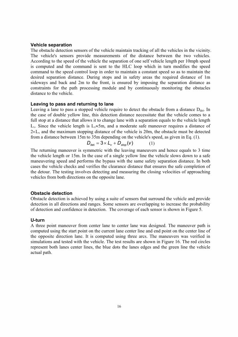
U-turn A three point maneuver from center lane to center lane was designed. The maneuver path is computed using the start point on the current lane center line and end point on the center line of the opposite direction lane. It is computed using three arcs. The maneuvers was verified in simulations and tested with the vehicle. The test results are shown in Figure 16. The red circles represent both lanes center lines, the blue dots the lanes edges and the green line the vehicle actual path.

17

Figure 16 U-turn maneuver testing

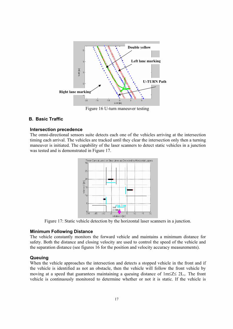
B. Basic Traffic Intersection precedence The omni-directional sensors suite detects each one of the vehicles arriving at the intersection timing each arrival. The vehicles are tracked until they clear the intersection only then a turning maneuver is initiated. The capability of the laser scanners to detect static vehicles in a junction was tested and is demonstrated in Figure 17.

Figure 17: Static vehicle detection by the horizontal laser scanners in a junction.

Minimum Following Distance The vehicle constantly monitors the forward vehicle and maintains a minimum distance for safety. Both the distance and closing velocity are used to control the speed of the vehicle and the separation distance (see figures 16 for the position and velocity accuracy measurements). Queuing When the vehicle approaches the intersection and detects a stopped vehicle in the front and if the vehicle is identified as not an obstacle, then the vehicle will follow the front vehicle by moving at a speed that guarantees maintaining a queuing distance of 1m≤Z≤ 2Lv. The front vehicle is continuously monitored to determine whether or not it is static. If the vehicle is

Right lane marking

Left lane marking

Double yellow

U-TURN Path

18

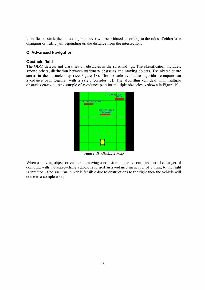
identified as static then a passing maneuver will be initiated according to the rules of either lane changing or traffic jam depending on the distance from the intersection. C. Advanced Navigation Obstacle field The ODM detects and classifies all obstacles in the surroundings. The classification includes, among others, distinction between stationary obstacles and moving objects. The obstacles are stored in the obstacle map (see Figure 18). The obstacle avoidance algorithm computes an avoidance path together with a safety corridor [3]. The algorithm can deal with multiple obstacles en-route. An example of avoidance path for multiple obstacles is shown in Figure 19.

Figure 18: Obstacle Map

When a moving object or vehicle is moving a collision course is computed and if a danger of colliding with the approaching vehicle is sensed an avoidance maneuver of pulling to the right is initiated. If no such maneuver is feasible due to obstructions to the right then the vehicle will come to a complete stop.

19

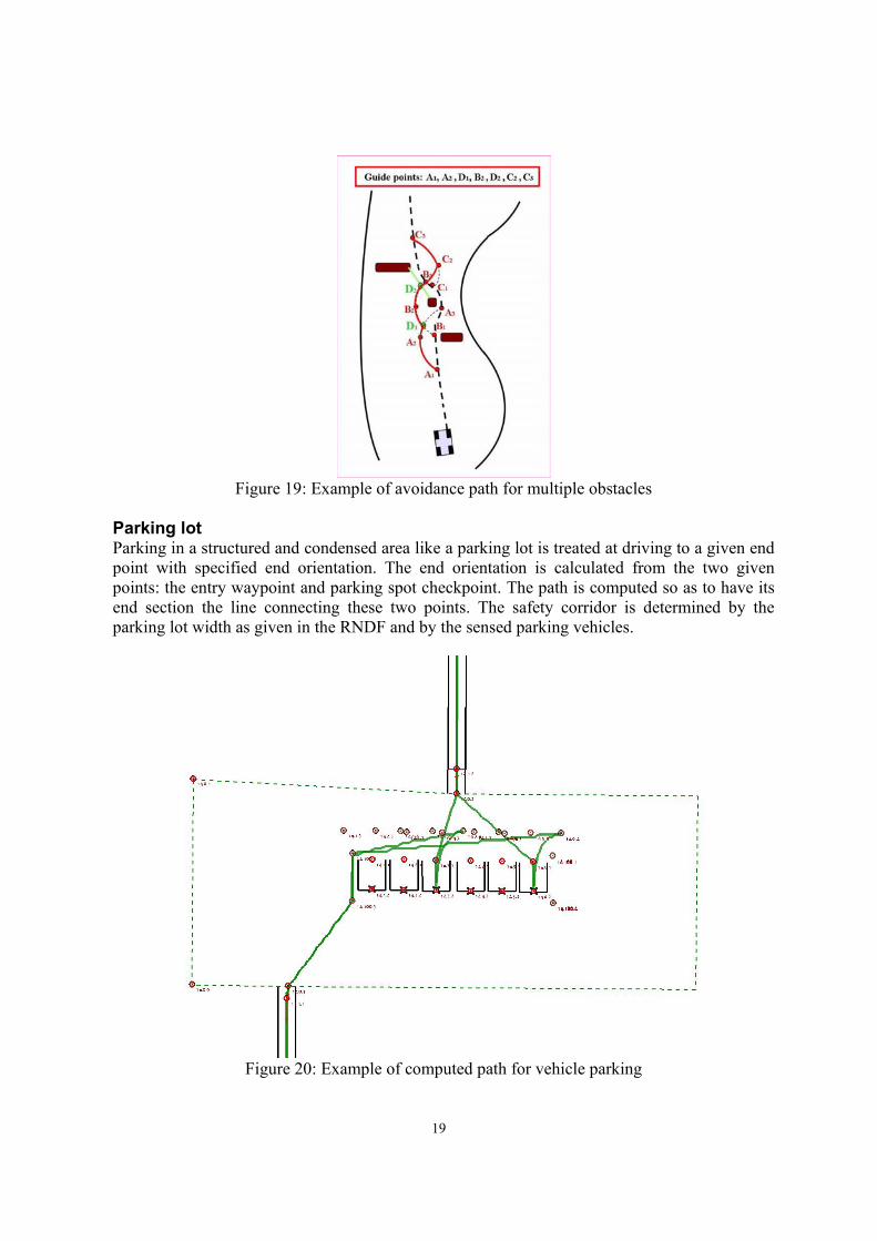
Figure 19: Example of avoidance path for multiple obstacles

Parking lot Parking in a structured and condensed area like a parking lot is treated at driving to a given end point with specified end orientation. The end orientation is calculated from the two given points: the entry waypoint and parking spot checkpoint. The path is computed so as to have its end section the line connecting these two points. The safety corridor is determined by the parking lot width as given in the RNDF and by the sensed parking vehicles.

Figure 20: Example of computed path for vehicle parking

20

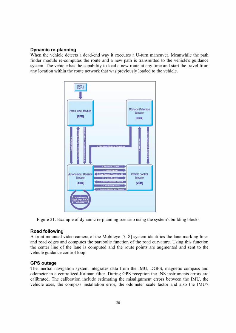
Dynamic re-planning When the vehicle detects a dead-end way it executes a U-turn maneuver. Meanwhile the path finder module re-computes the route and a new path is transmitted to the vehicle's guidance system. The vehicle has the capability to load a new route at any time and start the travel from any location within the route network that was previously loaded to the vehicle.

Figure 21: Example of dynamic re-planning scenario using the system's building blocks Road following A front mounted video camera of the Mobileye [7, 8] system identifies the lane marking lines and road edges and computes the parabolic function of the road curvature. Using this function the center line of the lane is computed and the route points are augmented and sent to the vehicle guidance control loop. GPS outage The inertial navigation system integrates data from the IMU, DGPS, magnetic compass and odometer in a centralized Kalman filter. During GPS reception the INS instruments errors are calibrated. The calibration include estimating the misalignment errors between the IMU, the vehicle axes, the compass installation error, the odometer scale factor and also the IMU's

21

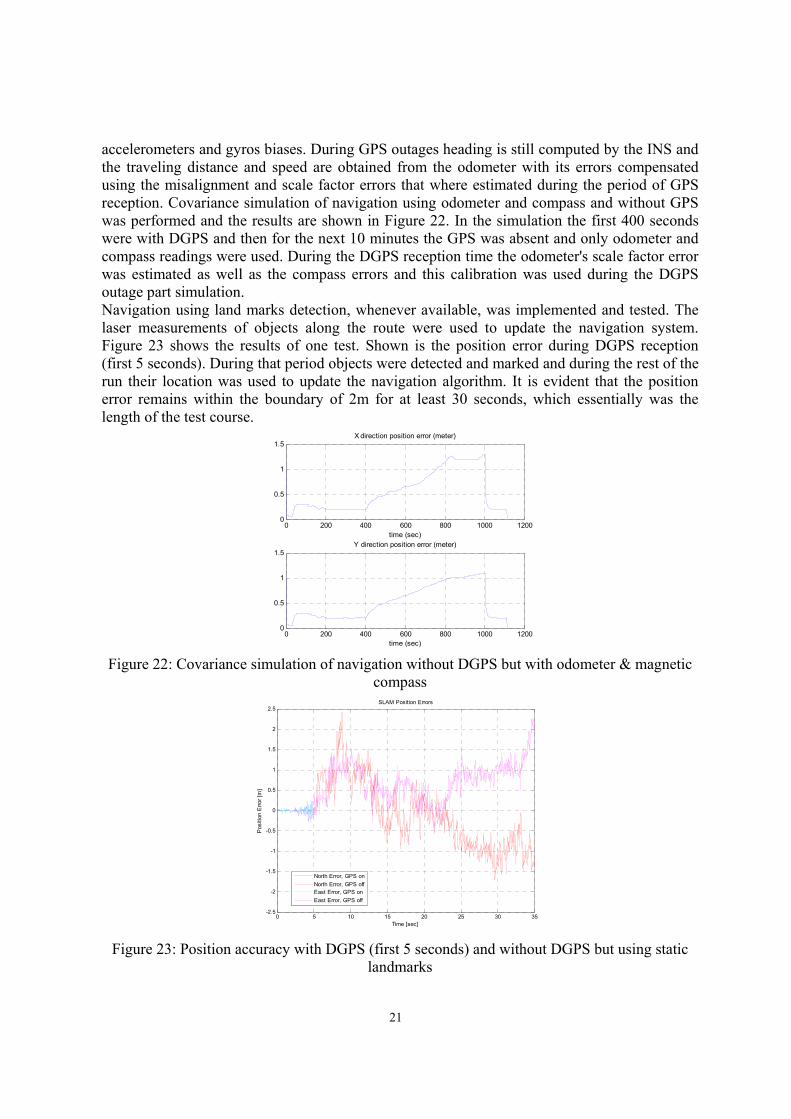
accelerometers and gyros biases. During GPS outages heading is still computed by the INS and the traveling distance and speed are obtained from the odometer with its errors compensated using the misalignment and scale factor errors that where estimated during the period of GPS reception. Covariance simulation of navigation using odometer and compass and without GPS was performed and the results are shown in Figure 22. In the simulation the first 400 seconds were with DGPS and then for the next 10 minutes the GPS was absent and only odometer and compass readings were used. During the DGPS reception time the odometer's scale factor error was estimated as well as the compass errors and this calibration was used during the DGPS outage part simulation. Navigation using land marks detection, whenever available, was implemented and tested. The laser measurements of objects along the route were used to update the navigation system. Figure 23 shows the results of one test. Shown is the position error during DGPS reception (first 5 seconds). During that period objects were detected and marked and during the rest of the run their location was used to update the navigation algorithm. It is evident that the position error remains within the boundary of 2m for at least 30 seconds, which essentially was the length of the test course.

0 200 400 600 800 1000 12000

0.5

1

1.5X direction position error (meter)

time (sec)

0 200 400 600 800 1000 12000

0.5

1

1.5Y direction position error (meter)

time (sec) Figure 22: Covariance simulation of navigation without DGPS but with odometer & magnetic

compass

0 5 10 15 20 25 30 35-2.5

-2

-1.5

-1

-0.5

0

0.5

1

1.5

2

2.5

Time [sec]

Pos

ition

Erro

r [m

]

SLAM Position Errors

North Error, GPS onNorth Error, GPS offEast Error, GPS onEast Error, GPS off

Figure 23: Position accuracy with DGPS (first 5 seconds) and without DGPS but using static

landmarks

22

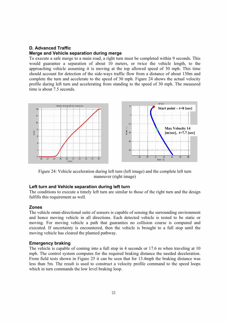
D. Advanced Traffic Merge and Vehicle separation during merge To execute a safe merge to a main road, a right turn must be completed within 9 seconds. This would guarantee a separation of about 10 meters, or twice the vehicle length, to the approaching vehicle assuming it is moving at the top allowed speed of 30 mph. This time should account for detection of the side-ways traffic flow from a distance of about 130m and complete the turn and accelerate to the speed of 30 mph. Figure 24 shows the actual velocity profile during left turn and accelerating from standing to the speed of 30 mph. The measured time is about 7.5 seconds.

Figure 24: Vehicle acceleration during left turn (left image) and the complete left turn

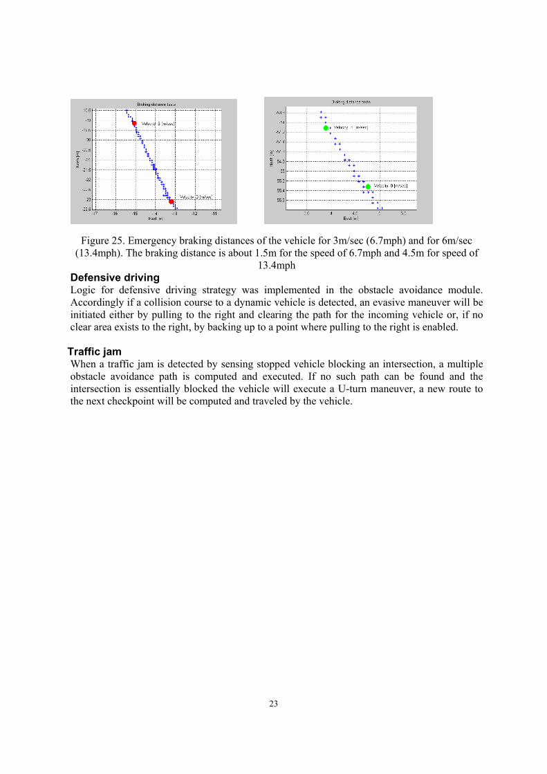
maneuver (right image) Left turn and Vehicle separation during left turn The conditions to execute a timely left turn are similar to those of the right turn and the design fulfills this requirement as well. Zones The vehicle omni-directional suite of sensors is capable of sensing the surrounding environment and hence moving vehicle in all directions. Each detected vehicle is tested to be static or moving. For moving vehicle a path that guaranties no collision course is computed and executed. If uncertainty is encountered, then the vehicle is brought to a full stop until the moving vehicle has cleared the planned pathway. Emergency braking The vehicle is capable of coming into a full stop in 4 seconds or 17.6 m when traveling at 10 mph. The control system computes for the required braking distance the needed deceleration. From field tests shown in Figure 25 it can be seen that for 13.4mph the braking distance was less than 5m. The result is used to construct a velocity profile command to the speed loops which in turn commands the low level braking loop.

Start point – t=0 [sec]

Max Velocity 14 [m/sec], t=7.7 [sec]

23

Figure 25. Emergency braking distances of the vehicle for 3m/sec (6.7mph) and for 6m/sec (13.4mph). The braking distance is about 1.5m for the speed of 6.7mph and 4.5m for speed of

13.4mph Defensive driving Logic for defensive driving strategy was implemented in the obstacle avoidance module. Accordingly if a collision course to a dynamic vehicle is detected, an evasive maneuver will be initiated either by pulling to the right and clearing the path for the incoming vehicle or, if no clear area exists to the right, by backing up to a point where pulling to the right is enabled.

Traffic jam When a traffic jam is detected by sensing stopped vehicle blocking an intersection, a multiple obstacle avoidance path is computed and executed. If no such path can be found and the intersection is essentially blocked the vehicle will execute a U-turn maneuver, a new route to the next checkpoint will be computed and traveled by the vehicle.

24

References 1. Greenspan, R.L., GPS and Inertial Integration, in: Parkinson, B.W. and Spilker, J.J., (eds.),

Global Positioning System: Theory and Applications (Vol. II), American Institute of Astronautics and Aeronautics, 1996.

2. Grewal, M.S., Weill, L.R. and Andrews, A.P., Global Positioning Systems, Inertial Navigation, and Integration, John Wiley and Sons, New York, 2001.

3. Shmaglit, A., Rinat, K., Brand, Z., Fischler, A. and Velger M., "Autonomous Vehicle Control and Obstacle Avoidance Concepts Oriented to Meet the Challenging Requirements of Realistic Missions", Proceedings of the 9th International Conference on Control, Automation, Robotics and Vision, Singapore, December 2006.

4. Shmaglit, A., Rinat, K., Brand, Z., Fischler, A. and Velger M., "Incorporation of Obstacle Avoidance Into Autonomous Path Following with Emphasis on Dynamic Stability and High Real-Time Performance", Presented at the AEAI workshop on advances in robotics, Tel-Aviv University, 2006.

5. Zhang, "A Flexible New Technique for Camera Calibration", IEEE transactions on pattern analysis and machine intelligence, 22(11):1330-1334, November 2000.

6. Guivant, J., Nebot, E., and Baiker, S., "Autonomous Navigation and Map Building Using Laser Range Sensors in Outdoor Application", Journal of Robotic Systems, Vol. 17, No. 10, Oct. 2000.

7. Sole, A., O. Mano, G.P Stein, H. Kumon, Y. Tamatsu and A. Shashua, "Solid or Not Solid: Vision for Radar Target Validation", IEEE Intelligent Vehicles Symposium (IV2004)Jun. 2004, Parma, Italy

8. Gat, I., Benady, M., and Shashua, A., "Monocular Vision Advance Warning System for the Automotive Aftermarket", SAE World Congress & Exhibition 2005, April 2005, Detroit USA.

9. Even, S. Graph Algorithms, Computer Science Press 1979 10. Yakir, A., Kaminka, G., An Integrated Development Environment Architecture for SOAR

based agent, 19th Conference in innovative applications of artificial intelligence (IAAI 07), 2007