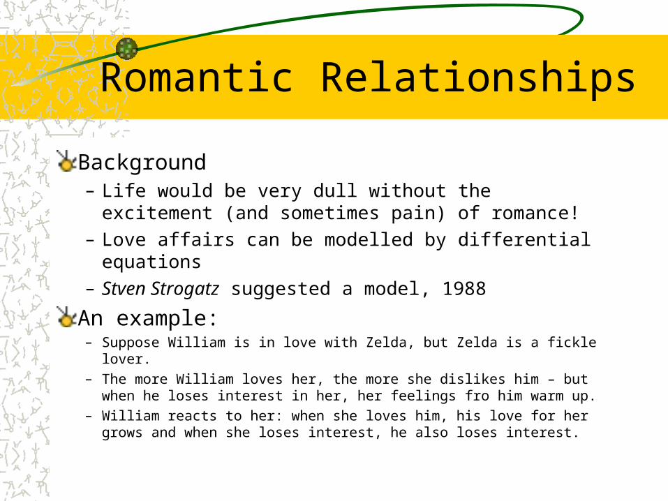
Romantic Relationships

Background– Life would be very dull without the excitement (and

sometimes pain) of romance! – Love affairs can be modelled by differential equations– Stven Strogatz suggested a model, 1988

An example: – Suppose William is in love with Zelda, but Zelda is a fickle lover. – The more William loves her, the more she dislikes him – but when he loses

interest in her, her feelings fro him warm up.– William reacts to her: when she loves him, his love for her grows and when she

loses interest, he also loses interest.

Romantic Relationships

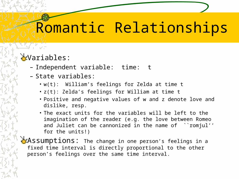
Variables:– Independent variable: time: t– State variables:

• w(t): William’s feelings for Zelda at time t• z(t): Zelda’s feelings for William at time t• Positive and negative values of w and z denote love and dislike, resp.• The exact units for the variables will be left to the imagination of the

reader (e.g. the love between Romeo and Juliet can be cannonized in the name of ``romjul’’ for the units!)

Assumptions: The change in one person’s feelings in a fixed time interval is directly proportional to the other person’s feelings over the same time interval.

Romantic Relationships

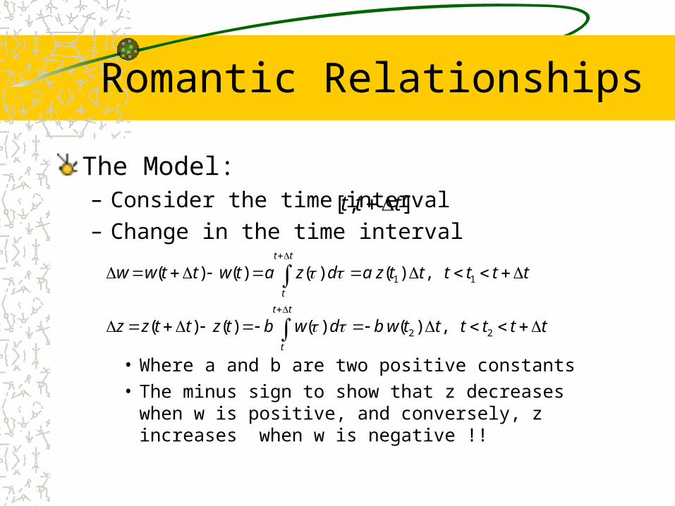
The Model: – Consider the time interval – Change in the time interval

• Where a and b are two positive constants• The minus sign to show that z decreases when w is positive, and

conversely, z increases when w is negative !!

[ , ]t t t

1 1

2 2

( ) ( ) ( ) ( ) ,

( ) ( ) ( ) ( ) ,

t t

t

t t

t

w w t t w t a z d a z t t t t t t

z z t t z t b w d b w t t t t t t

Romantic Relationships

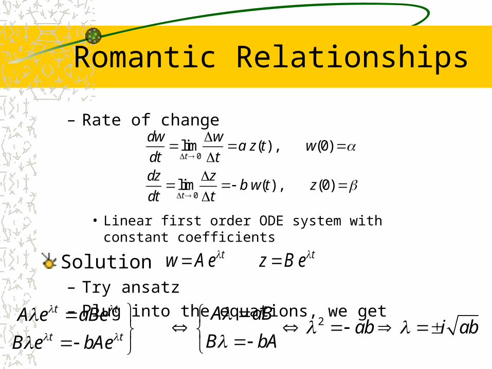
– Rate of change

• Linear first order ODE system with constant coefficients

Solution– Try ansatz– Plug into the equations, we get

0

0

lim ( ) , (0)

lim ( ) , (0)

t

t

dw wa z t w

dt tdz z

b w t zdt t

t tw A e z B e

2t t

t t

A aBA e aBeab i ab

B bAB e bAe

Romantic Relationships

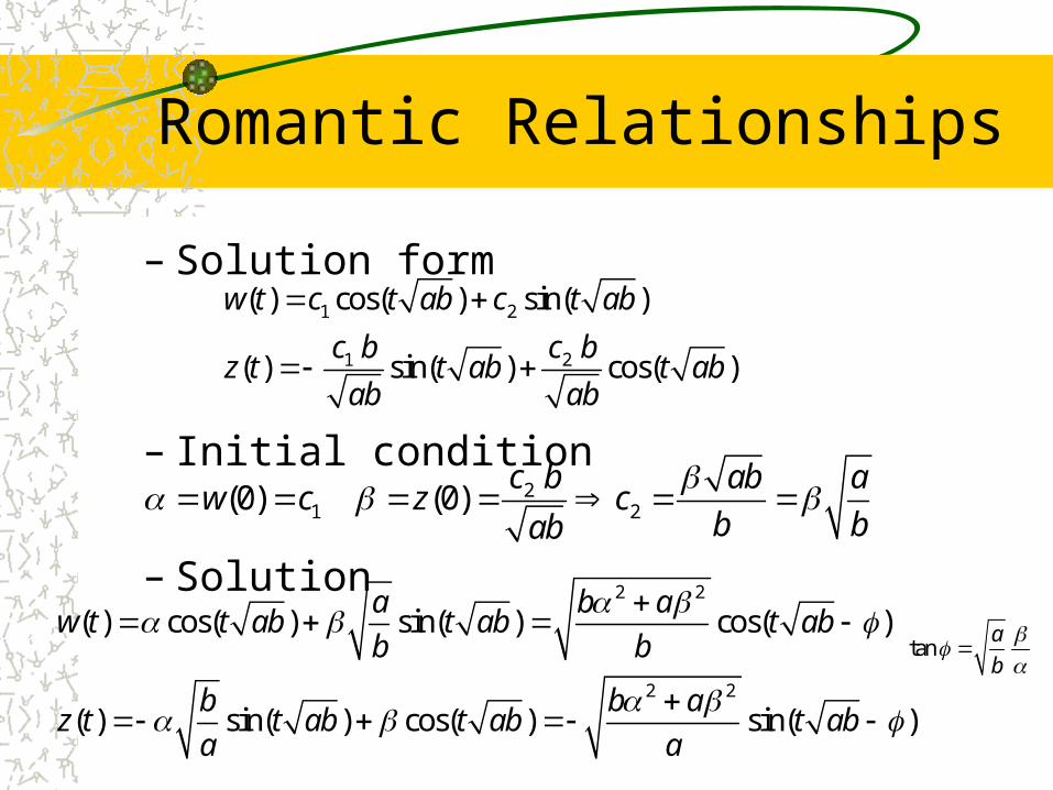
– Solution form

– Initial condition

– Solution

1 2

1 2

( ) cos( ) sin( )

( ) sin( ) cos( )

w t c t ab c t ab

c b c bz t t ab t ab

ab ab

21 2(0) (0)

c b ab aw c z c

b bab

2 2

2 2

( ) cos( ) sin( ) cos( )

( ) sin( ) cos( ) sin( )

a b aw t t ab t ab t ab

b b

b b az t t ab t ab t ab

a a

tana

b

Romantic Relationships

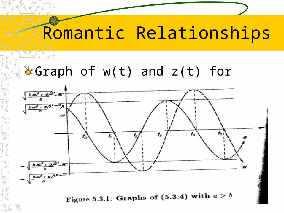
Graph of w(t) and z(t) for the case when a>b

Romantic Relationships

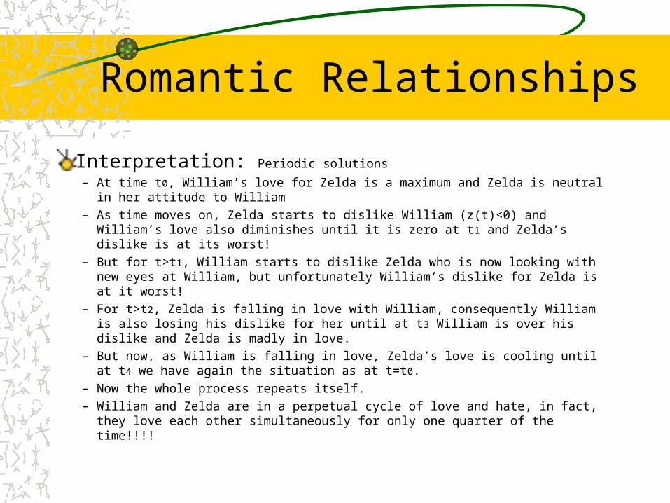
Interpretation: Periodic solutions– At time t0, William’s love for Zelda is a maximum and Zelda is neutral in her attitude to

William– As time moves on, Zelda starts to dislike William (z(t)<0) and William’s love also

diminishes until it is zero at t1 and Zelda’s dislike is at its worst!– But for t>t1, William starts to dislike Zelda who is now looking with new eyes at William,

but unfortunately William’s dislike for Zelda is at it worst!– For t>t2, Zelda is falling in love with William, consequently William is also losing his

dislike for her until at t3 William is over his dislike and Zelda is madly in love. – But now, as William is falling in love, Zelda’s love is cooling until at t4 we have again the

situation as at t=t0. – Now the whole process repeats itself.– William and Zelda are in a perpetual cycle of love and hate, in fact, they love each other

simultaneously for only one quarter of the time!!!!

Romantic Relationships

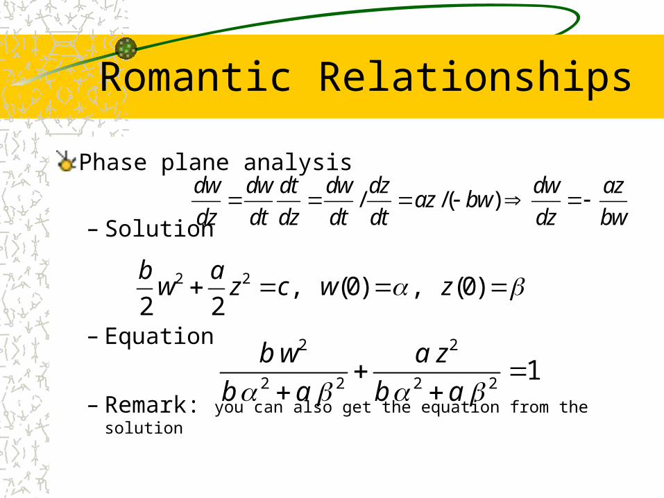
Phase plane analysis

– Solution

– Equation

– Remark: you can also get the equation from the solution

/ /( )dw dw dt dw dz dw az

az bwdz dt dz dt dt dz bw

2 2 , (0) , (0)2 2

b aw z c w z

2 2

2 2 2 21

b w a z

b a b a

Romantic Relationships

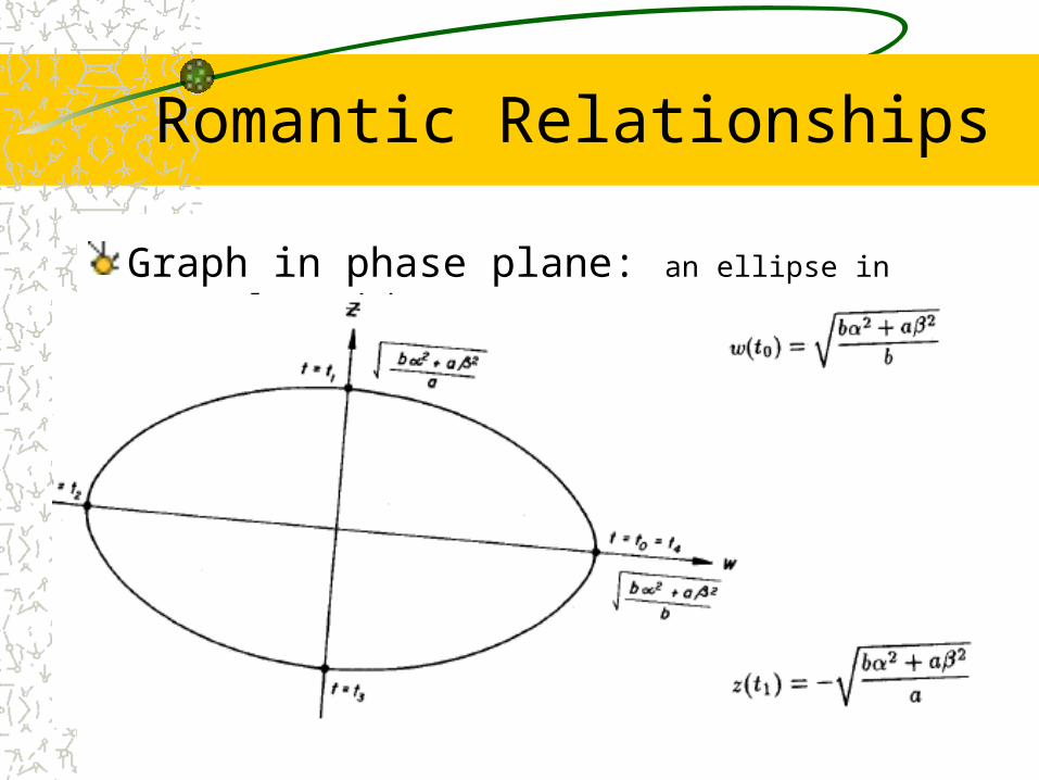
Graph in phase plane: an ellipse in (z,w)-plane with t as a parameter

Romantic Relationships

Interpretation: Periodic solutions– At time t0, William’s love for Zelda is a maximum and Zelda is neutral in her attitude to

William– As time moves on, Zelda starts to dislike William (z(t)<0) and William’s love also

diminishes until it is zero at t1 and Zelda’s dislike is at its worst!– But for t>t1, William starts to dislike Zelda who is now looking with new eyes at William,

but unfortunately William’s dislike for Zelda is at it worst!– For t>t2, Zelda is falling in love with William, consequently William is also losing his

dislike for her until at t3 William is over his dislike and Zelda is madly in love. – But now, as William is falling in love, Zelda’s love is cooling until at t4 we have again the

situation as at t=t0. – Now the whole process repeats itself.– William and Zelda are in a perpetual cycle of love and hate, in fact, they love each other

simultaneously for only one quarter of the time!!!!

Romantic Relationships

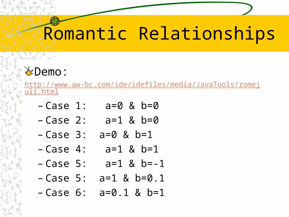
Demo: http://www.aw-bc.com/ide/idefiles/media/JavaTools/romejuli.html

– Case 1: a=0 & b=0– Case 2: a=1 & b=0– Case 3: a=0 & b=1– Case 4: a=1 & b=1– Case 5: a=1 & b=-1– Case 5: a=1 & b=0.1– Case 6: a=0.1 & b=1

Romantic Relationships

Two ways to look at the solutions w(t) & z(t)– First way: look at the graphs of w(t) & z(t) as

functions of t– Second way: eliminate the independent variable (if

possible) to obtain a relation between w and z.

Phase Plane: The plane whose points can be identified with coordinates on the (z,w)-axes. For autonomous system, we can always draw the phase plane.

Marriage

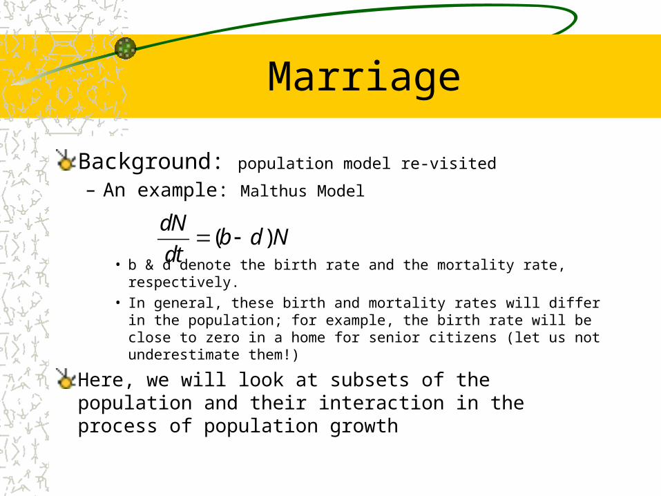
Background: population model re-visited

– An example: Malthus Model

• b & d denote the birth rate and the mortality rate, respectively.• In general, these birth and mortality rates will differ in the population; for

example, the birth rate will be close to zero in a home for senior citizens (let us not underestimate them!)

Here, we will look at subsets of the population and their interaction in the process of population growth

( )dN

b d Ndt

Marriage

We subdivide the population into three classes:– (i) unmarried males– (ii) unmarried females– (iii) married persons

Assumptions– The marriage is monogamous (a wife & a husband!!!)– A person who are married, but is now single due to divorce or

the death of the husband/wife, is unmarried– Only married couples produce children

Marriage

Interaction between different classes– Married couples produce children who are unmarried– Unmarried persons decide to get married – The growth of each of the three classes is interrelated!!

Variables– Independent variable: time: t– State variables:

• m(t): number of unmarried males in the population at time t• f(t): number of unmarried females in the population at time t• w(t): number of married couples in the population at time t

Marriage

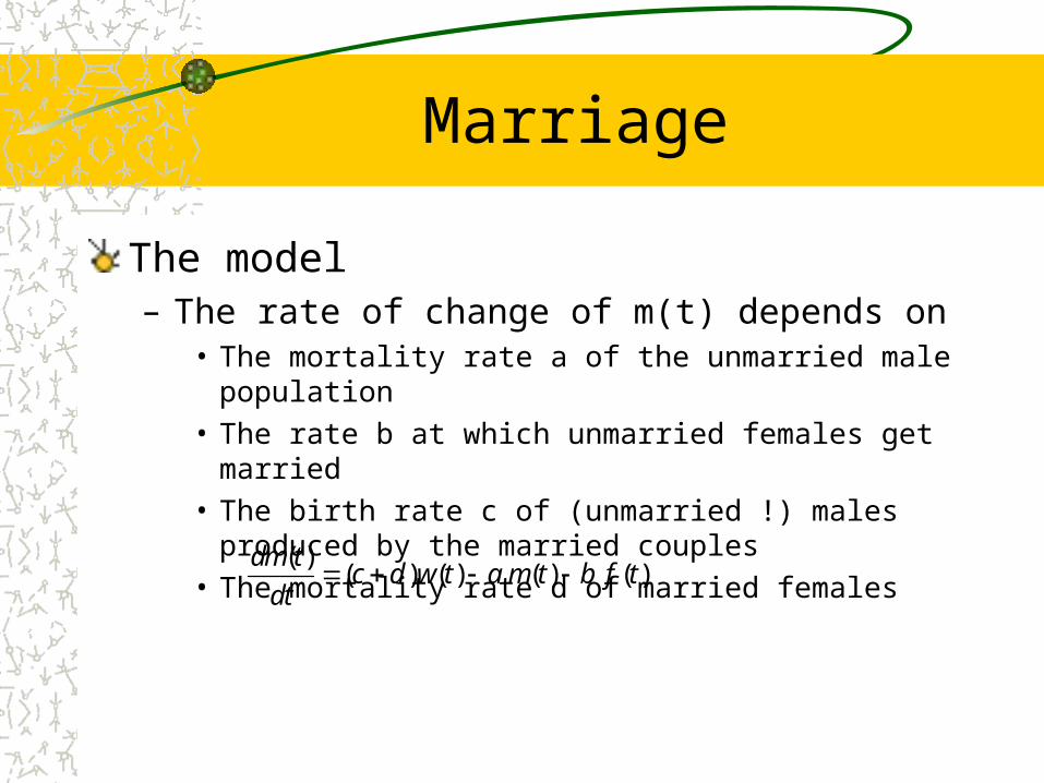
The model– The rate of change of m(t) depends on

• The mortality rate a of the unmarried male population• The rate b at which unmarried females get married• The birth rate c of (unmarried !) males produced by the married

couples• The mortality rate d of married females

( )( ) ( ) ( ) ( )

dm tc d w t a m t b f t

dt

Marriage

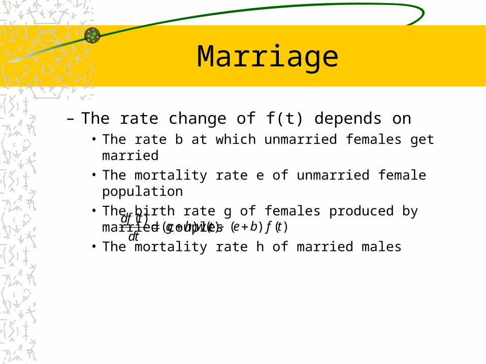
– The rate change of f(t) depends on• The rate b at which unmarried females get married• The mortality rate e of unmarried female population• The birth rate g of females produced by married couples• The mortality rate h of married males

( )( ) ( ) ( ) ( )

df tg h w t e b f t

dt

Marriage

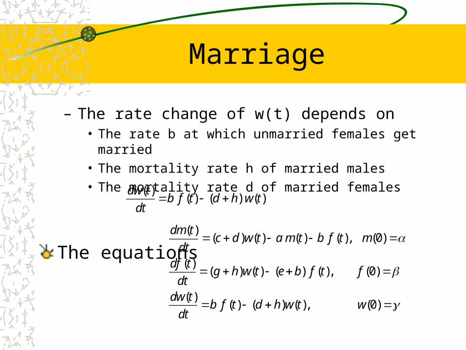
– The rate change of w(t) depends on• The rate b at which unmarried females get married• The mortality rate h of married males• The mortality rate d of married females

The equations

( )( ) ( ) ( )

dw tb f t d h w t

dt

( )( ) ( ) ( ) ( ), (0)

( )( ) ( ) ( ) ( ), (0)

( )( ) ( ) ( ), (0)

dm tc d w t a m t b f t m

dtdf t

g h w t e b f t fdtdw t

b f t d h w t wdt

Marriage

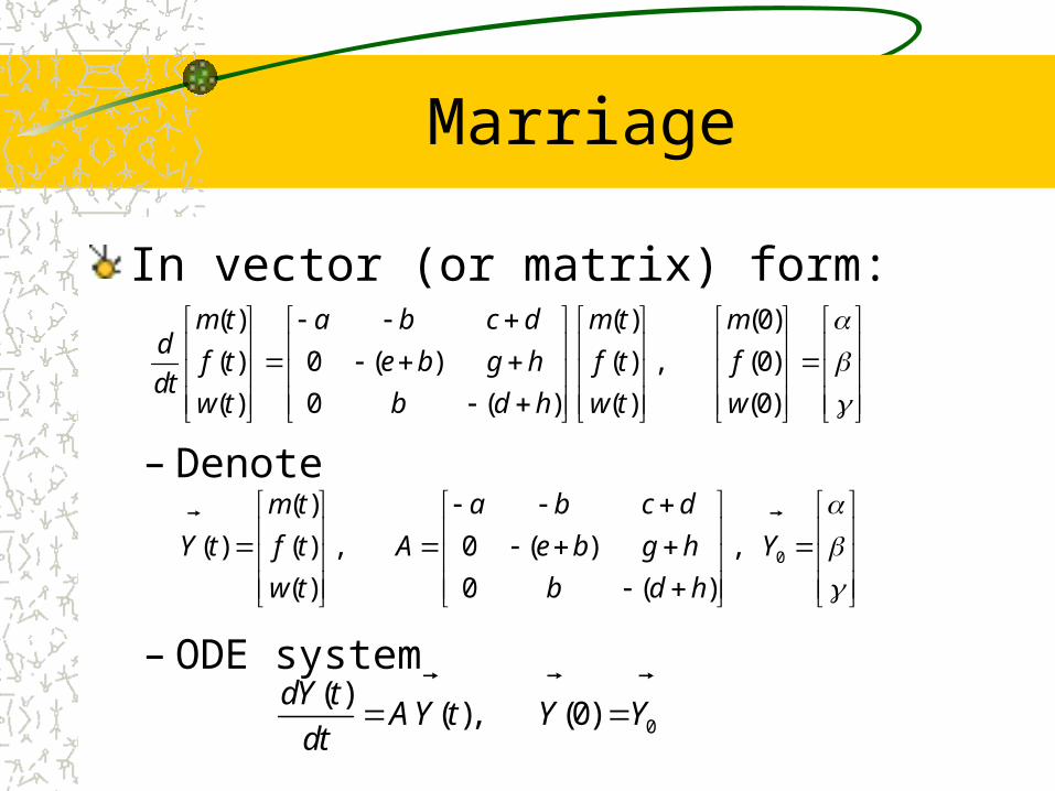
In vector (or matrix) form:

– Denote

– ODE system

0

( )

( ) ( ) , 0 ( ) ,

( ) 0 ( )

m t a b c d

Y t f t A e b g h Y

w t b d h

( ) ( ) (0)

( ) 0 ( ) ( ) , (0)

( ) 0 ( ) ( ) (0)

m t a b c d m t md

f t e b g h f t fdtw t b d h w t w

0

( )( ), (0)

dY tAY t Y Y

dt

Marriage

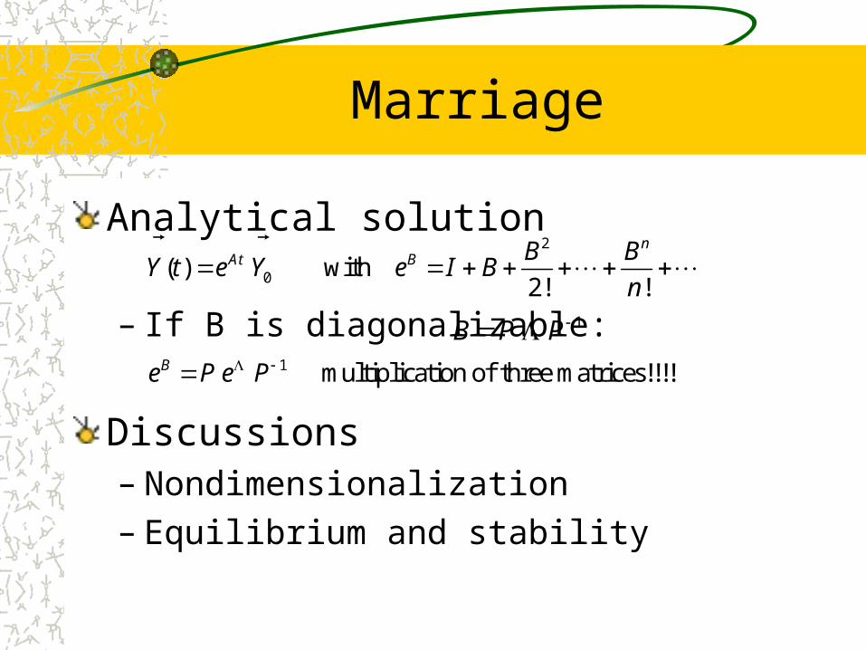
Analytical solution

– If B is diagonalizable:

Discussions – Nondimensionalization– Equilibrium and stability

2

0( ) with2! !

nAt B B B

Y t e Y e I Bn

1B P P 1 multiplication of three matrices!!!!Be P e P

Analytic & Numerical Solutions of 1st Order ODEs

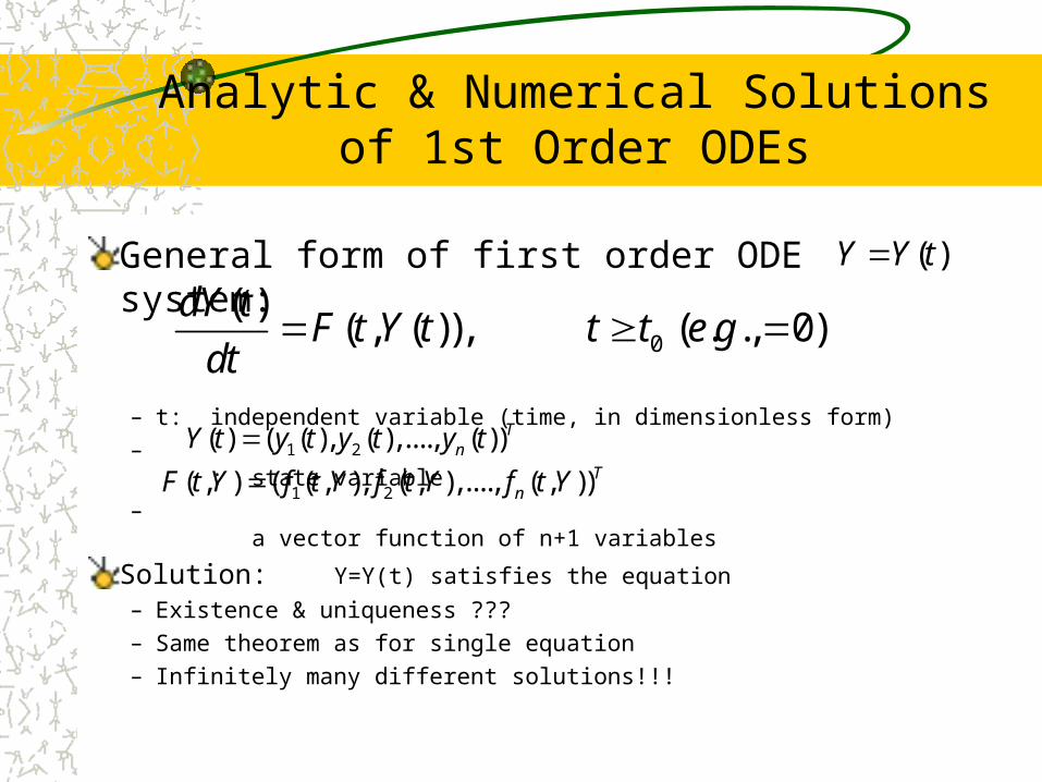
General form of first order ODE system:

– t: independent variable (time, in dimensionless form) – : state variable – a vector function of n+1 variables

Solution: Y=Y(t) satisfies the equation– Existence & uniqueness ???– Same theorem as for single equation– Infinitely many different solutions!!!

( )Y Y t

0

( )( , ( )), ( . ., 0)

dY tF t Y t t t e g

dt

1 2( ) ( ( ), ( ),...., ( ))TnY t y t y t y t

1 2( , ) ( ( , ), ( , ),...., ( , ))TnF t Y f t Y f t Y f t Y

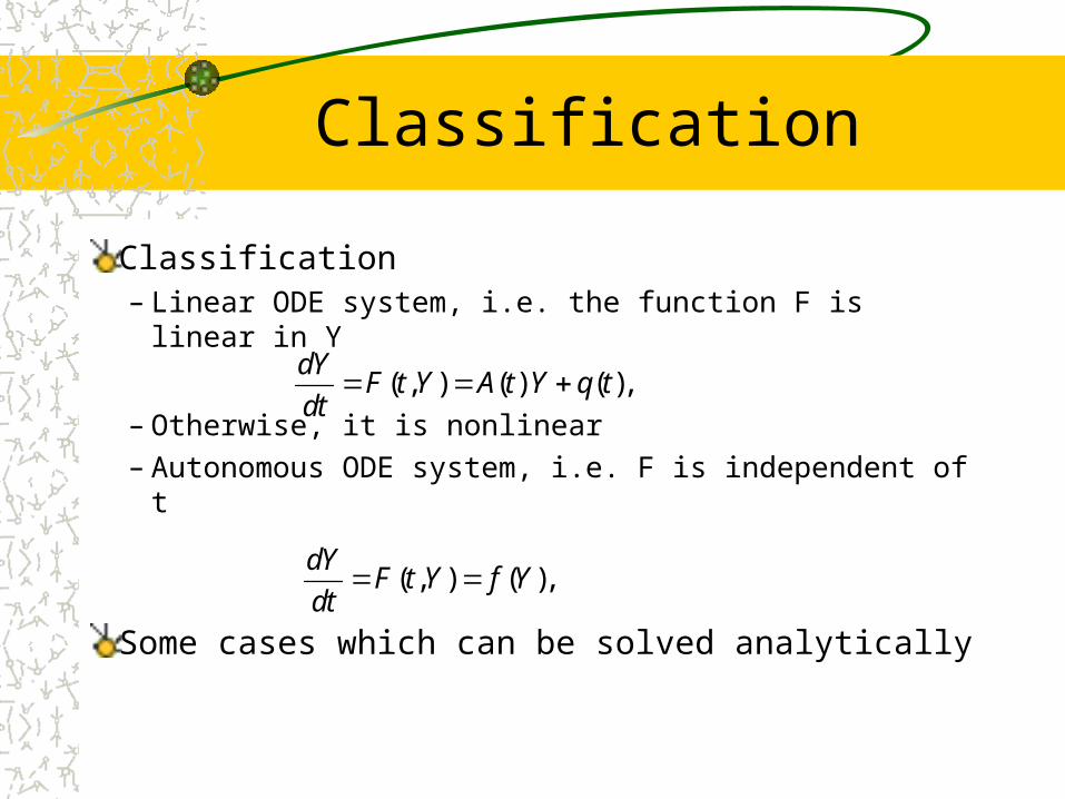
Classification

Classification– Linear ODE system, i.e. the function F is linear in Y

– Otherwise, it is nonlinear – Autonomous ODE system, i.e. F is independent of t

Some cases which can be solved analytically

( , ) ( ),dY

F t Y f Ydt

( , ) ( ) ( ),dY

F t Y A t Y q tdt

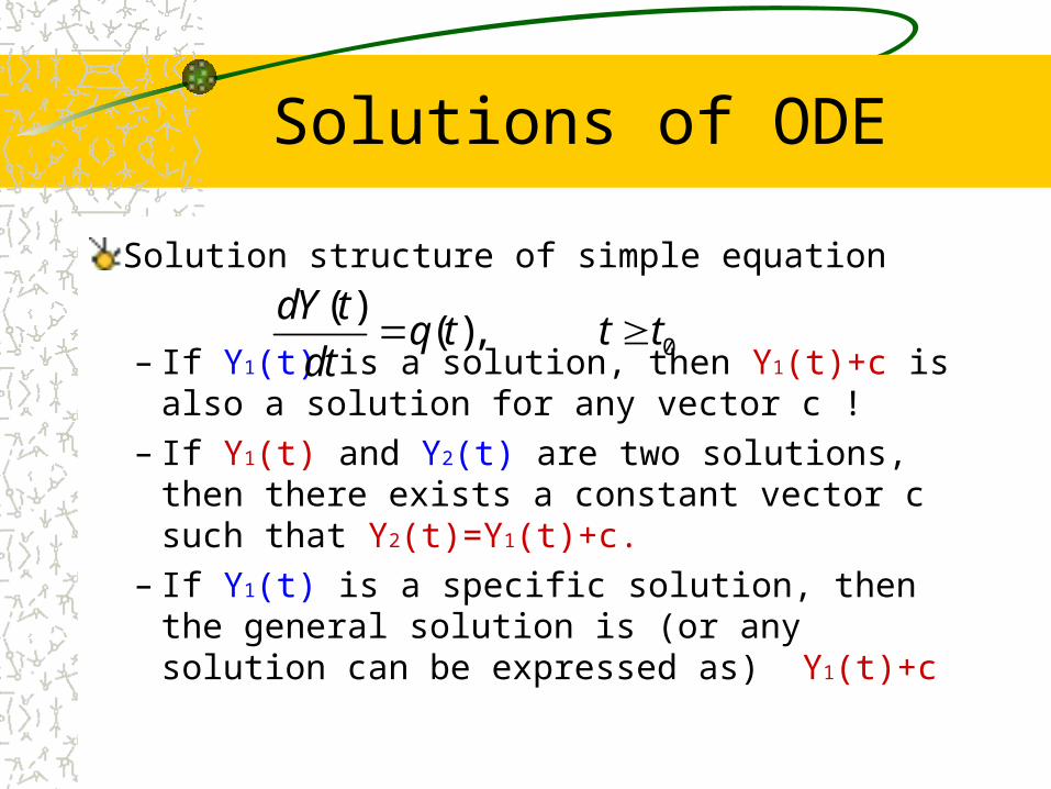
Solutions of ODE

Solution structure of simple equation

– If Y1(t) is a solution, then Y1(t)+c is also a solution for any vector c !

– If Y1(t) and Y2(t) are two solutions, then there exists a constant vector c such that Y2(t)=Y1(t)+c.

– If Y1(t) is a specific solution, then the general solution is (or any solution can be expressed as) Y1(t)+c

0

( )( ),

dY tq t t t

dt

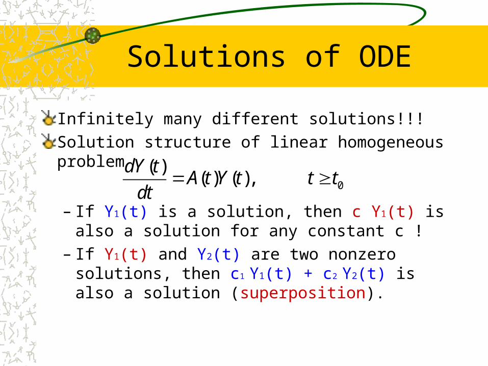
Solutions of ODE

Infinitely many different solutions!!!Solution structure of linear homogeneous problem

– If Y1(t) is a solution, then c Y1(t) is also a solution for any constant c !

– If Y1(t) and Y2(t) are two nonzero solutions, then c1

Y1(t) + c2 Y2(t) is also a solution (superposition).

0

( )( ) ( ),

dY tA t Y t t t

dt

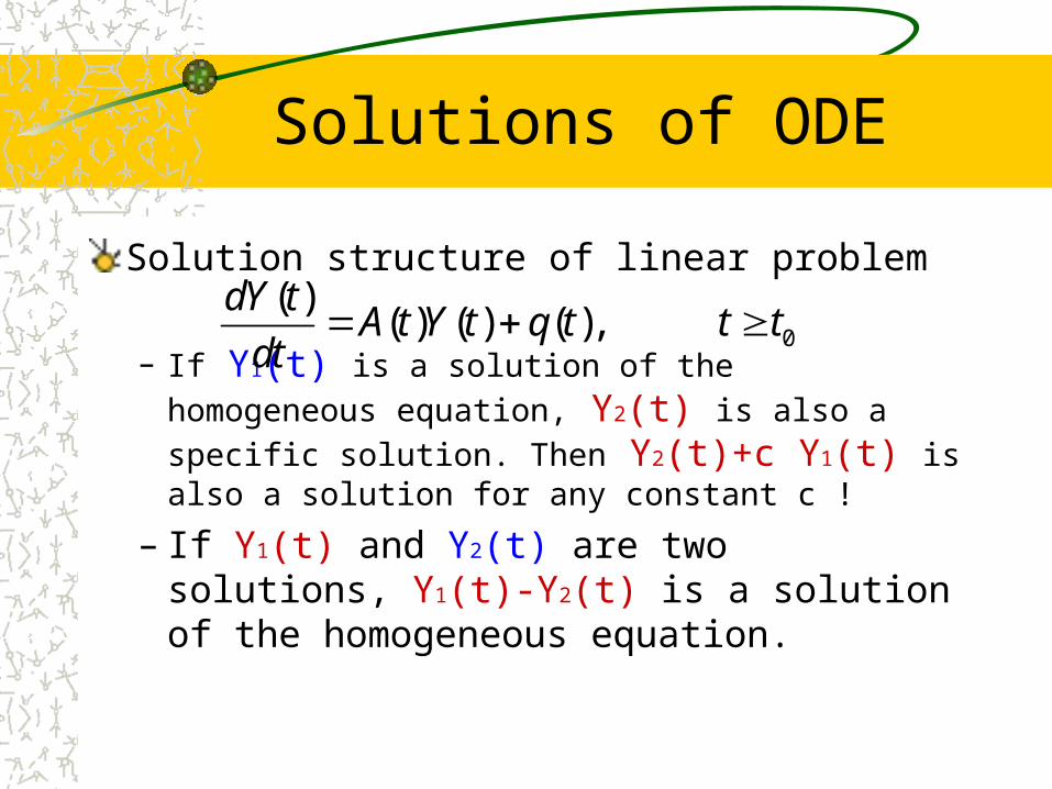
Solutions of ODE

Solution structure of linear problem

– If Y1(t) is a solution of the homogeneous equation, Y2(t) is also a specific solution. Then Y2(t)+c Y1(t) is also a solution for any constant c !

– If Y1(t) and Y2(t) are two solutions, Y1(t)-Y2(t) is a solution of the homogeneous equation.

0

( )( ) ( ) ( ),

dY tA t Y t q t t t

dt

Solutions of IVP

Initial value problem (IVP):

Solution: – Existence – Uniqueness

0 0 0

( )( , ( )), ; ( )

dY tF t Y t t t Y t Y

dt

Solutions of IVP

Theorem: Suppose that the real-valued function F(t,Y) is continuous on some rectangle in the (t,Y)-plane containing the point (t0,Y0) in its interior. Then the above initial value problem has at least one solution defined on some open interval J containing the point t0. If, in addition, the partial derivative is continuous on that rectangle, then the solution is unique on some (perhaps smaller) open interval J0 containing the point t=t0.

Proof: Omitted

/F y

Solution: Case I

– F is independent of y, i.e.

• Analytical solution

• Example 1:

– Solution

1 1

22 2

( ) (0)1 sin 1,

( ) (0)cos 3 0

y t yt td

y t yt tdt

2

1

0

2 32

0

( ) 1 (1 sin ) 2 cos2

( ) 0 (cos 3 ) sin

t

t

ty t s s ds t t

y t s s ds t t

0

0

( ) ( )t

Y t Y q s ds

0( ), (0)d Y

q t Y Yd t

( , ) ( )F t Y q t

Solution: case II

Linear homogeneous system

Analytical solution

– If B is diagonalizable:

– The solution– An example

0

( )( ), (0)

dY tAY t Y Y

dt

2

0( ) with2! !

nAt B B B

Y t e Y e I Bn

1 multiplication of three matrices!!!!Be P e P

10( ) tY t P e P Y

Equilibrium & stability

Consider autonomous ODE

Equilibrium:Asymptotically stable: Conditions:– Stable:real parts of all eigenvalues of the Jacobian matrix are negative

– Unstable: at least the real part of one eigenvalue of the Jacobian matrix is positive

( )( )

dY tF Y

dt

* satisfying F( *) 0Y Y

( ) * 0 whenY t Y t

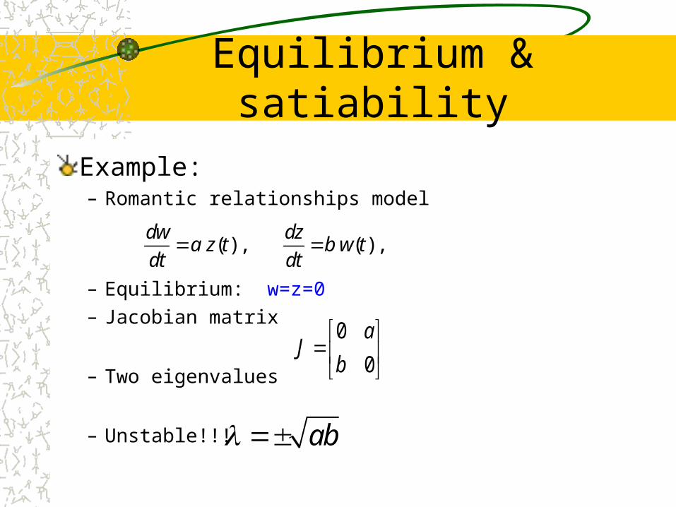
Equilibrium & satiability

Example: – Romantic relationships model

– Equilibrium: w=z=0– Jacobian matrix

– Two eigenvalues

– Unstable!!!

( ) , ( ) ,dw dz

a z t b w tdt dt

0

0

aJ

b

ab

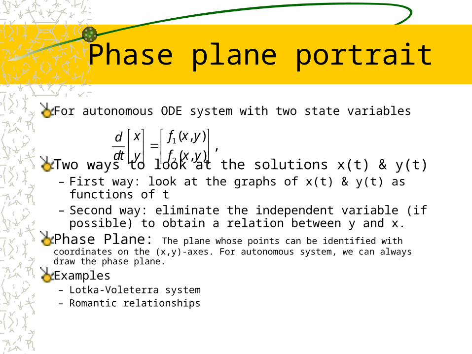
Phase plane portrait

For autonomous ODE system with two state variables

Two ways to look at the solutions x(t) & y(t)– First way: look at the graphs of x(t) & y(t) as functions of t– Second way: eliminate the independent variable (if possible) to

obtain a relation between y and x. Phase Plane: The plane whose points can be identified with coordinates on the (x,y)-axes. For autonomous system, we can always draw the phase plane.

Examples– Lotka-Voleterra system– Romantic relationships

1

2

( , ),

( , )

f x yxd

f x yydt

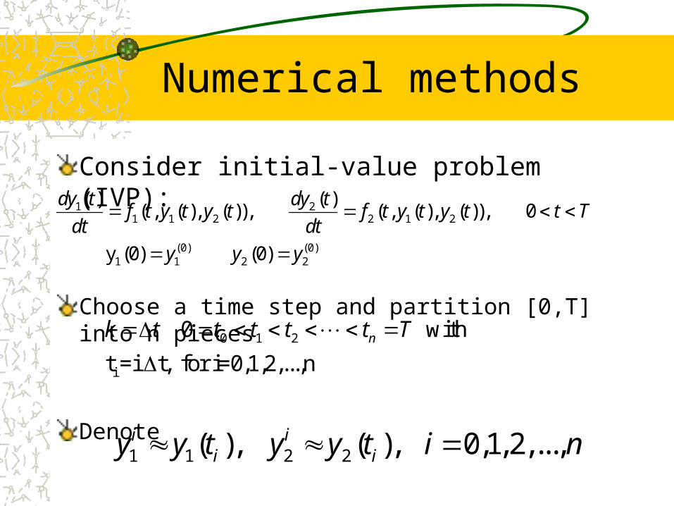
Numerical methods

Consider initial-value problem (IVP):

Choose a time step and partition [0,T] into n pieces

Denote

1 21 1 2 2 1 2

(0) (0)1 1 2 2

( ) ( )( , ( ), ( )), ( , ( ), ( )), 0

y (0) (0)

dy t dy tf t y t y t f t y t y t t T

dt dt

y y y

0 1 2

i

0 with

t =i t, for i=0,1,2,...,n nk t t t t t T

1 1 2 2( ), ( ), 0,1,2,...,i ii iy y t y y t i n

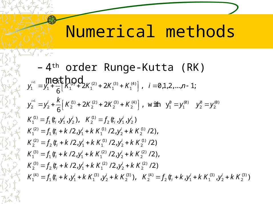
Numerical methods

– 4th order Runge-Kutta (RK) method1

1

(1) (2) (3) (4)1 1 1 1 1 1

(1) (2) (3) (4) 0 (0) 0 (0)2 2 2 2 2 2 1 1 2 2

(1) (1)1 1 1 2 2 2 1 2

(2) (1)1 1 1 1

2 2 , 0,1,2,..., 1; 6

2 2 , with y6

( , , ), ( , , )

( / 2, /

i

i

i

i

i i i ii i

ii

ky y K K K K i n

ky y K K K K y y y

K f t y y K f t y y

K f t k y k K

(1)2 2

(2) (1) (1)2 2 1 1 2 2

(3) (2) (2)1 1 1 1 2 2

(3) (2) (2)2 2 1 1 2 2

(4) (3) (3) (4)1 1 1 1 2 2 2 2 1

2, / 2),

( / 2, / 2, / 2)

( / 2, / 2, / 2),

( / 2, / 2, / 2)

( , , ), ( ,

i

i ii

i ii

i ii

i i ii i

y k K

K f t k y k K y k K

K f t k y k K y k K

K f t k y k K y k K

K f t k y k K y k K K f t k y k K

(3) (3)1 2 2, )iy k K