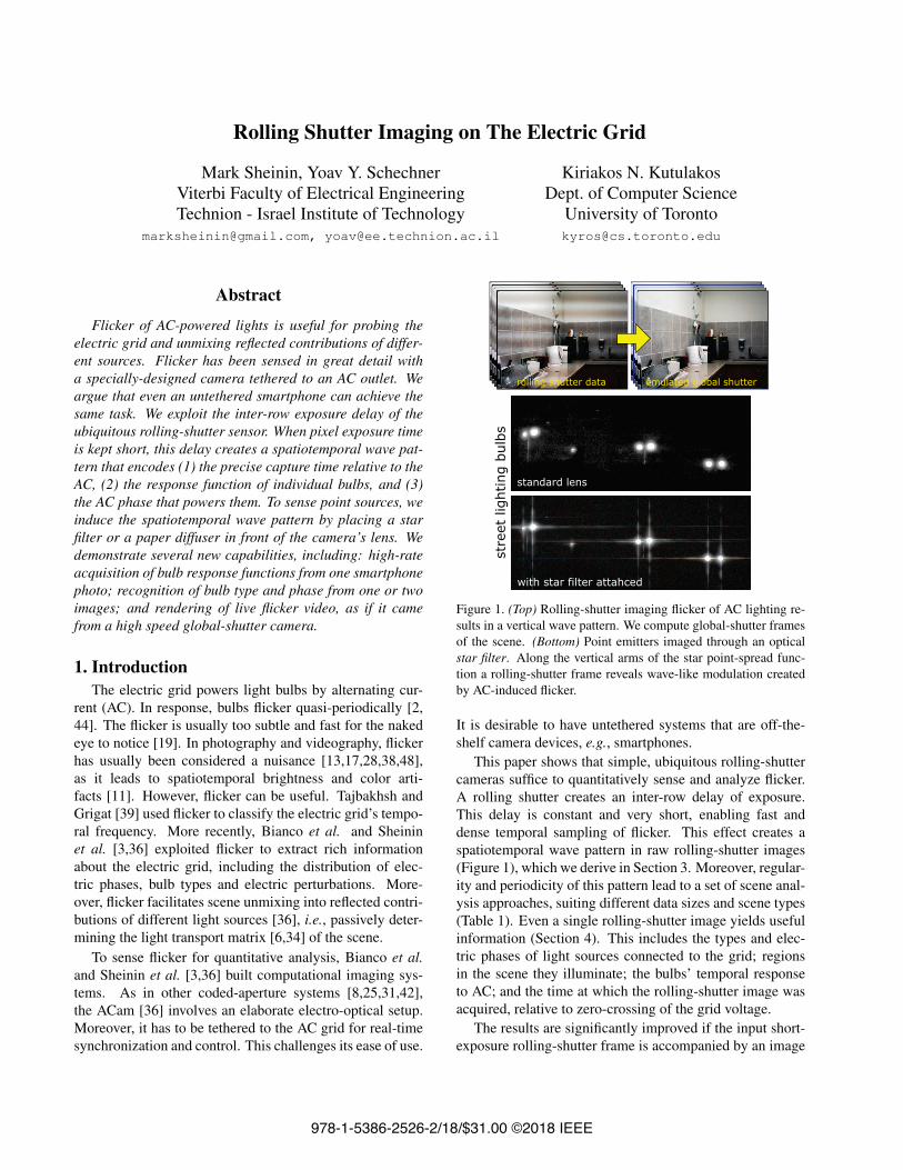
Rolling Shutter Imaging on The Electric Grid

Mark Sheinin, Yoav Y. SchechnerViterbi Faculty of Electrical EngineeringTechnion - Israel Institute of Technology

marksheinin@gmail.com, yoav@ee.technion.ac.il

Kiriakos N. KutulakosDept. of Computer Science

University of Torontokyros@cs.toronto.edu

Abstract

Flicker of AC-powered lights is useful for probing theelectric grid and unmixing reflected contributions of differ-ent sources. Flicker has been sensed in great detail witha specially-designed camera tethered to an AC outlet. Weargue that even an untethered smartphone can achieve thesame task. We exploit the inter-row exposure delay of theubiquitous rolling-shutter sensor. When pixel exposure timeis kept short, this delay creates a spatiotemporal wave pat-tern that encodes (1) the precise capture time relative to theAC, (2) the response function of individual bulbs, and (3)the AC phase that powers them. To sense point sources, weinduce the spatiotemporal wave pattern by placing a starfilter or a paper diffuser in front of the camera’s lens. Wedemonstrate several new capabilities, including: high-rateacquisition of bulb response functions from one smartphonephoto; recognition of bulb type and phase from one or twoimages; and rendering of live flicker video, as if it camefrom a high speed global-shutter camera.

1. IntroductionThe electric grid powers light bulbs by alternating cur-

rent (AC). In response, bulbs flicker quasi-periodically [2,

44]. The flicker is usually too subtle and fast for the naked

eye to notice [19]. In photography and videography, flicker

has usually been considered a nuisance [13,17,28,38,48],

as it leads to spatiotemporal brightness and color arti-

facts [11]. However, flicker can be useful. Tajbakhsh and

Grigat [39] used flicker to classify the electric grid’s tempo-

ral frequency. More recently, Bianco et al. and Sheinin

et al. [3,36] exploited flicker to extract rich information

about the electric grid, including the distribution of elec-

tric phases, bulb types and electric perturbations. More-

over, flicker facilitates scene unmixing into reflected contri-

butions of different light sources [36], i.e., passively deter-

mining the light transport matrix [6,34] of the scene.

To sense flicker for quantitative analysis, Bianco et al.and Sheinin et al. [3,36] built computational imaging sys-

tems. As in other coded-aperture systems [8,25,31,42],

the ACam [36] involves an elaborate electro-optical setup.

Moreover, it has to be tethered to the AC grid for real-time

synchronization and control. This challenges its ease of use.

Figure 1. (Top) Rolling-shutter imaging flicker of AC lighting re-

sults in a vertical wave pattern. We compute global-shutter frames

of the scene. (Bottom) Point emitters imaged through an optical

star filter. Along the vertical arms of the star point-spread func-

tion a rolling-shutter frame reveals wave-like modulation created

by AC-induced flicker.

It is desirable to have untethered systems that are off-the-

shelf camera devices, e.g., smartphones.

This paper shows that simple, ubiquitous rolling-shutter

cameras suffice to quantitatively sense and analyze flicker.

A rolling shutter creates an inter-row delay of exposure.

This delay is constant and very short, enabling fast and

dense temporal sampling of flicker. This effect creates a

spatiotemporal wave pattern in raw rolling-shutter images

(Figure 1), which we derive in Section 3. Moreover, regular-

ity and periodicity of this pattern lead to a set of scene anal-

ysis approaches, suiting different data sizes and scene types

(Table 1). Even a single rolling-shutter image yields useful

information (Section 4). This includes the types and elec-

tric phases of light sources connected to the grid; regions

in the scene they illuminate; the bulbs’ temporal response

to AC; and the time at which the rolling-shutter image was

acquired, relative to zero-crossing of the grid voltage.

The results are significantly improved if the input short-

exposure rolling-shutter frame is accompanied by an image

978-1-5386-2526-2/18/$31.00 ©2018 IEEE

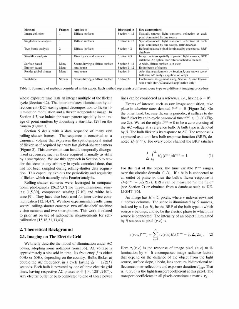
Method Frames Applies to Discussed in Key assumptionsImage deflicker 1 Diffuse surfaces Section 4.1.1 Spatially-smooth light transport, reflection at each

pixel dominated by one source

Single-frame analysis 1 Diffuse surfaces Section 4.1.2 Spatially-smooth light transport, reflection at each

pixel dominated by one source, BRF database

Two-frame analysis 2 Diffuse surfaces Section 4.2 Reflection at each pixel dominated by one source, BRF

database

Star-filter analysis 2 Directly viewed sources Section 4.3 Image contains spatially separated light sources, BRF

database, An optical star-filter attached to the lens

Surface-based Many Scenes having a diffuse surface Section 5.1.1 A wide, diffuse surface is in view

Emitter-based Many Any scene Section 5.1.2 Entire batch of frames

Render global shutter Many Any scene Section 6 After frame assignment by Section 5, one known scene

bulb (for AC analysis application only)

Real-time Stream Scenes having a diffuse surface Section 6 Continuous assignment using Section 5, one known

scene bulb (for AC analysis application only)

Table 1. Summary of methods considered in this paper. Each method represents a different scene type or a different imaging procedure.

whose exposure time lasts an integer multiple of the flicker

cycle (Section 4.2). The latter emulates illumination by di-

rect current (DC), easing signal decomposition to flicker il-

lumination modulation and a flicker independent image. In

Section 4.3, we induce the wave pattern spatially in an im-

age of point emitters by mounting a star-filter [29] on the

camera (Figure 1).

Section 5 deals with a data sequence of many raw

rolling-shutter frames. The sequence is converted to a

canonical volume that expresses the spatiotemporal signal

of flicker, as if acquired by a very fast global-shutter camera

(Figure 2). This conversion can handle temporally disorga-

nized sequences, such as those acquired manually as stills

by a smartphone. We use this approach in Section 6 to ren-

der the scene at any arbitrary in-cycle canonical time, that

had not been sampled during rolling-shutter data acquisi-

tion. This capability exploits the periodicity and regularity

of flicker, which naturally suits Fourier analysis.

Rolling-shutter cameras were leveraged in computa-

tional photography [26,27,37] for three-dimensional sens-

ing [1,5,30], compressed sensing [7,10] and white bal-

ance [9]. They have also been used for inter-device com-

munication [12,14,47]. We show experimental results using

several rolling-shutter cameras: two off-the-shelf machine

vision cameras and two smartphones. This work is related

to prior art on use of radiometric measurements for self-

calibration [15,18,31,33,43].

2. Theoretical Background2.1. Imaging on The Electric Grid

We briefly describe the model of illumination under AC

power, adopting some notations from [36]. AC voltage is

approximately a sinusoid in time. Its frequency f is either

50Hz or 60Hz, depending on the country. Bulbs flicker at

double the AC frequency, in a cycle lasting Δ = 1/(2f)seconds. Each bulb is powered by one of three electric grid

lines, having respective AC phases φ ∈ {0◦, 120◦, 240◦}.Any electric outlet or bulb connected to one of these power

lines can be considered as a reference, i.e., having φ = 0◦.Events of interest, such as raw image acquisition, take

place in absolute time, denoted tabs ∈ R (Figure 2a). On

the other hand, because flicker is periodic, it suffices to de-

fine flicker by an in-cycle canonical time tcan ∈ [0,Δ] (Fig-ure 2c). We set the origin tcan=0 to be a zero crossing of

the AC voltage at a reference bulb. A bulb type is denoted

by β. The bulb flicker is its response to AC. The response is

expressed as a unit-less bulb response function (BRF), de-

noted Bβ(tcan). For every color channel the BRF satisfies

1

Δ

∫ Δ

0

Bβ(tcan)dtcan = 1. (1)

For the rest of the paper, the time variable tcan ranges

over the circular domain [0,Δ]. If a bulb is connected to

an outlet of phase φ, then the bulb’s flicker response is

Bβ(tcan − φΔ/2π). BRFs can be measured “in the field”

(see Section 7) or obtained from a database such as DE-

LIGHT [36].

An image has R × C pixels, where r indexes rows and

c indexes columns. The scene is illuminated by S sources,

indexed by s. Let Bs be the BRF of the bulb type to which

source s belongs, and φs be the electric phase to which this

source is connected. The intensity of an object illuminated

by S sources at pixel (r, c) is

i(r, c, tcan) =S∑

s=1

τs(r, c)Bs(tcan − φsΔ/2π). (2)

Here τs(r, c) is the response of image pixel (r, c) to il-

lumination by s. It encompasses image radiance factors

that depend on the distance of the object from the light

source, surface slope, albedo, lens aperture, bidirectional re-

flectance, inter-reflections and exposure duration Texp. That

is, τs(r, c) is the light transport coefficient at this pixel. The

transport coefficients in all pixels constitute a matrix τs.

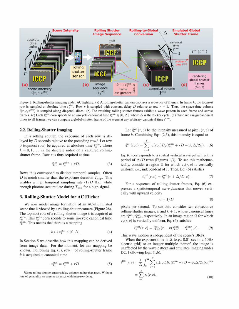
Figure 2. Rolling-shutter imaging under AC lighting. (a) A rolling-shutter camera captures a sequence of frames. In frame k, the topmost

row is sampled at absolute time tabsk . Row r is sampled with constant delay D relative to row r − 1. Thus, the space-time volume

i(r, c, tabs) is sampled along diagonal slices. (b) The resulting rolling-shutter frames exhibit a wave pattern in each frame and across

frames. (c) Each tabsk corresponds to an in-cycle canonical time tcank ∈ [0,Δ], where Δ is the flicker cycle. (d) Once we assign canonical

times to all frames, we can compute a global-shutter frame of the scene at any arbitrary canonical time tcan.

2.2. Rolling-Shutter ImagingIn a rolling shutter, the exposure of each row is de-

layed by D seconds relative to the preceding row.1 Let row

0 (topmost row) be acquired at absolute time tabsk , where

k = 0, 1, . . . is the discrete index of a captured rolling-

shutter frame. Row r is thus acquired at time

tabsk,r = tabsk + rD. (3)

Rows thus correspond to distinct temporal samples. Often

D is much smaller than the exposure duration Texp. This

enables a high temporal sampling rate (1/D Hz), while

enough photons accumulate during Texp for a high signal.

3. Rolling-Shutter Model for AC FlickerWe now model image formation of an AC-illuminated

scene that is viewed by a rolling-shutter camera (Figure 2b).

The topmost row of a rolling-shutter image k is acquired at

tabsk . This tabsk corresponds to some in-cycle canonical time

tcank . This means that there is a mapping

k �→ tcank ∈ [0,Δ]. (4)

In Section 5 we describe how this mapping can be derived

from image data. For the moment, let this mapping be

known. Following Eq. (3), row r of rolling-shutter frame

k is acquired at canonical time

tcank,r = tcank + rD. (5)

1Some rolling-shutter sensors delay columns rather than rows. Without

loss of generality we assume a sensor with inter-row delay.

Let irollk (r, c) be the intensity measured at pixel (r, c) offrame k. Combining Eqs. (2,5), this intensity is equal to

irollk (r, c) =

S∑s=1

τs(r, c)Bs(tcank + rD − φsΔ/2π). (6)

Eq. (6) corresponds to a spatial vertical wave pattern with a

period of Δ/D rows (Figures 1,3). To see this mathemat-

ically, consider a region Ω for which τs(r, c) is vertically

uniform, i.e., independent of r. Then, Eq. (6) satisfies

irollk (r, c) = irollk (r +Δ/D, c) . (7)

For a sequence of rolling-shutter frames, Eq. (6) ex-

presses a spatiotemporal wave function that moves verti-

cally with upward velocity

v = 1/D (8)

pixels per second. To see this, consider two consecutive

rolling-shutter images, k and k + 1, whose canonical times

are tcank , tcank+1, respectively. In an image region Ω for which

τs(r, c) is vertically uniform, Eq. (6) satisfies

irollk (r, c) = irollk+1(r − v(tcank+1 − tcank

), c) . (9)

This wave motion is independent of the scene’s BRFs.When the exposure time is Δ (e.g., 0.01 sec in a 50Hz

electric grid) or an integer multiple thereof, the image isunaffected by the wave pattern and emulates imaging underDC. Following Eqs. (1,6),

iDC(r, c) =1

Δ

∫ Δ

0

S∑s=1

τs(r, c)Bs(tcank + rD − φsΔ/2π)dt

can

=

S∑s=1

τs(r, c).(10)

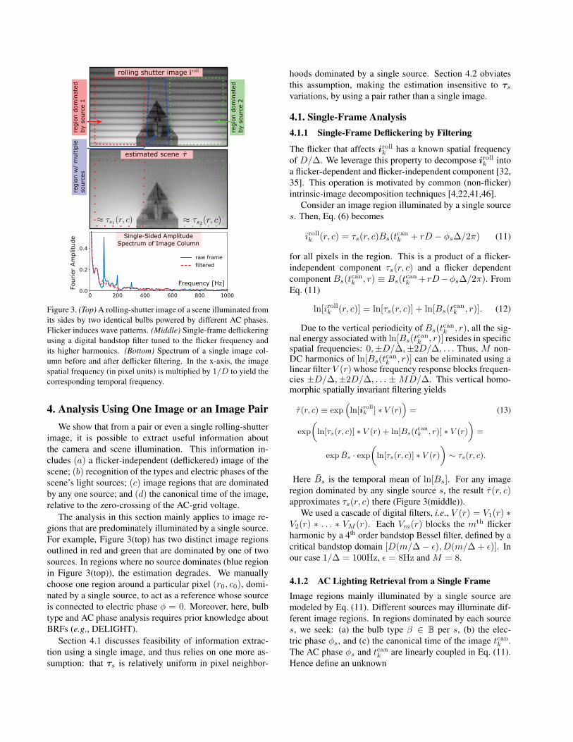
Figure 3. (Top) A rolling-shutter image of a scene illuminated from

its sides by two identical bulbs powered by different AC phases.

Flicker induces wave patterns. (Middle) Single-frame deflickering

using a digital bandstop filter tuned to the flicker frequency and

its higher harmonics. (Bottom) Spectrum of a single image col-

umn before and after deflicker filtering. In the x-axis, the image

spatial frequency (in pixel units) is multiplied by 1/D to yield the

corresponding temporal frequency.

4. Analysis Using One Image or an Image PairWe show that from a pair or even a single rolling-shutter

image, it is possible to extract useful information about

the camera and scene illumination. This information in-

cludes (a) a flicker-independent (deflickered) image of the

scene; (b) recognition of the types and electric phases of the

scene’s light sources; (c) image regions that are dominated

by any one source; and (d) the canonical time of the image,

relative to the zero-crossing of the AC-grid voltage.

The analysis in this section mainly applies to image re-

gions that are predominately illuminated by a single source.

For example, Figure 3(top) has two distinct image regions

outlined in red and green that are dominated by one of two

sources. In regions where no source dominates (blue region

in Figure 3(top)), the estimation degrades. We manually

choose one region around a particular pixel (r0, c0), domi-

nated by a single source, to act as a reference whose source

is connected to electric phase φ = 0. Moreover, here, bulb

type and AC phase analysis requires prior knowledge about

BRFs (e.g., DELIGHT).

Section 4.1 discusses feasibility of information extrac-

tion using a single image, and thus relies on one more as-

sumption: that τs is relatively uniform in pixel neighbor-

hoods dominated by a single source. Section 4.2 obviates

this assumption, making the estimation insensitive to τsvariations, by using a pair rather than a single image.

4.1. Single-Frame Analysis4.1.1 Single-Frame Deflickering by Filtering

The flicker that affects irollk has a known spatial frequency

of D/Δ. We leverage this property to decompose irollk into

a flicker-dependent and flicker-independent component [32,

35]. This operation is motivated by common (non-flicker)

intrinsic-image decomposition techniques [4,22,41,46].

Consider an image region illuminated by a single source

s. Then, Eq. (6) becomes

irollk (r, c) = τs(r, c)Bs(tcank + rD − φsΔ/2π) (11)

for all pixels in the region. This is a product of a flicker-

independent component τs(r, c) and a flicker dependent

component Bs(tcank , r) ≡ Bs(t

cank + rD−φsΔ/2π). From

Eq. (11)

ln[irollk (r, c)] = ln[τs(r, c)] + ln[Bs(tcank , r)]. (12)

Due to the vertical periodicity of Bs(tcank , r), all the sig-

nal energy associated with ln[Bs(tcank , r)] resides in specific

spatial frequencies: 0,±D/Δ,±2D/Δ, . . . Thus, M non-DC harmonics of ln[Bs(t

cank , r)] can be eliminated using a

linear filter V (r)whose frequency response blocks frequen-cies ±D/Δ,±2D/Δ, . . . ±MD/Δ. This vertical homo-morphic spatially invariant filtering yields

τ(r, c) ≡ exp(ln[irollk ] ∗ V (r)

)= (13)

exp

(ln[τs(r, c)] ∗ V (r) + ln[Bs(t

cank , r)] ∗ V (r)

)=

exp Bs · exp(ln[τs(r, c)] ∗ V (r)

)∼ τs(r, c).

Here Bs is the temporal mean of ln[Bs]. For any image

region dominated by any single source s, the result τ(r, c)approximates τs(r, c) there (Figure 3(middle)).

We used a cascade of digital filters, i.e., V (r) = V1(r) ∗V2(r) ∗ . . . ∗ VM (r). Each Vm(r) blocks the mth flicker

harmonic by a 4th order bandstop Bessel filter, defined by a

critical bandstop domain [D(m/Δ− ε), D(m/Δ+ ε)]. In

our case 1/Δ = 100Hz, ε = 8Hz andM = 8.

4.1.2 AC Lighting Retrieval from a Single FrameImage regions mainly illuminated by a single source are

modeled by Eq. (11). Different sources may illuminate dif-

ferent image regions. In regions dominated by each source

s, we seek: (a) the bulb type β ∈ B per s, (b) the elec-

tric phase φs, and (c) the canonical time of the image tcank .

The AC phase φs and tcank are linearly coupled in Eq. (11).

Hence define an unknown

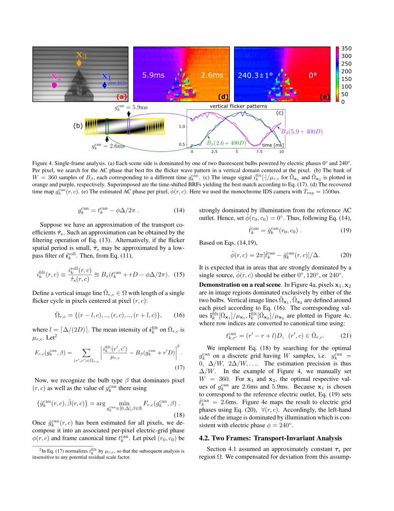
Figure 4. Single-frame analysis. (a) Each scene side is dominated by one of two fluorescent bulbs powered by electric phases 0° and 240°.

Per pixel, we search for the AC phase that best fits the flicker wave pattern in a vertical domain centered at the pixel. (b) The bank of

W = 360 samples of Bβ , each corresponding to a different time gcank . (c) The image signal ifiltk [·]/μr,c for Ωx1 and Ωx2 is plotted in

orange and purple, respectively. Superimposed are the time-shifted BRFs yielding the best match according to Eq. (17). (d) The recovered

time map gcank (r, c). (e) The estimated AC phase per pixel, φ(r, c). Here we used the monochrome IDS camera with Texp = 1500us.

gcank = tcank − φΔ/2π . (14)

Suppose we have an approximation of the transport co-

efficients τs. Such an approximation can be obtained by the

filtering operation of Eq. (13). Alternatively, if the flicker

spatial period is small, τs may be approximated by a low-

pass filter of irollk . Then, from Eq. (11),

ifiltk (r, c) ≡ irollk (r, c)

τs(r, c)� Bs(t

cank + rD − φΔ/2π). (15)

Define a vertical image line Ωr,c ∈ Ωwith length of a single

flicker cycle in pixels centered at pixel (r, c):

Ωr,c = {(r − l, c), .., (r, c), .., (r + l, c)}, (16)

where l = �Δ/(2D)�. The mean intensity of ifiltk on Ωr,c is

μr,c. Let2

Fr,c(gcank , β) =

∑(r′,c′)∈Ωr,c

∣∣∣∣ ifiltk (r′, c′)μr,c

−Bβ(gcank + r′D)

∣∣∣∣2

.

(17)

Now, we recognize the bulb type β that dominates pixel

(r, c) as well as the value of gcank there using

{gcank (r, c), β(r, c)} = arg mingcank ∈[0,Δ],β∈B

Fr,c(gcank , β) .

(18)

Once gcank (r, c) has been estimated for all pixels, we de-

compose it into an associated per-pixel electric-grid phase

φ(r, c) and frame canonical time tcank . Let pixel (r0, c0) be

2In Eq. (17) normalizes ifiltk by μr,c, so that the subsequent analysis is

insensitive to any potential residual scale factor.

strongly dominated by illumination from the reference AC

outlet. Hence, set φ(r0, c0) = 0◦. Thus, following Eq. (14),

tcank = gcank (r0, c0) . (19)

Based on Eqs. (14,19),

φ(r, c) = 2π[tcank − gcank (r, c)]/Δ. (20)

It is expected that in areas that are strongly dominated by a

single source, φ(r, c) should be either 0◦, 120◦, or 240◦.Demonstration on a real scene. In Figure 4a, pixels x1,x2

are in image regions dominated exclusively by either of the

two bulbs. Vertical image lines Ωx1, Ωx2

are defined around

each pixel according to Eq. (16). The corresponding val-

ues ifiltk [Ωx1]/μx1

, ifiltk [Ωx2]/μx2

are plotted in Figure 4c,

where row indices are converted to canonical time using:

tcank,r′ = (r′ − r + l)D, (r′, c) ∈ Ωr,c. (21)

We implement Eq. (18) by searching for the optimal

gcank on a discrete grid having W samples, i.e. gcank =0, Δ/W, 2Δ/W, . . .. The estimation precision is thus

Δ/W . In the example of Figure 4, we manually set

W = 360. For x1 and x2, the optimal respective val-

ues of gcank are 2.6ms and 5.9ms. Because x1 is chosen

to correspond to the reference electric outlet, Eq. (19) sets

tcank = 2.6ms. Figure 4e maps the result to electric grid

phases using Eq. (20), ∀(r, c). Accordingly, the left-hand

side of the image is dominated by illumination which is con-

sistent with electric phase φ = 240◦.

4.2. Two Frames: Transport-Invariant AnalysisSection 4.1 assumed an approximately constant τs per

region Ω. We compensated for deviation from this assump-

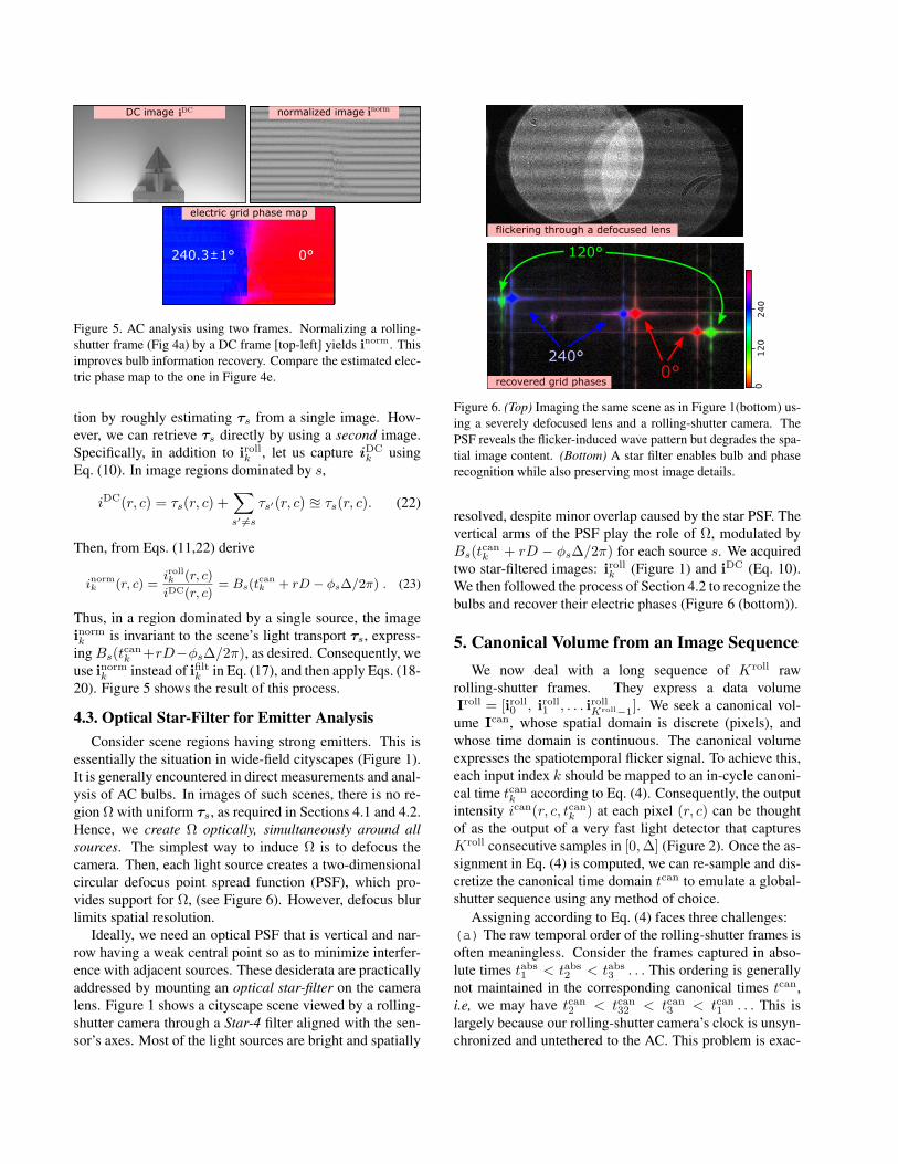
Figure 5. AC analysis using two frames. Normalizing a rolling-

shutter frame (Fig 4a) by a DC frame [top-left] yields inorm. This

improves bulb information recovery. Compare the estimated elec-

tric phase map to the one in Figure 4e.

tion by roughly estimating τs from a single image. How-

ever, we can retrieve τs directly by using a second image.

Specifically, in addition to irollk , let us capture iDCk using

Eq. (10). In image regions dominated by s,

iDC(r, c) = τs(r, c) +∑s′ �=s

τs′(r, c) � τs(r, c). (22)

Then, from Eqs. (11,22) derive

inormk (r, c) =irollk (r, c)

iDC(r, c)= Bs(t

cank + rD − φsΔ/2π) . (23)

Thus, in a region dominated by a single source, the image

inormk is invariant to the scene’s light transport τs, express-ingBs(t

cank +rD−φsΔ/2π), as desired. Consequently, we

use inormk instead of ifiltk in Eq. (17), and then apply Eqs. (18-

20). Figure 5 shows the result of this process.

4.3. Optical Star-Filter for Emitter AnalysisConsider scene regions having strong emitters. This is

essentially the situation in wide-field cityscapes (Figure 1).

It is generally encountered in direct measurements and anal-

ysis of AC bulbs. In images of such scenes, there is no re-

gion Ω with uniform τs, as required in Sections 4.1 and 4.2.

Hence, we create Ω optically, simultaneously around allsources. The simplest way to induce Ω is to defocus the

camera. Then, each light source creates a two-dimensional

circular defocus point spread function (PSF), which pro-

vides support for Ω, (see Figure 6). However, defocus blur

limits spatial resolution.

Ideally, we need an optical PSF that is vertical and nar-

row having a weak central point so as to minimize interfer-

ence with adjacent sources. These desiderata are practically

addressed by mounting an optical star-filter on the camera

lens. Figure 1 shows a cityscape scene viewed by a rolling-

shutter camera through a Star-4 filter aligned with the sen-

sor’s axes. Most of the light sources are bright and spatially

Figure 6. (Top) Imaging the same scene as in Figure 1(bottom) us-

ing a severely defocused lens and a rolling-shutter camera. The

PSF reveals the flicker-induced wave pattern but degrades the spa-

tial image content. (Bottom) A star filter enables bulb and phase

recognition while also preserving most image details.

resolved, despite minor overlap caused by the star PSF. The

vertical arms of the PSF play the role of Ω, modulated by

Bs(tcank + rD − φsΔ/2π) for each source s. We acquired

two star-filtered images: irollk (Figure 1) and iDC (Eq. 10).

We then followed the process of Section 4.2 to recognize the

bulbs and recover their electric phases (Figure 6 (bottom)).

5. Canonical Volume from an Image SequenceWe now deal with a long sequence of Kroll raw

rolling-shutter frames. They express a data volume

Iroll = [iroll0 , iroll1 , . . . irollKroll−1]. We seek a canonical vol-

ume Ican, whose spatial domain is discrete (pixels), and

whose time domain is continuous. The canonical volume

expresses the spatiotemporal flicker signal. To achieve this,

each input index k should be mapped to an in-cycle canoni-

cal time tcank according to Eq. (4). Consequently, the output

intensity ican(r, c, tcank ) at each pixel (r, c) can be thought

of as the output of a very fast light detector that captures

Kroll consecutive samples in [0,Δ] (Figure 2). Once the as-

signment in Eq. (4) is computed, we can re-sample and dis-

cretize the canonical time domain tcan to emulate a global-

shutter sequence using any method of choice.

Assigning according to Eq. (4) faces three challenges:

(a) The raw temporal order of the rolling-shutter frames is

often meaningless. Consider the frames captured in abso-

lute times tabs1 < tabs2 < tabs3 . . . This ordering is generally

not maintained in the corresponding canonical times tcan,i.e, we may have tcan2 < tcan32 < tcan3 < tcan1 . . . This is

largely because our rolling-shutter camera’s clock is unsyn-

chronized and untethered to the AC. This problem is exac-

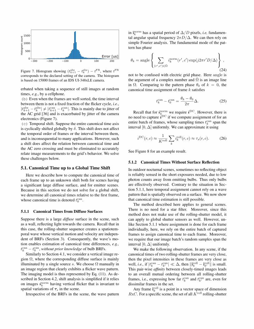
Figure 7. Histogram showing (tabsk+1 − tabsk ) − tFR, where tFR

corresponds to the declared setting of the camera. The histogram

is based on 15000 frames of an IDS UI-348xLE camera.

erbated when taking a sequence of still images at random

times, e.g., by a cellphone.

(b) Even when the frames are well sorted, the time interval

between them is not a fixed fraction of the flicker cycle, i.e.,|tabsk+1− tabsk | = |tcank+1− tcank |. This is mainly due to jitter of

the AC grid [36] and is exacerbated by jitter of the camera

electronics (Figure 7).

(c) Temporal shift. Suppose the entire canonical time axis

is cyclically shifted globally by δ. This shift does not affect

the temporal order of frames or the interval between them,

and is inconsequential to many applications. However, such

a shift does affect the relation between canonical time and

the AC zero crossing and must be eliminated to accurately

relate image measurements to the grid’s behavior. We solve

these challenges below.

5.1. Canonical Time up to a Global Time ShiftHere we describe how to compute the canonical time of

each frame up to an unknown shift both for scenes having

a significant large diffuse surface, and for emitter scenes.

Because in this section we do not solve for a global shift,

we determine all canonical times relative to the first frame,

whose canonical time is denoted tcan0 .

5.1.1 Canonical Times from Diffuse Surfaces

Suppose there is a large diffuse surface in the scene, such

as a wall, reflecting light towards the camera. Recall that in

this case, the rolling-shutter sequence creates a spatiotem-

poral wave whose vertical motion and velocity are indepen-

dent of BRFs (Section 3). Consequently, the wave’s mo-

tion enables estimation of canonical time differences, e.g.,tcank − tcan0 , without prior knowledge of bulb BRFs.

Similarly to Section 4.1, we consider a vertical image re-

gion Ω, where the corresponding diffuse surface is mainly

illuminated by a single source s. We choose Ω manually in

an image region that clearly exhibits a flicker wave pattern.

The imaging model is thus represented by Eq. (11). As de-

scribed in Section 4.2, shift analysis is simplified if it relies

on images inormk having vertical flicker that is invariant to

spatial variations of τs in the scene.

Irrespective of the BRFs in the scene, the wave pattern

in inormk has a spatial period of Δ/D pixels, i.e, fundamen-

tal angular spatial frequency 2πD/Δ. We can then rely on

simple Fourier analysis. The fundamental mode of the pat-

tern has phase

θk = angle

⎧⎨⎩∑

(r′,c′)∈Ω

inormk (r′, c′) exp(j2πr′D/Δ)

⎫⎬⎭ ,

(24)

not to be confused with electric grid phase. Here angle is

the argument of a complex number and Ω is an image line

in Ω. Comparing to the pattern phase θ0 of k = 0, the

canonical time assignment of frame k satisfies

tcank − tcan0 =θk − θ02π

Δ. (25)

Recall that for inormk we require iDC. However, there is

no need to capture iDC if we compute assignment of for an

entire batch of frames, whose sampling times tcank span the

interval [0,Δ] uniformly. We can approximate it using

iDC(r, c) ≈ 1

Kroll

∑k

irollk (r, c) ≈ τs(r, c). (26)

See Figure 8 for an example result.

5.1.2 Canonical Times Without Surface Reflection

In outdoor nocturnal scenes, sometimes no reflecting object

is reliably sensed in the short exposures needed, due to low

photon counts away from emitting bulbs. Thus only bulbs

are effectively observed. Contrary to the situation in Sec-

tion 5.1.1, here temporal assignment cannot rely on a wave

pattern that is spatially observed on a surface. We now show

that canonical time estimation is still possible.

The method described here applies to general scenes.

There is no need for a star filter. Moreover, since this

method does not make use of the rolling-shutter model, it

can apply to global shutter sensors as well. However, un-

like Section 5.1.1 where assignment is done for each frame

individually, here, we rely on the entire batch of captured

frames to assign canonical time to each frame. Moreover,

we require that our image batch’s random samples span the

interval [0,Δ] uniformly.

We make the following observation. In any scene, if the

canonical times of two rolling-shutter frames are very close,

then the pixel intensities in these frames are very close as

well, i.e., if |tcank − tcank′ | � Δ, then ‖irollk − irollk′ ‖ is small.

This pair-wise affinity between closely-timed images leads

to an overall mutual ordering between all rolling-shutter

frames, i.e., expressing how far tcank and tcank′ are, even for

dissimilar frames in the set.

Any frame irollk is a point in a vector space of dimension

RxC. For a specific scene, the set of allKroll rolling-shutter

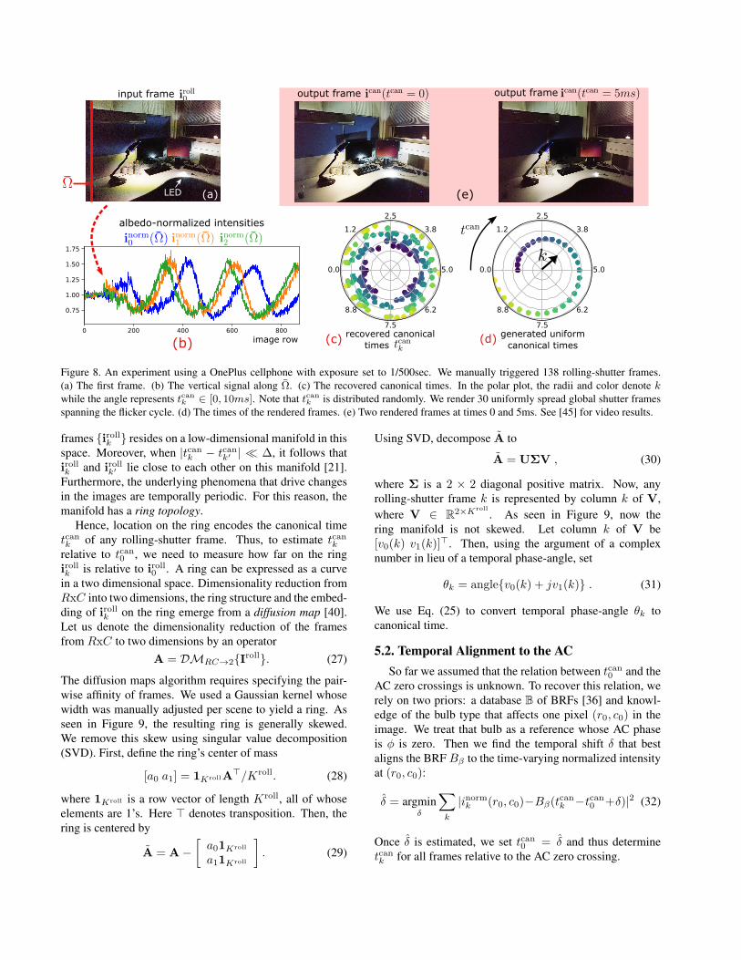
Figure 8. An experiment using a OnePlus cellphone with exposure set to 1/500sec. We manually triggered 138 rolling-shutter frames.

(a) The first frame. (b) The vertical signal along Ω. (c) The recovered canonical times. In the polar plot, the radii and color denote kwhile the angle represents tcank ∈ [0, 10ms]. Note that tcank is distributed randomly. We render 30 uniformly spread global shutter frames

spanning the flicker cycle. (d) The times of the rendered frames. (e) Two rendered frames at times 0 and 5ms. See [45] for video results.

frames {irollk } resides on a low-dimensional manifold in this

space. Moreover, when |tcank − tcank′ | � Δ, it follows that

irollk and irollk′ lie close to each other on this manifold [21].

Furthermore, the underlying phenomena that drive changes

in the images are temporally periodic. For this reason, the

manifold has a ring topology.Hence, location on the ring encodes the canonical time

tcank of any rolling-shutter frame. Thus, to estimate tcank

relative to tcan0 , we need to measure how far on the ring

irollk is relative to iroll0 . A ring can be expressed as a curve

in a two dimensional space. Dimensionality reduction from

RxC into two dimensions, the ring structure and the embed-

ding of irollk on the ring emerge from a diffusion map [40].

Let us denote the dimensionality reduction of the frames

from RxC to two dimensions by an operator

A = DMRC→2{Iroll}. (27)

The diffusion maps algorithm requires specifying the pair-

wise affinity of frames. We used a Gaussian kernel whose

width was manually adjusted per scene to yield a ring. As

seen in Figure 9, the resulting ring is generally skewed.

We remove this skew using singular value decomposition

(SVD). First, define the ring’s center of mass

[a0 a1] = 1KrollA�/Kroll. (28)

where 1Kroll is a row vector of length Kroll, all of whose

elements are 1’s. Here � denotes transposition. Then, the

ring is centered by

A = A−[a01Kroll

a11Kroll

]. (29)

Using SVD, decompose A to

A = UΣV , (30)

where Σ is a 2 × 2 diagonal positive matrix. Now, any

rolling-shutter frame k is represented by column k of V,

where V ∈ R2×Kroll

. As seen in Figure 9, now the

ring manifold is not skewed. Let column k of V be

[v0(k) v1(k)]�. Then, using the argument of a complex

number in lieu of a temporal phase-angle, set

θk = angle{v0(k) + jv1(k)} . (31)

We use Eq. (25) to convert temporal phase-angle θk to

canonical time.

5.2. Temporal Alignment to the ACSo far we assumed that the relation between tcan0 and the

AC zero crossings is unknown. To recover this relation, we

rely on two priors: a database B of BRFs [36] and knowl-

edge of the bulb type that affects one pixel (r0, c0) in the

image. We treat that bulb as a reference whose AC phase

is φ is zero. Then we find the temporal shift δ that best

aligns the BRF Bβ to the time-varying normalized intensity

at (r0, c0):

δ = argminδ

∑k

|inormk (r0, c0)−Bβ(tcank −tcan0 +δ)|2 (32)

Once δ is estimated, we set tcan0 = δ and thus determine

tcank for all frames relative to the AC zero crossing.

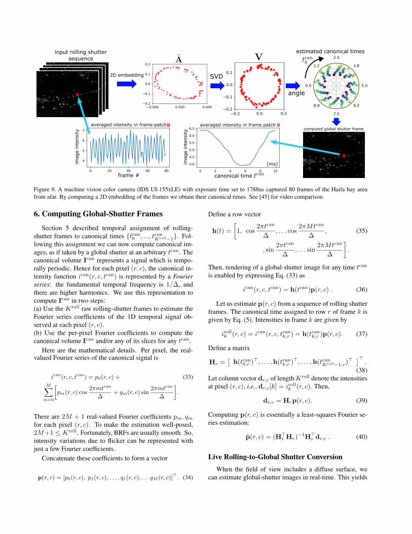
Figure 9. A machine vision color camera (IDS UI-155xLE) with exposure time set to 1788us captured 80 frames of the Haifa bay area

from afar. By computing a 2D embedding of the frames we obtain their canonical times. See [45] for video comparison.

6. Computing Global-Shutter Frames

Section 5 described temporal assignment of rolling-

shutter frames to canonical times {tcan0 , ..., tcanKroll−1}. Fol-

lowing this assignment we can now compute canonical im-

ages, as if taken by a global shutter at an arbitrary tcan. The

canonical volume Ican represents a signal which is tempo-

rally periodic. Hence for each pixel (r, c), the canonical in-

tensity function ican(r, c, tcan) is represented by a Fourierseries: the fundamental temporal frequency is 1/Δ, and

there are higher harmonics. We use this representation to

compute Ican in two steps:

(a) Use the Kroll raw rolling-shutter frames to estimate the

Fourier series coefficients of the 1D temporal signal ob-

served at each pixel (r, c).(b) Use the per-pixel Fourier coefficients to compute the

canonical volume Ican and/or any of its slices for any tcan.

Here are the mathematical details. Per pixel, the real-valued Fourier series of the canonical signal is

ican(r, c, tcan) = p0(r, c) + (33)

M∑m=0

[pm(r, c) cos

2πmtcan

Δ+ qm(r, c) sin

2πmtcan

Δ

].

There are 2M + 1 real-valued Fourier coefficients pm, qmfor each pixel (r, c). To make the estimation well-posed,

2M+1 ≤ Kroll. Fortunately, BRFs are usually smooth. So,

intensity variations due to flicker can be represented with

just a few Fourier coefficients.

Concatenate these coefficients to form a vector

p(r, c) = [p0(r, c), p1(r, c), . . . , q1(r, c), . . . qM (r, c)]�. (34)

Define a row vector

h(t) =

[1, cos

2πtcan

Δ, . . . cos

2πMtcan

Δ, (35)

, sin2πtcan

Δ, . . . sin

2πMtcan

Δ

].

Then, rendering of a global-shutter image for any time tcan

is enabled by expressing Eq. (33) as

ican(r, c, tcan) = h(tcan)p(r, c) . (36)

Let us estimate p(r, c) from a sequence of rolling shutter

frames. The canonical time assigned to row r of frame k is

given by Eq. (5). Intensities in frame k are given by

irollk (r, c) = ican(r, c, tcank,r ) = h(tcank,r )p(r, c). (37)

Define a matrix

Hr =[h(tcan0,r )

�, . . . ,h(tcank,r )�, . . . ,h(tcanKroll−1,r)

� ]� .(38)

Let column vector dr,c of lengthKroll denote the intensities

at pixel (r, c), i.e., dr,c[k] = irollk (r, c). Then,

dr,c = Hrp(r, c). (39)

Computing p(r, c) is essentially a least-squares Fourier se-

ries estimation:

p(r, c) = (H�r Hr)

−1H�r dr,c . (40)

Live Rolling-to-Global Shutter Conversion

When the field of view includes a diffuse surface, we

can estimate global-shutter images in real-time. This yields

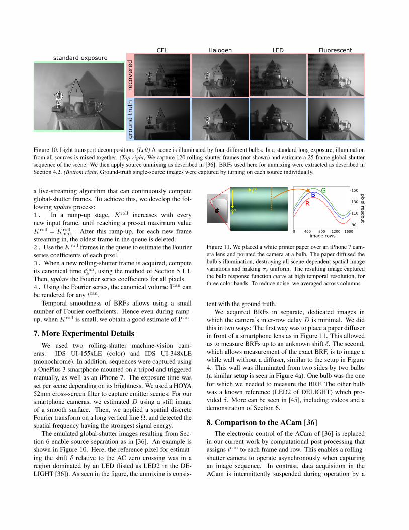
Figure 10. Light transport decomposition. (Left) A scene is illuminated by four different bulbs. In a standard long exposure, illumination

from all sources is mixed together. (Top right) We capture 120 rolling-shutter frames (not shown) and estimate a 25-frame global-shutter

sequence of the scene. We then apply source unmixing as described in [36]. BRFs used here for unmixing were extracted as described in

Section 4.2. (Bottom right) Ground-truth single-source images were captured by turning on each source individually.

a live-streaming algorithm that can continuously compute

global-shutter frames. To achieve this, we develop the fol-

lowing update process:

1. In a ramp-up stage, Kroll increases with every

new input frame, until reaching a pre-set maximum value

Kroll = Krollmax. After this ramp-up, for each new frame

streaming in, the oldest frame in the queue is deleted.

2. Use theKroll frames in the queue to estimate the Fourier

series coefficients of each pixel.

3. When a new rolling-shutter frame is acquired, compute

its canonical time tcank , using the method of Section 5.1.1.

Then, update the Fourier series coefficients for all pixels.

4. Using the Fourier series, the canonical volume Ican can

be rendered for any tcan.Temporal smoothness of BRFs allows using a small

number of Fourier coefficients. Hence even during ramp-

up, whenKroll is small, we obtain a good estimate of Ican.

7. More Experimental DetailsWe used two rolling-shutter machine-vision cam-

eras: IDS UI-155xLE (color) and IDS UI-348xLE

(monochrome). In addition, sequences were captured using

a OnePlus 3 smartphone mounted on a tripod and triggered

manually, as well as an iPhone 7. The exposure time was

set per scene depending on its brightness. We used a HOYA

52mm cross-screen filter to capture emitter scenes. For our

smartphone cameras, we estimated D using a still image

of a smooth surface. Then, we applied a spatial discrete

Fourier transform on a long vertical line Ω, and detected the

spatial frequency having the strongest signal energy.

The emulated global-shutter images resulting from Sec-

tion 6 enable source separation as in [36]. An example is

shown in Figure 10. Here, the reference pixel for estimat-

ing the shift δ relative to the AC zero crossing was in a

region dominated by an LED (listed as LED2 in the DE-

LIGHT [36]). As seen in the figure, the unmixing is consis-

Figure 11. We placed a white printer paper over an iPhone 7 cam-

era lens and pointed the camera at a bulb. The paper diffused the

bulb’s illumination, destroying all scene-dependent spatial image

variations and making τs uniform. The resulting image captured

the bulb response function curve at high temporal resolution, for

three color bands. To reduce noise, we averaged across columns.

tent with the ground truth.

We acquired BRFs in separate, dedicated images in

which the camera’s inter-row delay D is minimal. We did

this in two ways: The first way was to place a paper diffuser

in front of a smartphone lens as in Figure 11. This allowed

us to measure BRFs up to an unknown shift δ. The second,

which allows measurement of the exact BRF, is to image a

while wall without a diffuser, similar to the setup in Figure

4. This wall was illuminated from two sides by two bulbs

(a similar setup is seen in Figure 4a). One bulb was the one

for which we needed to measure the BRF. The other bulb

was a known reference (LED2 of DELIGHT) which pro-

vided δ. More can be seen in [45], including videos and a

demonstration of Section 6.

8. Comparison to the ACam [36]The electronic control of the ACam of [36] is replaced

in our current work by computational post processing that

assigns tcan to each frame and row. This enables a rolling-

shutter camera to operate asynchronously when capturing

an image sequence. In contrast, data acquisition in the

ACam is intermittently suspended during operation by a

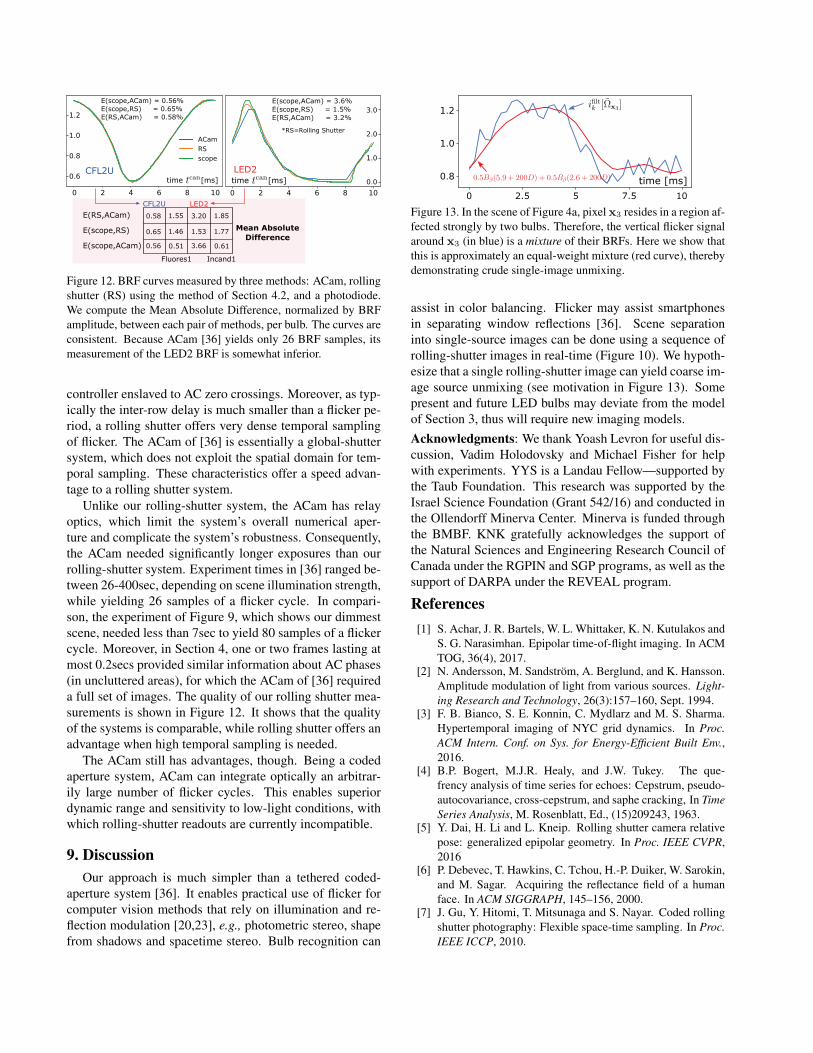
Figure 12. BRF curves measured by three methods: ACam, rolling

shutter (RS) using the method of Section 4.2, and a photodiode.

We compute the Mean Absolute Difference, normalized by BRF

amplitude, between each pair of methods, per bulb. The curves are

consistent. Because ACam [36] yields only 26 BRF samples, its

measurement of the LED2 BRF is somewhat inferior.

controller enslaved to AC zero crossings. Moreover, as typ-

ically the inter-row delay is much smaller than a flicker pe-

riod, a rolling shutter offers very dense temporal sampling

of flicker. The ACam of [36] is essentially a global-shutter

system, which does not exploit the spatial domain for tem-

poral sampling. These characteristics offer a speed advan-

tage to a rolling shutter system.

Unlike our rolling-shutter system, the ACam has relay

optics, which limit the system’s overall numerical aper-

ture and complicate the system’s robustness. Consequently,

the ACam needed significantly longer exposures than our

rolling-shutter system. Experiment times in [36] ranged be-

tween 26-400sec, depending on scene illumination strength,

while yielding 26 samples of a flicker cycle. In compari-

son, the experiment of Figure 9, which shows our dimmest

scene, needed less than 7sec to yield 80 samples of a flicker

cycle. Moreover, in Section 4, one or two frames lasting at

most 0.2secs provided similar information about AC phases

(in uncluttered areas), for which the ACam of [36] required

a full set of images. The quality of our rolling shutter mea-

surements is shown in Figure 12. It shows that the quality

of the systems is comparable, while rolling shutter offers an

advantage when high temporal sampling is needed.

The ACam still has advantages, though. Being a coded

aperture system, ACam can integrate optically an arbitrar-

ily large number of flicker cycles. This enables superior

dynamic range and sensitivity to low-light conditions, with

which rolling-shutter readouts are currently incompatible.

9. DiscussionOur approach is much simpler than a tethered coded-

aperture system [36]. It enables practical use of flicker for

computer vision methods that rely on illumination and re-

flection modulation [20,23], e.g., photometric stereo, shape

from shadows and spacetime stereo. Bulb recognition can

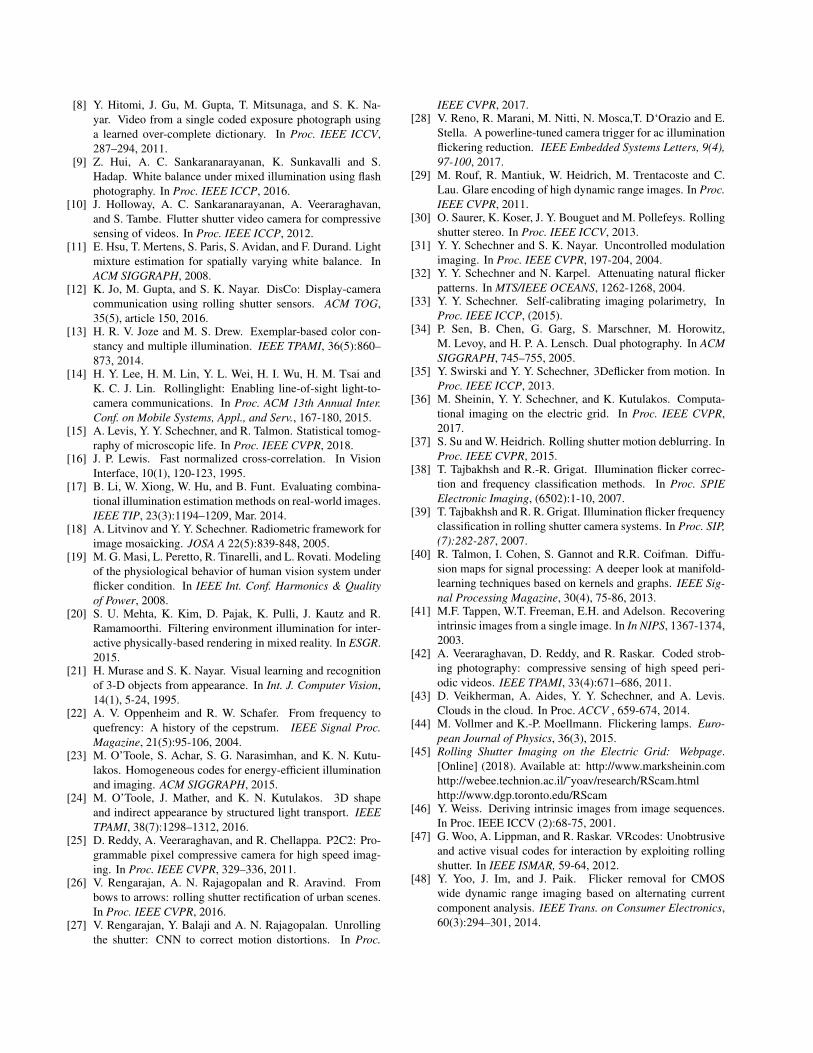
Figure 13. In the scene of Figure 4a, pixel x3 resides in a region af-

fected strongly by two bulbs. Therefore, the vertical flicker signal

around x3 (in blue) is a mixture of their BRFs. Here we show that

this is approximately an equal-weight mixture (red curve), thereby

demonstrating crude single-image unmixing.

assist in color balancing. Flicker may assist smartphones

in separating window reflections [36]. Scene separation

into single-source images can be done using a sequence of

rolling-shutter images in real-time (Figure 10). We hypoth-

esize that a single rolling-shutter image can yield coarse im-

age source unmixing (see motivation in Figure 13). Some

present and future LED bulbs may deviate from the model

of Section 3, thus will require new imaging models.

Acknowledgments: We thank Yoash Levron for useful dis-

cussion, Vadim Holodovsky and Michael Fisher for help

with experiments. YYS is a Landau Fellow—supported by

the Taub Foundation. This research was supported by the

Israel Science Foundation (Grant 542/16) and conducted in

the Ollendorff Minerva Center. Minerva is funded through

the BMBF. KNK gratefully acknowledges the support of

the Natural Sciences and Engineering Research Council of

Canada under the RGPIN and SGP programs, as well as the

support of DARPA under the REVEAL program.

References[1] S. Achar, J. R. Bartels, W. L. Whittaker, K. N. Kutulakos and

S. G. Narasimhan. Epipolar time-of-flight imaging. In ACM

TOG, 36(4), 2017.[2] N. Andersson, M. Sandstrom, A. Berglund, and K. Hansson.

Amplitude modulation of light from various sources. Light-ing Research and Technology, 26(3):157–160, Sept. 1994.

[3] F. B. Bianco, S. E. Konnin, C. Mydlarz and M. S. Sharma.

Hypertemporal imaging of NYC grid dynamics. In Proc.ACM Intern. Conf. on Sys. for Energy-Efficient Built Env.,2016.

[4] B.P. Bogert, M.J.R. Healy, and J.W. Tukey. The que-

frency analysis of time series for echoes: Cepstrum, pseudo-

autocovariance, cross-cepstrum, and saphe cracking, In TimeSeries Analysis, M. Rosenblatt, Ed., (15)209243, 1963.

[5] Y. Dai, H. Li and L. Kneip. Rolling shutter camera relative

pose: generalized epipolar geometry. In Proc. IEEE CVPR,

2016[6] P. Debevec, T. Hawkins, C. Tchou, H.-P. Duiker, W. Sarokin,

and M. Sagar. Acquiring the reflectance field of a human

face. In ACM SIGGRAPH, 145–156, 2000.[7] J. Gu, Y. Hitomi, T. Mitsunaga and S. Nayar. Coded rolling

shutter photography: Flexible space-time sampling. In Proc.IEEE ICCP, 2010.

[8] Y. Hitomi, J. Gu, M. Gupta, T. Mitsunaga, and S. K. Na-

yar. Video from a single coded exposure photograph using

a learned over-complete dictionary. In Proc. IEEE ICCV,

287–294, 2011.[9] Z. Hui, A. C. Sankaranarayanan, K. Sunkavalli and S.

Hadap. White balance under mixed illumination using flash

photography. In Proc. IEEE ICCP, 2016.[10] J. Holloway, A. C. Sankaranarayanan, A. Veeraraghavan,

and S. Tambe. Flutter shutter video camera for compressive

sensing of videos. In Proc. IEEE ICCP, 2012.[11] E. Hsu, T. Mertens, S. Paris, S. Avidan, and F. Durand. Light

mixture estimation for spatially varying white balance. In

ACM SIGGRAPH, 2008.[12] K. Jo, M. Gupta, and S. K. Nayar. DisCo: Display-camera

communication using rolling shutter sensors. ACM TOG,

35(5), article 150, 2016.[13] H. R. V. Joze and M. S. Drew. Exemplar-based color con-

stancy and multiple illumination. IEEE TPAMI, 36(5):860–873, 2014.

[14] H. Y. Lee, H. M. Lin, Y. L. Wei, H. I. Wu, H. M. Tsai and

K. C. J. Lin. Rollinglight: Enabling line-of-sight light-to-

camera communications. In Proc. ACM 13th Annual Inter.Conf. on Mobile Systems, Appl., and Serv., 167-180, 2015.

[15] A. Levis, Y. Y. Schechner, and R. Talmon. Statistical tomog-

raphy of microscopic life. In Proc. IEEE CVPR, 2018.[16] J. P. Lewis. Fast normalized cross-correlation. In Vision

Interface, 10(1), 120-123, 1995.[17] B. Li, W. Xiong, W. Hu, and B. Funt. Evaluating combina-

tional illumination estimation methods on real-world images.

IEEE TIP, 23(3):1194–1209, Mar. 2014.[18] A. Litvinov and Y. Y. Schechner. Radiometric framework for

image mosaicking. JOSA A 22(5):839-848, 2005.[19] M. G. Masi, L. Peretto, R. Tinarelli, and L. Rovati. Modeling

of the physiological behavior of human vision system under

flicker condition. In IEEE Int. Conf. Harmonics & Qualityof Power, 2008.

[20] S. U. Mehta, K. Kim, D. Pajak, K. Pulli, J. Kautz and R.

Ramamoorthi. Filtering environment illumination for inter-

active physically-based rendering in mixed reality. In ESGR.

2015.[21] H. Murase and S. K. Nayar. Visual learning and recognition

of 3-D objects from appearance. In Int. J. Computer Vision,14(1), 5-24, 1995.

[22] A. V. Oppenheim and R. W. Schafer. From frequency to

quefrency: A history of the cepstrum. IEEE Signal Proc.Magazine, 21(5):95-106, 2004.

[23] M. O’Toole, S. Achar, S. G. Narasimhan, and K. N. Kutu-

lakos. Homogeneous codes for energy-efficient illumination

and imaging. ACM SIGGRAPH, 2015.[24] M. O’Toole, J. Mather, and K. N. Kutulakos. 3D shape

and indirect appearance by structured light transport. IEEETPAMI, 38(7):1298–1312, 2016.

[25] D. Reddy, A. Veeraraghavan, and R. Chellappa. P2C2: Pro-

grammable pixel compressive camera for high speed imag-

ing. In Proc. IEEE CVPR, 329–336, 2011.[26] V. Rengarajan, A. N. Rajagopalan and R. Aravind. From

bows to arrows: rolling shutter rectification of urban scenes.

In Proc. IEEE CVPR, 2016.[27] V. Rengarajan, Y. Balaji and A. N. Rajagopalan. Unrolling

the shutter: CNN to correct motion distortions. In Proc.

IEEE CVPR, 2017.[28] V. Reno, R. Marani, M. Nitti, N. Mosca,T. D‘Orazio and E.

Stella. A powerline-tuned camera trigger for ac illumination

flickering reduction. IEEE Embedded Systems Letters, 9(4),97-100, 2017.

[29] M. Rouf, R. Mantiuk, W. Heidrich, M. Trentacoste and C.

Lau. Glare encoding of high dynamic range images. In Proc.IEEE CVPR, 2011.

[30] O. Saurer, K. Koser, J. Y. Bouguet and M. Pollefeys. Rolling

shutter stereo. In Proc. IEEE ICCV, 2013.[31] Y. Y. Schechner and S. K. Nayar. Uncontrolled modulation

imaging. In Proc. IEEE CVPR, 197-204, 2004.[32] Y. Y. Schechner and N. Karpel. Attenuating natural flicker

patterns. In MTS/IEEE OCEANS, 1262-1268, 2004.[33] Y. Y. Schechner. Self-calibrating imaging polarimetry, In

Proc. IEEE ICCP, (2015).[34] P. Sen, B. Chen, G. Garg, S. Marschner, M. Horowitz,

M. Levoy, and H. P. A. Lensch. Dual photography. In ACMSIGGRAPH, 745–755, 2005.

[35] Y. Swirski and Y. Y. Schechner, 3Deflicker from motion. In

Proc. IEEE ICCP, 2013.[36] M. Sheinin, Y. Y. Schechner, and K. Kutulakos. Computa-

tional imaging on the electric grid. In Proc. IEEE CVPR,

2017.[37] S. Su and W. Heidrich. Rolling shutter motion deblurring. In

Proc. IEEE CVPR, 2015.[38] T. Tajbakhsh and R.-R. Grigat. Illumination flicker correc-

tion and frequency classification methods. In Proc. SPIEElectronic Imaging, (6502):1-10, 2007.

[39] T. Tajbakhsh and R. R. Grigat. Illumination flicker frequency

classification in rolling shutter camera systems. In Proc. SIP,(7):282-287, 2007.

[40] R. Talmon, I. Cohen, S. Gannot and R.R. Coifman. Diffu-

sion maps for signal processing: A deeper look at manifold-

learning techniques based on kernels and graphs. IEEE Sig-nal Processing Magazine, 30(4), 75-86, 2013.

[41] M.F. Tappen, W.T. Freeman, E.H. and Adelson. Recovering

intrinsic images from a single image. In In NIPS, 1367-1374,2003.

[42] A. Veeraraghavan, D. Reddy, and R. Raskar. Coded strob-

ing photography: compressive sensing of high speed peri-

odic videos. IEEE TPAMI, 33(4):671–686, 2011.[43] D. Veikherman, A. Aides, Y. Y. Schechner, and A. Levis.

Clouds in the cloud. In Proc. ACCV , 659-674, 2014.[44] M. Vollmer and K.-P. Moellmann. Flickering lamps. Euro-

pean Journal of Physics, 36(3), 2015.[45] Rolling Shutter Imaging on the Electric Grid: Webpage.

[Online] (2018). Available at: http://www.marksheinin.com

http://webee.technion.ac.il/˜yoav/research/RScam.html

http://www.dgp.toronto.edu/RScam[46] Y. Weiss. Deriving intrinsic images from image sequences.

In Proc. IEEE ICCV (2):68-75, 2001.[47] G. Woo, A. Lippman, and R. Raskar. VRcodes: Unobtrusive

and active visual codes for interaction by exploiting rolling

shutter. In IEEE ISMAR, 59-64, 2012.[48] Y. Yoo, J. Im, and J. Paik. Flicker removal for CMOS

wide dynamic range imaging based on alternating current

component analysis. IEEE Trans. on Consumer Electronics,60(3):294–301, 2014.