Rolling Radius - Luis Arimany | La Web de Luis Arimany€¦ · Web view · 2015-05-25B.1.1-Description of the experiment. The inertia of the wheel about its spin axis is determined

Vehicle Dynamics Assignment: Frequency response to steering angle input

3. GROUP B

PARAMETERS MEASUREMENT PARAMETERS MEASUREMENT

IN THE IN THE FORD MONDEOFORD MONDEO

www.luisarimany.com Group B; Parameters Measurement83

Ford Mondeo used to perform the parameters measurements.Cranfield’s Airfield. First day of testing. 5:45 a.m.

Cranfield’s Airfield. First day of testing. 5:45 a.m.

http://www.luisarimany.com/


B.1-MEASUREMENT OF THE WHEEL INERTIA ABOUT ITS SPIN AXIS

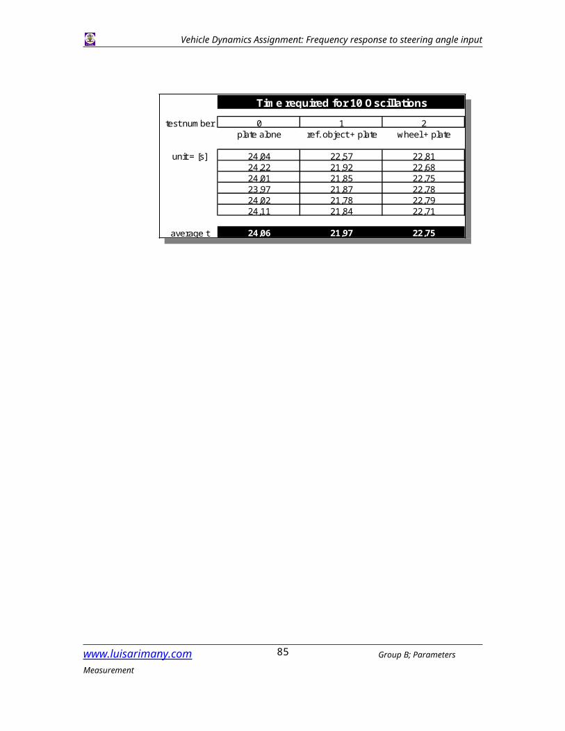
B.1.1-Description of the experimentThe inertia of the wheel about its spin axis is determined by using a testing device called the “trifilar suspension”. It consits of a wooden plate circular platform with a radius R = 0.3m and a mass of 4kg. The plateform is supported by 3 wires of equal length L = 2.20m (see photograph).3 series of tests will allow us to determine the inertia of the wheel by comparing the oscilation periods of the system:- With the plate alone- With the wheel put on the plate- With a reference object put on the plate.We measure the time required for 10 free oscillations of the system in the 3 different configurations explained previously.

B.1.2-Data, Formula and Results Data


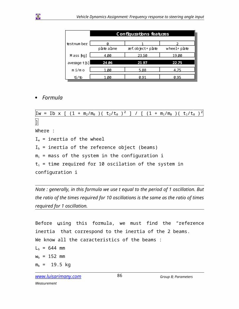
test number 0 1 2plate alone ref. object + plate wheel + plate

unit = [s] 24,04 22,57 22,8124,22 21,92 22,6824,01 21,85 22,7523,97 21,87 22,7824,02 21,78 22,7924,11 21,84 22,71

average t 24,06 21,97 22,75

Time required for 10 Oscillations



Formula

Iw = Ib x [ (1 + m2/m0 )( t2/t0 )² ] / [ (1 + m1/m0 )( t1/t0 )² ]Where :Iw = inertia of the wheelIb = inertia of the reference object (beams)mi = mass of the system in the configuration iti = time required for 10 oscilation of the system in configuration i

Note : generally, in this formula we use t equal to the period of 1 oscillation. But the ratio of the times required for 10 oscillations is the same as the ratio of times required for 1 oscillation.

Before using this formula, we must find the “reference inertia” that correspond to the inertia of the 2 beams.We know all the caracteristics of the beams :Lb = 644 mmwb = 152 mmmb = 19.5 kgHence we can use the formula :Ib = mb/3 [ Lb²/4 + wb²/4 ]

Results

NA : Ib = 0.7115 km²Thus :

Iw = 0.635 kgm²


test number 0 1 2plate alone ref. object + plate wheel + plate

Mass [kg] 4,00 23,50 19,00

average t [s] 24,06 21,97 22,75

mi / mo 1,00 5,88 4,75

ti / to 1,00 0,91 0,95

Configurations features



B.2-REPARTITION OF THE WEIGHT ON THE WHEEL AXIS

The aim of this measure is to determine the loads (or weights) that are applied on each wheel. These loads must take in account two cases : when the car is unladen and when the car is laden.

B.2.1-Settings

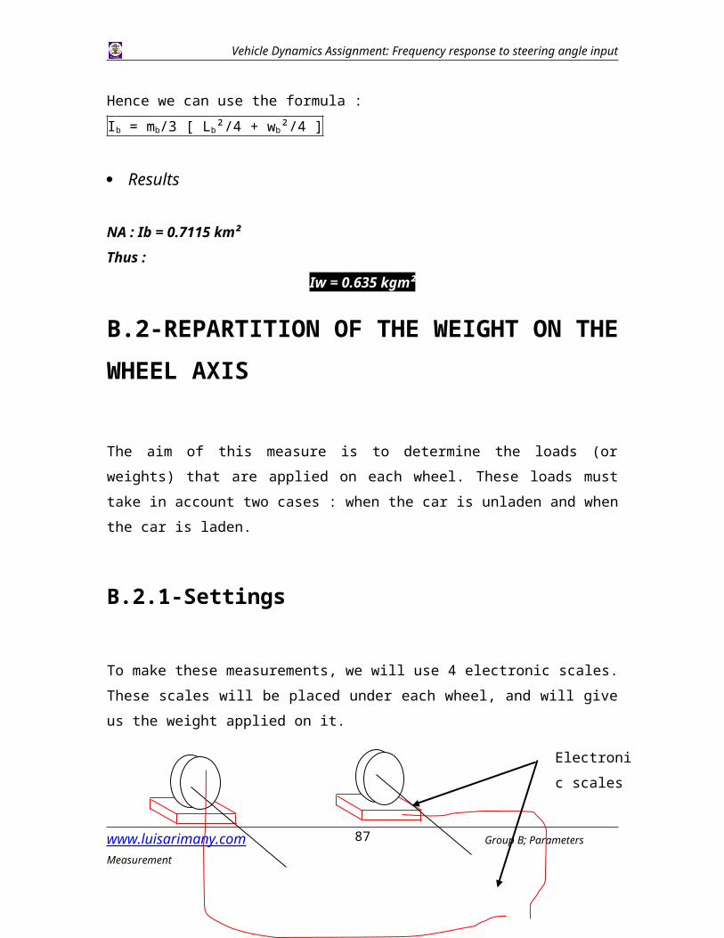
To make these measurements, we will use 4 electronic scales. These scales will be placed under each wheel, and will give us the weight applied on it.

This picture is a shematic view of the setting.

B.2.2-Electronic scales

After having decided what we will do, we have look at the electronic scales. Indeed we wanted to know if the weight they give us were right. For that we have used some heavy thugs (steel plate, people…) we found in the laboratory. First we take their weights with a classical scale, and after we measure it again with the electronic scales.


Electronic scales



We found then that only three of them were in use. Indeed one scale do not work at all. The three other ones were perfect, for weight up to 900 lbs (about 407 kg), which will be sufficient for the measure we have to do.

B.2.3-Measurements

Now we will see what we have done. The fact that only three of the electronic scales work have complicated a little bit our measurement. Indeed for each case (laden and unladen), we had to make twice the measurement. Between the two measurement, we have had to switch the scale which do not work with another one. Hence we had to jack up the car twice instead of one for each measurement. But we succeeded in obtaining results, that are :

Unladen case :

Wheel Front Right Front left Rear Right Rear LeftWeight (in kg) 400 415 256.5 260

Total weight of the car : 1331.5 kg

Laden case :

Wheel Front Right Front left Rear Right Rear LeftWeight (in kg) 455.5 466 405.5 418.5

Total weight of the car : 1745.5 kg

The laden case was obtained by putting two men on the front seats, two on the rear seats and weights (about 80 kg) into the case.




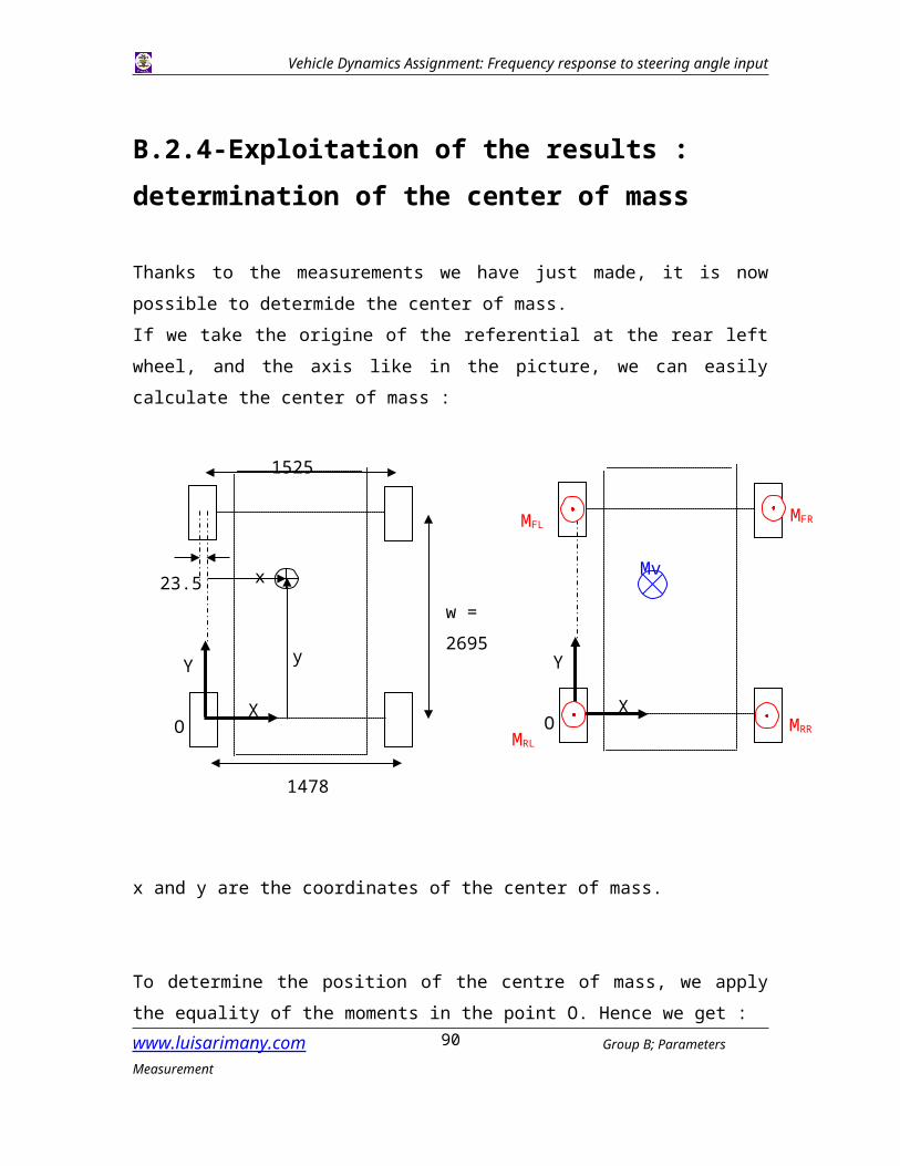
B.2.4-Exploitation of the results : determination of the center of mass

Thanks to the measurements we have just made, it is now possible to determide the center of mass.If we take the origine of the referential at the rear left wheel, and the axis like in the picture, we can easily calculate the center of mass :

x and y are the coordinates of the center of mass.

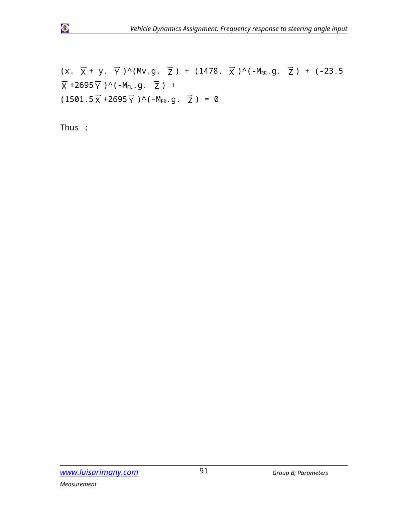
To determine the position of the centre of mass, we apply the equality of the moments in the point O. Hence we get :

(x. + y. )^(Mv.g. ) + (1478. )^(-MRR.g. ) + (-23.5 +2695 )^(-MFL.g. ) + (1501.5 +2695 )^(-MFR.g. ) = 0

Thus :


w = 2695

Y

XO

23.5

1525

1478

x

y Y

XO

Mv

MRR

MFRMFL

MRL



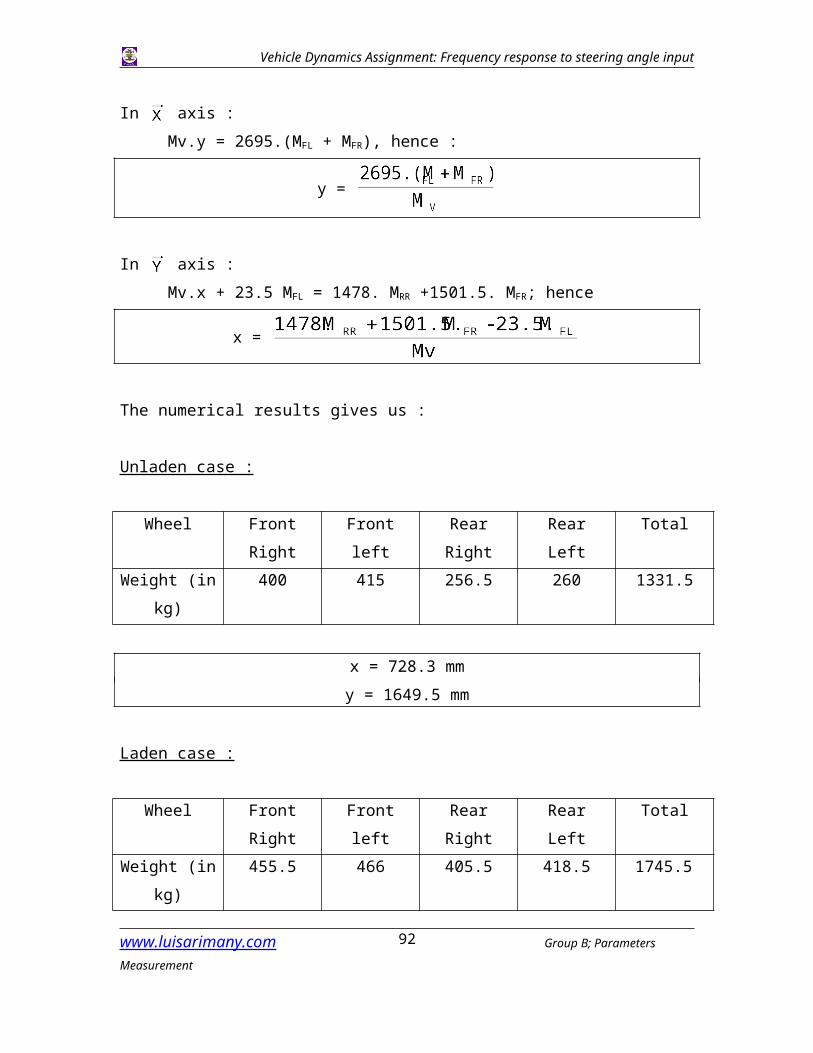
In axis :Mv.y = 2695.(MFL + MFR), hence :

y =

In axis :Mv.x + 23.5 MFL = 1478. MRR +1501.5. MFR; hence

x =

The numerical results gives us :

Unladen case :

Wheel Front Right Front left Rear Right Rear Left TotalWeight (in kg) 400 415 256.5 260 1331.5

x = 728.3 mmy = 1649.5 mm

Laden case :

Wheel Front Right Front left Rear Right Rear Left TotalWeight (in kg) 455.5 466 405.5 418.5 1745.5

x = 728.9 mmy = 1422.8 mm

Hence we can see that the center of mass is near the Y symmetry axis, in the side of the driver, and more towards the front of the car.In the laden case, we can notice that the x position of the center of mass do not vary a lot (less than 1 mm), but the C.O.G is "pushed" towards the rear of the car.We can conclude that the C.O.G is not static, but vary considering the position and the number of passangers, and the luggage for instance.




B.3-Rolling RadiusB.3.1-IntroductionThe rolling radius of a tyre is the effective radius of the tyre when it is mounted and

rotating on a vehicle. It is defined as the translational velocity of the wheel axis divided

by the wheel angular speed:

B.3.2-MethodTo measure the rolling radius of the tyres on the Ford Mondeo the following procedure

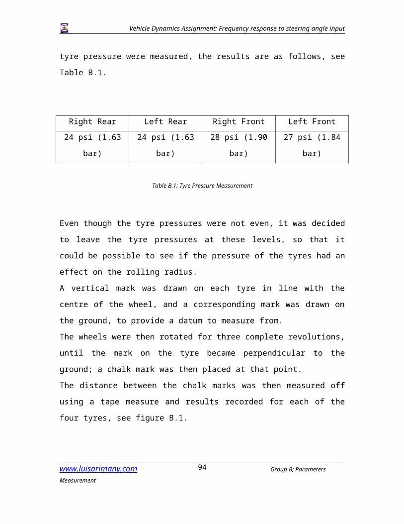
was used. First of all, the tyre pressure were measured, the results are as follows, see

Table B.1.

Right Rear Left Rear Right Front Left Front

24 psi (1.63 bar) 24 psi (1.63 bar) 28 psi (1.90 bar) 27 psi (1.84 bar)

Table B.1: Tyre Pressure Measurement

Even though the tyre pressures were not even, it was decided to leave the tyre pressures

at these levels, so that it could be possible to see if the pressure of the tyres had an effect

on the rolling radius.

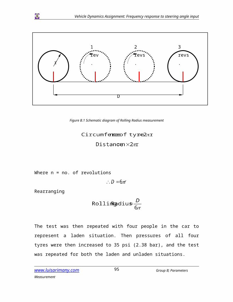
A vertical mark was drawn on each tyre in line with the centre of the wheel, and a

corresponding mark was drawn on the ground, to provide a datum to measure from.

The wheels were then rotated for three complete revolutions, until the mark on the tyre

became perpendicular to the ground; a chalk mark was then placed at that point.

The distance between the chalk marks was then measured off using a tape measure and

results recorded for each of the four tyres, see figure B.1.




Figure B.1 Schematic diagram of Rolling Radius measurement

Where n = no. of revolutions

Rearranging

The test was then repeated with four people in the car to represent a laden situation. Then

pressures of all four tyres were then increased to 35 psi (2.38 bar), and the test was

repeated for both the laden and unladen situations.

Unfortunately when the test was carried out the car had a flat battery, so it was necessary

for several members of the group to push the car, to complete the three revolutions.

Towards the end of the test it was found that the chalk marks on the tyres were not

finishing vertical to the ground.


r

D

1 rev.

2 revs.

3 revs.



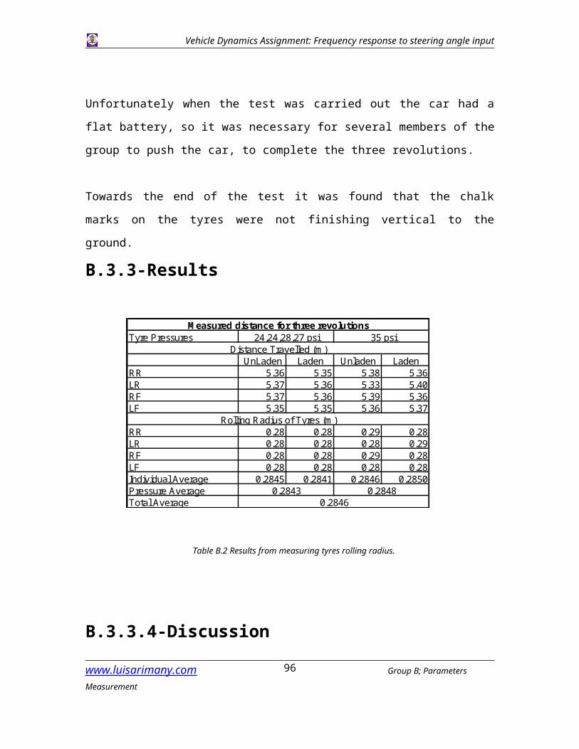
B.3.3-Results

Table B.2 Results from measuring tyres rolling radius.

B.3.3.4-DiscussionUsing the chalk marks and a tape measure, was perhaps not the most accurate way of

measuring the covered distance; but it was hoped that covering three revolutions would

compensate for this problem.

But as you can see from the results above there is negligible difference between the

rolling radius results whether the car was laden, un-laden or with different tyre pressures.

This was expected with steel belted radial tyres that the tyre pressure would have little if

any effect on the rolling radius.

As mentioned previously towards the end of the test it was found that the chalk marks on

the tyres were not finishing vertical to the ground, this obviously meant that tyres were all

covering different distances.


Tyre Pressures

UnLaden Laden Unladen LadenRR 5.36 5.35 5.38 5.36LR 5.37 5.36 5.33 5.40RF 5.37 5.36 5.39 5.36LF 5.35 5.35 5.36 5.37

RR 0.28 0.28 0.29 0.28LR 0.28 0.28 0.28 0.29RF 0.28 0.28 0.29 0.28LF 0.28 0.28 0.28 0.28Individual Average 0.2845 0.2841 0.2846 0.2850Pressure AverageTotal Average

35 psi24,24,28,27 psiMeasured distance for three revolutions

Distance Travelled (m)

0.2846

Rolling Radius of Tyres (m)

0.2843 0.2848



It is believed that running the car on a less than perfectly level surface caused this

variation.

Measuring the rolling radius in this way may perfectly accurate for the static case,

however it must be remembered that when driving, the car rarely has constant or equal

tyre loads and therefore it must be noted that the rolling radius will not be constant in a

dynamic situation.




B.4-CAMBER AND CASTOR ANGLES, PNEUMATIC TRAIL AND KING PIN INCLINATION

It has been used the same three-in-one gauge to measure the camber and castor angles and the king pin inclination.First of all, the tyre inflation pressure is checked, and the vehicle is placed on a level surface.

B.4.1-Camber angle

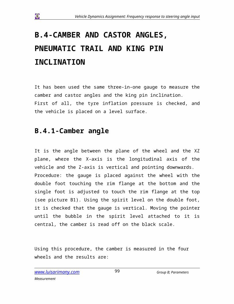
It is the angle between the plane of the wheel and the XZ plane, where the X-axis is the longitudinal axis of the vehicle and the Z-axis is vertical and pointing downwards.Procedure: the gauge is placed against the wheel with the double foot touching the rim flange at the bottom and the single foot is adjusted to touch the rim flange at the top (see picture B1). Using the spirit level on the double foot, it is checked that the gauge is vertical. Moving the pointer until the bubble in the spirit level attached to it is central, the camber is read off on the black scale.

Using this procedure, the camber is measured in the four wheels and the results are:

Front right wheel: -0.5° Front left wheel: -0.5° Rear right wheel: -0.4° Rear left wheel: -0.4°




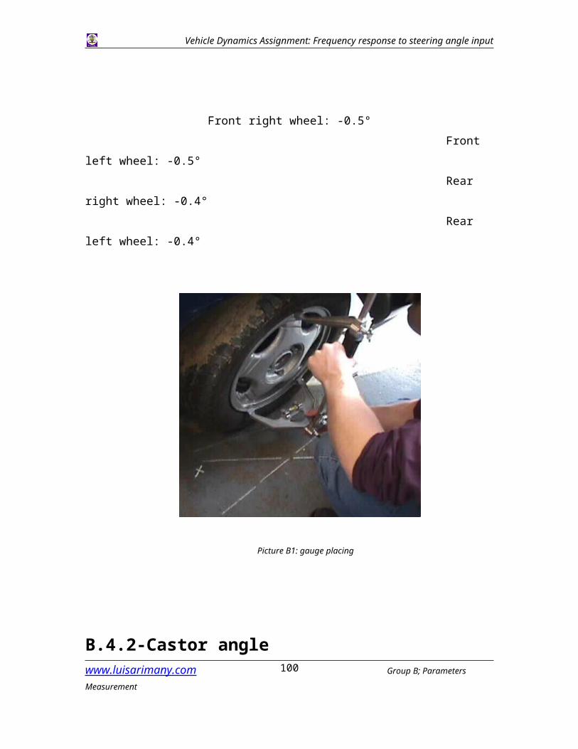
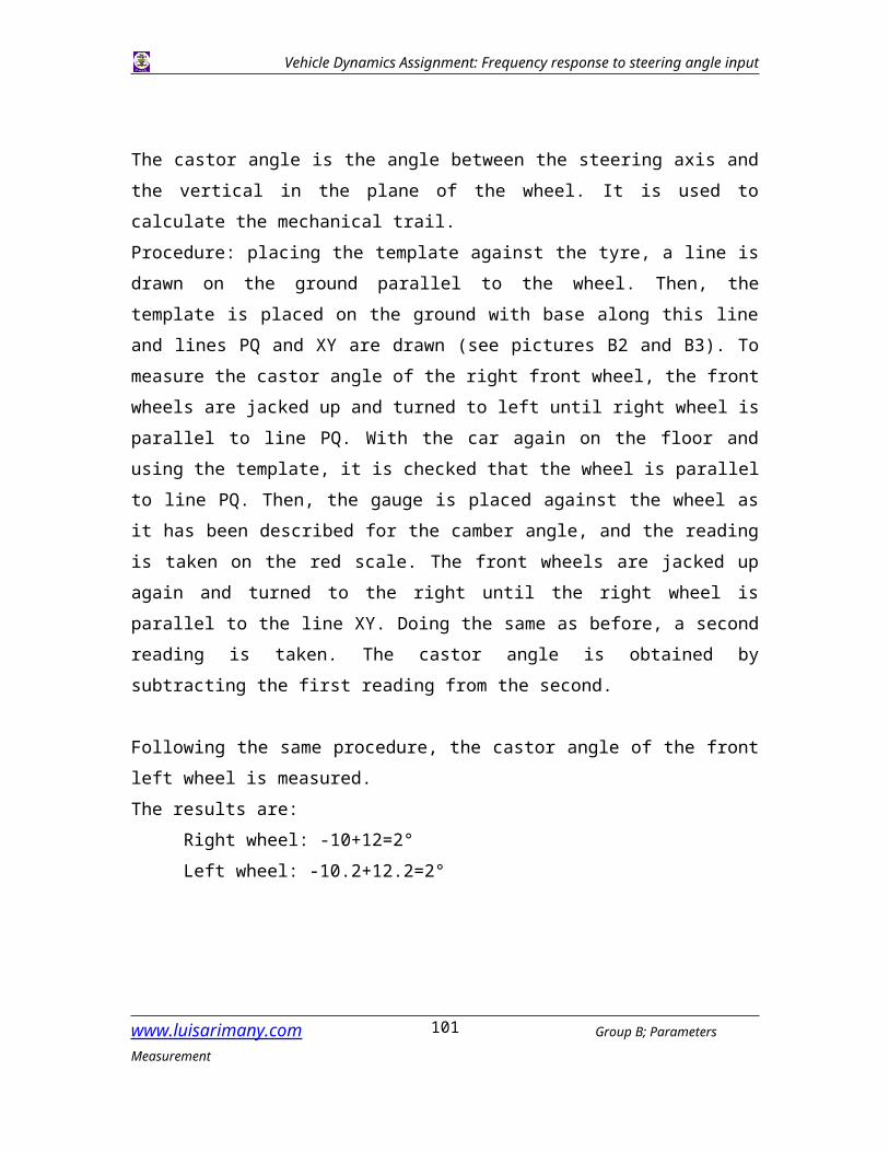
B.4.2-Castor angle

The castor angle is the angle between the steering axis and the vertical in the plane of the wheel. It is used to calculate the mechanical trail.Procedure: placing the template against the tyre, a line is drawn on the ground parallel to the wheel. Then, the template is placed on the ground with base along this line and lines PQ and XY are drawn (see pictures B2 and B3). To measure the castor angle of the right front wheel, the front wheels are jacked up and turned to left until right wheel is parallel to line PQ. With the car again on the floor and using the template, it is checked that the wheel is parallel to line PQ. Then, the gauge is placed against the wheel as it has been described for the camber angle, and the reading is taken on the red scale. The front wheels are jacked up again and turned to the right until the right wheel is parallel to the line XY. Doing the same as before, a second reading is taken. The castor angle is obtained by subtracting the first reading from the second.

Following the same procedure, the castor angle of the front left wheel is measured.


Picture B1: gauge placing



The results are:Right wheel: -10+12=2°Left wheel: -10.2+12.2=2°


Picture B2: placing of the template

Picture B3: reference lines



B.4.3-Pneumatic trail

We couldn’t measure it, so we used data from the manufacturer: 25mm for the unloaded case and 45mm for the laden case.

B.4.4-King pin inclination

The procedure used to measure the king pin inclination is very similar to the one used to measure the castor angle. Using the template as for Castor, mark out the zero, PQ and XY lines on the ground (see pictures B2 andB3). Then jack up the front wheels and turn to the right until the right wheel is parallel to line XY. Lower the car and apply the gauge to the wheel, ensuring that it is approximately vertical by the spirit level on the double foot. Then mark the positions of the feet on the rim (a simple method is to first chalk the rim and then use a black lead pencil or a scriber). Centre the spirit level on the pointer and take the reading on the red scale, this should be approximately 10. With the brakes applied to the front wheels, jack up the axle and turn wheels left until the right wheel is parallel to the line PQ. It is essential that the wheel does not rotate on the axle during this operation. Keeping brakes applied, lower the wheel and apply the gauge to it with the feet coinciding with the marks on the rim. Now move the pointer until the bubble in the spirit level is central and take the reading on the red scale. The king pin inclination is obtained by subtracting the first reading from the second.

Right wheel: -10.5+22=11.5°Left wheel: 9,9+2=11.9°

B.4.5-Discussion

The use of the wheel camber, castor and king pin gauge is not a very accurate method, so we tried to find the values used by the manufacturer. The only value we found was the castor angle, which is 2.11°. The castor angle we had measured was 2°, which is similar, so we can suppose that the values found for the king pin inclination and the camber angle are not very far from the actual ones.




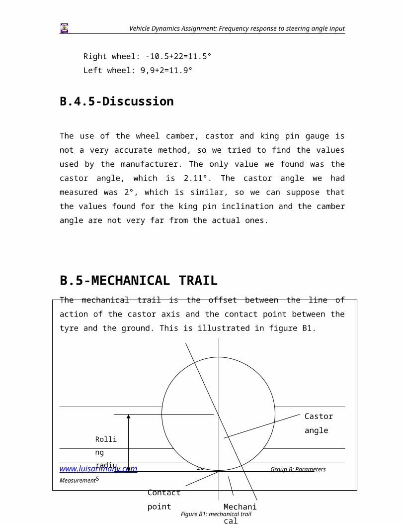
B.5-MECHANICAL TRAILThe mechanical trail is the offset between the line of action of the castor axis and the contact point between the tyre and the ground. This is illustrated in figure B1.

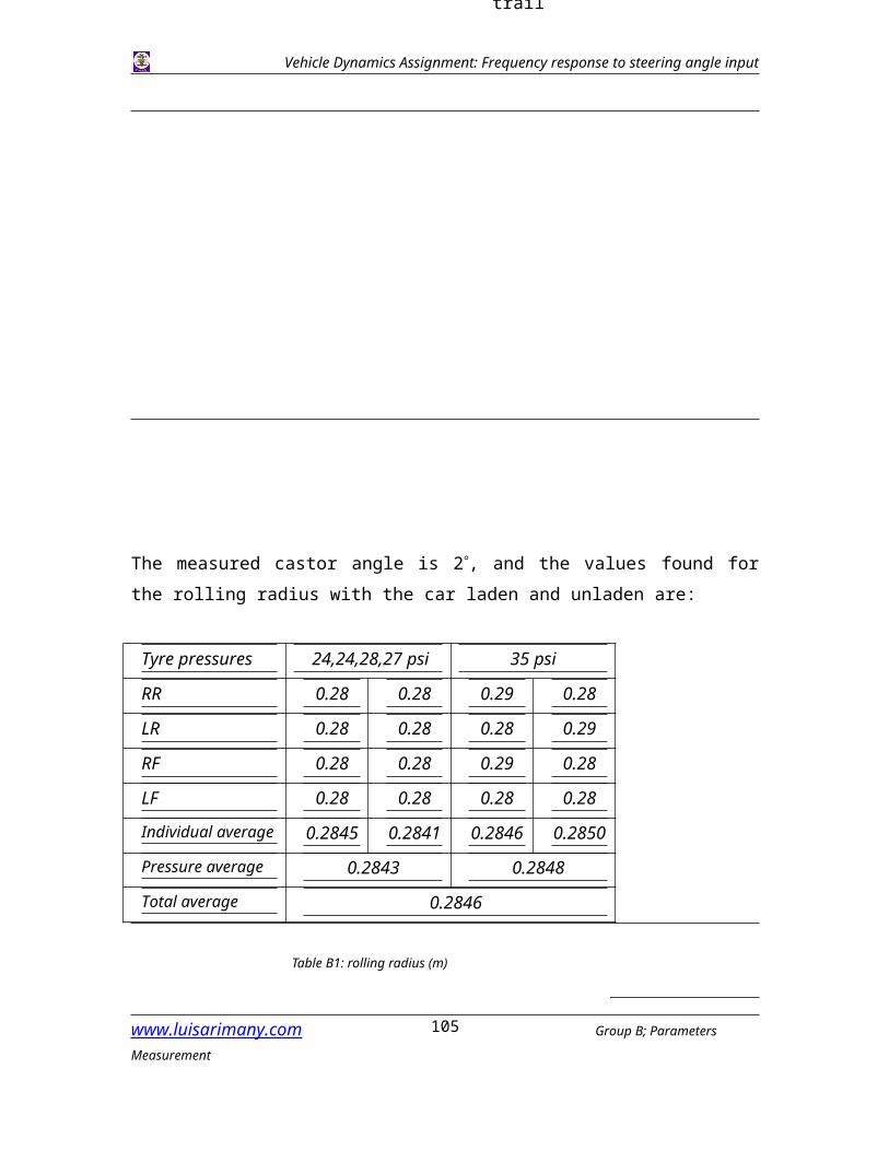
The measured castor angle is 2, and the values found for the rolling radius with the car laden and unladen are:

Tyre pressures 24,24,28,27 psi 35 psi

RR 0.28 0.28 0.29 0.28

LR 0.28 0.28 0.28 0.29

RF 0.28 0.28 0.29 0.28


Rolling radius

Mechanical trail

Contact point

Castor angle

Figure B1: mechanical trail



LF 0.28 0.28 0.28 0.28

Individual average 0.2845 0.2841 0.2846 0.2850

Pressure average 0.2843 0.2848

Total average 0.2846

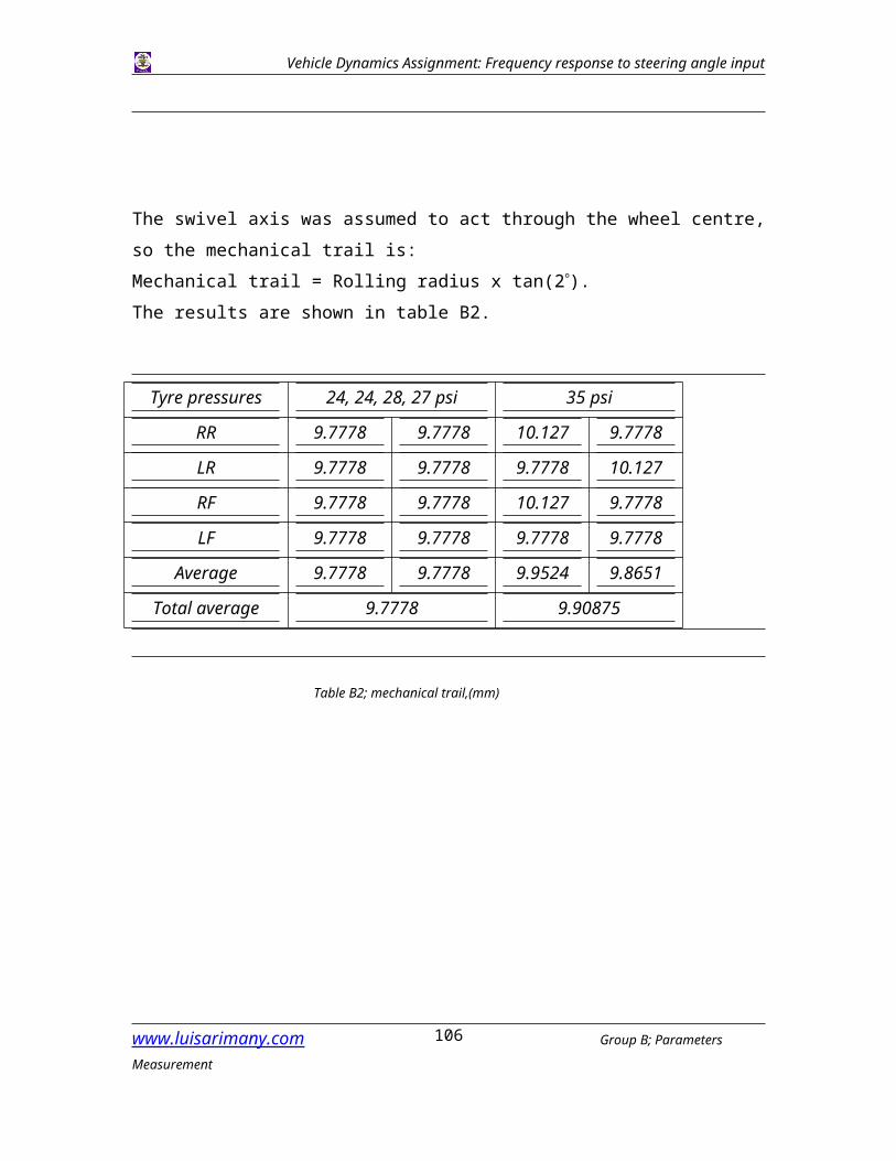
The swivel axis was assumed to act through the wheel centre, so the mechanical trail is:Mechanical trail = Rolling radius x tan(2).The results are shown in table B2.

Tyre pressures 24, 24, 28, 27 psi 35 psi

RR 9.7778 9.7778 10.127 9.7778

LR 9.7778 9.7778 9.7778 10.127

RF 9.7778 9.7778 10.127 9.7778

LF 9.7778 9.7778 9.7778 9.7778

Average 9.7778 9.7778 9.9524 9.8651

Total average 9.7778 9.90875


Table B1: rolling radius (m)

Table B2; mechanical trail,(mm)



B.6-SUSPENSION DERIVATIVES

The aim of this measure is to determine the variation of the camber angle of each wheel within the height of the suspension.

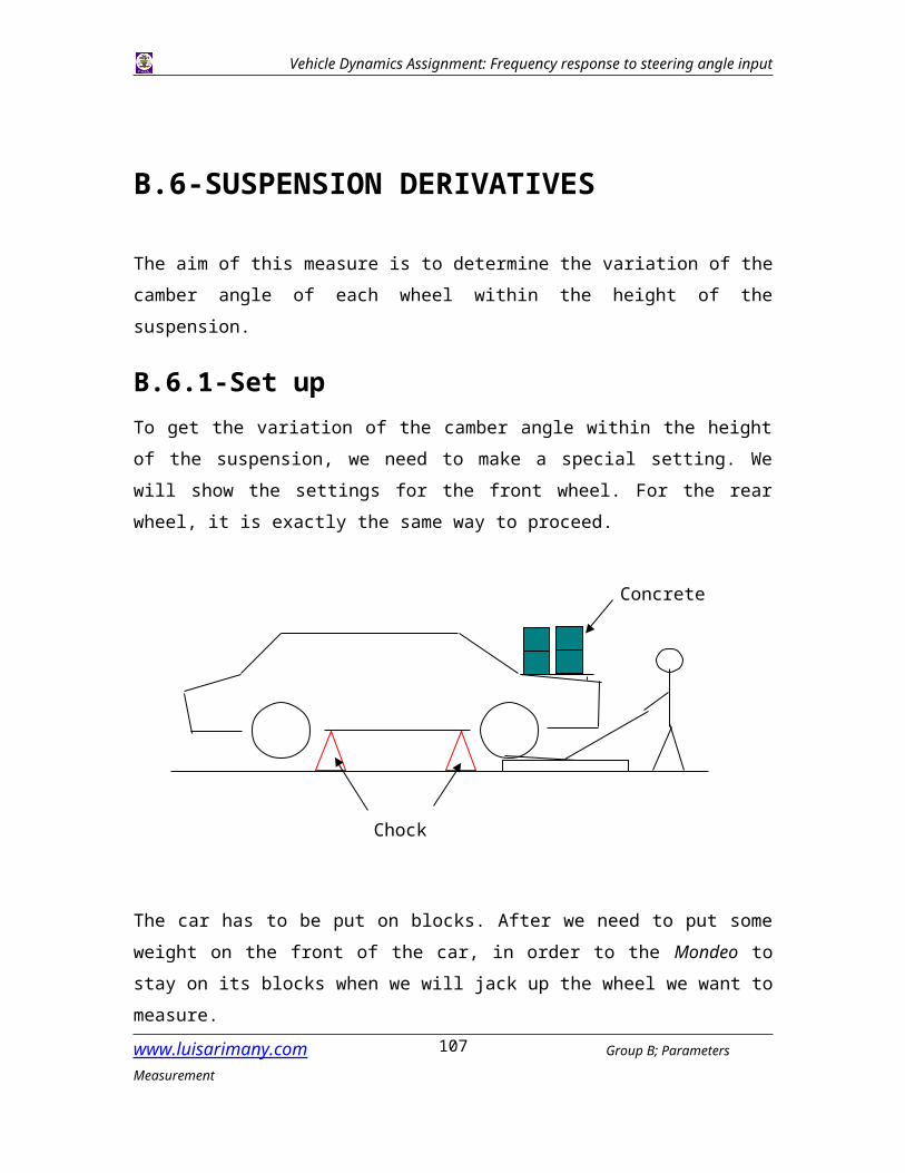
B.6.1-Set up To get the variation of the camber angle within the height of the suspension, we need to make a special setting. We will show the settings for the front wheel. For the rear wheel, it is exactly the same way to proceed.

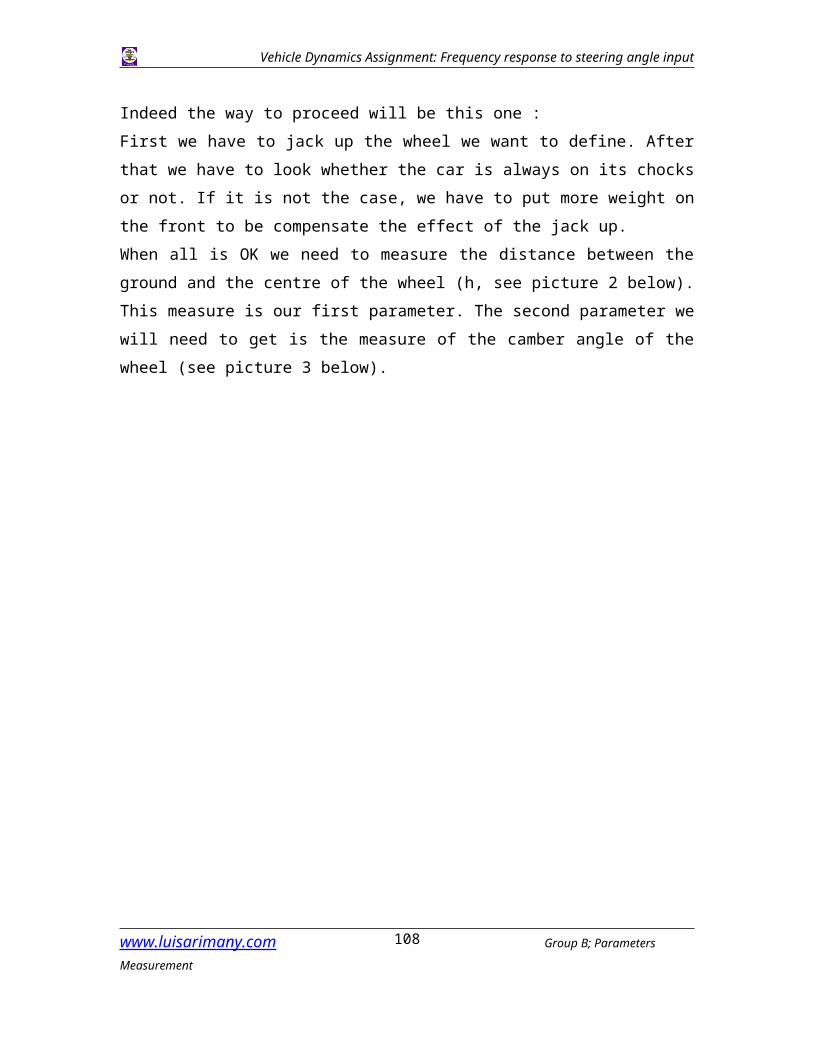
The car has to be put on blocks. After we need to put some weight on the front of the car, in order to the Mondeo to stay on its blocks when we will jack up the wheel we want to measure.Indeed the way to proceed will be this one :First we have to jack up the wheel we want to define. After that we have to look whether the car is always on its chocks or not. If it is not the case, we have to put more weight on the front to be compensate the effect of the jack up.When all is OK we need to measure the distance between the ground and the centre of the wheel (h, see picture 2 below). This measure is our first parameter. The second parameter we will need to get is the measure of the camber angle of the wheel (see picture 3 below).


Concrete Blocks

Chocks



.Thanks to this method, we can get the values of the camber angle for different suspension configuration.

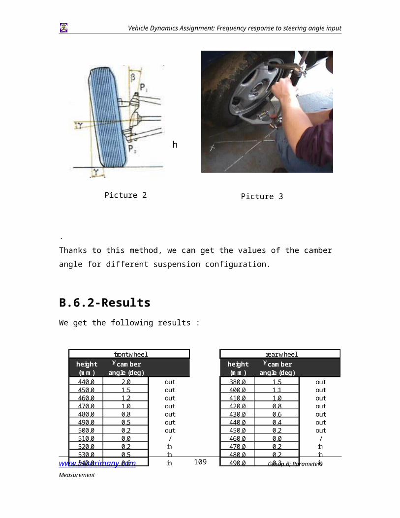
B.6.2-Results We get the following results :


h

Picture 2 Picture 3

height (mm)

camber angle (deg)

440,0 2,0 out450,0 1,5 out460,0 1,2 out470,0 1,0 out480,0 0,8 out490,0 0,5 out500,0 0,2 out510,0 0,0 /520,0 0,2 in530,0 0,5 in540,0 0,6 in

front wheelheight (mm)

camber angle (deg)

380,0 1,5 out400,0 1,1 out410,0 1,0 out420,0 0,8 out430,0 0,6 out440,0 0,4 out450,0 0,2 out460,0 0,0 /470,0 0,2 in480,0 0,2 in490,0 0,3 in

rear wheel




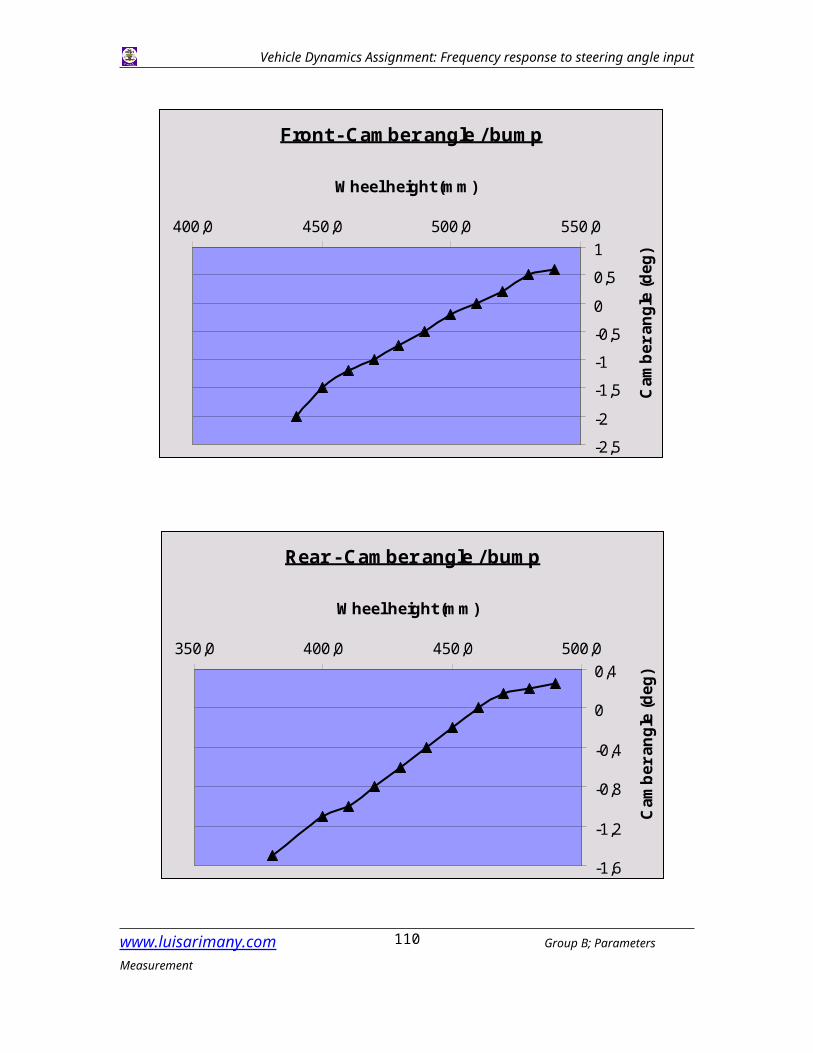
Front - Camber angle / bump

-2,5

-2

-1,5

-1

-0,5

0

0,5

1400,0 450,0 500,0 550,0

Wheel height (mm)

Cam

ber a

ngle

(deg

)

Rear - Camber angle / bump

-1,6

-1,2

-0,8

-0,4

0

0,4350,0 400,0 450,0 500,0

Wheel height (mm)

Cam

ber a

ngle

(deg

)



B.6.3-Conclusion We can see in these two graphs that our results are "quite linear". Indeed the relation between the camber angle and the position of the suspension should be taken as linear, if we take into account the inaccuracy due to the measurement process.




B.7-SUSPENSION DERIVATIVES (II)We will describe the unsuccessful attempt to measure the suspension derivatives. In particular we wanted to measure camber the steering angle and bump steer. We wanted to do that knowing the relevant positions of three points on a plate that was placed on the wheel of the car.

The procedure we attempted is the following:

First it was necessary to place the car on four stands. We were going to start with the front wheels. We had to place the plate we found in the laboratory on the front wheel but we had to find the center of the wheel and also project this on the plate that was placed on the wheel later. We tried to find the center of the wheel with imaginary diameters that were drawn with the help of a tape measure the point of cross-section of the two diameters was the center of the wheel. When we placed the plate on the wheel the surface on the plate was not level, so we could not use a tape measure anymore. We decided to draw arcs with a piece of sting and a pen. We have drawn three arcs the point of intersection of these arcs we called it the center of the plate and the wheel.We then placed a jack underneath the wheel. With the three gauges that were mounted on a tripod and were placed next to the wheel, in theory we could calculate the suspension derivatives we wanted moving the wheel in the bump and rebound condition with the jack. Along with the values from the gauges we needed to measure the distance from the floor to the estimated wheel center (we called this A) and also the distance from the center to the wheel arch (we called this B). We started lifting the wheel and the tripod at intervals of 15mm. We noticed two problems. First that the car was lifted from the stands as we were lifting the jack and also the tripod with the dexion frame that the gauges were mounted on had insufficient stiffness making the measurements unreliable. We took two countermeasures first we added as much weight as possible so when we lifted the jack only the suspension and not the car would move. Secondly we placed a table at the back of the dexion frame to add some support and credibility to our measurements. At last these countermeasures were short lived.




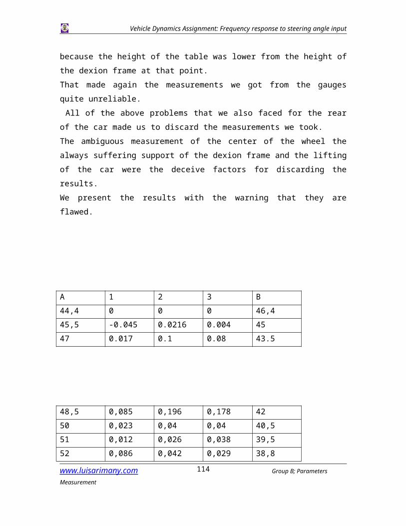
Because after adding all the concrete blocks the car was lifted by the jack. Also after some height the table we used for the dexion frame had to be placed on wooden blocks because the height of the table was lower from the height of the dexion frame at that point. That made again the measurements we got from the gauges quite unreliable. All of the above problems that we also faced for the rear of the car made us to discard the measurements we took. The ambiguous measurement of the center of the wheel the always suffering support of the dexion frame and the lifting of the car were the deceive factors for discarding the results.We present the results with the warning that they are flawed.

A 1 2 3 B44,4 0 0 0 46,445,5 -0.045 0.0216 0.004 4547 0.017 0.1 0.08 43.5

48,5 0,085 0,196 0,178 4250 0,023 0,04 0,04 40,551 0,012 0,026 0,038 39,552 0,086 0,042 0,029 38,8

Picture B1.: gauge measurements for suspension derivatives in the front of the car




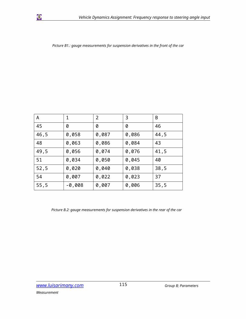
A 1 2 3 B45 0 0 0 4646,5 0,058 0,087 0,086 44,548 0,063 0,086 0,084 4349,5 0,056 0,074 0,076 41,551 0,034 0,050 0,045 4052,5 0,020 0,040 0,038 38,554 0,007 0,022 0,023 3755,5 -0,008 0,007 0,006 35,5

Picture B.2: gauge measurements for suspension derivatives in the rear of the car




B.8-Steering gear ratio

B.8.1-IntroductionThe steering gear ratio (G) gives the relationship between the rotation in the steering

wheel and the correspondent one in the front wheels, so the angle rotated in the steering

wheel is G times the corresponding in the front wheels.

B.8.2-Method

The procedure to measure it is to rotate the steering wheel a certain known angle and

measure the provoked angle variation in the wheel.

The steering wheel rotation will be introduced in steps of 90 degrees, which is an easy

angle to measure just with the help of a tape strip.

This increment will be small enough to give the required accuracy and it doesn’t mean

too many steps from lock to lock.

The angle rotated by the wheel will be measured thanks to dial pads placed under the

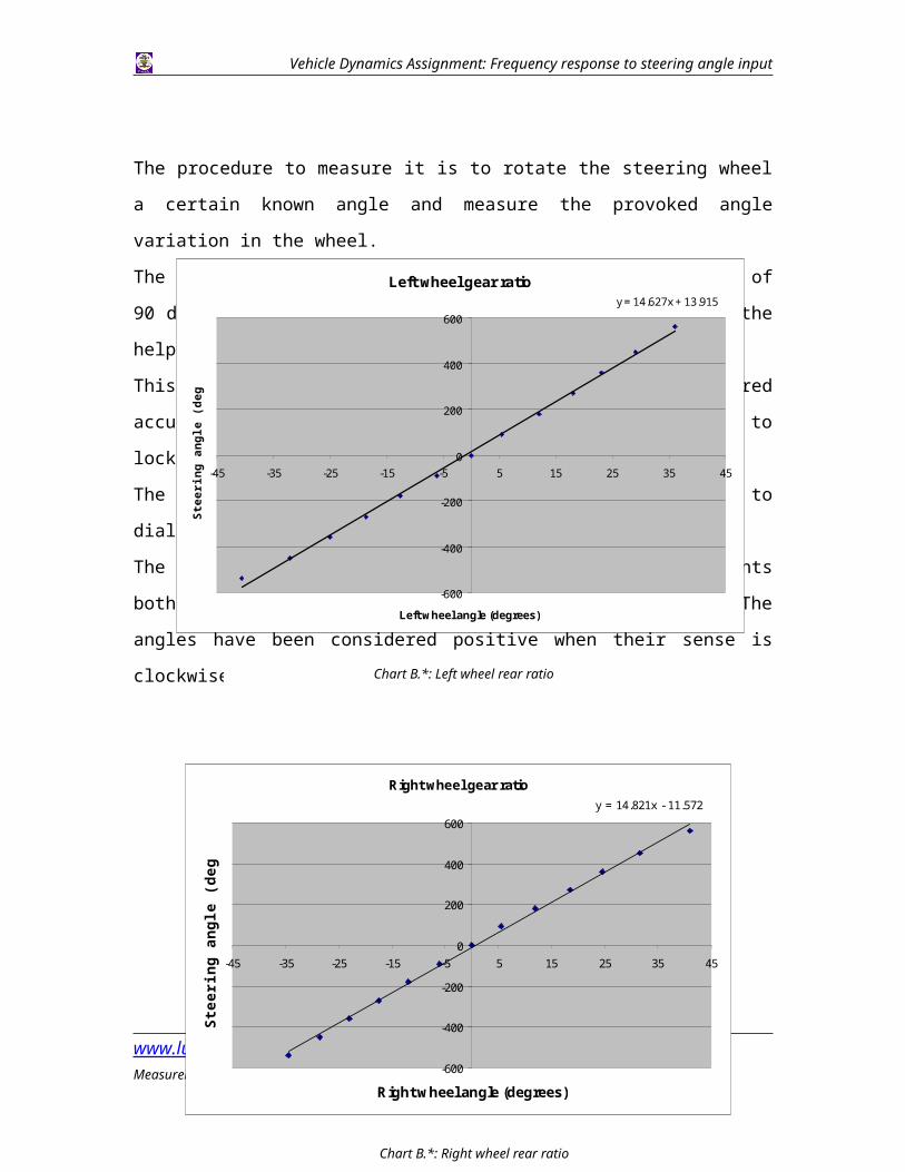
front wheels.

The following graphs give the result of the measurements both for the right front and the

left front wheel. The angles have been considered positive when their sense is clockwise.


Chart B.*: Left wheel rear ratio




Right wheel gear ratioy = 14.821x - 11.572

-600

-400

-200

0

200

400

600

-45 -35 -25 -15 -5 5 15 25 35 45

Right wheel angle (degrees)

Stee

ring

angl

e (d

egre

es)

Chart B.*: Right wheel rear ratio

Left wheel gear ratioy = 14.627x + 13.915

-600

-400

-200

0

200

400

600

-45 -35 -25 -15 -5 5 15 25 35 45

Left wheel angle (degrees)

Stee

ring

angl

e (d

egre

es)

Chart B.*: Left wheel rear ratio



As it was expected, when the steering wheel is rotated to the right (clockwise) the right

wheel is the one that has the biggest angle variation, there is an identical behaviour as far

as the anticlockwise sense and the left wheel is concerned.

Nevertheless it will be considered that there is just one steering gear ratio, independently

the wheel or the sense of rotation.

Then the steering gear ratio will be:

G=(14.821+14.627)/2=14.724




B.9-CORNERING STIFFNESS

Cornering stiffness is defined as the slope of the curve of the cornering force versus the

slip angle.

In a mathematical sense the cornering stiffness is defined as the derivative of the

cornering force with respect to the slip angle at zero slip angle.

Appropriate data were given from the manufacturer of the tyres, in our case Continental.

Relative data can been seen in the next page.

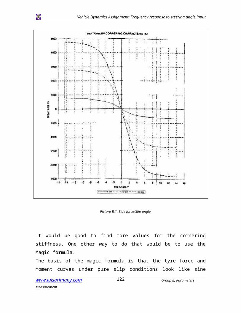
In the figure there are three curves each for a different vertical load.

The first curve corresponds to vertical load of 490N, the second to 2450N, and the third

to 4900N.

From the above and figure B1 we can evaluate the cornering stiffens.

For vertical load of 490N

Cornering stiffness = = =160.7 N/deg


Cornering stiffness = = =693.8 N/deg


Cornering stiffness = = =1000 N/deg

For each case the slope was calculated in the region of zero slip angle at a pressure of 2.1 bar condition that data were gathered.




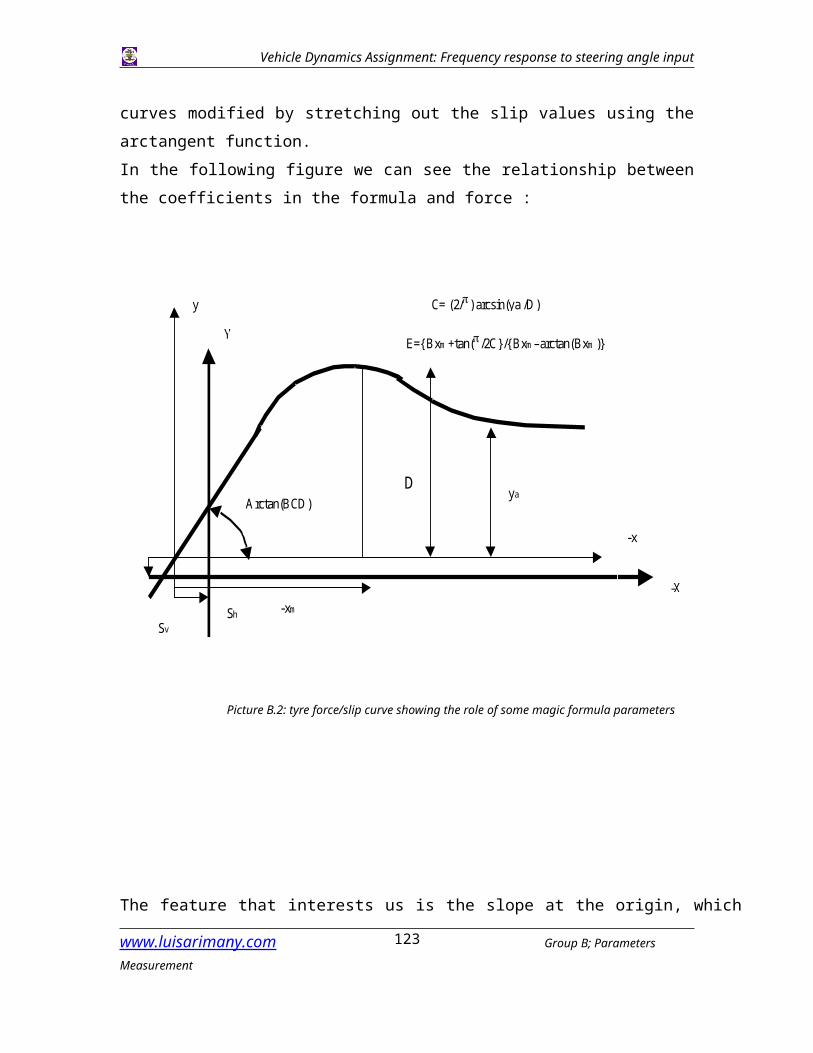
It would be good to find more values for the cornering stiffness. One other way to do that would be to use the Magic formula. The basis of the magic formula is that the tyre force and moment curves under pure slip conditions look like sine curves modified by stretching out the slip values using the arctangent function. In the following figure we can see the relationship between the coefficients in the formula and force :


Picture B.1: Side force/Slip angle



The feature that interests us is the slope at the origin, which is the cornering stiffness. In more detail we can represent BCD as pKy1.sin{2.arctan(FZ/pKy2 )}.(1- pKy3 ||). Subscript “y” represent lateral , FZ is the wheel load, is the camber angle and p’s are parameters. Unfortunately we could not find this additional information so we did not calculate more values. We collocate this method to show that we knew its existence but we were not able to use it.

B.10-FRONT ROLL STIFFNESSwww.luisarimany.com Group B; Parameters Measurement112

-X

-x

yaD

Arctan(BCD)

Y

y

E={Bxm +tan(/2C}/{Bxm –arctan(Bxm )}

C= (2/) arcsin(ya /D)

ShSv

-xm

Picture B.2: tyre force/slip curve showing the role of some magic formula parameters



B.10.1-Introduction

We can define the roll stiffness as the roll moment per unit angle of body roll.

The roll stiffness is certainly a parameter with great influence in the dynamic behaviour

of the vehicle, particularly in the load transfer during cornering therefore it affects the

maximum lateral force available of the tyres.

B.10.2-Method

The method used in this test was strongly determined by the equipment available at the

moment it was performed. Certainly there are more ways to measure the roll stiffness but

it was carried out in the most reliable method with the equipment available.

We focused on the front roll stiffness. The front seats were removed and a moment arm,

which is basically a long beam, was fixed with bolts to the front seats mounting points.

This arm can support load at its two ends, so it can be used to apply a moment to the

vehicle, simulating the situation in a corner.

The total length of the arm is 4090 mm and the distance between the to points were the

load is applied is 3960 mm.

To measure only the front stiffness an axial stand was placed at the rear part of the car,

just at its intersection with the longitudinal axis of symmetry. This way the rear wheels

were not touching the ground, but there was not interference regarding the roll angle

variation.

The torque was applied thanks to 6 weights of 56 lb. (25.2 kg), each of which can be

placed at both of the two ends of the moment arm. The table below represents the

sequence performed changing the position of the weights and therefore applying different

torques to the structure.




The corresponding roll angle was measured thanks to a calibrated inclinometer.

The moment/angle will be considered positive if it is clockwise looking from the driver’s

position.

The graph represents the results obtained, a linear regression was fitted to the data.

B.10.3-Discussion

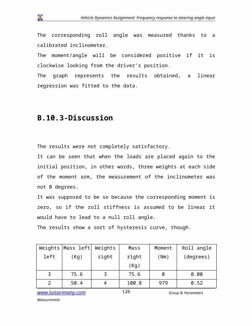
The results were not completely satisfactory.

It can be seen that when the loads are placed again to the initial position, in other words,

three weights at each side of the moment arm, the measurement of the inclinometer was

not 0 degrees.

It was supposed to be so because the corresponding moment is zero, so if the roll stiffness

is assumed to be linear it would have to lead to a null roll angle.

The results show a sort of hysteresis curve, though.

Weights left

Mass left (Kg)

Weights right

Mass right (Kg)

Moment (Nm)

Roll angle (degrees)

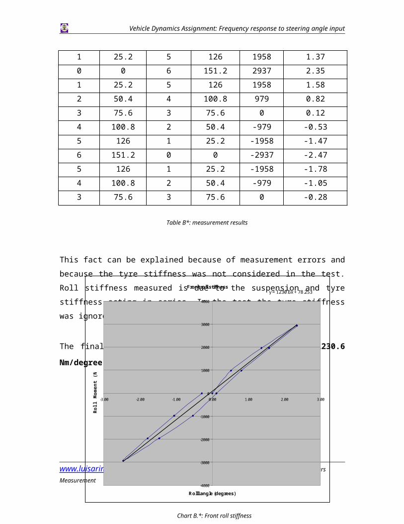
3 75.6 3 75.6 0 0.002 50.4 4 100.8 979 0.521 25.2 5 126 1958 1.370 0 6 151.2 2937 2.351 25.2 5 126 1958 1.582 50.4 4 100.8 979 0.823 75.6 3 75.6 0 0.124 100.8 2 50.4 -979 -0.535 126 1 25.2 -1958 -1.476 151.2 0 0 -2937 -2.475 126 1 25.2 -1958 -1.784 100.8 2 50.4 -979 -1.053 75.6 3 75.6 0 -0.28

www.luisarimany.com Group B; Parameters Measurement114Table B*: measurement results



This fact can be explained because of measurement errors and because the tyre stiffness was not considered in the test. Roll stiffness measured is due to the suspension and tyre stiffness acting in series. In the test the tyre stiffness was ignored.

The final result obtained from the regression was: 1230.6 Nm/degree


Front roll stiffnessy = 1230.6x + 78.253

-4000

-3000

-2000

-1000

0

1000

2000

3000

4000

-3.00 -2.00 -1.00 0.00 1.00 2.00 3.00

Rolll angle (degrees)

Rol

l Mom

ent (

Nm

)

Chart B.*: Front roll stiffness



B.11-SUSPENSION DAMPING FACTOR

B.11.1-Requirement to perform the test

an accelerometer a data capture module a low pass filter card a laptop computer for acquisition a software (to treat the signal : voltage variation converted into acceleration or

displacement)

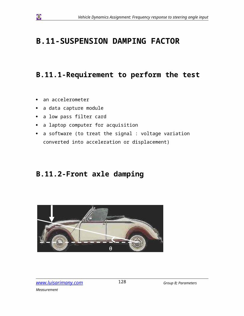
B.11.2-Front axle damping

An accelerometer allows us to determine the displacement (from acceleration) when we apply an prompted load at the front. The application point of the load corresponds to the position of the accelerometer. The load is applied manually on the bonnet in order to have a vertical force as seen in the picture. The accelerometer is connected to a data capture module. Then, to treat the signal, the voltage is converted into a acceleration value.




Basically, we need intrinsically the displacement. Indeed, we are going to use the logarithmic decrement method and the ratio of the 2 first peaks in displacement allows us to deduce the damping ratio.

As the logarithmic decrement is d = ln (d1 / d2)

Undamped natural freq. = wN = d / z.Td

Damping ratio z = d / (42 + d2)

Phasing problems

5 measurements are performed. The issue here is that the responses are not in phase with each other. Indeed, the manually applied load does not allow a trigger at a fixed time.Before starting to average the responses and integrate them, the aim is to correct the phasing between the 5 curves. The first one is chosen as the reference and the other ones are phased from the maximal value of their first peak :





Front axle responses (k.g)-(ms)

0,00E+00

5,00E-01

1,00E+00

1,50E+00

2,00E+00

2,50E+00

3,00E+00

242 units phasing

45 units phasing

48 units phasing

89 units phasing

accelerations : arbitrary units k.gtotal sample time : 2s, unit msgraduation = 50ms

Front axle response (corrected phasing)

0,00E+00

5,00E-01

1,00E+00

1,50E+00

2,00E+00

2,50E+00

3,00E+00



Correction – Average

Then, the average value of the acceleration is calculated.

Note : We are just interested in the ratio of the amplitudes between the first and the second peak of the displacement curve.

Basically, the accelerometer gives us –1.90V for –1g acceleration, 0V for 0g acceleration

and +1.85V for 1g acceleration.

It is a servo accelerometer, calibrated to be quasi linear. But it is not used to lose time to

convert the data in order to have the values of acceleration. Put that the units for

acceleration, then for velocity and finally for displacements are given in K1 x g, K2 x m/s

and K3 x m (where Ki are factors that will not be reckoned).

Thus an average curve is calculated with Excel.

It will be our reference curve that will be integrated twice in order to determine the

displacement of the front of the car.


Servo-accelerometer calibration

-3

-2

-1

0

1

2

3

-1,5 -1 -0,5 0 0,5 1 1,5

Vertical acceleration (g)

Resp

onse

vol

tage

(V)



Note : On the previous curve, we can check that the gravitational acceleration (g) corresponding to a 1.90V response is the acceleration measured just before and after the perturbation. That is the case !


acceleration : arbitrary units k.gacquisition time : 5s



Integration – Velocity - Displacement

The acceleration is something like A.e-wt cos ( wt + f ). It needs to be integrated a first time to find the velocity curve. Integration is performed with Excel :

The curve is not too bad and allows us to integrate it a second time :


Velocity (first interation)

-3,00E+01

-2,00E+01

-1,00E+01

0,00E+00

1,00E+01

2,00E+01

3,00E+01

4,00E+01

velocity : arbitrary units k.m/stotal sample time : 3s

Displacement (second integration)

-3,50E+03

-3,00E+03

-2,50E+03

-2,00E+03

-1,50E+03

-1,00E+03

-5,00E+02

0,00E+00

5,00E+02

1,00E+03

displacement : arbitrary units k.mtotal sample time : 3s



Logarithmic decrement

d1 / d2 = 3060 / 271 = 11.3 thus d = ln (d1 / d2 ) = 2.42Td = 430 ms = 0.43 sDamping ratio z = d / (42 + d2) = 2.42 / (39.47 + 5.85)1/2 = 0.35As undamped natural freq. = wN = d / z.Td = 2.42 / (0.35 x 0.43) = 15.5 rad/s

wN = 15.5 rad/s z = 0.35

The critical damping coefficient can be calculated as following : Cc = 2m.wN with m the vehicle sprung mass acting at the front (in this case mtot = 1280 kg = total vehicle mass + acquisitions operator mass – sprung mass). The ratio between the front weight repartition and the rear one is about 3 for 2 thus the front axle sprung mass is about 770 kg.

Vertical Damping Coefficient Cv = z.Cc = 2m.d/Td = 8550 Ns/m

Cfront = 8550 Ns/m

Assuming Cwheel is quite the same for each wheel, we deduce the damping coefficient relative to a single wheel.The front dampers are in // hence : Cfront = Cfl + Cfr


-3,50E+03

-3,00E+03

-2,50E+03

-2,00E+03

-1,50E+03

-1,00E+03

-5,00E+02

0,00E+00

5,00E+02

1,00E+03

d1

d2

Td



Indeed, at equilibrium F = Cf.x = Cfr.x + Cfl.x = (Cfl + Cfr ).xIt means that Cwheel = 4250 Ns/mIn the real world, while we push the front vertically, the rear does not only spin around its transversal axle : it also moves down a bit.

That means that Cfront is a kind of damping coefficient for the whole vehicle “weighted for the front” instead of the intrinsic front damping coefficient. Hence, we can assume that the intrinsic Ci-front is smaller.If 1/10th of the front displacement occurs also at the rear, from the equilibrium in resultants, the equation becomes something like : x.C = x.Ci-front + 0,1x.Ci-rear


x xF F

CflCfr Cf

L

Rear also moves

x x/10



Hence C = Ci-front + 0,1.Ci-rear = 2.Cwheel + 0,2.Cwheel = 2,2.Cwheel

Assuming that Cfl = Cfr = Crr = Crl = Cwheel,Cwheel = 3'880 Ns/m

This result is quite good. Indeed the theory finds something like 2'000 Ns/m per wheel. The initiated displacement at the rear could also be larger. The effect would be to reduce again C per wheel.

Last year’s test was not as disappointing as they pretended. The problem was that they made a mistake in their assumptions. Of course the dampers are mounted in parallel but in this case the formula is not 1/Ctot = 1/C// + 1/C// etc…It is obvious that this formula corresponds to series mounting. Indeed, if 2 springs are mounted in series, the first one with K quasi infinite and the other one with K = 1N/m, the global spring equivalent to this mounting will have its K about 1 N/m. Stiffness of springs in series is always determined by the weakest stiffness of the chain ! Then, they pretended that the dampers were in parallel and they used the formula for series mountings !

The influence of the tyre inner damping coefficient is very hard to estimate. It could be interesting to perform the same test only onto rims.

Using friction plates in order to allow the lateral movement of the wheels could also be valuable.

Finally we can imagine a test where the rear suspensions are disconnected during the test of the front one (and vice versa to avoid to affect measures by the reaction of one suspension track onto the other)




B.11.3-Rear axle Damping

The same method is followed but the graphs are not so exploitable.


0,00E+00

5,00E-01

1,00E+00

1,50E+00

2,00E+00

2,50E+00

3,00E+00

3,50E+00

4,00E+00

4,50E+00

Série1Série2Série3Série4Série5

237 units phasing

66 units phasing

184 units phasing

198 units phasing

acc. : arbitrary units k.gtotal sample time : 2s, unit ms,graduation = 50ms

acceleration (phasing corrected)

0,00E+00

5,00E-01

1,00E+00

1,50E+00

2,00E+00

2,50E+00

3,00E+00

3,50E+00

4,00E+00

4,50E+00

Série1Série2Série3Série4Série5




average acceleration (rear axle)

0,00E+00

5,00E-01

1,00E+00

1,50E+00

2,00E+00

2,50E+00

3,00E+00

3,50E+00

4,00E+00

4,50E+00

acceleration : arbitrary units k.gtotal sample time : 3s… trends curve

Velocity (first integration)

-8,00E+01

-6,00E+01

-4,00E+01

-2,00E+01

0,00E+00

2,00E+01

4,00E+01

6,00E+01

8,00E+01

velocity : arbitrary units k.m/stotal sample time : 3s



We can notice on the previous graph that there is no real second peak in order to calculate the logarithmic decrement. Anyway, the log decrement method reaches here its limits. Indeed the response is quasi non oscillatory. The perturbation is well represented but after that the rear moves higher than its equilibrium position and slowly moves down to its starting position.

The fact that it is almost impossible to apply a strictly vertical force onto the rear can explain the results. Indeed, when applying the load onto the rear, the car also tends to move forward. The force is then a non purely vertical one that acts as well onto the front suspension and that also depends on the longitudinal damping characteristics of the vehicle.






Documents

Rolling Radius - Luis Arimany | La Web de Luis Arimany€¦ · Web view · 2015-05-25B.1.1-Description of the experiment. The inertia of the wheel about its spin axis is determined