Role of Models in Population Biology

Understanding Predicting Implications for

empirical work

0

50

100

150

0 10 20 30 40 50

Days

Den

sity

Rotifers(after Halbach 1979)

0

50

100

150

0 10 20 30 40 50Days

Den

sity

15 oC

25 oC

Pheasants

Data collection Regional and statewide abundance

estimates Predicting quality of coming

pheasant season

2003: 1.36 pheasants per 100 miles2004: 1.75 pheasants per 100 miles 29% increase

Commission's upland game program manager, Scott Taylor

Nebraska's pheasant population is at its highest level since 1995, according to rural mail carrier surveys conducted in the spring and summer by the Nebraska Game and Parks Commission.

The surveys indicate the population is improved over last year and substantially improved over the previous five-year average.

Time Series

0

5

10

15

20

1940 1960 1980 2000 2020

Time [years]

Ph

easa

nts

/ 1

00 m

iles

0.0

2.0

4.0

6.0

8.0

10.0

12.0

14.0

16.0

18.0

20.0

1940 1950 1960 1970 1980 1990 2000 2010

Time [years]

Ph

easa

nts

/ 1

00 m

iles

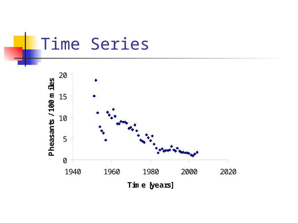
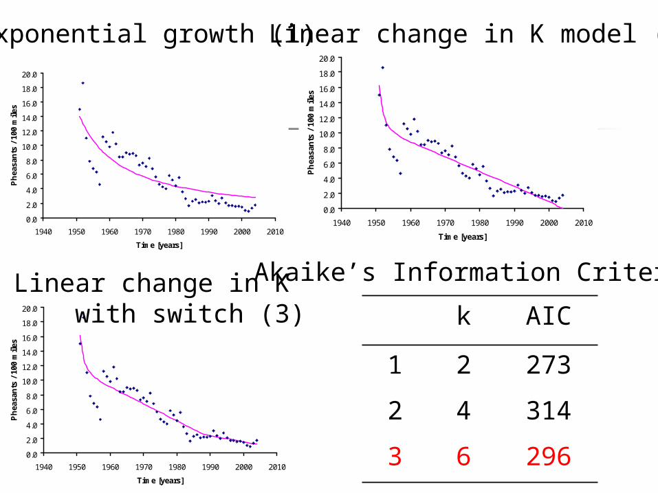
Exponential growth (1)

0.0

2.0

4.0

6.0

8.0

10.0

12.0

14.0

16.0

18.0

20.0

1940 1950 1960 1970 1980 1990 2000 2010

Time [years]

Ph

easa

nts

/ 1

00 m

iles

Linear change in K model (2)

0.0

2.0

4.0

6.0

8.0

10.0

12.0

14.0

16.0

18.0

20.0

1940 1950 1960 1970 1980 1990 2000 2010

Time [years]

Ph

easa

nts

/ 1

00 m

iles

Linear change in K with switch (3)

tK

Nr

ttt

t

eNN

1

1

bd

ca

dc

bat

KK

KKs

sttKK

sttKKK

,

,

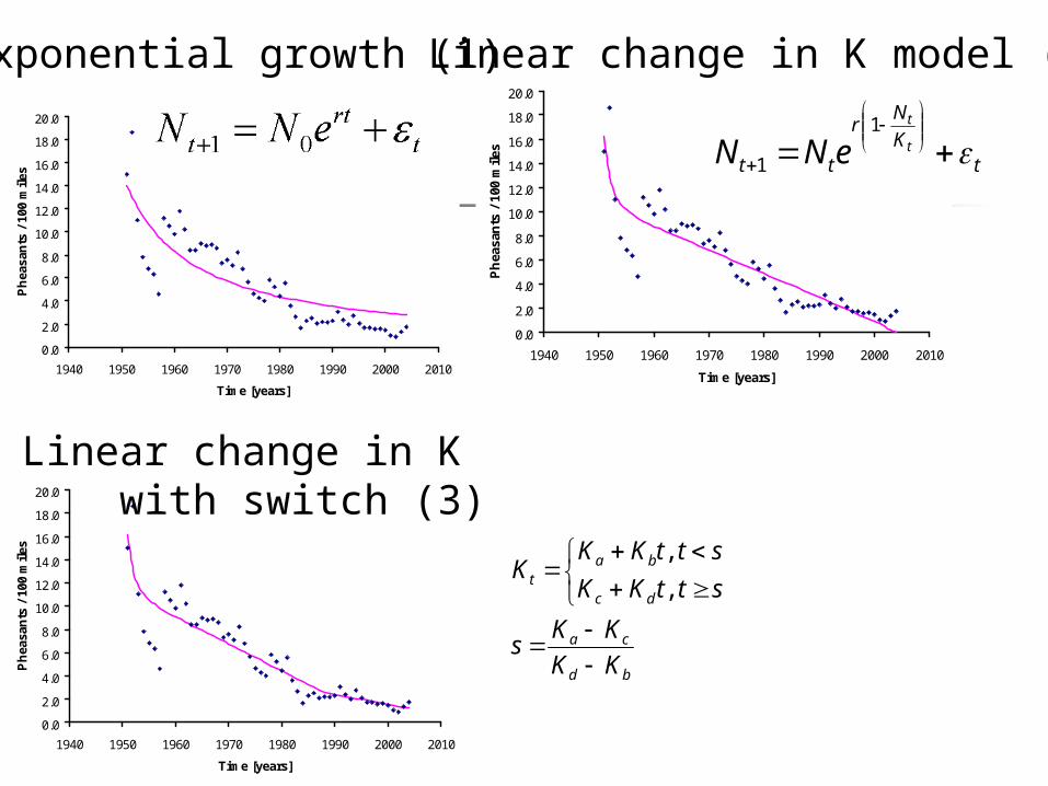
Akaike’s Information Criterion

AIC = -2L + 2k L = log likelihood ~ probability the

model is correct, given the data k = number of parameters in the

model Low AIC is better

0.0

2.0

4.0

6.0

8.0

10.0

12.0

14.0

16.0

18.0

20.0

1940 1950 1960 1970 1980 1990 2000 2010

Time [years]

Ph

easa

nts

/ 1

00 m

iles

Exponential growth (1)

0.0

2.0

4.0

6.0

8.0

10.0

12.0

14.0

16.0

18.0

20.0

1940 1950 1960 1970 1980 1990 2000 2010

Time [years]

Ph

easa

nts

/ 1

00 m

iles

Linear change in K model (2)

0.0

2.0

4.0

6.0

8.0

10.0

12.0

14.0

16.0

18.0

20.0

1940 1950 1960 1970 1980 1990 2000 2010

Time [years]

Ph

easa

nts

/ 1

00 m

iles

Linear change in K with switch (3)

Akaike’s Information Criterion

k AIC

1 2 273

2 4 314

3 6 296

A simple (discrete) population model

Nt+1 = Nt + B - D + I – Epop next time period

pop. this time period

births deaths immigrants emigrants

Change in abundance

Nt+1 - Nt = B - D + I - E

N = B - D + I - E

Basic closed population model

Simplifying assumption: no movement between populations Abundance

Nt+1 = Nt + B – D

Change in abundance

N = B – D

if B > D then population increaseif B< D then population decreaseif B = D then stable population

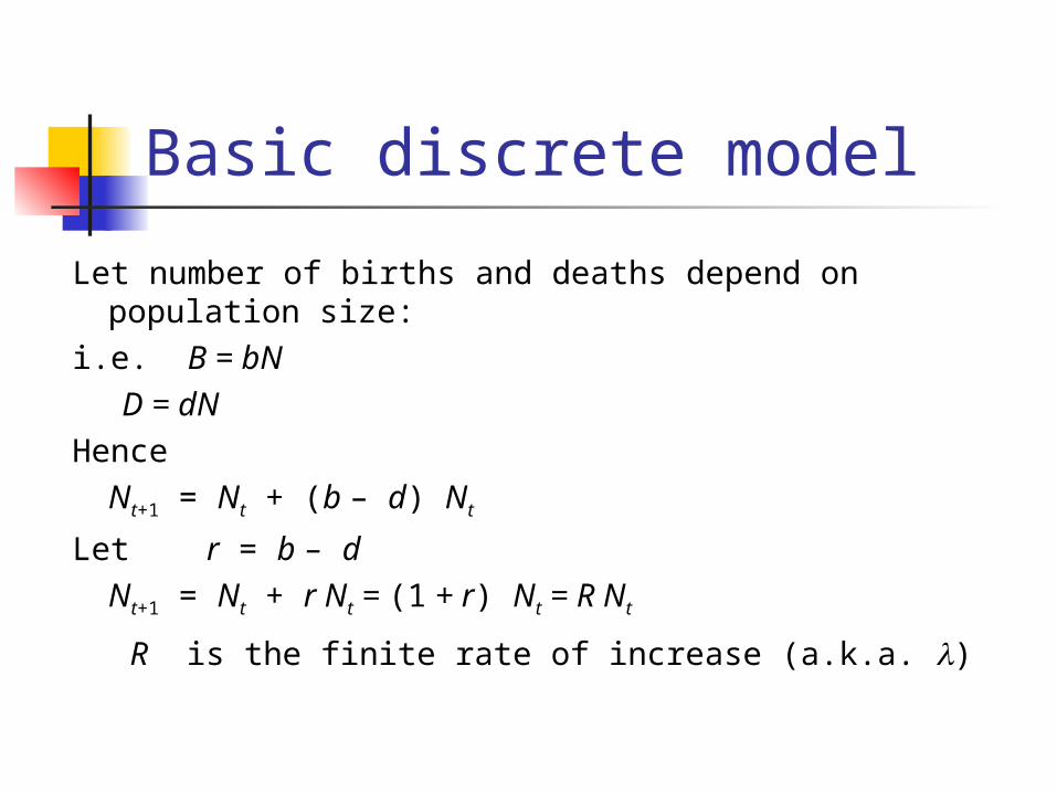
Basic discrete model

Let number of births and deaths depend on population size:

i.e. B = bN D = dNHence

Nt+1 = Nt + (b – d) Nt

Let r = b – dNt+1 = Nt + r Nt = (1 + r) Nt = R Nt

R is the finite rate of increase (a.k.a. )

Varying

0500

1000

15002000250030003500

0 1 2 3 4 5 6 7 8 9 10

time (t)

po

pu

lati

on

siz

e N

(t)

1.0

1.2

0.8

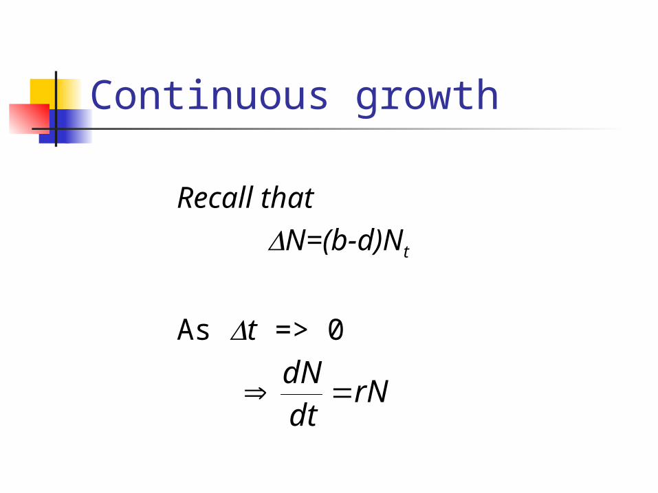
Continuous growth

Recall that

N=(b-d)Nt

As t => 0

rNdt

dN

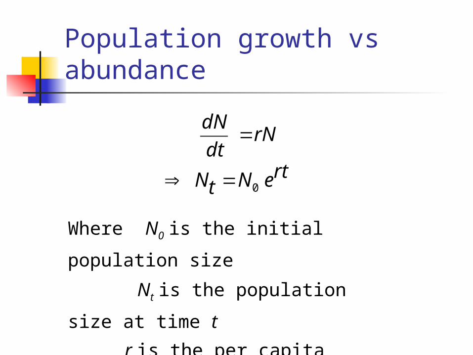
Population growth vs abundance

rteNtN

rNdt

dN

0

Where N0 is the initial population size

Nt is the population size at time t

r is the per capita growth rate

Different Names for r

Instantaneous rate of increase Intrinsic rate of increase Malthusian parameter Per capita rate of population

increase over short time interval

r = b – d

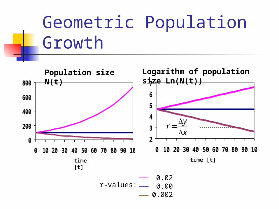
Geometric Population Growth

time [t]

Population size N(t)

0.020.00

-0.002

r-values:

time [t]

Logarithm of population size Ln(N(t))

yr

x

Discrete vs continuous growth

Discrete vs continuous growth

Discrete growth across a time interval; birth and death discrete

realistic; hard to generalize results

Continuous instantaneous

growth;

birth and death continuous process

abstraction; easier to generalize

results

Ln() = r

= er

r > 0 > 1r = 0 = 1r < 0 0 < < 1

Model Assumptions

Model Assumptions Closed population Constant b and d Population grows exponentially indefinitely No genetic structure No age or size structure Species exist as single panmictic population

unstructured (random-mating) populations

Pheasants of Protection Island(Data from Lack 1967)

1

10

100

1,000

10,000

1937 1938 1939 1940 1941 1942 1943Year

Po

pu

lati

on

siz

e (

N)

1937 8 birds1938 30 birds

R = 30/8 = 3.75r = ln(3.75) = 1.3217

0

2,000

4,000

6,000

8,000

10,000

12,000

1937 1938 1939 1940 1941 1942 1943Year

Po

pu

lati

on

siz

e (

N)

Density dependence Population growth is affected

by limited resources food breeding sites territories

Density dependent factors influence birth and death rates b and d are not constant

Logistic population growth

Population size (N)

Population size (N)

b

b

Allee effect

Effects of crowding: decreased reproduction

Effect of density on fecundity in the Great Tit Parus major (Lack 1966)

Density dependence in song sparrows (after Arcese and Smith 1988, Smith et al.

1991)

0123456

0 20 40 60 80

Number of beeding females

Surviving young per female

0

0.1

0.2

0.3

0 20 40 60 80 100

Number of territorial males

Proportion of floaters among males

00.10.20.30.40.50.6

20 40 60 80 100 120 140 160

No adults in autumn

Proportion of surviving juveniles

Density Dependence in Death Rate

Increased crowding increased death rate

d = d0 + c N

d0 : death rate under uncrowded conditions

c : measures strength of density dependence

N : current population size

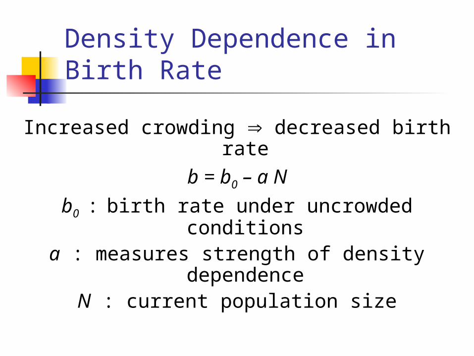
Density Dependence in Birth Rate

Increased crowding decreased birth rate

b = b0 – a N

b0 : birth rate under uncrowded conditions

a : measures strength of density dependence

N : current population size

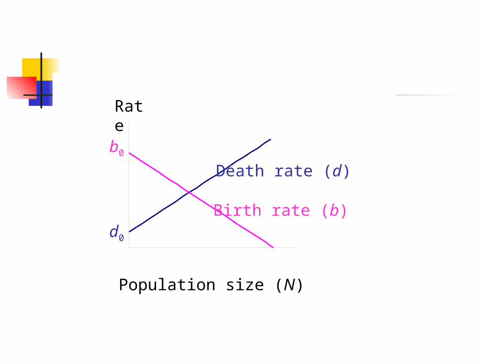
Population size (N)

Rate

b0

d0

Death rate (d)

Birth rate (b)

Interpretation of Carrying Capacity K Defined as the level of abundance above

which the population tends to decline It is population specific: depends on

available resources and space (quality and quantity), abundance of predators and competitors

It is an abstraction: crude summary of interactions of a population with environment

Units are in number of individuals supported by environment

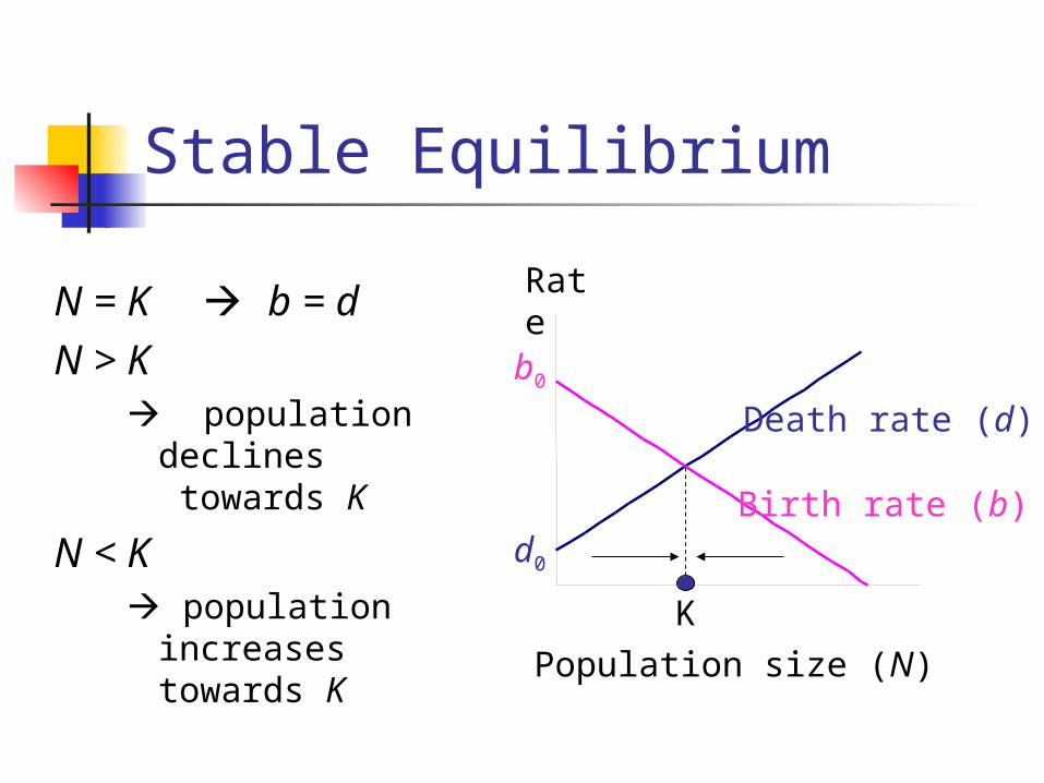
Stable Equilibrium

N = K b = dN > K

population declines towards K

N < K population

increasestowards K

Population size (N)

Rate

b0

d0

K

Death rate (d)

Birth rate (b)

Carrying capacity, K

1dN N

rNdt K

Unused proportion of carrying capacity

14% of area is white or “unused”

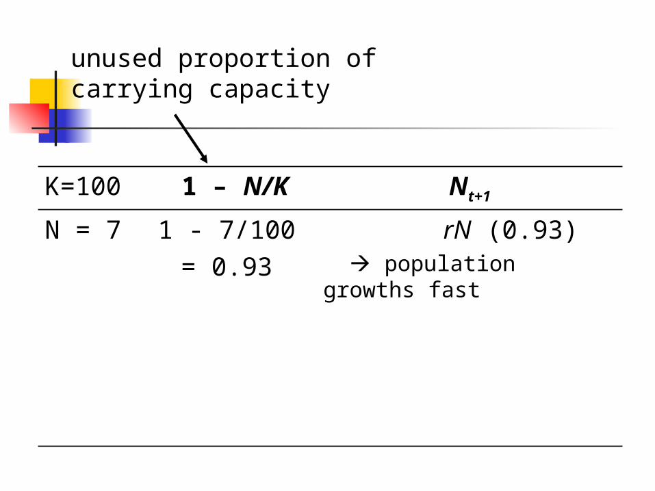
K=100

1 – N/K Nt+1

N = 7 1 - 7/100= 0.93

rN (0.93) population growths fast

unused proportion of carrying capacity

K=100

1 – N/K Nt+1

N = 7 1 - 7/100= 0.93

rN (0.93) population growths fast

N = 98

1 - 98/100= 0.02

rN (0.02) population growths slowly

unused proportion of carrying capacity

K=100

1 – Nt/K Nt+1

N = 7 1 - 7/100= 0.93

rN (0.93) population growths fast

N = 98

1 - 98/100= 0.02

rN (0.02) population growths slowly

N = 105

1 - 105/100= -0.05

rN (-0.05) population declines

unused proportion of carrying capacity

Logistic Growth Curve

0

20

40

60

80

100

120

140

160

180

200

0 20 40 60 80 100

Time (t)

Popu

latio

n si

ze (N

)

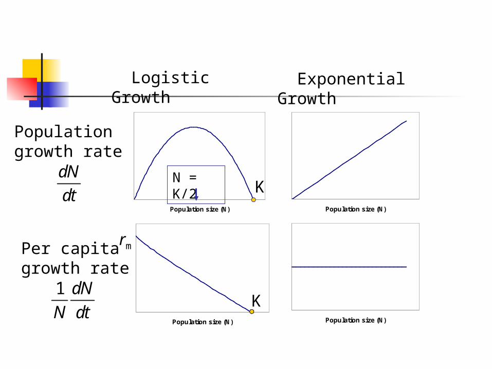
Population size (N)

Population growth rate

Logistic Growth

KdN

dtN = K/2

Population size (N)

Exponential Growth

Population size (N)

Per capita growth rate

K1 dN

N dt

rm

Population size (N)

Time Lag (t) Sometimes individuals do not

immediately adjust their growth and reproduction when resources change, and these delays can affect population dynamics

Causes Seasonal availability of resources Growth responses of prey populations Age and size structure of consumer

populations

1 tdN N

rNdt K

Time Lag Delay differential equation Important parameters:

Length of time lag, “Response time” = 1/r

r controls population growths 0 < r < 0.368

population increases smoothly to K 0.368 < r < 1.570

damped oscillations r > 1.570

stable limit cycle

Time (t)

Po

pu

lati

on

siz

e (

N)

“medium” r damped oscillations

Time (t)

Po

pu

lati

on

siz

e (

N)

“small” r

Time (t)

Po

pu

lati

on

siz

e (

N)

Period ( 4

Amplitude(increases with r)

“large” r stable limit cycle

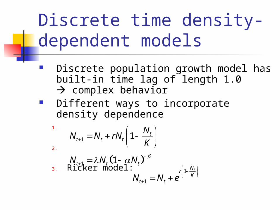
Discrete time density-dependent models Discrete population growth model has

built-in time lag of length 1.0 complex behavior

Different ways to incorporate density dependence

1.

2.

3. Ricker model:

1 1 tt t t

NN N rN

K

1

1

tNr

Kt tN N e

1 1t t tN N N

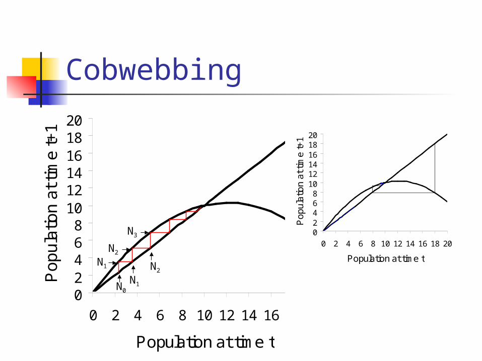
Cobwebbing

02468

101214161820

0 2 4 6 8 10 12 14 16 18 20

Population at time t

Po

pu

latio

n a

t tim

e t+

1

02468

101214161820

0 2 4 6 8 10 12 14 16 18 20

Population at time t

Po

pu

latio

n a

t tim

e t+

1N0

N1

N1 N2

N2

N3

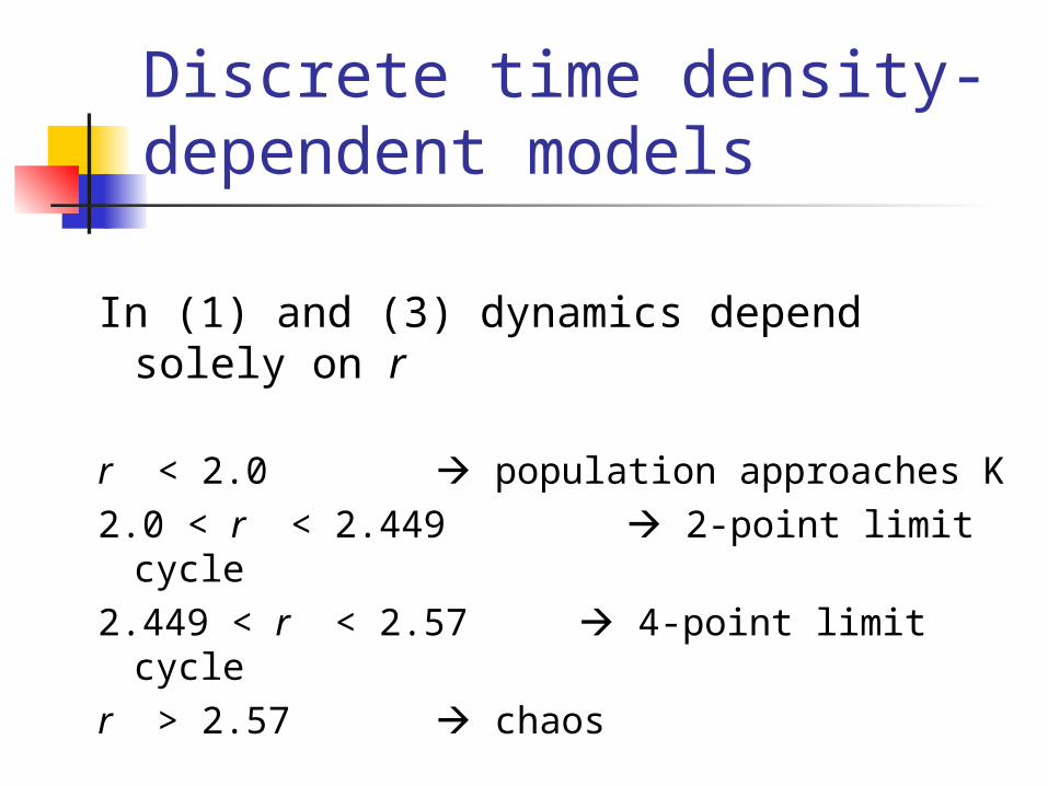
Discrete time density-dependent models

In (1) and (3) dynamics depend solely on r

r < 2.0 population approaches K

2.0 < r < 2.449 2-point limit cycle2.449 < r < 2.57 4-point limit cycler > 2.57 chaos

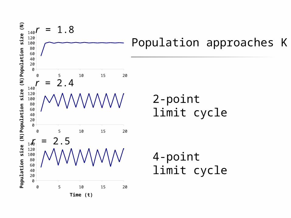
020406080

100120140

0 5 10 15 20

Po

pu

lati

on

siz

e (

N) r = 1.8

Population approaches K

020406080

100120140

0 5 10 15 20

r = 2.4

Po

pu

lati

on

siz

e (

N)

2-point limit cycle

020406080

100120140

0 5 10 15 20

Time (t)

r = 2.5

Po

pu

lati

on

siz

e (

N)

4-point limit cycle

r=1.8

N(t)

N(t

+1)

0.0 0.2 0.4 0.6 0.8 1.0

0.0

0.2

0.4

0.6

0.8

1.0

N(t)

N(t

+1)

N0

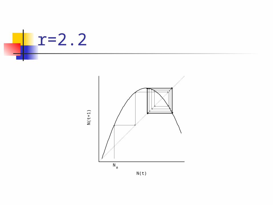
r=2.2

N(t)

N(t

+1)

N0

Chaotic behaviorr = 2.8

020406080

100120140

0 5 10 15 20

Time (t)

Po

pu

lati

on

siz

e (

N)

N0 = 50

N0 = 51

Predicting the future

0

100

200

300

400

0 50 100 150 200

Nt

Nt+1

Ricker model with K = 100 and r = 3.5

0

100

200

300

400

0 50 100 150 200

Nt

Nt+10

Model assumptions

Model assumptions

Increased density causes a (linear) decline in population growth rate

No variability in carrying capacity All other assumptions same as for

exponential growth (assume single, panmictic population, no age/stage structure)

Discrete Logistic Substitute b and d in

Nt+1 = RNt = (1+b - d) Nt

Nt+1 = Nt +[b0-aNt - d0-cNt]Nt

Rearrange and replace K = b0-d0 / (a+c)

1 1 tt t t

NN N rN

K