remote sensing

Article

Role of Climate Variability and Human Activity onPoopó Lake Droughts between 1990 and 2015Assessed Using Remote Sensing Data

Frédéric Satgé 1,2,*, Raúl Espinoza 3, Ramiro Pillco Zolá 4, Henrique Roig 1,2, Franck Timouk 5,Jorge Molina 4, Jérémie Garnier 1,2, Stéphane Calmant 2,6, Frédérique Seyler 2,7 andMarie-Paule Bonnet 2,7

1 Instituto de Geociência (IG), Universidade de Brasília, 70910-900 Brasilia-DF, Brazil; roig@unb.br (H.R.);garnier@unb.br (J.G.)

2 Mixed Laboratory International, Observatory for Environmental Change (LMI-OCE), IRD/UnB,Campus Darcy Ribeiro, 70910-900 Brasília, Brazil; stephane.calmant@ird.fr (S.C.);frederique.seyler@ird.fr (F.S.); marie-paule.bonnet@ird.fr (M.P.B.)

3 Laboratorio de Teledetección (LABTEL), Universidad Nacional Mayor de San Marcos, 15081 Lima, Peru;respinozavillar@gmail.com

4 Instituto de Hidráulica e Hidrología (IHH), Universidad Mayor de San Andrés, La Paz, Bolivia;rami_lund99@hotmail.com (R.P.Z.); amolina@umsa.bo (J.M.)

5 Géosciences Environnement Toulouse (GET) (IRD, CNRS), Université Paul Sabatier, 31062 Toulouse, France;franck.timouk@ird.fr

6 Laboratoire d’Etudes en Géophysique et Océanographie Spatiales (LEGOS) (UMR 5564, IRD, CNES, CNRS),Université Paul Sabatier, 31062 Toulouse, France

7 Espace Développement (ESPACE-DEV) (UMR 228, IRD), 34000 Montpellier, France* Correspondence: frederic.satge@gmail.com; Tel.: +55-61-3107-6626

Academic Editors: Alfredo R. Huete and Prasad S. ThenkabailReceived: 5 December 2016; Accepted: 25 February 2017; Published: 28 February 2017

Abstract: In 2015, an emergency state was declared in Bolivia when Poopó Lake dried up. Climatevariability and the increasing need for water are potential factors responsible for this situation.Because field data are missing over the region, no statements are possible about the influence ofmentioned factors. This study is a preliminary step toward the understanding of Poopó Lake droughtusing remote sensing data. First, atmospheric corrections for Landsat (FLAASH and L8SR), sevensatellite derived indexes for extracting water bodies, MOD16 evapotranspiration, PERSIANN-CDRand MSWEP rainfall products potentiality were assessed. Then, the fluctuations of Poopó Lake extentover the last 26 years are presented for the first time jointly, with the mean regional annual rainfall.Three main droughts are highlighted between 1990 and 2015: two are associated with negative annualrainfall anomalies in 1994 and 1995 and one associated with positive annual rainfall anomaly in2015. This suggests that other factors than rainfall influenced the recent disappearance of the lake.The regional evapotranspiration increased by 12.8% between 2000 and 2014. Evapotranspirationincrease is not homogeneous over the watershed but limited over the main agriculture regions.Agriculture activity is one of the major factors contributing to the regional desertification and recentdisappearance of Poopó Lake.

Keywords: Poopó Lake; drought; Landsat; Atmospheric correction; MOD16; PERSIANN-CDR; MSWEP

1. Introduction

The recent drought at Poopó Lake, the second largest water body in Bolivia, is of majorsocio-environmental concern as it condemned local population dependent on fishing activities jointly

Remote Sens. 2017, 9, 218; doi:10.3390/rs9030218 www.mdpi.com/journal/remotesensing

Remote Sens. 2017, 9, 218 2 of 17

with local endemic species. Moreover, the sediments contaminated by intense regional miningactivities trapped in the lake bottom were exposed to wind erosion, threatening the Altiplano regionwith contamination. Thus, there is the necessity of providing efficient and consistent surface watermonitoring tools for anticipating such crises and giving support for more sustainable use of waterresource in this region. Two main factors can be pointed out to explain the recent lake total drought:global warming and water consumption increase. Actually, the region suffers from continuouslyincreasing air temperatures of 0.15 to 0.25 ◦C over the last decades [1,2] from 1965 to 2012. Thistemperature increase has had a slight impact on evapotranspiration but has accelerated glaciermelting [3]. Some glaciers already disappeared. For example, the Chacaltaya Glacier, which was oneof the largest glaciers in the region, entirely melted in 2010 [4]. The shrinkage and disappearanceof glaciers obviously reduces the replenishment of water resources (surficial and subterranean),especially during the dry season [5]. In addition to climatic factors, some anthropic factors may directlyaffect Poopó Lake. Water extraction to sustain increasing mining activity, human populations (forconsumption) and agriculture kept rising over the last decades. Actually, the area of quinoa culture inBolivia increased from 38,800 to 70,000 ha from 1990 to 2012 [6] in response to the world’s demandsfor quinoa and its increasing price. Progressively, the replacement of native vegetation by quinoa hasaccelerated the desertification process across the region [7,8]. As the outlet of its own watershed, thePoopó Lake extent fluctuation is sensitive to climate change and increasing anthropic water demandsalong the watershed. With more than 25 years of land observations using different spectral bandsand considering replicates of 16 days, Landsat imagery collection is very suitable for monitoringvariations in lake coverage and for support decision for more sustainable use of water resources in thefuture. However, the electromagnetic radiation signals collected by satellites in the solar spectrum aremodified because they are scattered and absorbed by gazes and aerosols as they travel from the earth’ssurface to the sensor. Atmospheric correction is arguably the most important step in pre-processingLandsat data to monitor change detection when considering multitemporal time series images [9–11]but not when working on single date [11]. Today, the United States Geological Survey (USGS) serviceprovides an atmospherically corrected version of each LandSat scene: the Landsat Surface Reflectance(LSR) product. Here, we used field spectral measurement to quickly assess LSR estimates for theLandsat-8 OLI products for the first time over the Altiplano. The Surface Reflectances (SRs) obtainedafter applying the fast line-of-sight atmospheric analysis of spectral hypercubes (FLAASH) atmosphericcorrection were also considered for comparisons.

The method used to build a time series of the fluctuations of lake extent is based on detectingchanges in the pixel’s state from one Landsat scene to another. In the literature, several satellitederived indexes (SDIs) are proposed to separate water and land pixels. Depending on the region, oneSDI can be more suitable than another for delineating water bodies, and an SDI should be chosencarefully to produce realistic results [12,13]. However, in most studies, choosing the SDI remainsarbitrary or is based on the results of studies conducted in supposedly similar regions [14–17]. Here, wecompared the results obtained from the Normalized Difference Water Index (NDWI), Modified NDWI(MNDWI), Water Ratio Index (WRI), Normalized Difference Moisture Index (NDVI), Automated WaterExtraction Index (AWEI), Normalized Burn Ratio (NBR) and Land Surface Water Index (LSWI) withfield observations to provide general guidelines for potential users over the Altiplano region.

Finally, based on the most efficient Atmospheric model correction and SDI, a 26-year temporalseries from 1990 to the 2015 disappearance of the lake is presented for the first time. Aftervalidation, the MOD16 evapotranspiration (ET) products, the Precipitation Estimation from RemotelySensed Information Using Artificial Neural Networks–Climate Data Record (PERSIANN-CDR) andMulti-Source Weighted-Ensemble Precipitation (MSWEP) reanalysis rainfall products are confronted tothe Poopó Lake extent fluctuations. Rainfall and ET general trends are used to understand the potentialinfluence of the climatic variability and increasing irrigated quinoa culture over the watershed duringthe last decades. This study provides a preliminary analysis of the hydrological behavior of Poopó

Remote Sens. 2017, 9, 218 3 of 17

Lake over the last decades and could be used as a guideline by national authority to consider moresustainable use of water resources over the region.

2. Materials and Methods

2.1. Study Area

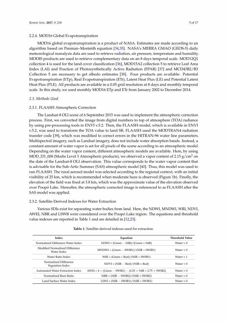
Poopó Lake is located on the southern part of the Andean Plateau in Bolivia between latitudes17◦S and 20◦S and longitudes 66◦W and 68◦W and with a mean elevation of 3686 m (Figure 1a).Poopó Lake is the second largest lake in Bolivia, covering an area of 500 to 3000 km2 at its lowestand highest levels, respectively [17]. The extent of Poopó Lake drastically changes between wet anddry seasons because the region where the lake is located is very flat [18]. The only outflow of thelake is through the Lakajawuira River on the southern end of the lake, which rarely flows towardsthe Coipasa Salar. In the last 50 years, this river only flooded once in 1986 [17]. Thus, Poopó Lake isconsidered a terminal point of the endorheic Altiplano system [17]. The Poopó Lake region is arid, witha mean annual precipitation of approximately 400 mm over the lake [19] and a high evapotranspirationrate [20]. According to pan evaporation measurement, the potential evaporation was estimated at1700 mm/year [17] and resulted in extremely saline water. Regarding the local population, the lakeis of primordial importance because people depend on it for fishing and agricultural activities [7,8].In December 2015, a national emergency alert was launched by the national authority in Bolivia afterthe lake totally dried up. This situation directly impacted the ecosystem and the population livingaround the lake.

Remote Sens. 2017, 9, 218 3 of 17

2. Materials and Methods

2.1. Study Area

Poopó Lake is located on the southern part of the Andean Plateau in Bolivia between latitudes 17°S and 20°S and longitudes 66°W and 68°W and with a mean elevation of 3686 m (Figure 1a). Poopó Lake is the second largest lake in Bolivia, covering an area of 500 to 3000 km2 at its lowest and highest levels, respectively [17]. The extent of Poopó Lake drastically changes between wet and dry seasons because the region where the lake is located is very flat [18]. The only outflow of the lake is through the Lakajawuira River on the southern end of the lake, which rarely flows towards the Coipasa Salar. In the last 50 years, this river only flooded once in 1986 [17]. Thus, Poopó Lake is considered a terminal point of the endorheic Altiplano system [17]. The Poopó Lake region is arid, with a mean annual precipitation of approximately 400 mm over the lake [19] and a high evapotranspiration rate [20]. According to pan evaporation measurement, the potential evaporation was estimated at 1700 mm/year [17] and resulted in extremely saline water. Regarding the local population, the lake is of primordial importance because people depend on it for fishing and agricultural activities [7,8]. In December 2015, a national emergency alert was launched by the national authority in Bolivia after the lake totally dried up. This situation directly impacted the ecosystem and the population living around the lake.

Figure 1. Study area of the watershed (a); and Landsat-8 OLI scene from 6 September 2014, with the ground control points (GCPs) locations (b).

2.2. Data Used

2.2.1. Field Spectral Measurements

Spectral radiometric measurements were acquired from the field, using TriOS RAMSES Sensors on 6 September 2014. A total of 69 points from 5 transects located on the north, east, south and west lakeshores and in the shallow part of the lake were analyzed (Figure 1b). At each point, the lake depth and SR in the spectral domain between 450 and 950 nm were registered. These data were acquired

Figure 1. Study area of the watershed (a); and Landsat-8 OLI scene from 6 September 2014, with theground control points (GCPs) locations (b).

Remote Sens. 2017, 9, 218 4 of 17

2.2. Data Used

2.2.1. Field Spectral Measurements

Spectral radiometric measurements were acquired from the field, using TriOS RAMSES Sensorson 6 September 2014. A total of 69 points from 5 transects located on the north, east, south and westlakeshores and in the shallow part of the lake were analyzed (Figure 1b). At each point, the lake depthand SR in the spectral domain between 450 and 950 nm were registered. These data were acquiredusing the methodology established by [21]. Hereafter, we refer to Ground Control Points (GCPs) whenreferring to the in situ measurements. Spectral radiometric and Landsat measurement differ in term ofspatial resolution (point vs. Pixel). This is an important feature to be considered to avoid inconsistentcomparison. To account for this, spectral radiometric measurements were done on homogeneous areain term of water depth and water–soil representation to avoid mixed pixel. As Poopó region is a veryflat region, and Landsat pixel length is of approximately 30 m, it was easy to find homogeneous areasall around the lake. Recorded values were resampled to match Landsat OLI 8 blue, green, red and nearinfra-red (NIR) bands. The Landsat Quality Assessment (QA) band provides the bit-packed values ofthe surface, atmosphere and sensor conditions that can affect the reflectance measured at each pixelof the considered scene. According to the QA band, 13 points were dismissed because of clouds orcirrus cover and 56 points were available for comparisons. Landsat reflectance measurements aregiven per unit area, while TriOS RAMSES measurements provide reflectance values per unit solidangle (Steradian). Thus, field spectral measurements were multiplied by the π value to match theLandsat reflectance value.

2.2.2. Landsat Imagery

The Landsat-8 satellite was launched in February 2013 with OLI and Thermal Infra-Red Sensor(TIRS) instruments on board. OLI, ETM+, ETM and TM sensors have different bandwidths that couldcompromise their compatibility. Regarding the OLI and ETM+, good radiometric compatibility wasfound between their respective bands [22] and can be used as complementary data [23]. OLI wasfound to largely inherit the band-pass characteristics of ETM+ and achieve continuity of Landsatdata [24]. On the other hand, TM and ETM + were found to exhibit excellent data continuity [25], andthe measurements of SR obtained by these sensors could be combined with minimal error withoutsacrificing product accuracy [26–28]. Based on these observations, it is possible to use OLI, ETM+and TM jointly to retrieve long temporal series or series with increased observation frequencies.Each Landsat scene is available in an atmospherically corrected format called the LSR product andfreely available from the USGS. For the Landsat TM, ETM and ETM+, the specialized LandsatEcosystem Disturbance Adaptive Processing System (LEDAPS) software [29] and the specializedL8SR software [30] are used to retrieve the SR for Landsat TM, ETM and ETM+ and Landsat-8OLI, respectively.

2.2.3. Satellite Rainfall Estimates

Two reanalysis rainfall products named PERSIANN-CDR [31] and MSWEP [32] were consideredto cover the whole 1990–2016 period. PERSIANN-CDR was released in 2014 by the National ClimaticData Center (NCDC) Climate Data Record (CDR) program of the National Oceanic and AtmosphericAdministration (NOAA). PERSIANN-CDR covers the 1983 to 2015 period providing daily rainfallestimate on a 0.25◦ spatial resolution. MSWEP was released in 2016 [32] and covers the 1979–2015period with daily rainfall data on a 0.25◦ spatial resolution. MSWEP estimates are based on the ClimateHazards Group Precipitation Climatology (CHPclim) dataset (0.05◦) [33]. Additionally, precipitationanomalies from gauge observation, satellite rainfall estimates and atmospheric model reanalysis areused to fix MSWEP estimates temporal variability.

Remote Sens. 2017, 9, 218 5 of 17

2.2.4. MOD16 Global Evapotranspiration

MOD16 global evapotranspiration is a product of NASA. Estimates are made according to analgorithm based on Penman–Monteith equation [34,35]. NASA’s MERRA GMAO (GEOS-5) dailymeteorological reanalysis data are used to retrieve radiation, air pressure, temperature and humidity.MODIS products are used to retrieve complementary data on an 8 days temporal scale. MOD12Q1collection 4 is used for the land cover classification [36], MOD15A2 collection 5 to retrieve Leaf AreaIndex (LAI) and Fraction of Photosynthetically Active Radiation (FPAR) [37] and MCD43B2/B3Collection 5 are necessary to get albedo estimates [38]. Four products are available: PotentialEvapotranspiration (ETp), Real Evapotranspiration (ETr), Latent Heat Flux (LE) and Potential LatentHeat Flux (PLE). All products are available in a 0.05 grid resolution at 8 days and monthly temporalscale. In this study, we used monthly MOD16 ETp and ETr from January 2002 to December 2014.

2.3. Methods Used

2.3.1. FLAASH Atmospheric Correction

The Landsat-8 OLI scene of 6 September 2015 was used to implement the atmospheric correctionprocess. First, we converted the image from digital numbers to top of atmosphere (TOA) radianceby using pre-processing tools in ENVI v.5.2. Then, the FLAASH model, which is available in ENVIv.5.2, was used to transform the TOA value to land SR. FLAASH used the MODTRAN4 radiationtransfer code [39], which was modified to correct errors in the HITRAN-96 water line parameters.Multispectral imagery, such as Landsat imagery, does not include water absorption bands. Instead, aconstant amount of water vapor is set for all pixels of the scene according to an atmospheric model.Depending on the water vapor content, different atmospheric models are available. Here, by usingMOD_D3_008 (Modis Level 3 Atmospheric products), we observed a vapor content of 2.15 g/cm2 onthe date of the Landsat-8 OLI observation. This value corresponds to the water vapor content thatis advisable for the Sub-Artic Summer (SAS) atmospheric model [40]. Thus, this model was used torun FLAASH. The rural aerosol model was selected according to the regional context, with an initialvisibility of 25 km, which is recommended when moderate haze is observed (Figure 1b). Finally, theelevation of the field was fixed at 3.8 km, which was the approximate value of the elevation observedover Poopó Lake. Hereafter, the atmospheric corrected image is referenced to as FLAASH after theSAS model was applied.

2.3.2. Satellite-Derived Indexes for Water Extraction

Various SDIs exist for separating water bodies from land. Here, the NDWI, MNDWI, WRI, NDVI,AWEI, NBR and LSWR were considered over the Poopó Lake region. The equations and thresholdvalue indexes are reported in Table 1 and are detailed in [12,23].

Table 1. Satellite-derived indexes used for extraction.

Index Equation Threshold Value

Normalized Difference Water Index NDWI = (Green − NIR)/(Green + NIR) Water > 0

Modified Normalized DifferenceWater Index MNDWI = (Green − SWIR1)/(NIR + SWIR1) Water > 0

Water Ratio Index WRI = (Green + Red)/(NIR + SWIR1) Water > 1

Normalized DifferenceVegetation Index NDVI = (NIR − Red)/(NIR + Red) Water < 0

Automated Water Extraction Index AWEI = 4 × (Green − SWIR1) − (0.25 × NIR + 2.75 × SWIR2) Water > 0

Normalized Burn Ratio NBR = (NIR − SWIR2)/(NIR + SWIR2) Water > 0

Land Surface Water Index LSWI = (NIR − SWIR1)/(NIR + SWIR1) Water > 0

Remote Sens. 2017, 9, 218 6 of 17

2.4. Assessment of Data and Method

2.4.1. L8SR and FLAASH Assessment

At each GCPs location, field spectral measurement, FLAASH, LSR and Landsat SR value forBlue, Green, Red and NIR were extracted to build the database. Comparisons between field spectralmeasurement and FLAASH, LSR and Landsat SR were made considering all single band values (red,blue, green and near infra-red) and possible band ratios (green/red, blue/green, red/blue, blue/nearinfra-red, green/near infra-red, and red/near infra-red) (Table 2). Landsat reflectance value wasconsidered to observe the enhancements of the SR estimations gained through the L8SR and FLAASHprocesses. The band ratios are considered to observe the relative errors between bands. Indeed, lowerror in band ratio implies that the trend between the concerned bands is well represented. Consideringall GCPs, the Mean Error (ME), Root Mean Square Error (RMSE) and Correlation Coefficient (CC) werecomputed for all single and band ratios. Different ranges of values were observed for the differentbands and band ratios, which complicated the interpretation of the absolute errors. Thus, the ME andRMSE were divided by the average GCP value to obtain the relative statistic error percentage (%MEand %RMSE) (Table 2).

Table 2. %ME, %RMSE and CC for the SR measured by Landsat (uncorrected), FLAASH SAS and LSRin comparison with in situ field measurements.

ME (%) RMSE (%) CC

Landsat FLAASH LSR Landsat FLAASH LSR Landsat FLAASH LSR

Blue 0.0 −0.9 −0.9 48.4 109.2 110.9 0.92 0.93 0.91Green −0.2 −0.9 −0.9 44.0 102.7 103.7 0.91 0.92 0.91Red −0.2 −0.9 −0.9 45.2 103.4 104.0 0.91 0.91 0.91

Near IR −0.1 −0.9 −0.9 57.8 115.1 115.6 0.84 0.84 0.84Green/Red 0.0 0.0 0.0 13.1 5.0 6.5 0.94 0.98 0.97Blue/Green 0.4 0.1 0.0 38.6 9.4 12.4 0.47 0.88 0.69Red/Blue −0.3 0.0 0.0 41.9 10.9 15.6 0.75 0.96 0.89

Blue/Infra-Red −0.5 −0.1 −4.0 122.1 46.3 2663.3 0.90 0.93 −0.35Red/Infra-Red −0.6 −0.1 −3.8 118.5 45.3 2512.3 0.87 0.92 −0.37Green/Infra-Red −0.7 −0.1 −4.4 137.2 50.1 2896.3 0.88 0.93 −0.38

2.4.2. SDI Assessment

Poopó Lake is a very shallow lake. In shallow part, light penetration in water column is veryhigh. Thus, SR is highly influenced by Lake Bottom response complicating water/land separation.To account for this feature, we divided the GCPs into 4 classes corresponding to “water”, “veryshallow water”, “interconnected water”, and “soil”. The classes contained 26, 16, 5 and 9 GCPs,respectively. The “Very shallow water” and “water” classes had water depths ranging from 0 to 5 cmand superior to 5 cm, respectively. The “interconnected water” class corresponded to mixed pixelswith interconnected water units. At each pixel location, including a GCP, the SDI values from themost accurate scenes in term of the SR estimation were compared with field observations. Two casesare possible: SDI value and field observations agreed or SDI value and field observations disagreed(Table 3). Outlier values were observed when the SDI failed to correctly identify the field observations(Table 3, Figure 2). A large number of outliers mean that the considered SDI was poorly efficientover the region. SDIs potentiality is generally more effective after the threshold value was adjusted.Here, for each considered SDI, we proposed an adjusted threshold to minimize as possible the outliernumber. For each SDI, the number of outliers was computed before and after the threshold adjustment(Table 4). Finally, we computed the extent of Poopó Lake based on each SDI using the default andadjusted threshold values (Table 4).

Remote Sens. 2017, 9, 218 7 of 17

Table 3. Assessment of SDI over Poopó Lake. Water refers to “water” and “very shallow water” classes,and Land refers to “interconnected water” and “soil” classes.

SDI Observation

Water LandField

ObservationWater Ok OutlierLand Outlier Ok

Remote Sens. 2017, 9, 218 6 of 17

FLAASH processes. The band ratios are considered to observe the relative errors between bands. Indeed, low error in band ratio implies that the trend between the concerned bands is well represented. Considering all GCPs, the Mean Error (ME), Root Mean Square Error (RMSE) and Correlation Coefficient (CC) were computed for all single and band ratios. Different ranges of values were observed for the different bands and band ratios, which complicated the interpretation of the absolute errors. Thus, the ME and RMSE were divided by the average GCP value to obtain the relative statistic error percentage (%ME and %RMSE) (Table 1).

Figure 2. Categorical statistical analysis of SDI. Solid vertical lines represent the advocated thresholds, and the outliers are shown in red.

Table 2. %ME, %RMSE and CC for the SR measured by Landsat (uncorrected), FLAASH SAS and LSR in comparison with in situ field measurements.

ME (%) RMSE (%) CC Landsat FLAASH LSR Landsat FLAASH LSR Landsat FLAASH LSR

Blue 0.0 −0.9 −0.9 48.4 109.2 110.9 0.92 0.93 0.91 Green −0.2 −0.9 −0.9 44.0 102.7 103.7 0.91 0.92 0.91 Red −0.2 −0.9 −0.9 45.2 103.4 104.0 0.91 0.91 0.91

Near IR −0.1 −0.9 −0.9 57.8 115.1 115.6 0.84 0.84 0.84 Green/Red 0.0 0.0 0.0 13.1 5.0 6.5 0.94 0.98 0.97 Blue/Green 0.4 0.1 0.0 38.6 9.4 12.4 0.47 0.88 0.69 Red/Blue −0.3 0.0 0.0 41.9 10.9 15.6 0.75 0.96 0.89

Blue/Infra-Red −0.5 −0.1 −4.0 122.1 46.3 2663.3 0.90 0.93 −0.35Red/Infra-Red −0.6 −0.1 −3.8 118.5 45.3 2512.3 0.87 0.92 −0.37

Green/Infra-Red −0.7 −0.1 −4.4 137.2 50.1 2896.3 0.88 0.93 −0.38

2.4.2. SDI Assessment

Poopó Lake is a very shallow lake. In shallow part, light penetration in water column is very high. Thus, SR is highly influenced by Lake Bottom response complicating water/land separation. To

Figure 2. Categorical statistical analysis of SDI. Solid vertical lines represent the advocated thresholds,and the outliers are shown in red.

Table 4. SDI outliers for the default and adjusted threshold values with the corresponding superficialextents of Poopó Lake on 22 September 2014.

SDI DefaultThreshold Value

OutlierNumber

Superficial(km2)

RecommendedThreshold Value

OutlierNumber

Superficial(km2)

NDWI 0 14 1204 −0.0235 12 1314MNDWI 0 6 1664 0.15 3 1477

WRI 1 4 1570 1.05 3 1497NDVI 0 7 1160 0.025 6 1208AWEI 0 4 1454 −0.1 3 1454NBR 0 13 2627 0.21 7 1906LSWI 0 10 2099 0.05 6 1820

2.4.3. Satellite Rainfall and MOD16 Evapotranspiration Estimates Assessment

The mean regional monthly rainfall series was computed for both PERSIANN-CDR and MSWEPfor the 1998–2014 period aggregating all pixels included into the watershed. Another mean regionalmonthly series was computed by meaning PERSIANN-CDR and MSWEP rainfall series (called MERGEhereafter). The three series were compared to a mean reference regional monthly series derived fromthe Multisatellite Precipitation Analysis 3B42 (TMPA-3B42) v.7 for the same period. TMPA-3B42 v.7 can

Remote Sens. 2017, 9, 218 8 of 17

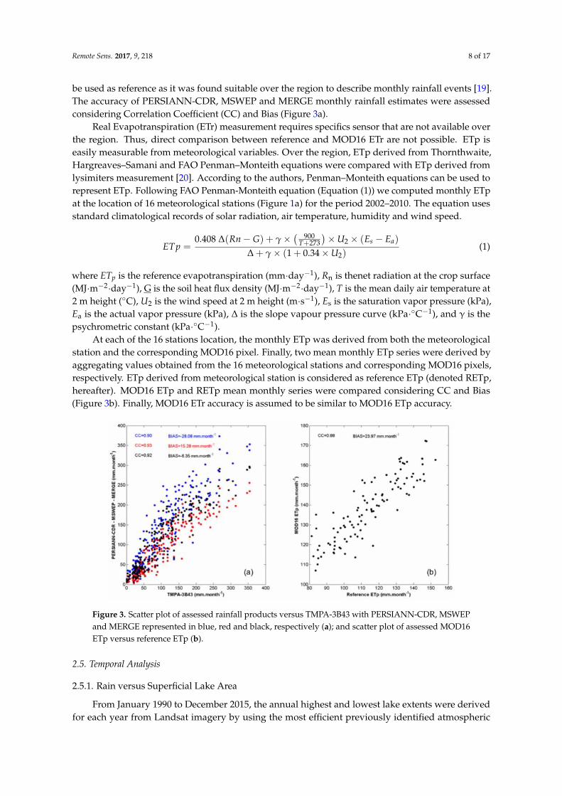
be used as reference as it was found suitable over the region to describe monthly rainfall events [19].The accuracy of PERSIANN-CDR, MSWEP and MERGE monthly rainfall estimates were assessedconsidering Correlation Coefficient (CC) and Bias (Figure 3a).

Real Evapotranspiration (ETr) measurement requires specifics sensor that are not available overthe region. Thus, direct comparison between reference and MOD16 ETr are not possible. ETp iseasily measurable from meteorological variables. Over the region, ETp derived from Thornthwaite,Hargreaves–Samani and FAO Penman–Monteith equations were compared with ETp derived fromlysimiters measurement [20]. According to the authors, Penman–Monteith equations can be used torepresent ETp. Following FAO Penman-Monteith equation (Equation (1)) we computed monthly ETpat the location of 16 meteorological stations (Figure 1a) for the period 2002–2010. The equation usesstandard climatological records of solar radiation, air temperature, humidity and wind speed.

ETp =0.408 ∆(Rn − G) + γ ×

( 900T+273

)× U2 × (Es − Ea)

∆ + γ × (1 + 0.34 × U2)(1)

where ETp is the reference evapotranspiration (mm·day−1), Rn is thenet radiation at the crop surface(MJ·m−2·day−1), G is the soil heat flux density (MJ·m−2·day−1), T is the mean daily air temperature at2 m height (◦C), U2 is the wind speed at 2 m height (m·s−1), Es is the saturation vapor pressure (kPa),Ea is the actual vapor pressure (kPa), ∆ is the slope vapour pressure curve (kPa·◦C−1), and γ is thepsychrometric constant (kPa·◦C−1).

At each of the 16 stations location, the monthly ETp was derived from both the meteorologicalstation and the corresponding MOD16 pixel. Finally, two mean monthly ETp series were derived byaggregating values obtained from the 16 meteorological stations and corresponding MOD16 pixels,respectively. ETp derived from meteorological station is considered as reference ETp (denoted RETp,hereafter). MOD16 ETp and RETp mean monthly series were compared considering CC and Bias(Figure 3b). Finally, MOD16 ETr accuracy is assumed to be similar to MOD16 ETp accuracy.

Remote Sens. 2017, 9, 218 8 of 17

0.408∆ 900273∆ 1 0.34 (1)

where ETp is the reference evapotranspiration (mm·day−1), Rn is thenet radiation at the crop surface (MJ·m−2·day−1), G is the soil heat flux density (MJ·m−2·day−1), T is the mean daily air temperature at 2 m height (°C), U2 is the wind speed at 2 m height (m·s−1), Es is the saturation vapor pressure (kPa), Ea is the actual vapor pressure (kPa), ∆ is the slope vapour pressure curve (kPa·°C−1), andγ is the psychrometric constant (kPa·°C−1).

Figure 3. Scatter plot of assessed rainfall products versus TMPA-3B43 with PERSIANN-CDR, MSWEP and MERGE represented in blue, red and black, respectively (a); and scatter plot of assessed MOD16 ETp versus reference ETp (b).

At each of the 16 stations location, the monthly ETp was derived from both the meteorological station and the corresponding MOD16 pixel. Finally, two mean monthly ETp series were derived by aggregating values obtained from the 16 meteorological stations and corresponding MOD16 pixels, respectively. ETp derived from meteorological station is considered as reference ETp (denoted RETp, hereafter). MOD16 ETp and RETp mean monthly series were compared considering CC and Bias (Figure 3b). Finally, MOD16 ETr accuracy is assumed to be similar to MOD16 ETp accuracy.

2.5. Temporal Analysis

2.5.1. Rain versus Superficial Lake Area

From January 1990 to December 2015, the annual highest and lowest lake extents were derived for each year from Landsat imagery by using the most efficient previously identified atmospheric correction processes and SDI. Attention was paid to only select almost cloud free Landsat TM, ETM or OLI scenes. Overall, 48 Landsat scenes were selected and used. From 2012, only Landsat ETM+ scenes are available. Over Poopó Lake, the Landsat ETM+ scenes are strongly impacted by the SLC failure that occurred on 31 May 2003. Thus, these data are not suitable for use in the study. Therefore 2 MODIS scenes were used to fill the gap. Using the MODIS scene to derive the extent of Poopó Lake is acceptable because a strong correlation was previously found between the extents of Poopó Lake derived from MODIS and Landsat data [14]. MODIS scenes are already atmospheric corrected and thus SDI can be directly applied. The fluctuation of the lake extent was compared with the mean regional annual rainfall evolution (Figure 4a). The mean rainfall was computed based on a hydrological year (November to October) and using MERGE rainfall product (Figure 4a).

Figure 3. Scatter plot of assessed rainfall products versus TMPA-3B43 with PERSIANN-CDR, MSWEPand MERGE represented in blue, red and black, respectively (a); and scatter plot of assessed MOD16ETp versus reference ETp (b).

2.5. Temporal Analysis

2.5.1. Rain versus Superficial Lake Area

From January 1990 to December 2015, the annual highest and lowest lake extents were derivedfor each year from Landsat imagery by using the most efficient previously identified atmospheric

Remote Sens. 2017, 9, 218 9 of 17

correction processes and SDI. Attention was paid to only select almost cloud free Landsat TM, ETMor OLI scenes. Overall, 48 Landsat scenes were selected and used. From 2012, only Landsat ETM+scenes are available. Over Poopó Lake, the Landsat ETM+ scenes are strongly impacted by the SLCfailure that occurred on 31 May 2003. Thus, these data are not suitable for use in the study. Therefore2 MODIS scenes were used to fill the gap. Using the MODIS scene to derive the extent of Poopó Lakeis acceptable because a strong correlation was previously found between the extents of Poopó Lakederived from MODIS and Landsat data [14]. MODIS scenes are already atmospheric corrected andthus SDI can be directly applied. The fluctuation of the lake extent was compared with the meanregional annual rainfall evolution (Figure 4a). The mean rainfall was computed based on a hydrologicalyear (November to October) and using MERGE rainfall product (Figure 4a). Additionally, the meanseasonal rainfall anomalies and lake extent anomalies for both dry and wet seasons were computedand compared (Figure 4b).

Remote Sens. 2017, 9, 218 9 of 17

Additionally, the mean seasonal rainfall anomalies and lake extent anomalies for both dry and wet seasons were computed and compared (Figure 4b).

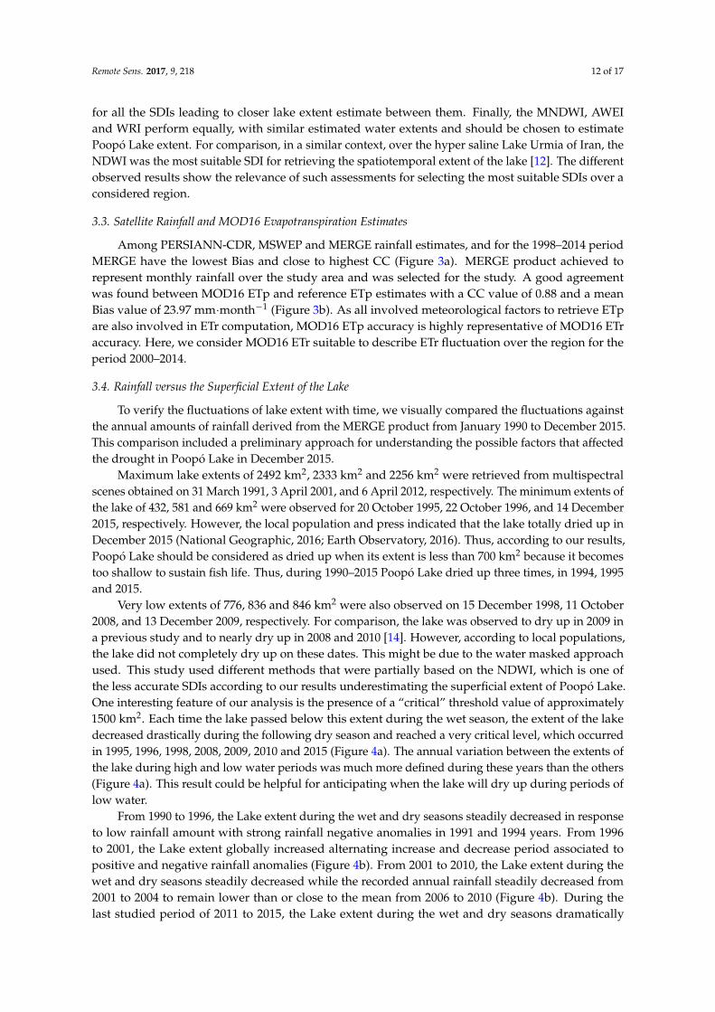
Figure 4. Extent of Poopó Lake (km2) and the variations of the MERGE seasonal amount of rainfall (mm) between 1990 and 2015 (a); and rainfall and lake extent anomalies (b). The maximum and minimum extents are plotted in blue and red, respectively.

2.5.2. ETr, ETp and Rainfall Tendency over the Last 15 Years

The monthly rainfall, ETp and ETr over Poopó Lake watershed for the period 2000–2014 are presented jointly with their global trend (Figure 5). The global trend is obtained from a simple linear regression of the mean monthly series. The Mann-Kendall (MK) test [41,42] was used to statistically verified if the monotonic trend in the mean monthly rainfall, ETp and ETr over the 2000–2014 period were significant. A MK p-value inferior to 0.05 corresponds to significant monotonic trend. Finally, to observe the ETr dynamic in space along the whole watershed, the mean monthly ETr series were computed at each MOD16 pixel location and its linear regression was used to compute the ETr changing rate from 2000–2014 (Equation (2)). Results are presented in Figure 6. Additionally, the MK p-value was computed at each MOD16 pixel according to the corresponding ETr series. Results are presented in Figure 6. 100

(2)

where ETr2014 and ETr2000 are the ETr computed from the linear regression of the considered MOD16 pixel for the years 2014 and 2000, respectively.

Finally, a multiple linear regression was used to check the relative influence of rain, ETp and ETr on the lake fluctuations for the 2000–2014 period. The annual lake extent during the dry season was considered as dependent variable while corresponding mean regional annual precipitation, ETp and ETr were considered as independent variables (predictors). The mean annual precipitation, ETp and ETr were computed for the corresponding season between May and March. It is noteworthy that we only considered lake extent fluctuation during the dry season. Actually, the lake extent during the wet season is controlled at 65% by Desaguadero River input and the rest by local Poopó Lake watershed input [17]. Thus, at the regional scale, the influences of rain, ETp and ETr are expected to be more significant during the dry season than during the wet season as Desaguadero River input is much smaller.

Figure 4. Extent of Poopó Lake (km2) and the variations of the MERGE seasonal amount of rainfall(mm) between 1990 and 2015 (a); and rainfall and lake extent anomalies (b). The maximum andminimum extents are plotted in blue and red, respectively.

2.5.2. ETr, ETp and Rainfall Tendency over the Last 15 Years

The monthly rainfall, ETp and ETr over Poopó Lake watershed for the period 2000–2014 arepresented jointly with their global trend (Figure 5). The global trend is obtained from a simple linearregression of the mean monthly series. The Mann-Kendall (MK) test [41,42] was used to statisticallyverified if the monotonic trend in the mean monthly rainfall, ETp and ETr over the 2000–2014 periodwere significant. A MK p-value inferior to 0.05 corresponds to significant monotonic trend. Finally,to observe the ETr dynamic in space along the whole watershed, the mean monthly ETr series werecomputed at each MOD16 pixel location and its linear regression was used to compute the ETr changingrate from 2000–2014 (Equation (2)). Results are presented in Figure 6. Additionally, the MK p-valuewas computed at each MOD16 pixel according to the corresponding ETr series. Results are presentedin Figure 6.

Changing Rate =(ETr2014 − ETr2000)× 100

ETr2000(2)

where ETr2014 and ETr2000 are the ETr computed from the linear regression of the considered MOD16pixel for the years 2014 and 2000, respectively.

Finally, a multiple linear regression was used to check the relative influence of rain, ETp andETr on the lake fluctuations for the 2000–2014 period. The annual lake extent during the dry seasonwas considered as dependent variable while corresponding mean regional annual precipitation, ETpand ETr were considered as independent variables (predictors). The mean annual precipitation, ETp

Remote Sens. 2017, 9, 218 10 of 17

and ETr were computed for the corresponding season between May and March. It is noteworthy thatwe only considered lake extent fluctuation during the dry season. Actually, the lake extent duringthe wet season is controlled at 65% by Desaguadero River input and the rest by local Poopó Lakewatershed input [17]. Thus, at the regional scale, the influences of rain, ETp and ETr are expected tobe more significant during the dry season than during the wet season as Desaguadero River input ismuch smaller.Remote Sens. 2017, 9, 218 10 of 17

Figure 5. Monthly rain, ETp and ETr derived from MERGE and MOD16 for the 2000–2014 period (a); and their general trend over the same period with the Man Kendal p-value (b).

Figure 6. ETr increase rate for the 2000–2014 period and corresponding MK p-value.

Figure 5. Monthly rain, ETp and ETr derived from MERGE and MOD16 for the 2000–2014 period (a);and their general trend over the same period with the Man Kendal p-value (b).

Remote Sens. 2017, 9, 218 10 of 17

Figure 5. Monthly rain, ETp and ETr derived from MERGE and MOD16 for the 2000–2014 period (a); and their general trend over the same period with the Man Kendal p-value (b).

Figure 6. ETr increase rate for the 2000–2014 period and corresponding MK p-value.

Figure 6. ETr increase rate for the 2000–2014 period and corresponding MK p-value.

Remote Sens. 2017, 9, 218 11 of 17

3. Results and Discussion

3.1. Effects of Atmospheric Correction

Using a single band approach and for all considered bands, the Landsat SR estimate was generallycloser to the field SR measurements than the LSR and FLAASH SR with %ME and %RMSE close to 0.FLAASH and LSR resulted in underestimations of SR with negative bias values. When consideringthe band ratio, the FLAASH and LSR SR estimations were closer to the field SR than the Landsat SRestimates with %ME closer to 0 and lower RMSE value. The corrected LSR and FLAASH data tendedto result in more homogeneous relative trends between the bands than the uncorrected data. Indeed,for all band ratios, the error distribution was closer to 0 for the LSR and FLAASH scenes than for theLandsat scene, which presented greater error distributions.

The NIR band is the most affected by atmospheric absorption and scattering. This band presentedlower CCs and higher %RMSEs and %MEs. Consequently, all band ratios including the NIR bandpresented highest %RMSE values (Table 2). In the case of FLAASH correction, the %RMSE was5–10 times higher than that of the other ratio (Table 2). This difference was even greater whenconsidering the LSR products with very high %RMSEs for the band ratios including the NIR band.This difference results from the strong underestimation of the NIR with some negative value observed.This LSR inconsistency seems to reoccur because negative values in NIR bands were also observedin the LSR scenes from 21 August and 22 September 2014 as well as over Brazilian water bodies atdifferent date. Although FLAASH also underestimates the NIR SR value, it had a lower impact becauseno negative value was observed.

Using the single band approach, atmospheric correction degraded the SR estimation becauselower %ME and %RMSE values were found before atmospheric correction was applied. However,the opposite trend was observed when considering the band ratios. FLAASH Atmospheric correctionenhanced the relative error between the bands, with %RMSE reduction by a factor of 3, higher CCsand lower %MEs for all of the considered band ratios. Thus, over Poopó Lake, FLAASH correction ismore suitable than the L8SR algorithm. SDIs are based on band combination and thus their efficiencyhighly relies on relative band error. As the study aimed to use SDI to retrieve lake extent, we used theFLAASH correction to build the Landsat scene database for the 1990–2015 period.

3.2. SDI Assessment

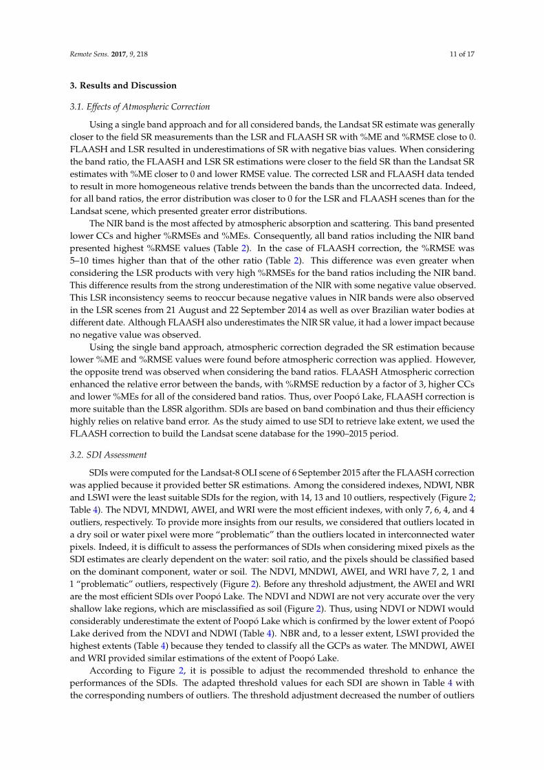
SDIs were computed for the Landsat-8 OLI scene of 6 September 2015 after the FLAASH correctionwas applied because it provided better SR estimations. Among the considered indexes, NDWI, NBRand LSWI were the least suitable SDIs for the region, with 14, 13 and 10 outliers, respectively (Figure 2;Table 4). The NDVI, MNDWI, AWEI, and WRI were the most efficient indexes, with only 7, 6, 4, and 4outliers, respectively. To provide more insights from our results, we considered that outliers located ina dry soil or water pixel were more “problematic” than the outliers located in interconnected waterpixels. Indeed, it is difficult to assess the performances of SDIs when considering mixed pixels as theSDI estimates are clearly dependent on the water: soil ratio, and the pixels should be classified basedon the dominant component, water or soil. The NDVI, MNDWI, AWEI, and WRI have 7, 2, 1 and1 “problematic” outliers, respectively (Figure 2). Before any threshold adjustment, the AWEI and WRIare the most efficient SDIs over Poopó Lake. The NDVI and NDWI are not very accurate over the veryshallow lake regions, which are misclassified as soil (Figure 2). Thus, using NDVI or NDWI wouldconsiderably underestimate the extent of Poopó Lake which is confirmed by the lower extent of PoopóLake derived from the NDVI and NDWI (Table 4). NBR and, to a lesser extent, LSWI provided thehighest extents (Table 4) because they tended to classify all the GCPs as water. The MNDWI, AWEIand WRI provided similar estimations of the extent of Poopó Lake.

According to Figure 2, it is possible to adjust the recommended threshold to enhance theperformances of the SDIs. The adapted threshold values for each SDI are shown in Table 4 withthe corresponding numbers of outliers. The threshold adjustment decreased the number of outliers

Remote Sens. 2017, 9, 218 12 of 17

for all the SDIs leading to closer lake extent estimate between them. Finally, the MNDWI, AWEIand WRI perform equally, with similar estimated water extents and should be chosen to estimatePoopó Lake extent. For comparison, in a similar context, over the hyper saline Lake Urmia of Iran, theNDWI was the most suitable SDI for retrieving the spatiotemporal extent of the lake [12]. The differentobserved results show the relevance of such assessments for selecting the most suitable SDIs over aconsidered region.

3.3. Satellite Rainfall and MOD16 Evapotranspiration Estimates

Among PERSIANN-CDR, MSWEP and MERGE rainfall estimates, and for the 1998–2014 periodMERGE have the lowest Bias and close to highest CC (Figure 3a). MERGE product achieved torepresent monthly rainfall over the study area and was selected for the study. A good agreementwas found between MOD16 ETp and reference ETp estimates with a CC value of 0.88 and a meanBias value of 23.97 mm·month−1 (Figure 3b). As all involved meteorological factors to retrieve ETpare also involved in ETr computation, MOD16 ETp accuracy is highly representative of MOD16 ETraccuracy. Here, we consider MOD16 ETr suitable to describe ETr fluctuation over the region for theperiod 2000–2014.

3.4. Rainfall versus the Superficial Extent of the Lake

To verify the fluctuations of lake extent with time, we visually compared the fluctuations againstthe annual amounts of rainfall derived from the MERGE product from January 1990 to December 2015.This comparison included a preliminary approach for understanding the possible factors that affectedthe drought in Poopó Lake in December 2015.

Maximum lake extents of 2492 km2, 2333 km2 and 2256 km2 were retrieved from multispectralscenes obtained on 31 March 1991, 3 April 2001, and 6 April 2012, respectively. The minimum extents ofthe lake of 432, 581 and 669 km2 were observed for 20 October 1995, 22 October 1996, and 14 December2015, respectively. However, the local population and press indicated that the lake totally dried up inDecember 2015 (National Geographic, 2016; Earth Observatory, 2016). Thus, according to our results,Poopó Lake should be considered as dried up when its extent is less than 700 km2 because it becomestoo shallow to sustain fish life. Thus, during 1990–2015 Poopó Lake dried up three times, in 1994, 1995and 2015.

Very low extents of 776, 836 and 846 km2 were also observed on 15 December 1998, 11 October2008, and 13 December 2009, respectively. For comparison, the lake was observed to dry up in 2009 ina previous study and to nearly dry up in 2008 and 2010 [14]. However, according to local populations,the lake did not completely dry up on these dates. This might be due to the water masked approachused. This study used different methods that were partially based on the NDWI, which is one ofthe less accurate SDIs according to our results underestimating the superficial extent of Poopó Lake.One interesting feature of our analysis is the presence of a “critical” threshold value of approximately1500 km2. Each time the lake passed below this extent during the wet season, the extent of the lakedecreased drastically during the following dry season and reached a very critical level, which occurredin 1995, 1996, 1998, 2008, 2009, 2010 and 2015 (Figure 4a). The annual variation between the extents ofthe lake during high and low water periods was much more defined during these years than the others(Figure 4a). This result could be helpful for anticipating when the lake will dry up during periods oflow water.

From 1990 to 1996, the Lake extent during the wet and dry seasons steadily decreased in responseto low rainfall amount with strong rainfall negative anomalies in 1991 and 1994 years. From 1996to 2001, the Lake extent globally increased alternating increase and decrease period associated topositive and negative rainfall anomalies (Figure 4b). From 2001 to 2010, the Lake extent during thewet and dry seasons steadily decreased while the recorded annual rainfall steadily decreased from2001 to 2004 to remain lower than or close to the mean from 2006 to 2010 (Figure 4b). During thelast studied period of 2011 to 2015, the Lake extent during the wet and dry seasons dramatically

Remote Sens. 2017, 9, 218 13 of 17

decreased although the amount of annual rainfall was superior to the mean. For the first time, highpositive rainfall anomalies (2013–2014 and 2014–2015) were observed in association with negative Lakeextent anomalies (Figure 4b). Thus, during the last decades, our results suggest that the amount ofwater entering the lake from other water sources, mainly groundwater and the Desaguadero River,decreased. Actually, the Desaguadero discharge decreased 42%–54% between the periods of 1960–1990and 1990–2008 [43]. This discharge reduction potentially had an obvious impact because the river isknown to contribute 65% of the total water that enters Poopó Lake [17]. Some anthropic and climaticfactors may have non-negligible impacts.

3.5. ETp, ETr and Rainfall Analysis

Figure 5a presents ETp, ETr and rain monthly series for the 2000–2014 period. The seasonalcycle is observed with highest ETp, ETr and rain during the wet season. With rainfall superior toETr, wet seasons refill hydric resources (Figure 5a). On the contrary, during dry seasons, ETr issuperior to rainfall corresponding to a hydric stress period. The annual rainfall amount estimatedas 715 mm·month−1 hardly compensates for the annual ETr amount estimated at 520 mm/year forthe period of 2000–2014. Therefore, Poopó Lake is particularly sensitive to any upstream changes inprecipitation and ETr conditions.

At the watershed scale, ETr increased from 43.8 to 48.3 mm·month−1 between 2000 and 2014with a mean increase rate of 12.8%. The MK p-value of 0.06 is slightly superior to the significantthreshold value fixed to 0.05 (Figure 5b). This is related to the non-homogenous ETr increase along thewatershed (Figure 6). Two hotspot regions with ETr increase rate superior to 15% were observed in thenorthern and southern part of Lake Titicaca, respectively (Figure 6). The increase rates observed inthose regions are significant with MK p-value inferior to 0.05 (Figure 6). Those two regions correspondto intensive agriculture regions. A third region with significant ETr increase trend from 5% to 10%(MK p-value < 0.05) was observed on the eastern part of Poopó Lake (Figure 6). This region is alsoconcerned by an increase in Quinoa crop. The regions where ETr is the most significant correspond tothe main agriculture spots. It confirms the desertification processes previously suggested by [7,8] inrelation to the replacement of native vegetation by crop (especially Quinoa).

However, climate variability should have participated to ETr increase as well. For example, thetemperature increased by 0.15 to 0.25◦C·decades−1 over the 1965 to 2012 period [1]. ETp and ETrinvolved the same climatological factor for their estimation. Thus, if climatologic variability playeda role in the ETr increase, ETp should have increase as well. However, over the 2000–2014 periodand considering the whole watershed, no significant trend was observed on the mean monthly ETpwith a MK p-value of 0.69 (Figure 5b). Additionally, no significant trend was found for mean monthlyprecipitation either, with a MK p-value of 0.28 (Figure 5b). Therefore, the observed ETr increase ismore related to the agriculture activities than to climate variability. The replacement of traditionalmanual cultivation by mechanized system, the reduction of fallow period and the use of irrigationprocesses facilitate water availability for ETr processes. In the last several decades, new irrigationprojects were set up along the Desaguadero River; however, no information regarding the amountof water extracted for irrigation is available. Peruvian and Bolivian Government should considermore reasonable agricultural methods to avoid the desertification process of the region. Currently,such scenario should considerably decrease agriculture yield leading to an economic disaster overthe region.

Finally, the respective influences of ETp, ETr and precipitation trends on Poopó extent fluctuationand the recent drought were assessed by multiple linear regression. The results show a significantp-value of 0.048 for ETr while both ETp and Rainfall presented insignificant p-value > 0.05. Thus, therecent decrease of Poopó Lake extent observed during the last 14 years appears to be more relatedto ETr increase than to precipitation and climate fluctuation (ETp). However, this observation has tobe considered with caution due to the small number of points used (14). Therefore, more consistent

Remote Sens. 2017, 9, 218 14 of 17

analyses based on longer temporal series have to be considered in future studies to definitively statethe role of ETr on the Poopó Lake drought.

4. Conclusions

In this study, a guideline to monitor Poopó Lake extent variation in time from remote sensingdata is presented to understand its recent disappearance. Landsat imagery was used to retrievePoopó Lake extent and PERSIANN-CDR, MSWEP and MOD16 data were used to understand PoopóLake extent variation in time at seasonal and annual scales in relation to climate variability andagricultural activities.

The first step consisted of a quick assessment of atmospheric correction, SDIs to retrieve PoopóLake extent, reanalysis satellite rainfall products (PERSIANN-CDR and MSWEP) and MOD16 ETproducts at a monthly scale. Despite the scarcity of the ground reference, some consistent featuresemerged from the analysis:

(1) More accurate SR values are obtained after the FLAASH correction was applied on the Landsatscene than from the already atmospheric corrected LSR scene. One positive effect of bothatmospheric correction methods is the decrease of the relative error between the bands. Thiseffect is even more pronounced when considering SR derived from the FLAASH correction withlower %RMSE, %ME values and higher CC values for all the considered band ratios. Thus,FLAASH is recommended to pre-process Landsat imagery rather than the use of LSR product.

(2) The AWEI, WRI and MNDWI were the most accurate SDIs over the region and only failed toclassify mixed water and soil pixels. The NDVI and NDWI classified the shallower lake regionas soil, which considerably underestimated the extent of Poopó Lake. The proposed thresholdadjusted values enhance all SDIs efficiencies.

(3) The two rainfall reanalysis products, PERSIANN-CDR and MSWEP, are accurate enough torepresent regional monthly rainfall amount. Thus, using PERSIANN-CDR with MSWEP, theproposed MERGE monthly rainfall amount is even more suitable with a very low mean monthlybias value.

(4) The low bias and high CC observed comparing MOD16 and reference ETp suggest that MOD16ETr is accurate enough to represent regional monthly ETr.

Secondly, thanks to 26 years of common data acquisition of Landsat and MERGE rainfall data,preliminary insights regarding the fluctuations of Poopó Lake during the last decades are discussed.The extent of the lake passed by three maximum extents in 1991, 2001 and 2012 with lake extent of2492 km2, 2333 km2 and 2256 km2, respectively. Considering the recent dry extent of December 2015, itappears that Poopó Lake already dried up in 1994 and 1995, which are associated with strong negativerainfall anomalies. However, in 2014 and 2015, two high positive rainfalls are observed while lakeextent drastically decreased until the lake dried up in December 2015. This observation suggests thatoutside factors influenced the recent disappearance of the lake. Various hypotheses can be maderegarding the effects of global warming, which has resulted in the shrinkage and disappearance ofsome glaciers in the region. In addition, the increase of quinoa culture, mining activity and populationwater consumption potentially played roles in the disappearance of the lake. Consequently, a dischargedecrease of 50% over the last 50 years is observed on the Desaguadero River which contribute 65% ofthe total water to Poopó Lake [17].

The analysis of ETr reveals an increase of approximately 12.8% at the watershed scale for the2000–2014 period. The increase of ETr is not homogeneous over the region but located over the threemain agricultural regions around Lake Titicaca and Poopó Lake. In those regions, the surface dedicatedto quinoa crop kept rising over the last decades in response to a world demand and irrigation processesare involved to improve yield. Consequently, the local ETr over those regions drastically increased ata rate superior to 15% over the 2000–2014 period. Therefore, the agricultural activity and irrigationproject from the Desaguadero River must be rigorously controlled before the total desertification of

Remote Sens. 2017, 9, 218 15 of 17

the region. In this line, according to this study, a minimum water extent of 1500 km2 at the end of therainy season is recommended to avoid allowing the drying up of the lake during the following dryseason. National authorities should consider this threshold as an objective agreement to preserve theregion from desertification while maintaining quinoa culture and the economic benefit it generates.

Acknowledgments: This work was supported by the Centre National d’Etudes Spatiales (CNES) in the frameworkof the HASM project (Hydrology of Altiplano: from Spatial to Modeling). The first author is grateful to the IRD(Institut de Recherche pour le Développement) and CAPES (Coordenação de Aperfeiçoamentode Pessoal de NívelSuperior) Brazil for their financial support.

Author Contributions: Frédéric Satgé, Raúl Espinoza and Marie-Paule Bonnet conceived and designedthe experiments. Frédéric Satgé, Raúl Espinoza, Ramiro Pillco Zolá, Henrique Roig and Franck Timoukperformed the in situ experiments. Frédéric Satgé, Raúl Espinoza and Marie-Paule Bonnet analyzed the data.Stéphane Calmant, Frédérique Seyler, Jérémie Garnier, Ramiro Pillco Zolá, Franck Timouk, Henrique Roig andJorge Molina contributed in resolving problems during the data processing and interpretation. Frédéric Satgé andMarie-Paule Bonnet wrote the paper.

Conflicts of Interest: The authors declare no conflict of interest.

References

1. López-Moreno, J.I.; Morán-Tejeda, E.; Vicente-Serrano, S.M.; Bazo, J.; Azorin-Molina, C.; Revuelto, J.;Sánchez-Lorenzo, A.; Navarro-Serrano, F.; Aguilar, E.; Chura, O. Recent temperature variability and changein the Altiplano of Bolivia and Peru. Int. J. Clim. 2015. [CrossRef]

2. Seiler, C.; Hutjes, R.W.A.; Kabat, P. Climate variability and trends in Bolivia. J. Appl. Meteorol. Climatol. 2013,52, 130–146. [CrossRef]

3. Bradley, R.S.; Vuille, M.; Díaz, H.F.; Vergara, W. Threats to water supplies in the tropical Andes. Science 2006,312, 1755–1756.

4. Rabatel, A.; Francou, B.; Soruco, A.; Gomez, J.; Cceres, B.; Ceballos, J.L.; Basantes, R.; Vuille, M.; Sicart, J.E.;Huggel, C.; et al. Current state of glaciers in the tropical Andes: A multi-century perspective on glacierevolution and climate change. Cryosphere 2013, 7, 81–102. [CrossRef]

5. Juen, I.; Kaser, G.; Georges, C. Modelling observed and future runoff from a glacierized tropical catchment(Cordillera Blanca, Perú). Glob. Planet. Chang. 2007, 59, 37–48. [CrossRef]

6. Cusicanqui, J.; Dillen, K.; Garcia, M.; Geerts, S.; Raes, D.; Mathijs, E. Economic assessment at farm level ofthe implementation of deficit irrigation for quinoa production in the Southern Bolivian Altiplano. Span. J.Agric. Res. 2013, 11, 894. [CrossRef]

7. Jacobsen, S.E. What is wrong with the sustainability of Quinoa production in Southern Bolivia—A reply toWinkel et al. (2012). J. Agron. Crop. Sci. 2012, 198, 320–323. [CrossRef]

8. Jacobsen, S.-E. The situation for Quinoa and its production in Southern Bolivia: From economic success toenvironmental disaster. J. Agron. Crop. Sci. 2011, 197, 390–399. [CrossRef]

9. Hadjimitsis, D.G.; Papadavid, G.; Agapiou, A.; Themistocleous, K.; Hadjimitsis, M.G.; Retalis, A.;Michaelides, S.; Chrysoulakis, N.; Toulios, L.; Clayton, C.R.I. Atmospheric correction for satellite remotelysensed data intended for agricultural applications: impact on vegetation indices. Nat. Hazards Earth Syst. Sci.2010, 10, 89–95. [CrossRef]

10. Agapiou, A.; Hadjimitsis, D.G.; Papoutsa, C.; Alexakis, D.D.; Papadavid, G. The Importance of accountingfor atmospheric effects in the application of NDVI and interpretation of satellite imagery supportingarchaeological research: The case studies of Palaepaphos and Nea Paphos sites in Cyprus. Remote Sens. 2011,3, 2605–2629. [CrossRef]

11. Song, C.; Woodcock, C.; Seto, K.C.; Lenney, M.P.; Macomber, S.A. Classification and change detection usingLandsat TM Data—When and how to correct atmospheric effects? Remote Sens. Environ. 2001, 75, 230–244.[CrossRef]

12. Rokni, K.; Ahmad, A.; Selamat, A.; Hazini, S. Water feature extraction and change detection usingmultitemporal landsat imagery. Remote Sens. 2014, 6, 4173–4189. [CrossRef]

13. Zhai, K.; Wu, X.; Qin, Y.; Du, P. Comparison of surface water extraction performances of different classicwater indices using OLI and TM imageries in different situations. Geo-Spat. Inf. Sci. 2015, 18, 32–42.[CrossRef]

Remote Sens. 2017, 9, 218 16 of 17

14. Arsen, A.; Crétaux, J.F.; Berge-Nguyen, M.; del Rio, R.A. Remote sensing-derived bathymetry of Poopó.Remote Sens. 2013, 6, 407–420. [CrossRef]

15. Feyisa, G.L.; Meilby, H.; Fensholt, R.; Proud, S.R. Automated water extraction index: A new technique forsurface water mapping using Landsat imagery. Remote Sens. Environ. 2014, 140, 23–35. [CrossRef]

16. Fisher, A.; Flood, N.; Danaher, T. Remote Sensing of Environment Comparing Landsat water index methodsfor automated water classi fi cation in eastern Australia. Remote Sens. Environ. 2016, 175, 167–182. [CrossRef]

17. Pillco, R.; Bengtsson, L. Long-term and extreme water level variations of the shallow Poopó, BoliviaLong-term and extreme water level variations of the shallow Poopó, Bolivia. Hydrol. Sci. J. 2006, 51, 98–114.

18. Satgé, F.; Bonnet, M.P.; Timouk, F.; Calmant, S.; Pillco, R.; Molina, J.; Lavado-Casimiro, W.; Arsen, A.;Crétaux, J.F.; Garnier, J. Accuracy assessment of SRTM v4 and ASTER GDEM v2 over the Altiplano watershedusing ICESat/GLAS data. Int. J. Remote Sens. 2015, 36, 465–488. [CrossRef]

19. Satgé, F.; Bonnet, M.-P.; Gosset, M.; Molina, J.; Hernan Yuque Lima, W.; Pillco Zolá, R.; Timouk, F.; Garnier, J.Assessment of satellite rainfall products over the Andean plateau. Atmos. Res. 2016, 167, 1–14. [CrossRef]

20. Garcia, M.; Raes, D.; Allen, R.; Herbas, C. Dynamics of reference evapotranspiration in the Bolivian highlands(Altiplano). Agric. For. Meteorol. 2004, 125, 67–82. [CrossRef]

21. Mobley, C.D. Estimation of the remote-sensing reflectance from above-surface measurements. Appl. Opt.1999, 38, 7442–7445. [CrossRef] [PubMed]

22. Mishra, N.; Haque, M.O.; Leigh, L.; Aaron, D.; Helder, D.; Markham, B. Radiometric cross calibration oflandsat 8 Operational Land Imager (OLI) and landsat 7 enhanced thematic mapper plus (ETM+). Remote Sens.2014, 6, 12619–12638. [CrossRef]

23. Li, P.; Jiang, L.; Feng, Z. Cross-comparison of vegetation indices derived from landsat-7 enhanced thematicmapper plus (ETM+) and landsat-8 operational land imager (OLI) sensors. Remote Sens. 2013, 6, 310–329.[CrossRef]

24. She, X.; Zhang, L.; Cen, Y.; Wu, T.; Huang, C.; Baig, M.H.A. Comparison of the continuity of vegetationindices derived from Landsat 8 OLI and Landsat 7 ETM+ data among different vegetation types. Remote Sens.2015, 7, 13485–13506. [CrossRef]

25. Bryant, R.; Moran, M.S.; McElroy, S.; Holifield, C.; Thome, K.; Miura, T. Data continuity of Landsat-4 TM,Landsat-5 TM, Landsat-7 ETM+, and Advanced Land Imager (ALI) sensors. IEEE Int. Geosci. RemoteSens. Symp. 2002, 1, 584–586.

26. Holifield, C.D.; McElroy, S.; Moran, M.S.; Bryant, R.; Miura, T.; Emmerich, W.E. Temporal and spatial changesin grassland transpiration detected using Landsat TM and ETM+ imagery. Can. J. Remote Sens. 2003, 29,259–270. [CrossRef]

27. Moran, M.; Bryant, R.; Thome, K.; Ni, W.; Nouvellon, Y.; Gonzalez-Dugo, M.; Qi, J.; Clarke, T.A refined empirical line approach for reflectance factor retrieval from Landsat-5 TM and Landsat-7 ETM+.Remote Sens. Environ. 2001, 78, 71–82. [CrossRef]

28. Vogelmann, J.E.; Helder, D.; Morfitt, R.; Choate, M.J.; Merchant, J.W.; Bulley, H. Effects of Landsat 5thematic mapper and Landsat 7 enhanced thematic mapper plus radiometric and geometric calibrations andcorrections on landscape characterization. Remote Sens. Environ. 2001, 78, 55–70. [CrossRef]

29. Masek, J.G.; Vermote, E.F.; Saleous, N.E.; Wolfe, R.; Hall, F.G.; Huemmrich, K.F.; Gao, F.; Kutler, J.; Lim, T.K.A landsat surface reflectance dataset for North America, 1990–2000. IEEE Geosci. Remote Sens. Lett. 2006, 3,68–72. [CrossRef]

30. Geological Survey: Provisionla Landsat 8 Surface Reflectance Code (LaSRC) Product. Available online:https://landsat.usgs.gov/sites/default/files/documents/provisional_lasrc_product_guide.pdf (accessedon 26 February 2017).

31. Ashouri, H.; Hsu, K.L.; Sorooshian, S.; Braithwaite, D.K.; Knapp, K.R.; Cecil, L.D.; Nelson, B.R.; Prat, O.P.PERSIANN-CDR: Daily precipitation climate data record from multisatellite observations for hydrologicaland climate studies. Bull. Am. Meteorol. Soc. 2015, 96, 69–83. [CrossRef]

32. Beck, H.E.; van Dijk, A.I.J.M.; Levizzani, V.; Schellekens, J.; Miralles, D.G.; Martens, B.; de Roo, A. MSWEP:3-hourly 0.25◦ global gridded precipitation (1979–2015) by merging gauge, satellite, and reanalysis data.Hydrol. Earth Syst. Sci. Discuss. 2016, 2016, 1–38. [CrossRef]

33. Funk, C.; Verdin, A.; Michaelsen, J.; Peterson, P.; Pedreros, P.; Husak, G. A global satellite-assistedprecipitation climatology. Earth Syst. Sci. Data 2016, 7, 275–287. [CrossRef]

Remote Sens. 2017, 9, 218 17 of 17

34. Mu, Q.; Zhao, M.; Running, S.W. Improvements to a MODIS global terrestrial evapotranspiration algorithm.Remote Sens. Environ. 2011, 115, 1781–1800. [CrossRef]

35. Mu, Q.; Heinsch, F.A.; Zhao, M.; Running, S.W. Development of a global evapotranspiration algorithm basedon MODIS and global meteorology data. Remote Sens. Environ. 2007, 111, 519–536. [CrossRef]

36. Friedl, M.A.; McIver, D.K.; Hodges, J.C.F.; Zhang, X.Y.; Muchoney, D.; Strahler, A.H.; Woodcock, C.E.;Gopal, S.; Schneider, A.; Cooper, A.; et al. Global land cover mapping from MODIS: Algorithms and earlyresults. Remote Sens. Environ. 2002, 83, 287–302. [CrossRef]

37. Myneni, R.B.; Hoffman, S.; Knyazikhin, Y.; Privette, J.L.; Glassy, J.; Tian, Y.; Wang, Y.; Song, X.; Zhang, Y.;Smith, G.R.; et al. Global products of vegetation leaf area and fraction absorbed PAR from year one ofMODIS data. Remote Sens. Environ. 2002, 83, 214–231. [CrossRef]

38. Jin, Y.; Schaaf, C.B.; Woodcock, C.E.; Gao, F.; Li, X.; Strahler, A.H.; Lucht, W.; Liang, S. Consistency of MODISsurface bidirectional reflectance distribution function and albedo retrievals: 2. Validation. J. Geophys. Res.2003, 108, 4159. [CrossRef]

39. Adler-Golden, S.M.; Matthew, M.W.; Bernstein, L.S.; Levine, R.Y.; Berk, A.; Richtsmeier, S.C.; Acharya, P.K.;Anderson, G.P.; Felde, J.W.; Gardner, J.A.; et al. Atmospheric correction for shortwave spectral imagerybased on MODTRAN4. Imaging Spectrom. 1999, 3753, 61–69.

40. Atmospheric Correction Module: QUAC and FLAASH User’s Guide; Harris Geospatial: Boulder, CO, USA, 2009.41. Mann, H.B. Nonparametric tests against trend. Econometrica 1945, 13, 163–171. [CrossRef]42. Burn, D.H.; Hag Elnur, M.A. Detection of hydrologic trends and variability. J. Hydrol. 2002, 255, 107–122.

[CrossRef]43. Molina Carpio, J.; Satgé, F.; Pillco Zola, R. Water resources in the TDPS system. Available online: https:

//portals.iucn.org/library/sites/library/files/documents/2014-015.pdf (accessed on 26 February 2017).

© 2017 by the authors. Licensee MDPI, Basel, Switzerland. This article is an open accessarticle distributed under the terms and conditions of the Creative Commons Attribution(CC BY) license (http://creativecommons.org/licenses/by/4.0/).