Starting an R&D project under uncertainty∗

Sabien Dobbelaere† Roland Iwan Luttens‡ Bettina Peters§

May 2009

Abstract

We study a two-stage R&D project with an abandonment option. Demand uncertainty,modelled as a lottery between a proportional increase and decrease in demand, and technicaluncertainty, modelled as a lottery between a decrease and increase in the cost to continueR&D, influence the decision to start R&D. We relate differences in uncertainty to differencesin risk premia. We deduct testable hypotheses on the basis of which we empirically analyzethe impact of uncertainty on the decision to start R&D. Using data for about 4000 Germanfirms in manufacturing and services (CIS IV), our model predictions are strongly confirmed.

JEL classification : D21, D81, L12, O31.Keywords : Investment under uncertainty, R&D, demand uncertainty, technical uncer-tainty, entry threat.

1 Introduction

The decision to start a Research and Development (R&D) project is one of the most challengingfirm decision problems. R&D projects usually take time to complete, their investments are irre-versible and therefore represent sunk costs and above all, they are highly uncertain. Models ofinvestment decisions in an uncertain environment have permeated different parts of the invest-ment literature, ranging from the neoclassical theory of investment (e.g. Jorgenson, 1963; Eiserand Nadiri, 1968), over the real options approach (e.g. Dixit and Pindyck, 1994) to oligopolisticsettings explicitly accounting for strategic interaction (e.g. Grenadier, 2000). While most ofthe investment literature considers uncertainty in input and output prices, for R&D projectsother sources of uncertainty are possible. Grenadier and Weiss (1997) and Farzin et al. (1998)focus on uncertainty in technological progress. Besides input cost uncertainty, Pindyck (1993)also considers a second type of cost uncertainty, namely technical uncertainty. It implies that,although the input prices are known, the firm does not know at the beginning the amount oftime, effort and materials ultimately needed to complete the project. Importantly, this type

∗This research initiated when the first author was visiting the Centre for European Economic Research (ZEW)whose hospitality is greatly acknowledged. We are grateful to Paul Belleflamme, Boris Lokshin, Stephane Robin,LiWei Shi and participants at the International Industrial Organization Conference (Washington, 2008), theZEW Conference on the Economics of Innovation and Patenting (Mannheim, 2008), the Danish Research Unit forIndustrial Dynamics (DRUID) Conference (Copenhagen, 2008), the International Schumpeter Society Conference(Rio de Janeiro, 2008) and the European Association for Research in Industrial Economics (EARIE) Conference(Toulouse, 2008) for helpful comments and suggestions. All remaining errors are ours.

†Free University Amsterdam, Ghent University, Tinbergen Institute, IZA Bonn. Postdoctoral Fellow of theResearch Foundation - Flanders (FWO). Corresponding author: sdobbelaere@feweb.vu.nl

‡SHERPPA, Ghent University and CORE, Universite Catholique de Louvain. Postdoctoral Fellow of theResearch Foundation - Flanders (FWO).

§Centre for European Economic Research (ZEW).

1

of cost uncertainty can only be solved by starting the R&D project. Market uncertainty isrelated to the future value of the innovation which is strongly determined by market demand(Tyagi, 2006). For example, if firms have successfully developed the new product or productiontechnology, uncertainty still exists about market acceptance and hence innovation rents.

Despite considerable empirical evidence on the impact of uncertainty on firm-level investment(e.g. Dorfman and Heien, 1989; Leahy and Whited, 1996; Guiso and Parigi, 1999; Henley et al.,2003; Bloom et al., 2007), there is little empirical research that investigates the role of differenttypes of uncertainty on R&D decisions. In this paper, we develop a generalized version of themodel of Lukach et al. (2007) that contains many aspects of real-life R&D decisions within anet present value (NPV) framework. Besides entry threat, competition and multi-stage R&D,our model includes demand uncertainty as well as technical uncertainty. We deduct testablehypotheses on the basis of which we empirically analyze the impact of uncertainty on the decisionto start an R&D project. The uniqueness of our data lies in the availability of proxies for demandand technical uncertainty as well as perceived entry threat. In sum, the main goal of our analysisis to quantify the effect of demand and technical uncertainty on the likelihood of undertakingR&D.

We model an R&D project as a two-stage game where the incumbent must decide at the firststage to start and at the second stage to continue R&D. The decision to start is influencedby on the one hand demand uncertainty modelled as a lottery between a proportional increase(=good state) and decrease (=bad state) in demand and on the other hand technical uncer-tainty modelled as a lottery between a decrease (=good state) and increase (=bad state) inthe cost to continue R&D. We say that a lottery becomes more divergent when the differencebetween the outcomes of the lottery increases. We derive under which lottery probabilities moredivergent demand and supply lotteries positively or negatively affect the decision to start R&D.For empirical testing, we use data from the fourth Community Innovation Survey (CIS IV)in Germany for about 4000 firms to explain actual and planned R&D investments. Our mainresults, strongly confirming our model predictions, are that for firms facing lotteries where thegood state is more likely to prevail (i) a 10% increase in the degree of divergence of the demandlottery increases the likelihood of undertaking R&D by 1.4% and (ii) a change from a low to ahigh degree of divergence of the supply lottery increases the likelihood of undertaking R&D by23.3%. For firms facing a demand lottery where the bad state is more likely to prevail, an in-crease in the degree of divergence of the demand lottery decreases the probability of undertakingR&D significantly.

We believe that our article contributes to the current state of research on both the theoreticaland empirical side. From a theoretical point of view, we model uncertainty as a lottery ratherthan a stochastic process (e.g. Dasgupta and Stiglitz, 1980; Weeds, 2002) to capture the uncer-tainty resolving nature of multi-stage R&D. But unlike Lukach et al. (2007), who only considersupply lotteries and quantify differences in uncertainty using the variance-based concept of amean preserving spread, our analysis allows to study a broader class of both demand and sup-ply lotteries as we relate differences in uncertainty to differences in risk premia (Pratt, 1964).Strongly embedded in expected utility theory, the use of a risk premium to quantify uncertaintyis particularly suitable in a NPV framework since the risk premium and the NPV of an R&Dproject are calculated in a similar way. From an empirical point of view, we believe that ex-ploiting firm heterogeneity in demand and supply lotteries credibly provides empirical evidenceof the uncertainty-R&D investment relationship at the firm level. This belief is motivated bythe observation that the results about the effect of uncertainty on investment, both quantita-tively and qualitatively greatly vary across studies as soon as the analysis is performed usingmore aggregated data (e.g. Ferderer, 1993; Darby et al., 1999 using country data; Caballero and

2

Pindyck, 1996; Ghosal and Loungani, 1996; Huizinga, 1993 using industry data) or taking lessfirm heterogeneity regarding uncertainty into account (see references on firm-level investmentmentioned above).

The remaining part of the article is organized as follows. Section 2 provides a theoretical analysisof R&D decisions under uncertainty. The comparative statics of Section 3 allow us to derivetestable hypotheses on the relation between demand and technical uncertainty and the decisionto start R&D. Section 4 presents the empirical analysis. Section 5 concludes.

2 A theoretical analysis of R&D decisions under uncer-tainty

2.1 The model

The incumbent is producing a homogeneous good at unit cost c ∈ [0, P ], where P ∈ [0, 1] denotesthe normalized output price. A potential entrant is endowed with a superior technology that, forsimplicity, allows him to produce at a zero unit cost. He faces an entry cost equal to ω ∈ R++.Upon entry, both firms engage in Bertrand competition.

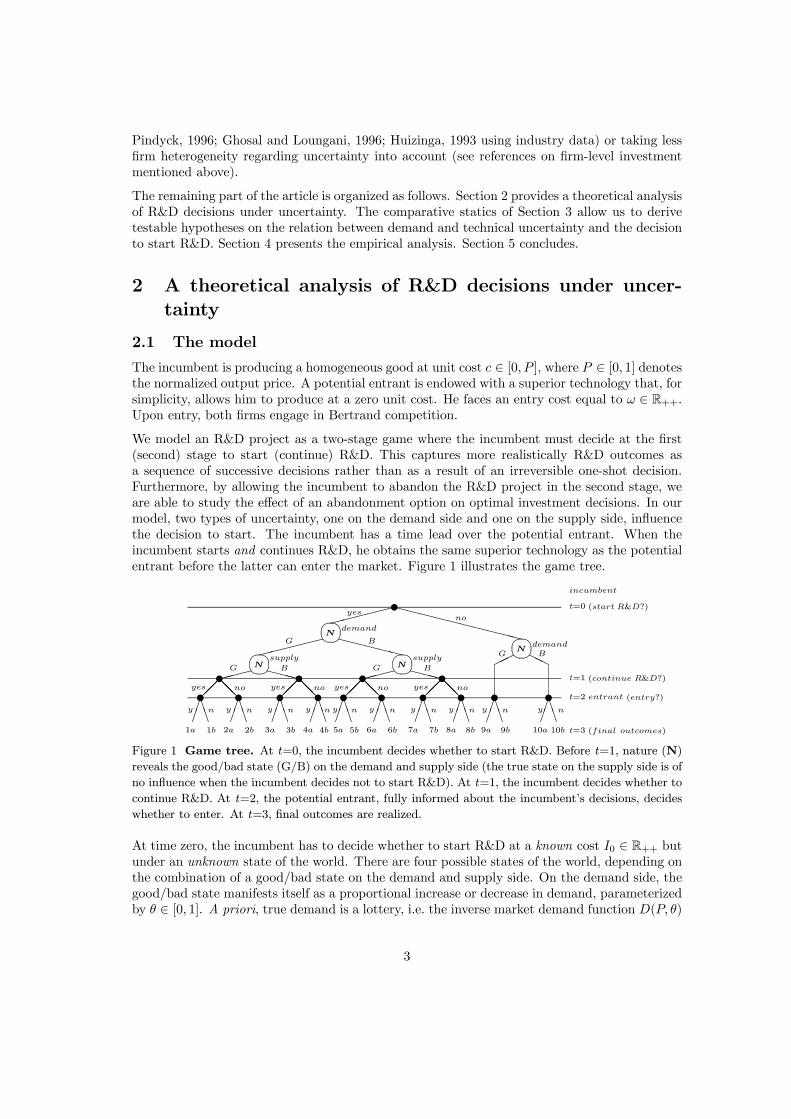
We model an R&D project as a two-stage game where the incumbent must decide at the first(second) stage to start (continue) R&D. This captures more realistically R&D outcomes asa sequence of successive decisions rather than as a result of an irreversible one-shot decision.Furthermore, by allowing the incumbent to abandon the R&D project in the second stage, weare able to study the effect of an abandonment option on optimal investment decisions. In ourmodel, two types of uncertainty, one on the demand side and one on the supply side, influencethe decision to start. The incumbent has a time lead over the potential entrant. When theincumbent starts and continues R&D, he obtains the same superior technology as the potentialentrant before the latter can enter the market. Figure 1 illustrates the game tree.

»»»»»XXXXXXXXXX»»»»»

XXXXX»»» XXX »»» XXX

¡¡@@ ¡¡@@ ¡¡@@ ¡¡@@

©© HH

¡¡ @@ ¡¡ @@ ¡¡ @@ ¡¡ @@££BB

££BB

££BB

££BB££BB

££BB

££BB

££BB

££BB

££BB

N

®­©ªsupply N

®­©ªsupplyN

®­©ªdemand

N

®­©ªdemand

G B G B

G B

G B

yesno

yes no yes no yes no yes no

y n y n y n y n y n y n y n y n y n y n

1a 1b 2a 2b 3a 3b 4a 4b 5a 5b 6a 6b 7a 7b 8a 8b 9a 9b 10a 10b

t

t t t tt t t t t t t t t t

incumbent

t=0 (start R&D?)

t=1 (continue R&D?)

t=2 entrant (entry?)

t=3 (final outcomes)

Figure 1 Game tree. At t=0, the incumbent decides whether to start R&D. Before t=1, nature (N)

reveals the good/bad state (G/B) on the demand and supply side (the true state on the supply side is of

no influence when the incumbent decides not to start R&D). At t=1, the incumbent decides whether to

continue R&D. At t=2, the potential entrant, fully informed about the incumbent’s decisions, decides

whether to enter. At t=3, final outcomes are realized.

At time zero, the incumbent has to decide whether to start R&D at a known cost I0 ∈ R++ butunder an unknown state of the world. There are four possible states of the world, depending onthe combination of a good/bad state on the demand and supply side. On the demand side, thegood/bad state manifests itself as a proportional increase or decrease in demand, parameterizedby θ ∈ [0, 1]. A priori, true demand is a lottery, i.e. the inverse market demand function D(P, θ)

3

equals (1 + θ) (1− P ) with probability pθ ∈ [0, 1] and (1− θ) (1− P ) with probability (1− pθ).On the supply side, the good/bad state manifests itself as a decrease or an increase in a knowncost I1 ∈ R++ to continue R&D, parameterized by λ ∈ [0, I1]. A priori, the true cost to continueR&D is a lottery, i.e. equal to (I1 − λ) with probability pλ ∈ [0, 1] and (I1 + λ) with probability(1− pλ). We assume that all parameters are known beforehand and that both lotteries areindependent. Before time one, nature (N) reveals the true state of the world.

At time one, the incumbent makes the decision whether to continue R&D.

At time two, the incumbent obtains the superior technology if he continued R&D. Having perfectknowledge about the incumbent’s decisions, the potential entrant makes his entry decision. Upona positive entry decision, the entrant enters the market, producing at a zero unit cost.

At time three, the final market structure is realized and the game ends.

2.2 Optimal entry decision and payoffs

The final market structure is never a duopoly.1 Indeed, if the incumbent does not possess thesuperior technology, the potential entrant can push the incumbent out of the market by settingthe price slightly under the incumbent’s unit production cost, i.e. P (c) = c − ε with ε > 0.However, entry is only optimal when monopoly profits are higher than or equal to the entrycost ω. If the potential entrant does not enter, the incumbent stays a monopolist who sets

P (c) = 1+c2 . The corresponding profits are π(c) =

(1−c)24 for all c ∈ [0, P ]. If the incumbent

does possess the superior technology, entry is never optimal. After all, the potential entrantknows that if he would enter, price equals marginal cost in equilibrium (P (0) = 0), and henceprofits equal zero (π(0) = 0), which do not cover the entry cost.

In order to characterize the optimal R&D decisions of the incumbent, we present the incumbent’spayoffs that correspond with the bottom row outcomes of Figure 1. We ignore the incumbent’smonopolistic profits at t = 0 and t = 1 since they are the same for any outcome of the gameand hence do not affect the incumbent’s investment decision.

Under scenarios 1, 3, 5 and 7, the incumbent possesses the superior technology and entry isnever optimal. Therefore, we only present the incumbent’s payoffs under b, which equal:

1b : (1 + θ)π(0)− I0 − (I1 − λ) 5b : (1− θ)π(0)− I0 − (I1 − λ)3b : (1 + θ)π(0)− I0 − (I1 + λ) 7b : (1− θ)π(0)− I0 − (I1 + λ)

Under scenarios 2, 4, 6, 8, 9 and 10, the incumbent does not possess the superior technology.Hence, entry can be optimal. Therefore, we present the incumbent’s payoffs valid under a (whenentry is optimal (π(0) ≥ ω)) and b (when entry is not optimal (π(0) < ω)).

2a : −I0 2b : (1 + θ)π(c)− I04a : −I0 4b : (1 + θ)π(c)− I06a : −I0 6b : (1− θ)π(c)− I08a : −I0 8b : (1− θ)π(c)− I09a : 0 9b : (1 + θ)π(c)10a : 0 10b : (1− θ)π(c)

1Since Bertrand competition results in a monopoly in our model, it is not meaningful to distinguish betweendrastic and non-drastic innovation (contrary to Cournot competition).

4

2.3 Optimal R&D decisions

We determine the optimal R&D decisions of the incumbent by backward induction. We startat t = 1. We denote the four possible states of the world by {GG,GB,BG,BB}, where thefirst character reflects the good (G) or bad (B) demand state and the second character reflectsthe good (G) or bad (B) supply state. Let the incumbent’s profit gain from innovation be∆π = π(0)− π(c). This profit gain is higher when the entrant enters the market than when theentrant does not enter the market, since π(c) = 0 for the incumbent in the former case, whereasπ(c) > 0 for the incumbent in the latter case. This immediately clarifies the strategic role ofthe entrant in our model compared to a monopoly model without entry threat. If the entry costis low enough to make entry optimal, the incumbent gets additional benefits from investing inthe superior technology. This strategic effect is known in the literature as Arrow’s replacementeffect (Arrow, 1962).

For each possible state of the world s ∈ {GG,GB,BG,BB}, we calculate ∆sNPV , i.e. the

difference between the net present value (NPV ) of continuing R&D and the NPV of notcontinuing R&D:

∆GGNPV = (1 + θ)∆π − (I1 − λ)

∆GBNPV = (1 + θ)∆π − (I1 + λ)

∆BGNPV = (1− θ)∆π − (I1 − λ)

∆BBNPV = (1− θ)∆π − (I1 + λ).

The incumbent continues R&D if and only if this difference is positive under the true state ofthe world, taking the entrant’s entry decision into account.

Optimal decision to continue r&d: For each possible state of the world s ∈ {GG,GB,BG,BB},the incumbent continues R&D if and only if ∆s

NPV ≥ 0.Let ψ = (ψGG, ψGB, ψBG, ψBB), where ψs = 1 when ∆

sNPV ≥ 0 and ψs = 0 when ∆

sNPV < 0

for all s ∈ {GG,GB,BG,BB}, be the vector that comprises the optimal decision to continueR&D under every possible state of the world. Notice that ∆GG

NPV ≥ ∆sNPV ≥ ∆BB

NPV for s ∈{GB,BG}. Thereforeψ ∈ Ψ = { (1, 1, 1, 1) , (1, 1, 1, 0) , (1, 1, 0, 0) , (1, 0, 1, 0) , (1, 0, 0, 0) , (0, 0, 0, 0) }.At t = 0, for every ψ ∈ Ψ, we calculate ∆ψNPV , i.e. the difference between the NPV of startingR&D and the NPV of not starting R&D. For every ψ ∈ Ψ, we determine the NPV of startingR&D by calculating the weighted sum of the incumbent’s payoffs when starting R&D in everypossible state of the world (using the probabilities of a good/bad state on the demand and supplyside as weights). We determine the NPV of not starting R&D by calculating the weighted sumof the incumbent’s payoffs when not starting R&D (using the probabilities of a good/bad stateon the demand and supply side as weights). The NPV of not starting R&D is the same forevery ψ ∈ Ψ.Hence, we get:

∆(1,1,1,1)NPV = pθpλ [(1 + θ)π(0)− I0 − (I1 − λ)]

+pθ (1− pλ) [(1 + θ)π(0)− I0 − (I1 + λ)]

+ (1− pθ) pλ [(1− θ)π(0)− I0 − (I1 − λ)]

+ (1− pθ) (1− pλ) [(1− θ)π(0)− I0 − (I1 + λ)]

− [pθ [(1 + θ)π(c)] + (1− pθ) [(1− θ)π(c)]]

= pθpλ∆GGNPV + pθ (1− pλ)∆

GBNPV + (1− pθ) pλ∆

BGNPV

+(1− pθ) (1− pλ)∆BBNPV − I0.

5

From this, we calculate:

∆(1,1,1,0)NPV = ∆

(1,1,1,1)NPV − (1− pθ) (1− pλ) [(1− θ)π(0)− I0 − (I1 + λ)]

+ (1− pθ) (1− pλ) [(1− θ)π(c)− I0]

= ∆(1,1,1,1)NPV − (1− pθ) (1− pλ)∆

BBNPV

= pθpλ∆GGNPV + pθ (1− pλ)∆

GBNPV + (1− pθ) pλ∆

BGNPV − I0.

Similarly, we get:

∆(1,1,0,0)NPV = pθpλ∆

GGNPV + pθ (1− pλ)∆

GBNPV − I0,

∆(1,0,1,0)NPV = pθpλ∆

GGNPV + (1− pθ) pλ∆

BGNPV − I0,

∆(1,0,0,0)NPV = pθpλ∆

GGNPV − I0,

∆(0,0,0,0)NPV = −I0.

Clearly, ∆(0,0,0,0)NPV < 0 and the incumbent does not start R&D.

The incumbent starts R&D if and only if there exists a positive ∆ψNPV for ψ ∈ Ψ\{ (0, 0, 0, 0) }.Note that these ∆ψNPV ’s cannot be ordered. For example, take ∆

(1,1,1,1)NPV and ∆

(1,1,1,0)NPV . We can

write ∆(1,1,1,1)NPV = ∆

(1,1,1,0)NPV + (1− pθ) (1− pλ)∆

BBNPV . If ∆

BBNPV > 0, then ∆

(1,1,1,1)NPV > ∆

(1,1,1,0)NPV

and it is possible to have ∆(1,1,1,1)NPV > 0, while ∆

(1,1,1,0)NPV < 0. On the other hand, if ∆BB

NPV < 0,

then ∆(1,1,1,1)NPV < ∆

(1,1,1,0)NPV and it is possible to have ∆

(1,1,1,1)NPV < 0, while ∆

(1,1,1,0)NPV > 0. A similar

argument can be made for any other comparison.

Therefore, let Φ = max{∆(1,1,1,1)NPV ,∆(1,1,1,0)NPV ,∆

(1,1,0,0)NPV ,∆

(1,0,1,0)NPV ,∆

(1,0,0,0)NPV }.

Optimal decision to start r&d: The incumbent starts R&D if and only if Φ ≥ 0.

3 Comparative statics

3.1 Relating divergence to uncertainty

In this section, we investigate how changes in demand and supply lotteries affect the incumbent’sdecision to start R&D. We therefore assume that entry is not optimal, because if entry wereoptimal, the entrant would drive the incumbent out of the market (cfr. Section 2.2). Throughoutthe remaining analysis, we use the following terminology. A lottery is defined to be favorable(unfavorable) if the probability of the good state is higher than or equal to (lower than) theprobability of the bad state. In comparing two lotteries, a lottery is defined to be more favorable(more unfavorable) than another lottery if the probability of the good state of the former is higher(lower) than the probability of the good state of the latter. However, we do not only distinguishbetween lotteries in terms of probabilities but also in terms of outcomes. In comparing twolotteries with equal probabilities, a lottery is defined to be more divergent (less divergent) thananother lottery if the difference between the good and the bad state is larger (smaller) in theformer than in the latter. In our model, the degree of divergence depends on θ and λ: a demand(supply) lottery becomes more divergent than another demand (supply) lottery when, ceterisparibus, θ (λ) increases and a demand (supply) lottery becomes less divergent than anotherdemand (supply) lottery when, ceteris paribus, θ (λ) decreases.

6

Let us first explain how a change in the degree of divergence of the demand (supply) lotteryrelates to a change in demand (technical) uncertainty. In this paper, we opt to quantify achange in uncertainty by a change in the risk premium. We define the risk premium of ademand (supply) lottery as the amount of money the incumbent is willing to pay (or has toreceive) to avoid undergoing the lottery. In our model, it equals the difference between obtainingdemand equal to 1 − P (facing the cost I1 of continuing R&D) and the expected outcome ofundergoing the demand (supply) lottery. One lottery is more uncertain than another lottery ifthe risk premium of the former is higher than the risk premium of the latter. It is clear that,when comparing a favorable lottery with an unfavorable lottery, the former is less uncertainthan the latter irrespective of the degree of divergence of both lotteries. After all, the riskpremium of a favorable lottery is negative whereas the risk premium of an unfavorable lotteryis strictly positive. Furthermore, favorable lotteries with probability 1

2 of the good/bad state(i.e. mean-preserving lotteries) are equally uncertain regardless of their degree of divergencesince their risk premium always equals 0. When comparing two favorable, non mean-preservinglotteries with equal probabilities, the more divergent lottery corresponds to the less uncertainlottery as the risk premium becomes more negative. Similarly, when comparing two unfavorablelotteries with equal probabilities, the more divergent lottery corresponds to the more uncertainlottery as the risk premium becomes more positive. However, we cannot always conclude thatthe more divergent lottery corresponds to the less (more) uncertain lottery when the lotteries arefavorable (unfavorable) but have unequal probabilities. Whether one lottery is more uncertainthan another lottery depends on the trade-off between (i) exactly how much more/less favorable(unfavorable) one lottery is compared to the other and (ii) how much less/more (more/less)divergent one lottery is compared to the other.

Having established the relationship between divergence and uncertainty, it remains to show howa change in the degree of divergence affects the decision to start R&D.

3.2 Relating divergence to the decision to start R&D

In Section 2, we derive that it is optimal for the incumbent to start R&D if and only if Φ ≥ 0.This decision depends on the vector of parameters (c, I0, I1, θ, pθ, λ, pλ). We now focus on howthe effect of an increase in θ on the decision to start R&D depends, ceteris paribus, on pθ. Acompletely similar reasoning, here omitted for reasons of parsimony, holds for how the effect ofan increase in λ depends, ceteris paribus, on pλ.

An increase from θ to θ0 can, ceteris paribus, either have one of the three effects on the decisionto start:

(i) a positive effect, i.e. when Φ(θ) < 0 and Φ(θ0) ≥ 0,(ii) a negative effect, i.e. when Φ(θ) ≥ 0 and Φ(θ0) < 0 or(iii) no effect, i.e. when Φ(θ) < 0 and Φ(θ0) < 0 or Φ(θ) ≥ 0 and Φ(θ0) ≥ 0.

Our approach aims at comparing Φ(θ) and Φ(θ0) for any θ, θ0 ∈ [0, 1] where θ < θ0. We want tomake explicit which effects are found for every pθ ∈ [0, 1], while restricting the parameter spaceof (c, I0, I1, λ, pλ) as little as possible.

Ceteris paribus, it is impossible to compare Φ(θ) and Φ(θ0) for any θ, θ0 ∈ [0, 1] where θ < θ0

and never find no effect, since Φ(θ) is a continuous function in θ.

Our first two propositions are straightforward. Proposition 1 states that a more divergentdemand lottery never positively affects the decision to start R&D when the demand lottery ismost unfavorable. After all, for a demand lottery that excludes the good state to happen, anincrease in θ corresponds to a worsening of the bad state, which never positively affects the

7

decision to start. Proposition 2 states that a more divergent demand lottery never negativelyaffects the decision to start R&D when the demand lottery belongs to the set of favorabledemand lotteries. After all, for demand lotteries where the good state is more likely to happenthan the bad state, an increase in θ a priori increases the attractiveness of the R&D projectand hence never affects the decision to start negatively. Both Propositions 1&2 hold over thecomplete parameter space of (c, I0, I1, λ, pλ). Remember that the same results are obtained byreplacing pθ and θ by pλ and λ respectively. All proofs are relegated to Appendix A.

Proposition 1: If pθ = 0, there does not exist a θ, θ0 ∈ [0, 1], where θ < θ0, such that Φ(θ) < 0and Φ(θ0) ≥ 0 for all (c, I0, I1, λ, pλ) ∈ [0, 1]×R3++ × [0, 1].Proposition 2: If pθ ∈ [12 , 1], there does not exist a θ, θ0 ∈ [0, 1], where θ < θ0, such thatΦ(θ) ≥ 0 and Φ(θ0) < 0 for all (c, I0, I1, λ, pλ) ∈ [0, 1]×R3++ × [0, 1].It remains to show how more divergent demand lotteries affect the decision to start R&D whenthe demand lottery is unfavorable. From Proposition 1, the open question is from which value ofpθ on, it is possible to find a positive effect. Similarly, from Proposition 2, the question remainsfrom which value of pθ on, it is not possible to find a negative effect. In other words, we aim atextending Propositions 1&2 by respectively finding the minimal values x ∈ (0, 1] and y ∈ [0, 12 ]such that the following results hold:

If pθ ∈ [0, x), there does not exist a θ, θ0 ∈ [0, 1], where θ < θ0, such that Φ(θ) < 0 andΦ(θ0) ≥ 0.If pθ ∈ [y, 1], there does not exist a θ, θ0 ∈ [0, 1], where θ < θ0, such that Φ(θ) ≥ 0 and

Φ(θ0) < 0.

The additional question becomes over which domains these extensions of Propositions 1&2 hold.Necessary conditions to obtain a positive (negative) effect are that, ceteris paribus, there existsa θ ∈ [0, 1] such that Φ(θ) ≥ (<)0. Obviously, these necessary conditions cannot be fulfilledover the complete parameter space of (c, I0, I1, λ, pλ). The intuition is that if the total costof undertaking the R&D project –which depends on (I0, I1, λ, pλ)– exceeds by far (is muchsmaller than) the total gain of the R&D project –which depends on (c, θ, pθ)–, then Φ willalways be negative (positive).

We impose two assumptions on the model, relating (in the absence of technical uncertainty) thecost of starting R&D to the cost of continuing R&D and the total cost of the R&D project tothe profit gain. We assume that (i) the two cost components of R&D would be the same in thetwo periods when λ = 0 and (ii) the total cost of R&D would equal the profit gain of R&D whenλ = 0.

Assumption 1: I0 = I1 = I.Assumption 2: I0 + I1 = ∆π.

Our results hold over the complete parameter space of (c, λ, pλ). Indeed, in relating differentdemand lotteries to the decision to start the R&D project, we deliberately do not want torestrict the set of lotteries on the supply side. In other words, in determining x and y, wechoose from the total set of supply lotteries (i) that particular lottery for which we obtain thesmallest interval pθ ∈ [0, x) of demand lotteries for which a more divergent demand lotterycannot positively affect the decision to start R&D and (ii) that particular lottery for which weobtain the smallest interval pθ ∈ [y, 1] of demand lotteries for which a more divergent demandlottery cannot negatively affect the decision to start R&D. Larger intervals than [0, x) and [y, 1]would be obtained if one excluded these particular supply lotteries from the total set. All resultsalso hold for any strictly positive value of c. When c equals zero, the incumbent never starts

8

the R&D project. A completely similar exercise is performed to relate changes in λ and valuesof pλ to changes in Φ under the complete parameter space of (c, θ, pθ).

2

Under Assumptions 1-2, we obtain Propositions 3a&3b for the minimal values x, v and Propo-sition 4 for the minimal values y, w respectively; all proofs are relegated to Appendix A:3

Proposition 3a: Under Assumptions 1-2, if pθ ∈ [0, 14), there does not exist a θ, θ0 ∈ [0, 1],where θ < θ0, such that Φ(θ) < 0 and Φ(θ0) ≥ 0 for all (c, λ, pλ) ∈ [0, 1]×R++ × [0, 1].Proposition 3b: Under Assumptions 1-2, if pλ ∈ [0, 0.28), there does not exist a λ, λ0 ∈ [0, 1],where λ < λ0, such that Φ(λ) < 0 and Φ(λ0) ≥ 0 for all (c, θ, pθ) ∈ [0, 1]3.Proposition 4: Under Assumptions 1-2, Proposition 2 is not extended: both y and w equal 12for all (c, λ, pλ) ∈ [0, 1]×R++ × [0, 1] and for all (c, θ, pθ) ∈ [0, 1]3 respectively.From Proposition 3a it follows that for the subset of unfavorable demand lotteries with pθ ∈[0, 14 ), a more divergent demand lottery never positively affects the decision to start R&D. Fromthe determination of y in Proposition 4 we learn that for all unfavorable demand lotteries, wecan not exclude that a more divergent demand lottery negatively affects the decision to startR&D. From Proposition 3b it follows that for the subset of unfavorable supply lotteries withpλ ∈ [0, 0.28), a more divergent supply lottery never positively affects the decision to start R&D.From the determination of w in Proposition 4 we learn that for all unfavorable supply lotteries,we cannot exclude that a more divergent supply lottery negatively affects the decision to startR&D.

Propositions 3a, 3b and 4 provide important additional insight in the relation between demand(supply) uncertainty and the decision to start R&D. Let us focus on demand uncertainty. Propo-sitions 3a and 4 demonstrate that, for the set of unfavorable demand lotteries with pθ ∈ [14 , 12)and depending inter alia on the supply lottery the incumbent faces, an increase in demanduncertainty can either positively or negatively affect the decision to start R&D. Especially thefact that an increase in demand uncertainty of an unfavorable demand lottery can positivelyaffect the decision to start R&D deserves some explanation. We obtain this result because of theabandonment option that the incumbent possesses. As we show in the proof of Proposition 3a

in Appendix A, an increase in θ positively affects the decision to start R&D when Φ = ∆(1,1,0,0)NPV .

Exactly in this case the R&D project is started under the assumption that the project will becompleted when the good state on the demand side occurs (although it is more likely that thebad state on the demand side occurs since the demand lottery is unfavorable). In other words,the incumbent completely ignores the downside risk of the R&D project when the bad state onthe demand side occurs exactly because it can abandon the project when this happens. Hence,

2More specifically, we aim at finding respectively the minimal values v ∈ (0, 1] and w ∈ [0, 12] such that the

following results hold:If pλ ∈ [0, v), there does not exist a λ, λ0 ∈ [0, 1], where λ < λ0, such thatΦ(λ) < 0 and Φ(λ0) ≥ 0 for all (c, θ, pθ) ∈ [0, 1]3.If pλ ∈ [w, 1], there does not exist a λ, λ0 ∈ [0, 1], where λ < λ0, such thatΦ(λ) ≥ 0 and Φ(λ0) < 0 for all (c, θ, pθ) ∈ [0, 1]3.3We performed a sensitivity analysis on Assumptions 1&2. We relax Assumption 1, setting I1 = aI0, where

a ∈ R++. We find that the higher (lower) the cost of continuing R&D compared to the cost of starting R&D, thesmaller (larger) the subset of unfavorable demand (supply) lotteries for which a more divergent demand (supply)lottery never positively affects the decision to start R&D. Furthermore, for all unfavorable demand/supplylotteries, we cannot exclude that a more divergent demand/supply lottery negatively affects the decision tostart R&D, whatever the relative importance of the two cost components I0 and I1. We relax Assumption 2by expressing the total cost of R&D as a proportion b ∈ R++ of the profit gain of R&D when λ = 0, i.e.I0 + I1 = b∆π. We find that the lower the profit gain of the R&D project compared to the total cost, the morefavorable the demand/supply lottery has to become in order to start R&D. For reasons of parsimony, we omitthe detailed results which are available upon request.

9

under the good state on the demand side, an increase in θ improves the profitability of the R&Dproject, which explains the result. If there were no abandonment option, an increase in demanduncertainty would never positively affect the decision to start R&D.4

4 An empirical analysis of the optimal decision to under-take R&D under uncertainty

4.1 Data

To test the propositions derived in the previous section, we use data from the 2005 officialinnovation survey in the German manufacturing and services industries which constitute theGerman part of the European-wide harmonized fourth Community Innovation Surveys (CISIV).5 The CIS data provide rich information on firms’ innovation behavior. The target popula-tion consists of all legally independent firms with at least 5 employees and their headquarterslocated in Germany.6 The survey is drawn as a stratified random sample and is representativeof the corresponding target population. The stratification criteria are firm size (8 size classesaccording to the number of employees), industry (22 two-digit industries according to the NACERev.1 classification system) and region (East and West Germany). The survey is performed bymail and in 2005 data on 4776 firms were collected (total sample), corresponding to a responserate of about 20%.7 In order to control for a response bias in the net sample, a non-responseanalysis was carried out collecting data on 4000 additional firms. A comparison shows that theinnovation behavior of respondents and non-respondents does not differ significantly. The shareof innovators is 63.9% in the former group and 62.2% in the latter group.8

For estimation purposes we exclude firms with incomplete data for any of the relevant variables(which are discussed in Section 4.2), ending up with a sample of 3681 firms. As illustrated inTable B.1 in Appendix B, our sample (full sample) reflects total-sample distributional charac-teristics very well and does not give any obvious cause for selectivity concerns. About 53.8% ofthe observed firms are in manufacturing.

4.2 Econometric model and testable hypotheses

Econometric model

In our theoretical model, the incumbent has to decide whether to undertake an R&D projectwhich aims at obtaining the same superior production technology as the potential entrant.9 Theoptimal decision to undertake R&D depends, ceteris paribus, on the degree of divergence of thedemand and supply lotteries. Empirically, we operationalize this optimal decision as follows.

4If the incumbent is forced to complete the R&D project once the project is started, he only will start the

project when ∆(1,1,1,1)NPV > 0. Note that

∂∆(1,1,1,1)NPV∂θ

= (2pθ − 1)∆π which is positive for all favorable demandlotteries and strictly negative for all unfavorable demand lotteries. This explains the result, given the relationbetween divergence and uncertainty (cfr. Section 3.1).

5The innovation surveys are conducted by the Centre for European Economic Research (ZEW), FraunhoferInstitute for Systems and Innovation Research (ISI) and infas Institute for Applied Social Sciences on behalf ofthe German Federal Ministry of Education and Research (BMBF). A detailed description of the data is given inPeters (2008).

6A firm is defined as the smallest combination of legal units operating as an organizational unit producinggoods or services.

7This rather low response rate is not unusual for surveys in Germany and is due to the fact that participationis voluntary.

8The p-value of the Fisher-test on equal shares in both groups amounts to 0.108.9In what follows, the notions firm and incumbent are used interchangeably.

10

Let y∗i denote firm i’s maximal difference between the NPV of undertaking R&D and the NPVof not undertaking R&D, which cannot be observed. Exploiting the firm heterogeneity in ourunique dataset, we assume that for firm i this difference depends on θi and λi, some otherobservable characteristics summarized in the row vector xi and unobservable factors capturedby i:

y∗i = αθi + γλi + xiβ + i (1)

In Section 2.3, we derive that it is optimal for incumbent i to undertake R&D if and only if y∗iis larger than or equal to zero:

yi =

½1 if y∗i ≥ 00 if y∗i < 0

(2)

where yi denotes the observed binary endogenous variable. We estimate equation (2) using theprobit estimator.

Testable hypotheses

Table 1 gives the descriptive statistics of all variables used in the econometric analysis andTable B.2 in Appendix B provides detailed definitions of all variables. We proxy the observedbinary endogenous variable (yi) by two variables. The first proxy indicates whether the firmhas performed R&D in the period 2002-2004 (R&D). Table 1 shows that 48% of the firms inthe full sample undertook R&D projects. However, over the same period, we observe θi andλi, our measures reflecting uncertainty on the demand and the supply side respectively. Due tothe short time-span of our data, we cannot use lagged values as instruments for the uncertaintymeasures to encounter the possible endogeneity problem. Instead, we employ as an alternativeproxy an expected decision, indicating whether the firm plans to introduce a new productiontechnology in the next year 2005 (PROCESS). We find that 46% of the firms in the full sampleplanned to introduce a process innovation.

<Insert Table 1 about here>

In our theoretical model, demand uncertainty stems from the two components in the lottery onthe demand side: the degree of divergence (represented by θ) and the probability (pθ) of facinga good demand state. The variable θ is measured by the average of the absolute percentagechange in sales over the last two years 2002-2003 and 2003-2004 (THETA).10 Table 1 revealsthat the absolute change in sales was on average about 14 % in the last two years. In ourbenchmark estimations, we assume that pθ is the same for all firms. Our dataset enables us torelax this assumption later on.

Similarly, technical uncertainty is represented by the two components in the lottery on the sup-ply side: the degree of divergence (parameterized by λ) and the probability (pλ) of facing a goodsupply state. For the full sample, λ can only be proxied by a dummy variable LAMBDA1.LAMBDA1 equals 1 if an innovation project was extended due to high innovation costs in theperiod 2002-2004. The motivation for using this information is that an unexpected delay of aninnovation project is presumably associated with unexpected higher costs. Hence, LAMBDA1partitions the set of firms into a subset of firms with a low degree of divergence and a subsetof firms with a high degree of divergence. Around 19% of the firms belong to the latter. Alter-natively, we use a second proxy for λ (LAMBDA2) which is defined as the absolute deviationbetween on the one hand the R&D expenditures for 2004 expected in 2003 and on the otherhand the realized R&D expenditures in 2004. The virtue of this measure is that it more closelycorresponds to the way we model λ in our theoretical analysis. The defect is that we can apply

10We implicitly assume that firms expect sales to stay constant over the short time-span under consideration.

11

it only to a subset of enterprises since we have to use the prior wave of the innovation survey toconstruct this variable.11 However, this subsample is representative for the full sample as canbe inferred from Table B.1 in Appendix B. The average absolute deviation between expectedand realized innovation expenditure comes to 2.4 mill. Euro. The deviation turns out to behighly skewed. We therefore use a logarithmic transformation of this variable in the econometricanalysis. In all our estimations, we assume that pλ is the same for all firms. Our dataset doesnot allow to relax this assumption.

The probabilities pθ and pλ are determined as follows. To calculate pθ using the full sample, wederive that 56.9% of the firms experienced a positive growth in sales between 2002 and 2003 and61.8% between 2003 and 2004. No information is available to calculate pλ from the full sample.However, we are able to determine pλ from the subsample. More specifically, we observe that for59.4% of the firms, realized innovation expenditure in 2004 turns out to be lower than expectedin 2003. Given the representativeness of the subsample, we assume that the calculated pλ isalso valid for the full sample.

Assuming that pθ and pλ are the same for all firms and given that pθ and pλ are calculated tobe larger than 1

2 , we postulate from Proposition 2 the following hypotheses.

Hypothesis 1: The probability of undertaking R&D does not decrease with a more divergentdemand lottery.

Hypothesis 2: The probability of undertaking R&D does not decrease with a more divergentsupply lottery.

In our theoretical model, the incumbent is challenged by a potential competitor. Our datareveal that about 91% of the firms perceive a threat of its own market position due to thepotential entry of new competitors. In the estimations, we therefore control for potential entryby including 3 dummy variables indicating whether the firm perceives a high, medium or lowthreat.

We also control for the following factors found to be important in the literature. Two maindeterminants explaining innovation activities go back to Schumpeter (1942), who states thatlarge firms in concentrated markets have an advantage in innovation. Therefore, we include firmsize (SIZE) and market structure (NUMCOMP ). Firm size is measured by the logarithm ofthe number of employees in 2003 and we expect a positive relationship. Market structure iscaptured by 3 dummy variables indicating the number of competitors. Schumpeter stresses anegative relationship between competition and innovation. His argument is that ex ante productmarket power on the one hand increases monopoly rents from innovation and on the other handreduces the uncertainty associated with excessive rivalry. Recently, Aghion et al. (2005) findevidence for an inverted U -relationship between competition and innovation. For low initiallevels of competition an escape-competition effect dominates (i.e. competition increases theincremental profits from innovating, and, thereby, encourages innovation investments) whereasthe Schumpeterian effect tends to dominate at higher levels of competition.

The incentive to engage in R&D may further depend on the type of competition (COMP ).We include 5 dummy variables indicating whether firms primarily compete in prices, productquality, technological lead, product variety or product design.

The innovation literature stresses that certain firm characteristics –such as the degree of prod-uct diversification, the degree of internationalization, the availability of financial resources and

11In Germany, the innovation surveys are conducted annually and they are designed as a panel (so calledMannheim Innovation Panel). Unfortunately, the overlap between the 2004 and 2005 survey only amounts toalmost 40% due to a major refreshment and enlargement of the gross sample.

12

technological capabilities– are likewise crucial for explaining innovation (see, e.g., the refer-ences cited in Peters, 2008). More diversified firms possess economies of scope in innovation.As they have more opportunities to exploit new knowledge and complementarities among theirdiversified activities, they tend to be more innovative. We measure product diversification bythe share of turnover of the firm’s most important product in 2004 (DIV ERS). Therefore, weexpect a negative coefficient since more diversified firms exhibit lower values for this proxy.

The more a firm is exposed to international competition, the more likely the firm engages inR&D activities. The degree to which a firm is exposed to international competition is capturedby a dummy variable taking the value of 1 if the firm sells its products to international markets(EXPORT ).

The availability of financial resources is proxied by an index of creditworthiness (RATING). Alower creditworthiness implies less available and more costly external funding to finance R&Dprojects. Since the index ranges from 1 (best rating) to 6 (worst rating), we expect a negativecoefficient for this proxy.

Innovative capabilities are determined by the skills of employees. We take into account theshare of employees with a university degree (HIGHSKILLED), a dummy variable being 1 ifthe firm has not invested in training its employees (NOTRAIN) and the amount of trainingexpenditure per employee (TRAINEXP ) if the firm has invested in training. Since informationon training expenditure is missing for 11.3% of the firms, we do not drop these observations butrather set the expenditure to zero and include a dummy variable indicating the missing valuestatus (MV TRAIN).

We also include variables reflecting whether the firm is located in East Germany (EAST ) andwhether the firm is part of an enterprise group (GROUP ). A priori, the effect of these variablesis unclear. Finally, industry dummies are included in all regressions.

4.3 Results

4.3.1 Firms facing equal lottery probabilities

Table 2 reports the marginal effects of the probit estimates for the full sample, assuming that allfirms face the same probabilities in the demand and supply lotteries. For each of the two endoge-nous variables, the first column reports the results for a parsimonious specification –includingonly SIZE and industry dummies in addition to demand uncertainty, technical uncertainty andentry threat– whereas the second column employs the full set of control variables described inthe previous section.

<Insert Table 2 about here>

Hypothesis 1, postulating that the probability of undertaking R&D does not decrease with anincrease in θ, is strongly confirmed. Focusing on our preferred specification (R&D (2)), ourresults indicate that a 10% increase in θ increases the likelihood of undertaking R&D by 1.4%.

Hypothesis 2, postulating that the probability of undertaking R&D does not decrease with anincrease in λ, is strongly confirmed. This result is robust across the two endogenous variablesand holds when additional control variables are incorporated. We estimate that a change froma low to a high degree of divergence increases the likelihood of undertaking R&D by 23.3%.

Entry threat does not significantly influence the decision to undertake R&D. As R&D andTHREAT are measured over the same period, an endogeneity problem might arise as the

13

decision to perform R&D could reduce the perceived entry threat. This explanation is supportedby the fact that entry threat does significantly positively affect the decision to undertake processinnovations in the next year.

Regarding the impact of the other control variables, most results are in line with expectations.Firm size exerts a significantly positive impact. Market structure has a non-linear effect oninnovation. Firms in oligopoly markets have a higher likelihood of undertaking R&D or in-troducing new products compared to monopolists or firms with more competitors. Hence, ourresults support evidence in favor of the inverted U -relationship between competition and inno-vation as suggested by Aghion et al. (2005). Another striking and robust finding is that firmsacting on markets where competition is mainly settled through prices are less likely to innovate.On the contrary, innovation activities are stimulated if competitive advantage can be achievedby technological leadership. Firms being exposed to international competition as well as morediversified firms have a higher likelihood of undertaking R&D and introducing new products.There is, however, no significant impact on process innovation. Finally, the results highlight theimportant role of innovative capabilities. Firms employing a higher share of high-skilled workersor firms investing in training are likely to be more innovative.

For the subsample, Table 3 presents in columns (2) and (4) the estimates using our preferredmeasure for technical uncertainty (LAMBDA2). For reasons of comparison, columns (1) and(3) show the subsample results employing LAMBDA1. In general, the results are very similarto the full sample. Hypothesis 2 is also strongly confirmed using LAMBDA2. Since we measurethis variable in logarithm, a value of 0.017 implies that an increase in the deviation of expectedand actual R&D expenditure by 10% increases the propensity to undertake R&D by 17%.12

<Insert Table 3 about here>

4.3.2 Firms facing different demand lottery probabilities

In this section we relax the assumption that the probability of facing a good demand state isthe same for all firms. We approximate pθ by looking at the firms’ sales histories in the pasttwo years. We define three groups of firms (see Table B.2 in Appendix B for exact definitions).Group 1 (G1) comprises all firms that experienced a decrease in sales in 2002-2003 as well asin 2003-2004. The idea is that these firms face an unfavorable demand lottery reflected by alow value of pθ. These firms are much more likely to face a bad demand state than a gooddemand state. Group 2 (G2) consists of all firms that experienced one yearly decrease and oneyearly increase in sales during the period 2002-2004. On the basis of this observation, we assumethat these firms face equal probabilities of a good/bad demand state and therefore have a pθaround 1

2 . All firms in group 3 (G3) experienced an increase in sales in 2002-2003 as well as in2003-2004. The assumption is that these firms face a favorable demand lottery reflected by ahigh value of pθ.

Assuming that firms in group 1 have a pθ smaller than14 , firms in group 2 have a pθ around

12

and firms in group 3 have a pθ larger than12 , we postulate from Proposition 3a and Proposition

2 respectively the following hypotheses.

Hypothesis 3: For firms in group 1, the probability of undertaking R&D does not increasewith a more divergent demand lottery.

12To test whether multicollinearity between our main independent variables affect our results in Tables 2 and 3,we estimate specifications that include demand uncertainty, technical uncertainty or entry threat separately andspecifications that combine demand uncertainty or technical uncertainty with entry threat. The significance aswell as the magnitude of the estimated marginal effects are very robust in both the full sample and the subsample(results available upon request).

14

Hypothesis 4: For firms in group 2 and group 3, the probability of undertaking R&D does notdecrease with a more divergent demand lottery.

Table 4 presents the results of distinguishing the effect of a more divergent demand lottery acrossgroups of firms facing different demand lottery probabilities. Confirming hypothesis 3, we findthat for firms in group 1 the effect of an increase in θ is significantly negative for PROCESSand negative but not significant for R&D in the specifications including all control variables.Furthermore, the impact of THETA is significantly different for firms in group 1 compared tofirms in group 2 and group 3. Hypothesis 4 is strongly confirmed since the impact of THETAis never significantly negative for firms in group 2 and group 3. Moreover, in all specifications,the effect of a more divergent demand lottery is significantly positive for firms in group 3.Furthermore, the impact is significantly larger for firms in group 3 than for firms in group 2when process innovations are considered.13

<Insert Table 4 about here>

5 Conclusion

This article contributes to the theoretical as well as the empirical literature on R&D decisionsunder uncertainty.

From a theoretical point of view, we study a two-stage R&D project with an abandonmentoption. Two types of uncertainty influence the decision to start R&D. Demand uncertaintyis modelled as a lottery between a proportional increase and decrease in demand. Technicaluncertainty is modelled as a lottery between a decrease and increase in the cost to continueR&D. Both lotteries become more divergent when the difference between the outcomes of thelottery increases. We relate differences in uncertainty to differences in risk premia. This allowsus to consider a broader set of demand and supply lotteries than only the subset of lotteries thatpreserve the mean, as previously studied in the literature. A potential entrant is endowed witha superior technology and threatens to drive the incumbent out of the market. The incumbenthas a time lead over the entrant and can obtain the same superior technology by completing theR&D project before the entrant can enter the market. The presence of the entrant in our modelprovides the incumbent with additional benefits from investing in the superior technology, astrategic effect known as Arrow’s replacement effect. In order to deduct testable hypotheses, wederive under which lottery probabilities more divergent demand and supply lotteries positivelyor negatively affect the decision to start R&D. Under mild assumptions, relating (in the absenceof technical uncertainty) the cost of starting R&D to the cost of continuing R&D and the totalcost of the R&D project to the profit gain, our most counterintuitive result is that an increasein the degree of divergence of an unfavorable demand lottery can positively affect the decisionto start R&D. We obtain this result because of the abandonment option that the incumbentpossesses.

From an empirical point of view, we test the hypotheses derived from the theoretical modelusing data from the fourth Community Innovation Survey (CIS IV) data in Germany. Theuniqueness of our data lies in the availability of proxies for demand and technical uncertaintyas well as perceived entry threat for about 4000 firms to explain actual and planned R&Dinvestments. Our main results, strongly confirming our model predictions, are that for firmsfacing lotteries where the good state is more likely to prevail (i) a 10% increase in the degree of

13To test the robustness of the results in Table 4, we make a distinction between manufacturing and services.Hypotheses 2, 3 and 4 are confirmed in both samples (results available upon request).

15

divergence of the demand lottery increases the likelihood of undertaking R&D by 1.4% and (ii)a change from a low to a high degree of divergence of the supply lottery increases the likelihoodof undertaking R&D by 23.3%. Using a subsample of firms for which we have a proxy forthe degree of divergence of the supply lottery that more closely corresponds to our theoreticalmodel, gives similar estimation results. For firms facing a demand lottery where the bad stateis more likely to prevail, an increase in the degree of divergence of the demand lottery decreasesthe probability of undertaking R&D significantly.

References

[1] Aghion, P., N. Bloom, R. Blundell, R. Griffith and P. Howitt, 2005, Competition andinnovation: An inverted U -relationship, Quarterly Journal of Economics, 120(2), 701-728.

[2] Arrow, K., 1962, The economic implications of learning by doing, Review of EconomicStudies, 29(3), 155-173.

[3] Bloom, N., S. Bond and J. Van Reenen, 2007, Uncertainty and investment dynamics,Review of Economic Studies, 74(2), 391-415.

[4] Caballero, R. and R.S. Pindyck, 1996, Investment, uncertainty and industry evolution,International Economic Review, 37(3), 641-662.

[5] Darby, J., A.H. Hallett, J. Ireland and L. Piscitelli, 1999, The impact of exchange rateuncertainty on the level of investment, Economic Journal, 109(454), c55-c67.

[6] Dasgupta, P. and J. Stiglitz, 1980, Industrial structure and the nature of innovative activity,Economic Journal, 90(4), 266-293.

[7] Dixit, A. and R.S. Pindyck, 1994, Investment under uncertainty, Princeton, New Jersey:Princeton University Press.

[8] Dorfman, J.H. and D. Heien, 1989, The effects of uncertainty and adjustment costs oninvestment in the almond industry, The Review of Economics and Statistics, 71(2), 263-274.

[9] Eiser R. and M.I. Nadiri, 1968, Investment behavior and Neo-Classical theory, The Reviewof Economics and Statistics, 50(3), 369-382.

[10] Farzin, Y., K. Huisman and P. Kort, 1998, Optimal timing of technology adoption, Journalof Economic Dynamics and Control, 22(5), 779-799.

[11] Ferderer, J.P., 1993, The impact of uncertainty on aggregate investment spending: Anempirical analysis, Journal of Money, Credit, and Banking, 25(1), 30-48.

[12] Ghosal, V. and P. Loungani, 1996, Product market competition and the impact of priceuncertainty on investment: Some evidence from US manufacturing industries, Journal ofIndustrial Economics, 44(2), 217-228.

[13] Grenadier, S., 2000, Game choices: The intersection of real options and game theory,London: Risk Books.

[14] Grenadier, S. and A. Weiss, 1997, Investment in technological innovations: An optionpricing approach, Journal of Financial Economics, 44(3), 397-416.

16

[15] Guiso, L. and G. Parigi, 1999, Investment and demand uncertainty, Quarterly Journal ofEconomics, 114(1), 185-227.

[16] Henley, A., A. Carruth and A. Dickerson, 2003, Industry-wide versus firm-specific uncer-tainty and investment: British company panel data evidence, Economics Letters, 78(1),87-92.

[17] Huizinga, J., 1993, Inflation uncertainty, relative price uncertainty, and investment in U.S.manufacturing, Journal of Money, Credit, and Banking, 25(3), 521-557.

[18] Jorgenson, D.W., 1963, Capital theory and investment behavior, American Economic Re-view, 53(2), 247-259.

[19] Leahy, J. and T. Whited, 1996, The effect of uncertainty on investment: Some stylizedfacts, Journal of Money, Credit and Banking, 28(1), 64-83.

[20] Lukach, R., P.M. Kort and J. Plasmans, 2007, Optimal R&D investment strategies underthe threat of new technology entry, International Journal of Industrial Organization, 25(1),103-119.

[21] Peters, B., 2008, Innovation and firm performance. An empirical investigation for Germanfirms, ZEW Economic Studies, 38, Heidelberg, New York.

[22] Pindyck, R.S., 1993, Investments of uncertain cost, Journal of Financial Economics, 34(1),53-76.

[23] Pratt, J., 1964, Risk aversion in the small and in the large, Econometrica, 32(1-2), 122-136.

[24] Tyagi, R., 2006, New product introductions and failures under uncertainty, InternationalJournal of Research in Marketing, 23(2), 199-213.

[25] Weeds, H., 2002, Strategic delay in a real options model of R&D competition, Review ofEconomic Studies, 69(3), 729-747.

17

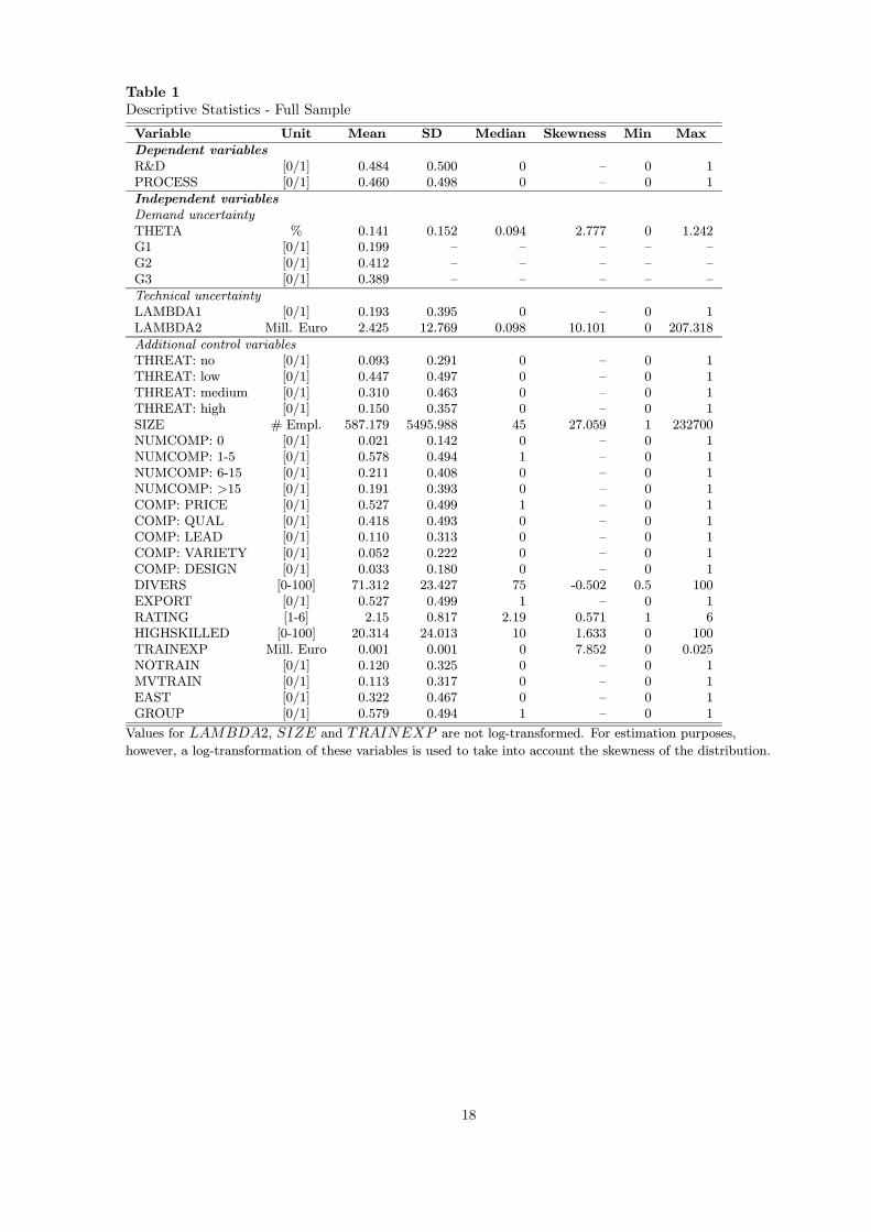
Table 1Descriptive Statistics - Full Sample

Variable Unit Mean SD Median Skewness Min Max

Dependent variablesR&D [0/1] 0.484 0.500 0 — 0 1PROCESS [0/1] 0.460 0.498 0 — 0 1

Independent variablesDemand uncertaintyTHETA % 0.141 0.152 0.094 2.777 0 1.242G1 [0/1] 0.199 — — — — —G2 [0/1] 0.412 — — — — —G3 [0/1] 0.389 — — — — —

Technical uncertaintyLAMBDA1 [0/1] 0.193 0.395 0 — 0 1LAMBDA2 Mill. Euro 2.425 12.769 0.098 10.101 0 207.318

Additional control variablesTHREAT: no [0/1] 0.093 0.291 0 — 0 1THREAT: low [0/1] 0.447 0.497 0 — 0 1THREAT: medium [0/1] 0.310 0.463 0 — 0 1THREAT: high [0/1] 0.150 0.357 0 — 0 1SIZE # Empl. 587.179 5495.988 45 27.059 1 232700NUMCOMP: 0 [0/1] 0.021 0.142 0 — 0 1NUMCOMP: 1-5 [0/1] 0.578 0.494 1 — 0 1NUMCOMP: 6-15 [0/1] 0.211 0.408 0 — 0 1NUMCOMP: >15 [0/1] 0.191 0.393 0 — 0 1COMP: PRICE [0/1] 0.527 0.499 1 — 0 1COMP: QUAL [0/1] 0.418 0.493 0 — 0 1COMP: LEAD [0/1] 0.110 0.313 0 — 0 1COMP: VARIETY [0/1] 0.052 0.222 0 — 0 1COMP: DESIGN [0/1] 0.033 0.180 0 — 0 1DIVERS [0-100] 71.312 23.427 75 -0.502 0.5 100EXPORT [0/1] 0.527 0.499 1 — 0 1RATING [1-6] 2.15 0.817 2.19 0.571 1 6HIGHSKILLED [0-100] 20.314 24.013 10 1.633 0 100TRAINEXP Mill. Euro 0.001 0.001 0 7.852 0 0.025NOTRAIN [0/1] 0.120 0.325 0 — 0 1MVTRAIN [0/1] 0.113 0.317 0 — 0 1EAST [0/1] 0.322 0.467 0 — 0 1GROUP [0/1] 0.579 0.494 1 — 0 1

Values for LAMBDA2, SIZE and TRAINEXP are not log-transformed. For estimation purposes,

however, a log-transformation of these variables is used to take into account the skewness of the distribution.

18

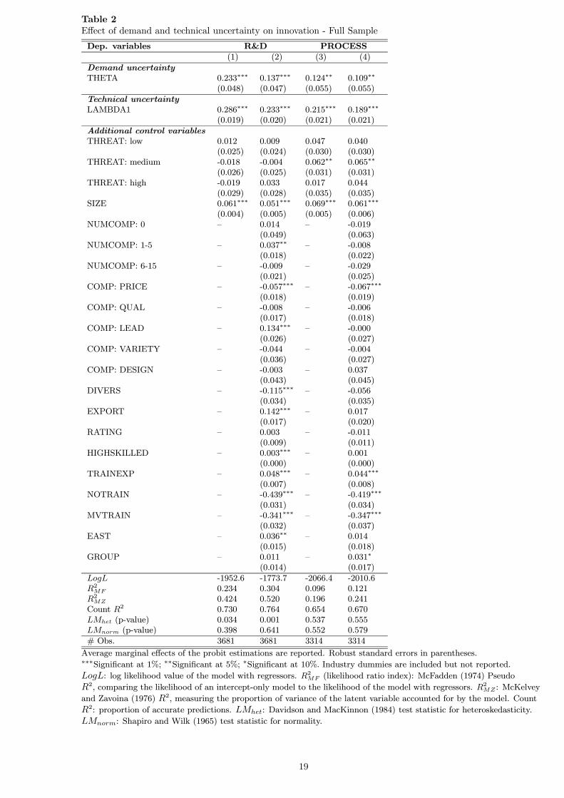
Table 2Effect of demand and technical uncertainty on innovation - Full Sample

Dep. variables R&D PROCESS

(1) (2) (3) (4)

Demand uncertaintyTHETA 0.233∗∗∗ 0.137∗∗∗ 0.124∗∗ 0.109∗∗

(0.048) (0.047) (0.055) (0.055)

Technical uncertaintyLAMBDA1 0.286∗∗∗ 0.233∗∗∗ 0.215∗∗∗ 0.189∗∗∗

(0.019) (0.020) (0.021) (0.021)

Additional control variablesTHREAT: low 0.012 0.009 0.047 0.040

(0.025) (0.024) (0.030) (0.030)THREAT: medium -0.018 -0.004 0.062∗∗ 0.065∗∗

(0.026) (0.025) (0.031) (0.031)THREAT: high -0.019 0.033 0.017 0.044

(0.029) (0.028) (0.035) (0.035)SIZE 0.061∗∗∗ 0.051∗∗∗ 0.069∗∗∗ 0.061∗∗∗

(0.004) (0.005) (0.005) (0.006)NUMCOMP: 0 — 0.014 — -0.019

(0.049) (0.063)NUMCOMP: 1-5 — 0.037∗∗ — -0.008

(0.018) (0.022)NUMCOMP: 6-15 — -0.009 — -0.029

(0.021) (0.025)COMP: PRICE — -0.057∗∗∗ — -0.067∗∗∗

(0.018) (0.019)COMP: QUAL — -0.008 — -0.006

(0.017) (0.018)COMP: LEAD — 0.134∗∗∗ — -0.000

(0.026) (0.027)COMP: VARIETY — -0.044 — -0.004

(0.036) (0.027)COMP: DESIGN — -0.003 — 0.037

(0.043) (0.045)DIVERS — -0.115∗∗∗ — -0.056

(0.034) (0.035)EXPORT — 0.142∗∗∗ — 0.017

(0.017) (0.020)RATING — 0.003 — -0.011

(0.009) (0.011)HIGHSKILLED — 0.003∗∗∗ — 0.001

(0.000) (0.000)TRAINEXP — 0.048∗∗∗ — 0.044∗∗∗

(0.007) (0.008)NOTRAIN — -0.439∗∗∗ — -0.419∗∗∗

(0.031) (0.034)MVTRAIN — -0.341∗∗∗ — -0.347∗∗∗

(0.032) (0.037)EAST — 0.036∗∗ — 0.014

(0.015) (0.018)GROUP — 0.011 — 0.031∗

(0.014) (0.017)

LogL -1952.6 -1773.7 -2066.4 -2010.6R2MF 0.234 0.304 0.096 0.121

R2MZ 0.424 0.520 0.196 0.241

Count R2 0.730 0.764 0.654 0.670LMhet (p-value) 0.034 0.001 0.537 0.555LMnorm (p-value) 0.398 0.641 0.552 0.579

# Obs. 3681 3681 3314 3314

Average marginal effects of the probit estimations are reported. Robust standard errors in parentheses.∗∗∗Significant at 1%; ∗∗Significant at 5%; ∗Significant at 10%. Industry dummies are included but not reported.LogL: log likelihood value of the model with regressors. R2

MF (likelihood ratio index): McFadden (1974) Pseudo

R2, comparing the likelihood of an intercept-only model to the likelihood of the model with regressors. R2MZ : McKelvey

and Zavoina (1976) R2, measuring the proportion of variance of the latent variable accounted for by the model. Count

R2: proportion of accurate predictions. LMhet: Davidson and MacKinnon (1984) test statistic for heteroskedasticity.

LMnorm: Shapiro and Wilk (1965) test statistic for normality.

19

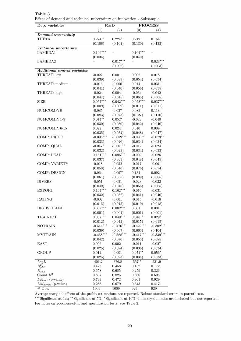
Table 3Effect of demand and technical uncertainty on innovation - Subsample

Dep. variables R&D PROCESS

(1) (2) (3) (4)

Demand uncertaintyTHETA 0.274∗∗ 0.224∗∗ 0.219∗ 0.154

(0.106) (0.101) (0.130) (0.122)

Technical uncertaintyLAMBDA1 0.196∗∗∗ — 0.161∗∗∗ —

(0.034) (0.040)LAMBDA2 — 0.017∗∗∗ — 0.023∗∗∗

(0.002) (0.003)

Additional control variablesTHREAT: low -0.022 0.001 0.002 0.018

(0.039) (0.039) (0.054) (0.054)THREAT: medium -0.016 -0.000 0.014 0.031

(0.041) (0.040) (0.056) (0.055)THREAT: high -0.024 0.004 -0.064 -0.042

(0.047) (0.045) (0.065) (0.065)SIZE 0.057∗∗∗ 0.042∗∗∗ 0.058∗∗∗ 0.037∗∗∗

(0.009) (0.009) (0.011) (0.011)NUMCOMP: 0 -0.085 -0.037 0.083 0.118

(0.083) (0.073) (0.127) (0.110)NUMCOMP: 1-5 0.074∗∗ 0.052∗ -0.023 -0.040

(0.030) (0.030) (0.042) (0.040)NUMCOMP: 6-15 0.022 0.024 0.010 0.009

(0.035) (0.034) (0.048) (0.047)COMP: PRICE -0.098∗∗∗ -0.089∗∗∗ -0.090∗∗ -0.079∗∗

(0.033) (0.026) (0.034) (0.034)COMP: QUAL -0.047∗ -0.061∗∗∗ -0.012 -0.024

(0.032) (0.023) (0.034) (0.033)COMP: LEAD 0.131∗∗∗ 0.096∗∗∗ -0.002 -0.026

(0.037) (0.033) (0.048) (0.045)COMP: VARIETY -0.018 -0.052 -0.017 -0.061

(0.058) (0.046) (0.076) (0.074)COMP: DESIGN -0.064 -0.097∗ 0.134 0.092

(0.061) (0.055) (0.089) (0.085)DIVERS -0.051 -0.051 -0.023 -0.022

(0.049) (0.046) (0.066) (0.065)EXPORT 0.164∗∗∗ 0.162∗∗∗ -0.016 -0.031

(0.032) (0.032) (0.041) (0.040)RATING -0.002 -0.001 -0.015 -0.016

(0.015) (0.015) (0.019) (0.018)HIGHSKILLED 0.002∗∗∗ 0.002∗∗∗ 0.001 0.001

(0.001) (0.001) (0.001) (0.001)TRAINEXP 0.067∗∗∗ 0.049∗∗∗ 0.048∗∗∗ 0.029∗

(0.012) (0.012) (0.015) (0.015)NOTRAIN -0.544∗∗∗ -0.476∗∗∗ -0.422∗∗∗ -0.302∗∗∗

(0.039) (0.067) (0.063) (0.104)MVTRAIN -0.458∗∗∗ -0.388∗∗∗ -0.417∗∗∗ -0.339∗∗∗

(0.042) (0.070) (0.053) (0.085)EAST 0.006 0.002 -0.011 -0.027

(0.025) (0.024) (0.036) (0.034)GROUP 0.014 -0.001 0.071∗∗ 0.056∗

(0.025) (0.023) (0.034) (0.033)

LogL -401.2 -376.8 -557.5 -531.9R2MF 0.423 0.458 0.132 0.172

R2MZ 0.658 0.685 0.259 0.326

Count R2 0.807 0.825 0.666 0.695LMhet (p-value) 0.733 0.472 0.961 0.929LMnorm (p-value) 0.288 0.679 0.343 0.417

# Obs. 1009 1009 929 929

Average marginal effects of the probit estimations are reported. Robust standard errors in parentheses.∗∗∗Significant at 1%; ∗∗Significant at 5%; ∗Significant at 10%. Industry dummies are included but not reported.For notes on goodness-of-fit and specification tests: see Table 2.

20

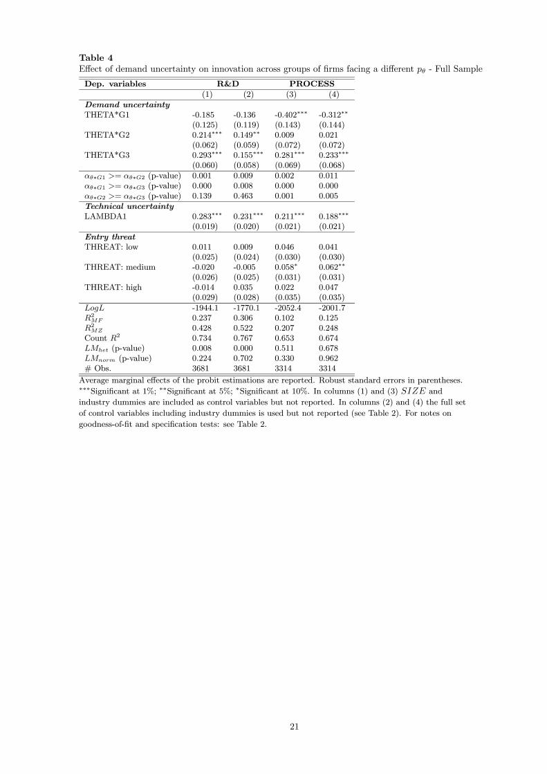
Table 4Effect of demand uncertainty on innovation across groups of firms facing a different pθ - Full Sample

Dep. variables R&D PROCESS

(1) (2) (3) (4)

Demand uncertaintyTHETA*G1 -0.185 -0.136 -0.402∗∗∗ -0.312∗∗

(0.125) (0.119) (0.143) (0.144)THETA*G2 0.214∗∗∗ 0.149∗∗ 0.009 0.021

(0.062) (0.059) (0.072) (0.072)THETA*G3 0.293∗∗∗ 0.155∗∗∗ 0.281∗∗∗ 0.233∗∗∗

(0.060) (0.058) (0.069) (0.068)

αθ∗G1 >= αθ∗G2 (p-value) 0.001 0.009 0.002 0.011αθ∗G1 >= αθ∗G3 (p-value) 0.000 0.008 0.000 0.000αθ∗G2 >= αθ∗G3 (p-value) 0.139 0.463 0.001 0.005

Technical uncertaintyLAMBDA1 0.283∗∗∗ 0.231∗∗∗ 0.211∗∗∗ 0.188∗∗∗

(0.019) (0.020) (0.021) (0.021)

Entry threatTHREAT: low 0.011 0.009 0.046 0.041

(0.025) (0.024) (0.030) (0.030)THREAT: medium -0.020 -0.005 0.058∗ 0.062∗∗

(0.026) (0.025) (0.031) (0.031)THREAT: high -0.014 0.035 0.022 0.047

(0.029) (0.028) (0.035) (0.035)

LogL -1944.1 -1770.1 -2052.4 -2001.7R2MF 0.237 0.306 0.102 0.125

R2MZ 0.428 0.522 0.207 0.248

Count R2 0.734 0.767 0.653 0.674LMhet (p-value) 0.008 0.000 0.511 0.678LMnorm (p-value) 0.224 0.702 0.330 0.962# Obs. 3681 3681 3314 3314

Average marginal effects of the probit estimations are reported. Robust standard errors in parentheses.∗∗∗Significant at 1%; ∗∗Significant at 5%; ∗Significant at 10%. In columns (1) and (3) SIZE and

industry dummies are included as control variables but not reported. In columns (2) and (4) the full set

of control variables including industry dummies is used but not reported (see Table 2). For notes on

goodness-of-fit and specification tests: see Table 2.

21

Appendix A: Proofs

Proof of Propositions 1 & 2: Consider the partial derivatives of the five arguments of Φ with

respect to θ:∂∆

(1,1,1,1)NPV

∂θ = (2pθ − 1)∆π, ∂∆(1,1,1,0)NPV

∂θ = (pθ − pλ + pθpλ)∆π,∂∆

(1,1,0,0)NPV

∂θ = pθ∆π,∂∆

(1,0,1,0)NPV

∂θ = pλ (2pθ − 1)∆π, ∂∆(1,0,0,0)NPV

∂θ = pθpλ∆π. All five partial derivatives are either negativeor equal to zero when pθ = 0 for all pλ ∈ [0, 1]. This is a sufficient condition to obtain Proposition1. All five partial derivatives are either positive or equal to zero when pθ ∈ [12 , 1] for all pλ ∈ [0, 1].This is a sufficient condition to obtain Proposition 2. ¥

Proofs of Propositions 3a, 3b & 4: Before we prove Propositions 3a, 3b & 4 consequently, weintroduce Lemma 1 and Lemma 1’. Lemma 1 identifies Φ for different ranges of the parametersθ and λ. Lemma 1 holds over the complete parameter space of (c, pθ, pλ).

Lemma 1:(1) Φ = ∆

(1,1,1,1)NPV for all θ ∈ [0, 12 ] and for all λ ∈ [0,

¡12 − θ

¢∆π].

(2) Φ = ∆(1,1,1,0)NPV for all θ ∈ [0, 12 ] and for all λ ∈ [

¡12 − θ

¢∆π, λmax].

(3) Φ = ∆(1,1,0,0)NPV for all θ ∈ [ 12 , 1] and for all λ ∈ [0,

¡θ − 1

2

¢∆π].

(4) Φ = ∆(1,1,1,0)NPV for all θ ∈ [ 12 , 1] and for all λ ∈ [

¡θ − 1

2

¢∆π, λmax].

Proof of Lemma 1: From Assumptions 1-2, it follows that λmax = I = ∆π2 . Then, ∆

GBNPV ≥ 0

when¡12 + θ

¢∆π ≥ λ. Therefore, ∆GB

NPV ≥ 0 for all θ ∈ [0, 1] and λ ∈ [0, λmax]. As a result,also ∆GG

NPV ≥ 0 for all θ ∈ [0, 1] and λ ∈ [0, λmax] (cfr. Section 2.3). Then, ∆BGNPV ≥ 0 when¡

θ − 12

¢∆π ≤ λ. Therefore, ∆BG

NPV ≥ 0 for all θ ∈ [0, 12 ] and for all λ ∈ [0, λmax], ∆BGNPV ≤ 0

for all θ ∈ [12 , 1] and for all λ ∈ [0,¡θ − 1

2

¢∆π] and ∆BG

NPV ≥ 0 for all θ ∈ [12 , 1] and for allλ ∈ [¡θ − 1

2

¢∆π], λmax]. Then, ∆

BBNPV ≥ 0 when

¡12 − θ

¢∆π ≥ λ. Therefore, ∆BB

NPV ≥ 0

for all θ ∈ [0, 12 ] and for all λ ∈ [0,¡12 − θ

¢∆π], ∆BB

NPV ≤ 0 for all θ ∈ [0, 12 ] and for all

λ ∈ [¡12 − θ¢∆π, λmax] and ∆

BBNPV ≤ 0 for all θ ∈ [12 , 1] and for all λ ∈ [0, λmax]. Lemma 1

follows from noting that Φ = ∆(1,1,1,1)NPV when ∆GB

NPV ≥ 0, ∆BGNPV ≥ 0 and ∆BB

NPV ≥ 0, that

Φ = ∆(1,1,1,0)NPV when ∆GB

NPV ≥ 0, ∆BGNPV ≥ 0 and ∆BB

NPV ≤ 0 and that Φ = ∆(1,1,1,0)NPV when

∆GBNPV ≥ 0, ∆BG

NPV ≤ 0 and ∆BBNPV ≤ 0. ¥

We use Lemma 1, where λ is expressed as a function of θ, in the determination of x and y. Forthe determination of v and w, it is useful to rewrite Lemma 1 as Lemma 1’ where we express θas a function of λ. Again, Lemma 1’ holds over the complete parameter space of (c, pθ, pλ).

Lemma 1’:(1) Φ = ∆

(1,1,1,1)NPV for all λ ∈ [0, λmax] and for all θ ∈ [0, λmax−λ∆π ].

(2) Φ = ∆(1,1,1,0)NPV for all λ ∈ [0, λmax] and for all θ ∈ [λmax−λ∆π , λmax+λ∆π ].

(3) Φ = ∆(1,1,0,0)NPV for all λ ∈ [0, λmax] and for all θ ∈ [λmax+λ∆π , 1].

Proof of Proposition 3a: We prove that the smallest pθ for which a positive effect of anincrease in θ on the decision to start R&D is found, equals 1

4 by showing that Φ(θ) = 0 for

Φ = ∆(1,1,0,0)NPV , θ = 1, pθ =

14 , λ = λmax and pλ = 1.

First, consider the partial derivatives of ∆(1,1,1,1)NPV , ∆

(1,1,1,0)NPV and ∆

(1,1,0,0)NPV with respect to θ when

pθ ∈ [0, 12 ]. Note that∂∆

(1,1,1,1)NPV

∂θ = (2pθ − 1)∆π ≤ 0, ∂∆(1,1,1,0)NPV

∂θ = (pθ − pλ + pθpλ)∆π ≥ 0 if

22

and only if pλ ≤ pθ1−pθ and

∂∆(1,1,0,0)NPV

∂θ = pθ∆π ≥ 0. A positive effect due to an increase in θ can

only be found when ∂Φ(θ)∂θ ≥ 0 at some subdomain of θ.

Second, from the fact that ∆GGNPV ≥ ∆s

NPV ≥ ∆BBNPV for s ∈ {GB,BG} (cfr. Section 2.3), it

follows that∂∆

(1,1,1,1)NPV

∂pθ= pλ

¡∆GGNPV −∆BG

NPV

¢+ (1− pλ) (∆

GBNPV − ∆BB

NPV ) ≥ 0,∂∆

(1,1,1,0)NPV

∂pθ=

pλ¡∆GGNPV −∆BG

NPV

¢+ (1− pλ)∆

GBNPV ≥ 0 and

∂∆(1,1,0,0)NPV

∂pθ= pλ∆

GGNPV + (1− pλ)∆

GBNPV ≥ 0.

From these observations and the definition of x, it follows that when pθ = x, Φ(θ) = 0 whenθ = 1.

Third, from Lemma 1, Φ(1) = 0 holds for Φ = ∆(1,1,0,0)NPV . Solving ∆

(1,1,0,0)NPV (1) = 0 yields

pθ =12∆π

32∆π+(2pλ−1)λ

. We find x by solving minλ,pλ

pθ. For λ = λmax and pλ = 1, x =14 . ¥

Proof of Proposition 3b: We prove that the smallest pλ for which a positive effect of anincrease in λ on the decision to start R&D is found, approximately equals 0.28 by showing that

Φ(λ) = 0 for Φ = ∆(1,1,1,0)NPV , λ = λmax, pλ = 0.28, θ = 1, and pθ =

pλ1−pλ .

First, consider the partial derivatives of ∆(1,1,1,1)NPV , ∆

(1,1,1,0)NPV and ∆

(1,1,0,0)NPV with respect to λ when

pλ ∈ [0, 12 ]. Note that∂∆

(1,1,1,1)NPV

∂λ = (2pλ − 1)∆π ≤ 0, ∂∆(1,1,1,0)NPV

∂λ = (−pθ + pλ + pθpλ)∆π ≥ 0 ifand only if pθ ≤ pλ

1−pλ and∂∆

(1,1,0,0)NPV

∂λ = pθ(2pλ − 1)∆π ≤ 0 for all pθ ∈ [0, 1]. A positive effectdue to an increase in λ can only be found when ∂Φ(λ)

∂λ ≥ 0 at some subdomain of λ.Second,

∂∆(1,1,1,1)NPV

∂pλ= pθ

¡∆GGNPV −∆GB

NPV

¢+ (1− pθ)

¡∆BGNPV −∆BB

NPV

¢ ≥ 0 and∂∆

(1,1,0,0)NPV

∂pλ=

pθ¡∆GGNPV −∆GB

NPV

¢ ≥ 0. Also, ∂∆(1,1,1,0)NPV

∂pλ= pθ

¡∆GGNPV −∆GB

NPV

¢+ (1− pθ)∆

BGNPV ≥ 0 if and

only if ∆BGNPV ≥ 0. This is the case when Φ = ∆

(1,1,1,0)NPV . From these observations and the

definition of v, it follows that when pλ = v, Φ(λ) = 0 when λ = λmax.

Third, from Lemma 1’, Φ(λmax) = 0 holds for Φ = ∆(1,1,1,0)NPV when θ ∈ [0, 1]. Solving

∆(1,1,1,0)NPV (λmax) = 0 yields pλ =

12−pθθ

1−θ+pθθ . We find v by solving minθ,pθ

pλ subject to pθ ≤ pλ1−pλ .

For θ = 1 and pθ =pλ1−pλ , v = 0.280776 ≈ 0.28. ¥

Proof of Proposition 4: We first prove that the lowest pθ for which no negative effect of anincrease in θ on the decision to start R&D can be found, equals 12 by showing that Φ(θ) = 0 for

Φ = ∆(1,1,1,0)NPV , θ = 1

2 , pθ =12 , λ = 0 and pλ = 1.

First, a negative effect due to an increase in θ can only be found when ∂Φ(θ)∂θ ≤ 0 at some

subdomain of θ. Hence, Φ has to be equal to ∆(1,1,1,1)NPV or ∆

(1,1,1,0)NPV when pλ ≥ pθ

1−pθ at somesubdomain of θ.

Second, from the observation that∂∆

(1,1,1,1)NPV

∂pθ≥ 0,∂∆

(1,1,1,0)NPV

∂pθ≥ 0 and ∂∆

(1,1,0,0)NPV

∂pθ≥ 0 (cfr. proof

of Proposition 3a) and from the definition of y, two possibilities arise. Either, Φ(θ) = 0 for

θ = 12 and pθ = y, when (i) for θ ∈ [0, 12 ], Φ = ∆

(1,1,1,1)NPV or Φ = ∆

(1,1,1,0)NPV and pλ ≥ pθ

1−pθand for θ ∈ [12 , 1], Φ = ∆(1,1,0,0)NPV or when (ii) for θ ∈ [0, 12 ], Φ = ∆(1,1,1,1)NPV and for θ ∈ [12 , 1],Φ = ∆

(1,1,0,0)NPV or Φ = ∆

(1,1,1,0)NPV and pλ ≤ pθ

1−pθ . Or Φ(θ) = 0 for θ = 1 and pθ = y when, for

θ ∈ [0, 12 ], Φ = ∆(1,1,1,1)NPV or Φ = ∆(1,1,1,0)NPV and pλ ≥ pθ

1−pθ and for θ ∈ [12 , 1], Φ = ∆(1,1,1,0)NPV and

pλ ≥ pθ1−pθ .

23

Third, from Lemma 1, Φ( 12) = 0 holds for Φ = ∆(1,1,1,0)NPV for all λ ∈ [0, λmax] when pλ ≥ pθ

1−pθ .

Solving ∆(1,1,1,0)NPV (12) = 0 yields pθ =

12∆π−pλλ∆π−(1−pλ)λ . We find y by solving max

λ,pλpθ subject to

pλ ≥ pθ1−pθ . For λ = 0 and pλ = 1, y = 1

2 . Since y cannot exceed12 (cfr. Proposition 2), the

result follows.

We now prove that the lowest pλ for which no negative effect of an increase in λ on the decision

to start R&D can be found, equals 12 by showing that Φ(λ) = 0 for Φ = ∆

(1,1,1,0)NPV , λ = λmax,

pλ =12 , θ = 0 and pθ = 1.

First, a negative effect due to an increase in λ can only be found when ∂Φ(λ)∂λ ≤ 0 at some

subdomain of λ. Hence, in order to find a negative effect, Φ has to be equal to ∆(1,1,1,1)NPV ,

∆(1,1,0,0)NPV or ∆

(1,1,1,0)NPV when p

θ≥ pλ

1−pλ at some subdomain of λ.

Second, from the observation that∂∆

(1,1,1,1)NPV

∂pλ≥ 0,∂∆

(1,1,1,0)NPV

∂pλ≥ 0 and ∂∆

(1,1,0,0)NPV

∂pλ≥ 0 (cfr. proof

of Proposition 3b) and from the definition of w, it follows that when pλ = w, Φ(λ) = 0 whenλ = λmax.

Third, from Lemma 1’, Φ(λmax) = 0 holds for Φ = ∆(1,1,1,0)NPV for all θ ∈ [0, 1] when p

θ≥ pλ

1−pλ .

Solving ∆(1,1,1,0)NPV (λmax) = 0 yields pλ =

12−pθθ

1−θ+pθθ . We find w by solving maxθ,pθ

pλ subject to

pθ≥ pλ

1−pλ . For θ = 0 and pθ = 1, w =12 . Since w cannot exceed

12 , the result follows. ¥

24

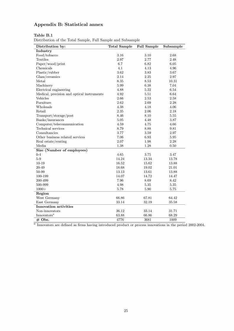
Appendix B: Statistical annex

Table B.1Distribution of the Total Sample, Full Sample and Subsample

Distribution by: Total Sample Full Sample Subsample

IndustryFood/tobacco 3.16 3.10 2.68Textiles 2.97 2.77 2.48Paper/wood/print 6.7 6.82 6.05Chemicals 4.1 4.13 4.96Plastic/rubber 3.62 3.83 3.67Glass/ceramics 2.14 2.25 2.97Metal 8.35 8.53 10.31Machinery 5.99 6.38 7.04Electrical engineering 4.88 5.22 6.54Medical, precision and optical instruments 4.92 5.51 6.64Vehicles 2.66 2.53 2.58Furniture 2.62 2.69 2.28Wholesale 4.38 4.18 4.06Retail 2.35 2.06 2.18Transport/storage/post 8.46 8.10 5.55Banks/insurances 5.05 4.48 3.87Computer/telecommunication 4.59 4.75 4.66Technical services 8.79 8.88 9.81Consultancies 3.77 3.59 2.97Other business related services 7.06 6.93 5.95Real estate/renting 2.07 1.98 2.28Media 1.38 1.28 0.50

Size (Number of employees)0-4 4.65 3.75 3.475-9 14.24 13.34 13.7810-19 16.52 15.62 13.8820-49 18.68 19.02 21.0150-99 13.13 13.61 13.88100-199 14.07 14.72 14.47200-499 7.96 8.69 8.42500-999 4.98 5.35 5.351000+ 5.78 5.90 5.75

RegionWest Germany 66.86 67.81 64.42East Germany 33.14 32.19 35.58

Innovation activitiesNon-innovators 36.12 33.14 31.71Innovatorsa 63.88 66.86 68.29

# Obs. 4776 3681 1009a Innovators are defined as firms having introduced product or process innovations in the period 2002-2004.

25

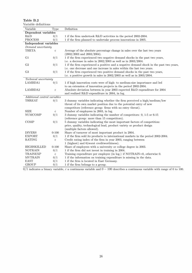
Table B.2Variable definitions

Variable Type Definition

Dependent variablesR&D 0/1 1 if the firm undertook R&D activities in the period 2002-2004.PROCESS 0/1 1 if the firm planned to undertake process innovations in 2005.

Independent variablesDemand uncertaintyTHETA c Average of the absolute percentage change in sales over the last two years

(2002/2003 and 2003/2004).G1 0/1 1 if the firm experienced two negative demand shocks in the past two years,

i.e. a decrease in sales in 2002/2003 as well as in 2003/2004.G2 0/1 1 if the firm experienced a positive and a negative demand shock in the past two years,

i.e. one decrease and one increase in sales within the last two years.G3 0/1 1 if the firm experienced two positive demand shocks in the past two years,

i.e. a positive growth in sales in 2002/2003 as well as in 2003/2004.

Technical uncertaintyLAMBDA1 0/1 1 if high innovation costs were of high- to medium-size importance and led

to an extension of innovation projects in the period 2002-2004.LAMBDA2 c Absolute deviation between in year 2003 expected R&D expenditure for 2004

and realized R&D expenditure in 2004, in log.

Additional control variablesTHREAT 0/1 3 dummy variables indicating whether the firm perceived a high/medium/low

threat of its own market position due to the potential entry of newcompetitors (reference group: firms with no entry threat).

SIZE c Number of employees in 2003, in log.NUMCOMP 0/1 3 dummy variables indicating the number of competitors: 0, 1-5 or 6-15

(reference group: more than 15 competitors).COMP 0/1 5 dummy variables indicating the most important factors of competition:

price, quality, technological lead, product variety or product design(multiple factors allowed).

DIVERS 0-100 Share of turnover of most important product in 2004.EXPORT 0/1 1 if the firm sold its products to international markets in the period 2002-2004.RATING c Credit rating index of the firm in year 2003, ranging between

1 (highest) and 6(worst creditworthiness).HIGHSKILLED 0-100 Share of employees with a university or college degree in 2003.NOTRAIN 0/1 1 if the firm did not invest in training in 2004.TRAINEXP c Training expenditure per employee (in log.) if NOTRAIN=0, otherwise 0.MVTRAIN 0/1 1 if the information on training expenditure is missing in the data.EAST 0/1 1 if the firm is located in East Germany.GROUP 0/1 1 if the firm belongs to a group.

0/1 indicates a binary variable, c a continuous variable and 0− 100 describes a continuous variable with range of 0 to 100.

26