Embed Size (px)
Citation preview
DEPARTMENT OF ECONOMICS
MODEL UNCERTAINTY AND BAYESIAN MODEL
AVERAGING IN VECTOR AUTOREGRESSIVE
PROCESSES
Rodney W. Strachan, University of Leicester, UK
Herman K. van Dijk, Erasmus University, The Netherlands
Working Paper No. 06/5 February 2006

Model Uncertainty and Bayesian ModelAveraging in Vector Autoregressive Processes
Rodney W. Strachan1�
Herman K. van Dijk21Department of Economics, University of Leicester,
Leicester LE1 7RH UK.email: [email protected]
2Econometric Institute,Erasmus University Rotterdam,Rotterdam, The Netherlands
email: [email protected]
February 6, 2006
�Corresponding author.
1

ABSTRACT
Economic forecasts and policy decisions are often informed by empiri-cal analysis based on econometric models. However, inference based upona single model, when several viable models exist, limits its usefulness. Tak-ing account of model uncertainty, a Bayesian model averaging procedure ispresented which allows for unconditional inference within the class of vectorautoregressive (VAR) processes. Several features of VAR process are investi-gated. Measures on manifolds are employed in order to elicit uniform priorson subspaces de�ned by particular structural features of VARs. The featuresconsidered are the number and form of the equilibrium economic relationsand deterministic processes. Posterior probabilities of these features are usedin a model averaging approach for forecasting and impulse response analysis.The methods are applied to investigate stability of the �Great Ratios� inU.S. consumption, investment and income, and the presence and e¤ects ofpermanent shocks in these series. The results obtained indicate the feasibilityof the proposed method.
Key Words:Posterior probability; Grassman manifold; Orthogonal group;Cointegration; Model averaging; Stochastic trend; Impulse response;Vector autoregressive model.
JEL Codes: C11, C32, C52
2

1 Introduction.
In this paper we take account of model uncertainty and introduce a method ofusing Bayesian model averaging in the class of vector autoregressive processes.We demonstrate the operational implications of our approach by investigat-ing the stability of the �Great Ratios�in U.S. consumption, investment andincome, and analysing the presence and e¤ects of permanent shocks for theduration of the business cycle in these series.The idea underlying Bayesian model averaging is relatively straightfor-
ward. Model speci�c estimates are weighted by the corresponding posteriormodel probability and then averaged over the set of models considered. Al-though many statistical arguments have been made in the literature to sup-port model averaging (e.g., Leamer, 1978, Hodges, 1987, Draper, 1995, Minand Zellner, 1993 and Raftery, Madigan and Hoeting, 1997), recent applica-tions suggest its relevance for macroeconometrics (Fernández, Ley and Steel,2001 and Sala-i-Martin, Doppelho¤er and Miller, 2004). Here we mentionthree reasons for this relevance.The �rst reason is relevance for forecasting and policy analysis. An im-
portant function of empirical economic analysis is to provide accurate infor-mation for decision making. For example, there is evidence that permanent -possibly productivity - shocks account for most �uctuations in consumption(King, Plosser, Stock and Watson, 1991, and Lettau and Ludvigson, 2004)and information may be required on the form of the response in consumptionto such a permanent shock. Centoni and Cubadda (2003), however, focusupon business cycle �uctuations and �nd permanent shocks are not very im-portant. While the decision maker is not directly interested in the underlyingmodel used to estimate the response, it is, however, the econometrician�s re-sponsibility to detail the model upon which these estimates rely. If thereis any uncertainty about the veracity of the model, the expected loss (fromchoosing a policy action) from that single model cannot equal the expectedloss that accurately accounts for model uncertainty.A second reason for considering model averaging is methodological. There
are well known issues relating to the complexity of the model set and thesequences used to select a model. The standard approach to providing in-ference is to select a single model and present empirical results based uponthis model. The usual strategy of model selection using sequential testingprocedures, however, introduces problems of model uncertainty. In the con-text of sequential hypothesis testing, the pre-test problem is well understood
3

(see, for example, Poirier, 1995, pp. 519-523) and has received considerableattention in the statistical and econometric literature. We do not intend (norare able) to survey the literature here, but mention that just within the unitroot and cointegration testing there have been several studies such as Elliottand Stock (1994), Elliott (1998), Phillips (1996), Chang and Phillips (1995)and Chang (2000) (see for useful discussion, Maddala and Kim, 1998, pp.139-140 and 229-231).The problem is self evident. Whether we accept or do not accept an
hypothesis, the veracity of the adopted hypothesis is uncertain. Subsequenttests condition upon that uncertain outcome and have their own uncertainoutcomes. This process can lead to signi�cant size distortions and inappro-priate reported standard errors. Generally, the resulting standard errors willnot fully re�ect the uncertainty associated with the estimates. The longerthe sequence of tests the more the problem compounds, and the sequencecan become very long if, for example, we consider: lag length; the type ofdeterministic processes present; the number of cointegrating relations; overi-dentifying restrictions on the cointegrating space; and even whether certainvariables are in some sense (weakly or strongly) exogenous for the inferencein question. Despite the extensive concern shown in the literature for thepretest problem, however, a generally applicable strategy for dealing withthis issue does not appear to be available. It would seem the usual (implicit)approach is to �. . . entirely ignore the problems caused by pretesting, notbecause they are unimportant, but because, in practice, they are generallyintractable�(Davidson and MacKinnon, 1993, pp. 97-98).An additional, related, problem due to the complexity of the model, is
the con�icting inferences that may arise depending upon which sequence oftests is employed. For example, using the Johansen trace test and data onconsumption, investment and income from Paap and van Dijk (2003), we�nd that the chosen cointegrating rank depends upon the chosen determin-istic term1 and the rank may be zero or one. This suggests it is importantto determine the correct deterministic process before investigating the coin-tegrating rank. However, the range of deterministic process that can occurdi¤ers if cointegration occurs or not. To take this example further, let usassume a rank of one for these variables and we are now interested in 1)
1As the deterministic processes enter the error correction term, testing for presence of atrend in a VAR in levels, when cointegration is present, does not identify the deterministicprocess.
4

whether the error correction term, zt; has a trend and 2) if the Great Ratiosof consumption to income and investment to income enter zt.2 Dependingupon whether we test stability of the Great Ratios �rst or test the presenceof various deterministic terms �rst, we �nd either we have no trend in zt andthat the Great Ratios do not enter zt; or that the Great Ratios do enter ztand zt has a linear trend.A third reason for considering Bayesian model averaging is a pragmatic
one. The support in the data is in many cases not clear or dogmatically foror against a restriction, and researchers often do not have strong prior beliefin particular restrictions. The strategy of testing hypotheses on restrictionsand conditioning upon the outcome, e¤ectively assigns a weight of one to themodel implied by the restriction and zero to all other plausible models. Evenif the support is strongly for or against a particular restriction, with onlyslight support for the alternative unrestricted model, imposing the restric-tion ignores information from that less likely model which, if appropriatelyweighted, could improve inference.Thus, there is a con�ict between the analyst�s need to obtain the best
model and the decision-maker�s need for the least restrictive interpretationof the information provided by the analyst. As an alternative to conditioningon structural features, it is possible to improve policy analysis by present-ing unconditional or averaged information. Gains in forecasting accuracy bysimple averaging have been pioneered by Bates and Granger (1969) and dis-cussed recently by Diebold and Lopez (1996), Newbold and Harvey (2001)and Terui and van Dijk (2002). Some explanation for this phenomenon inparticular cases was provided by Hendry and Clements (2002). Alternatively,the averaging weights can be determined to re�ect the support for the modelfrom which each estimate derives. This requires accurate re�ection of theuncertainty associated with the structural features de�ning the model.We present a Bayesian approach for conducting unconditional inference
from the vector autoregressive model. Speci�cally, we focus on three con-tributions. First, a general operational procedure is presented for specify-ing di¤use prior information on structural features of interest which implieswell-de�ned posteriors and existence of moments. Given the prior, the infor-mation in the likelihood function is supposed to dominate. As a result onecan evaluate the relative weights or probabilities of such structural featuresas the number of stable equilibrium relationships among economic variables,
2This implies a particular overidentifying restriction on the cointegrating space holds.
5

the forms of those equilibrium relationships, the dynamic responses to dis-equilibria, and the type of deterministic processes that may be present. Inorder to obtain these results we make of use manifolds and orthogonal groupsand their measures. Then we can elicit uniform prior measures on relevantsubspaces of the parameter space. From these measures we develop priordistributions for elements of these subspaces as the parameter of interest.Second, using this methodology we show in this paper how to obtain pos-
terior inference and forecasts from model averages in which the economicallyand econometrically important structural features may have weights otherthan zero or one.Third, we brie�y demonstrate the proposed methodology with an inves-
tigation of the stability of the �Great Ratios�as discussed in King, Plosser,Stock and Watson (1991) (hereafter KPSW), and the relative weights ofpermanent and transitory components in US consumption, investment andincome, and, �nally, the credibility of alternative paths of responses to apossible productivity shock.There exist several Bayesian analyses of VAR processes in the literature.
A complete survey is outside the scope of our paper, although we mentionthe following approaches. Using so-called �Minnesota�priors, which are of arandom walk nature, Doan, Litterman and Sims (1984) investigate Bayesianforecasting and impulse response analysis using unrestricted VARs. Simsand Zha (1999) investigate con�dence bands of impulse responses using un-restricted VARs. Other papers using unrestricted VARs include Koop (1991and 1994) and Canova and Matteo (2004). Structural features in VAR mod-els, like cointegration, are investigated by Kleibergen and Van Dijk (1994),Strachan (2003), Villani (2005) using di¤use type of priors. We extend theanalysis of these two approaches by considering priors on structural fea-tures and by investigating the implied forecasts and impulse responses usingBayesian model averaging.The structure of the paper is as follows. In the Section 2 we introduce
the models of interest in this paper - the vector autoregressive models, thegeneral structural features of interest, and the restrictions they imply. InSection 3 we present the priors, the likelihood and useful expressions for theposterior. The tools for inference in this paper, posterior probabilities, areintroduced and general expressions are derived for estimators of features ofinterest like impulse responses. Our approach is a signi�cant divergence frommuch of the earlier work. This section therefore provides a discussion of theadvantages of this approach in the context of model averaging. We demon-
6

strate the approach in Section 4 with an investigation of the responses ofconsumption, investment and income to a permanent shock allowing for sta-bility of consumption to income and investment to income ratios. In Section5 we summarize conclusions and discuss possibilities for further research.
2 A Set of Vector Autoregressive Models.
Since the in�uential work by Sims (1980), the vector autoregressive model hasenjoyed much success in macroeconometrics. These models can incorporatea wide range of short and long run dynamic, equilibrium and deterministicbehaviours. Further, it has been observed in empirical studies, that manyeconomic variables of interest are not stationary, yet economic theory, orempirical evidence, suggests stable long run relationships to exist amongthese variables.The statistical theory of cointegration (Granger, 1983, and Engle and
Granger, 1987), in which a set of nonstationary variables combine linearlyto form stationary relationships, and the attendant Granger�s representationtheorem provide a useful speci�cation to incorporate this economic behaviourinto the error correction model and allows the separation of long run and shortrun behaviour. We work with the vector autoregressive model in the errorcorrection form to simplify expressions of restrictions. For more details on alikelihood analysis of VAR models with cointegration restrictions we refer toJohansen (1995).When a VAR process cointegrates, the model may be written in the vector
error correction model (VECM) form. The VECM of the 1� n vector timeseries process yt; t = 1; : : : ; T; conditioning on the l observations t = �l +1; : : : ; 0; is
�yt =�d1;t�1 + yt�1�
+��+ d2;t�2 +�yt�1�1 + : : :+�yt�l�l + "t (1)
= z1;t�� + z2;t� + "t (2)
where �yt = yt � yt�1; z1;t = (d1;t; yt�1) ; z2;t = (d2;t;�yt�1; : : : ;�yt�l) ;
� = (�02;�01; : : : ;�
0l)0 and � =
��01; �
+0�0. The matrices �i are n � n and �+
and �0 are n� r and assumed to have rank r; and if r = n then �+ = In:Wede�ne the deterministic terms di;t�i formally below.Here we de�ne the restrictions of interest, combinations of which de�ne
di¤erent model features of interest which we may compare or weight using
7

posterior probabilities. The restrictions refer to the number of equilibriumrelations, to the form of these relations, the lag length and to particular typesof deterministic processes.We denote the number of stable equilibrium relationships or, more pre-
cisely, the cointegrating rank by r, where r = 0; 1; : : : ; n: For cointegrationanalysis of (1), the parameters of interest are the coe¢ cient matrices �+ and� which are of rank r � n. Of particular interest then, is r which impliesthere are (n� r) common stochastic trends in yt, and r is the number of I (0)combinations of the element of yt extant. In the case r < n and assumingfor simplicity �1 = 0; �
+ is the matrix of cointegration coe¢ cients, yt�+ = 0
are the stationary relations towards which the elements of yt are attracted,and � is the matrix of factor loading coe¢ cients or adjustment coe¢ cientsdetermining the rate of adjustment of yt towards yt�
+ = 0:A second feature of interest is the particular identifying restrictions placed
upon �: These will be denoted by o; where o = 0; 1; : : : ; J and o = 0 will beunderstood to refer to the just identi�ed model. A range of restrictionscommonly investigated are presented in Johansen (1995, Chapter 5). Werestrict ourselvest to two cases: no restriction on � (o = 0); and � = H (o = 1) where is an s � r matrix such that the cointegrating space iseither completely determined (if r = s) or is restricted to be within the spacespanned by H.The deterministic processes in the level, yt, and the equilibrium relations,
yt�+, are given respectively by the terms d1;t�1 and d2;t�2 in (1). The contents
and dimensions of the di;t and the �i depend upon the particular deterministicprocess that occur in yt�
+ and �yt (and therefore yt): In the discussion thatfollows, �1 and �1 are 1� r vectors, while �2 and �2 are 1�n vectors. Theseprocesses can be linear trends, non-zero means or zero mean for yt�
+, and nodrift, linear drift and quadratic drift in yt: For example, if �2 = (�02 �02)
0 thend2;t = (1; t) and this implies yt will have a quadratic drift. If �2 = �2 thend2;t = (1) and this implies yt will have a linear drift. We consider the �vecommonly used combinations in the table below (see, for example, Johansen,1995):
8

d d1;t�1 d1;t yt�+ d2;t�2 d2;t yt
1 �1 + �1t (1; t) linear trend �2 + �2t (1; t) quadratic drift2 �1 + �1t (1; t) linear trend �2 (1) linear drift3 �1 (1) non-zero mean �2 (1) linear drift4 �1 (1) non-zero mean 0 fg no drift5 0 fg zero mean 0 fg no drift
Each model will be identi�ed byM! where ! = (r; o; d) and ! 2 where is the set of all ! we consider. For example, the least restricted model willbeM(n;0;1); while the most restricted model will beM(0;1;5): As an example ofmodels we consider, KPSW begin their investigation with results using twoVAR models with six lags: the �rst having only a constant, M(n;0;3), and thesecond having a constant and a trend, M(n;0;1). From these models they �ndevidence that suggests support for two equilibrium relations of known formand a linear drift which within our model set is M(2;1;3):
3
Thus, with n = 3 in our application, we deal with a case of 4�2�5 = 40models4. We also allow for a range of lags of di¤erences, however as thesehave little economic importance for the studies we look at, and for spaceconsiderations, we do not discuss these further except to note here that thisincreases the number of models to 40 times the number of lags we consider.
3 Priors and Posteriors.
In this section the forms of the priors and resultant posterior are presented.We begin with discussion of the distribution of the prior probabilities over themodel space which contains some models that are impossible and others thatare observationally equivalent. Next we consider the priors for the parameters(�; B) : Conditional upon � the model in (2) is linear. This fact makesit relatively straightforward to elicit priors on these parameters. We nextgive careful consideration to the prior for � before presenting the method ofposterior analysis.
3Interestingly, they later report results on responses to permanent (productivity) shocksusing M(2;1;3) but with eight lags of di¤erences:
4This reduces to 26 models when we account for impossible models and observationallyequivalent models. See Subection 3.1 below for further discussion on this point.
9

3.1 The Prior for (�; B;M!) :
In this paper we wish to treat all models as a priori equally likely, howeverthis is not a straightforward issue5. The priors for the individual elements of! = (r; o; d) are not independent, as certain combinations are either impossi-ble, meaningless (such as, for example, r = 0 with o = 2) or observationallyequivalent to another combination (such as the models with r = n and d = 1or 2). The natural prior probability to assign to impossible models is zero6.However, the researcher must carefully consider how she wishes to treat ob-servationally equivalent models.It would seem sensible to regard observationally equivalent models as one
model and then assign equal prior probabilities to all models. For example,at r = 0 the models with d = 2 and d = 3 are observationally equivalent. Ifwe were to treat these two as one model, they would receive half the priorprobability of other models with rank 0 < r < n. Systematic employmentof this principle, however, would bias the prior weight in favour of modelswith 0 < r < n: This could shift the posterior weight of evidence in favourof some economic theories for which we wish to determine the support.Alternatively we could specify all possible combinations of the indices in
! be equally likely to avoid biasing the evidence in favour of other classesof models. However, any bias towards some models can be viewed as sim-ply a result of Bayes Theorem. This is the view we take and we imple-ment the �rst approach (treating observationally equivalent models as onemodel) in the following way. We �rst assign probabilities to various valuesof the model features such as di¤erent cointegrating ranks, p (r) ; or deter-ministic processes, p (d). We then set the prior weighting for each model ask (M!) = p (r) p (o) p (d) : Next, set k (M!) = 0 for impossible combinationsand for each set of combinations of ! that imply observationally equivalentmodels, we set k (M!) = 0 for all but one of the combinations. Finally wecompute the prior model probabilities as p (M!) = k (!) =�!k (!) where inthe denominator we have summed k (M!) over all !.To demonstrate these prior probabilities we use the application in this
paper. As we have n = 3, r 2 [0; 1; 2; 3] so we use p (r) = (n+ 1)�1 = 0:255The authors are grateful to Geert Dhaene and an anonymous referee for useful com-
ments on this issue.6Although the actual prior probability we assign to impossible models - provided it is
less than one - is irrelevant as the marginal likelihood for these models will be zero, suchthat the posterior probability will be zero by design.
10

and with d 2 [1; 2; 3; 4; 5] we set p (d) = 0:2: In our application we considertwo states of overidenti�cation of �: In the �rst state � is unrestricted (o = 0)and in the second we have � = H (o = 1) and so we set p (o) = 1=2 foro 2 [0; 1] :For each model implied by a particular value of !; we need to specify a
prior for the parameters in the model. We use the standard di¤use prior for�; p (�) _ j�j�(n+1)=2.As B changes dimensions across the di¤erent versions of ! implied by
di¤erent models and each element of the matrix B has the real line as itssupport, the Bayes factors for di¤erent models will not be well de�ned if animproper prior on B; such as p (Bj�;M!) _ 1 were used. For the original dis-cussion on this point see Bartlett (1957) and more recently O�Hagan (1995),Strachan and van Dijk (2003) and Strachan and van Dijk (2005). For thisreason a weakly informative proper prior for B must be used. We take theprior for b = vec (B) conditional upon (�; �;M!) as Normal with zero meanand covariance V = � ��1I(r+ki).
7 We choose the value of � = 10 as thisprovides a mild degree of shrinkage towards zero which has been shown to im-prove estimation (See Ni and Sun, 2003). Further evidence on the in�uenceof this choice can be found in Strachan and Inder (2004).
3.2 Eliciting a Prior on �:
As � and � appear as a product in (2), r2 restrictions need to be imposedon the elements of � and � to just identify these elements. Much of thework to date in Bayesian cointegration analysis has used linear identifyingrestrictions. That is, by assuming c� is invertible for known (r � n) matrixc and the restricted � to be estimated is � = � (c�)�1 : The free elementsare collected in �2 = c?� where c?c0 = 0: For example, if c = [Ir 0] then
� =hIr �
02
i0: A prior is then speci�ed for �2 which is then estimated and
often its value is interpreted.8
7If an informative prior is used on for the cointegrating space then we recommend theprior for B in Koop, León-González and Strachan (2005), of which the prior presentedhere is a speci�c case.
8There exist practical problems with incorrectly selecting c: The implications for clas-sical analysis of this issue are discussed in Boswijk (1996) and Luukkonen, Ripatti andSaikkonen (1999) and in Bayesian analysis by Strachan (2003). In each of these papersexamples are provided which demonstrate the importance of correctly determining c:
11
Assuming that c is known, Kleibergen and van Dijk (1994 & 1998) demon-strate how a �at prior on �2 can result in, at best, nonexistence of momentsof �2; and, at worst, an improper posterior distribution thus precluding in-ference. They also outline how local nonidenti�cation precludes the use ofMCMC due to reducibility of the Markov chain. As a solution they proposeusing the Je¤reys prior as the behaviour of this prior in problem areas ofthe support o¤sets the problematic behaviour of the likelihood, and a relatedsolution is proposed in Kleibergen and Paap (2002) and Paap and Van Dijk(2003). Using these approaches avoids the issue of local nonidenti�cation,results in proper posteriors and allows use of MCMC, however the posterioragain has no moments of �2:Bauwens and Lubrano (1996) provide a study of the posterior distribution
of �2 using the results for the 1-1 poly � t density of Drèze (1978). Theyshow the posterior has no moments due to a de�ciency of degrees of freedom.Nonexistence of moments is not commonly a concern for estimation as modalestimates exist as alternative measures of location. However, as the kernelof the 1-1 poly � t is a ratio of the kernels of two Student� t densities, theposterior may be bimodal - with the modes sometimes well apart from eachother - making it di¢ cult to both locate the global mode and bringing intoquestion the interpretation of the mode as a measure of location.For the model averaging we require posterior probabilities, however, as
is well known, a �at prior on �2 cannot be employed to obtain posteriorprobabilities for M! since the dimensions of �2 depend upon !: It wouldappear, then, that we need to be informative to obtain inference.Denoting the space spanned by � by p = sp (�), we can say it is p, and not
�, that is the primary object of interest and this space is in fact all we are ableto uniquely estimate. The parameter p is an r-dimensional hyperplane in Rn
containing the origin and as such is an element of the Grassman manifold9
Gr;n�r (James, 1954), p 2 Gr;n�r . A requirement to employ linear restrictionsis that we know enough about the cointegrating space to be able to choosec such that c� is nonsingular such that �2 = c?� (c�)
�1 exists. Makinguse of this assumption to impose these linear restrictions, however, has theunexpected and undesirable result that it makes this assumption a prioriimpossible (see the Appendix, Theorem 3).
9The authors would like to thank Soren Johansen for making this point to one of theauthor�s while visiting the EUI in Florence in 1998. Villani (2005) also makes use of aprior on p:
12
To employ uninformative priors, to simplify the application and estima-tion, and as we do not see �2 (but rather p) as the parameter of interest, wediverge at this point from much of the earlier literature in both specifying ourparameter of interest and eliciting an uninformative prior on that parameter.As we have claimed the cointegrating space to be the parameter of in-
terest, rather than �2, we propose working directly with p = sp (�) avoidingthe linear restrictions and normalisation. We save the technical discussionfor the Appendix, but to implement this approach, we specify � to be semi-orthogonal, i.e., �0� = Ir; and specify a Uniform distribution for � (for detailssee Strachan and Inder (2004) and Strachan and van Dijk (2003)).A Uniform prior for p over Gr;n�r is implied by a Uniform prior for � over
Vr;n. This prior has the form
p (�jM!) =1
c�(3)
where c� =RGr;n�r
d�10 and � is the r-frame with �xed orientation in p. Themeasure onGr;n�r used in the above expression is derived from its relationshipwith the spaces Vr;n and O (r) in the proof of Theorem 2 in the Appendix.This proof also provides an expression for c�.For the cases in which we impose identifying restrictions discussed in
Section 2 of the form � = H (o = 2), we impose 2 Vr;s and imposethe Uniform prior on Vr;s: This implies that we are unformative about theorientation of the vectors � in sp (�) : For computational and mathematicalsimplicity we also convert H to be semiorthogonal by the transformationH ! H (H 0H)�1=2 : This transformation is innocuous since the space of H;which is the important parameter, is unchanged by this transformation.Thus, contrary to the situation when using linear identifying restrictions,
we are able to employ innocuous identifying restrictions, place a prior directlyon the parameter of interest and, as we show below, we achieve a better be-haved posterior about which we know much more. We note at this point thatStrachan and Inder (2004) extend this approach to informative distributionson the cointegrating space.The full prior distribution for the parameters in a given model is then
given by p (�; B; �jM!) = p (Bj�; �;M!) p (�jM!) p (�jM!) :
10We acknowledge that this notation is not technically correct. If we were to denote themeasure for the Grassman manifold as dgnr ; then we should really write c� =
RGr;n�r
dgnr :
However, for notational clarity we use the notation d�:
13
3.3 Posterior Analysis.
An expression for posterior distribution of the parameters for any model giventhe data, p (�; B; �jM!; y), is obtained by combining the prior, p (�; B; �jM!) ;with the likelihood for the data L (yj�; B; �;M!). That is,
p (�; B; �jM!; y) _ p (�; B; �jM!)L (yj�; B; �;M!) = k (B;�; �;M!jy) :(4)
As we will be using a Gibbs sampling scheme we need to present the con-ditional posterior for each parameter. To simplify the presentation of theposteriors, we use the following two facts. First, conditional upon � themodel is linear. Second, the matrices � and � always occur in a productform as �� such that we can introduce any full rank square r � r matrix(unidenti�ed) D such that �� = �DD�1� = ����. Note that the matrices�� and � have the same support. However, � is semiorthogonal with theStiefel manifold as its support while �� has as its support the nr dimensionalreal space. The approach we use follows that of Koop, León-González andStrachan (2005). Development of the sampling scheme and further detailsmay be found in that paper.To further simplify the expressions of the posteriors we introduce the
following notation. For the model in (2), assume the rows of the T � nmatrix E = ("01; "
02; : : : ; "
0T )0 are "t s iidN(0;�) and de�ne the T � n matrix
Z0 = (�y01;�y
02; : : : ;�y
0T )0 and the T�(r + ki) matrix Z = (Z1� Z2) where
Z1 =�z01;1; z
01;2; : : : ; z
01;T
�0and Z2 =
�z02;1; z
02;2; : : : ; z
02;T
�0: Finally, let B be the
(r + ki) � n matrix B = [�0 �0]0. We may now write the model, given inequation (1) as
Z0 = Z1�� + Z2� = ZB + E:
Vectorising this expression we have
z0 = zb+ e (5)
where z0 = vec (Z0) ; z = (In Z) ; b = vec (B) and e = vec (E) : The formof the likelihood is then
L (yj�; B; �;M!) / j�j�T2 exp
��12tr��1E 0E
�:
Combining the likelihood with the prior p (�) ; we can see the covariancematrix � has a posterior distribution conditional upon (B; �) that is invertedWishart with scale matrix E 0E and degrees of freedom T:
14

We can now use standard algebraic operations (see e.g., Zellner, 1971) toshow
tr��1E 0E = e0���1 IT
�e
= s2 +�b�bb�0 V �1
�b�bb�
where s2 = z00MV z0; MV = ��1
�IT � Z (Z 0Z)�1 Z 0
�;bb = �In (Z 0Z)�1 Z� z0
and V = � (Z 0Z)�1. The likelihood can then be written as
L (yj�; B; �;M!) / j�j�T2 exp
��12
�s2 +
�b�bb�0 V �1
�b�bb��� : (6)
Thus we can see that conditional upon �; if we were to use a �at priorfor B; the conditional posterior distribution would be Normal with mean bband covariance matrix V: Combining this form with the informative priorgiven in the previous subsection, we obtain the conditional posterior withmean b = V V �1bb = �
In (Z 0Z + �I)�1 Z 0�z0 and covariance matrix V =�
V �1 + V �1��1 = � (Z 0Z + �I)�1 :As � is semiorthogonal, it is clear that the posterior distribution will
be nonstandard regardless of the form we choose for the prior. Therefore,to obtain a useful expression for the posterior for obtaining draws of �; wemake use of the transformation to �� and ��. We give �� a Normal priorwith zero mean and covariance matrix n�1Inr. We can easily transform backto the parameters of interest via � = ��D�1 and � = ��D: The prior for�� implicitly speci�es a proper prior for D and that the marginal prior for� = ��D�1 is Uniform as speci�ed in the above subsection.Next we vectorise Z1�
��� to obtain vec (Z1����) = xb�� where b�� =
vec (��) and z1 = (��0 Z1) : Thus we can rewrite the expression in (5) as
vec (Z0 � Z2�) = vec (Z1��) + vec (E) orez0 = z1b�� + e
where ez0 = vec (Z0 � Z2�) : Thus the likelihood can be written as
L (yj�; B; �;M!) / j�j�T2 exp
��12tr��1
�s2� +
�b�� �bb���0 V �1
��
�b�� �bb�����
where s2�� = ez00MV��ez0; MV�� = (��1 IT )�
���1 (����1��0)
�1��1 (Z 01Z1)
�1�;bb�� = V�� (�
�0��1 Z1) ez0; and V�� = (����1��0)�1 (Z 01Z1)�1. In this case15
if we were to use a �at prior for � we see the posterior distribution of b��;
conditional upon (�; B) ; would be Normal with mean bb�� and covariancematrix V�� : Combining this form with the informative prior given above, weobtain the conditional posterior with mean b�� = V ��V
�1��bb�� and covariance
matrix V �� =hV �1�� + V �1
��
i�1= [(����1��0 Z 01Z1) + nInr]
�1:
An important component of Bayesian inference is the posterior probabilityof each model, p (M!jy). These can be derived from the marginal likelihoodsfor each model via the expression
p (Mijy) =mip (Mi)X
!2m!p (M!)
where the summation in the denominator is over all elements of : Themarginal likelihood for a model will be m! where
mi =
ZR(ki+r)n
Z�>0
ZGr;n�r
k (B;�; �;M!jy) (d�) (d�) (dB) ; (7)
where B 2 R(ki+r)n, � is positive de�nite (denoted � > 0). To integrate(7) with respect to (B;�; �) we �rst analytically integrate (4) with respectto (B;�) as these parameters have conditional posteriors of standard form.This integration gives us the following.
Theorem 1 The marginal posterior for (�;M!) is
p (�;M!jy) _ g! j�0D0�j�T=2 j�0D1�j(T�n)=2 (8)
where in this case
g! = jS00j�T=2 jM22j�n=2 T�n(ki+r)=2�n(ki+r)=2 � c�1� :
The expressions for D0 and D1 are
D1 = (Z 01Z1 + �Ir)� Z 01Z2 (Z02Z2 + �Iki)
�1Z 02Z1 and
D0 = D1 � S01S�111 S10
where
S10 = Z 01Z0 � Z 01Z2 (Z02Z2 + �Iki)
�1Z 02Z0,
S00 = Z 00Z0 � Z 00Z2 (Z02Z2 + �Iki)
�1Z 02Z0,
16

Proof . See, for example, Zellner (1971) or Bauwens and van Dijk (1990)11.�Next we need to integrate (8) with respect to � to obtain the posterior
for M!: Here we �nd one of the advantages of our approach over previousapproaches in that for all model speci�cations we consider, the posterior willbe proper and all �nite moments of � exist (see the Appendix for proof).The importance of this statement becomes evident when we consider thateconomic objects of interest to decision-makers are often linear or convexfunctions of the cointegrating vectors. As we wish to report expectations ofthese objects, we require the existence of moments of �.To obtain the posterior distribution of ! = (r; o; d) ; p (M!jy) ; it is nec-
essary to integrate (8) with respect to � and so obtain an expression for
p (M!jy) =Zp (�;M!jy) d�: (9)
The marginal density of � conditional on ! implied by (3) and (8) is
p (�jM!; y) = j�0D0�j�T=2 j�0D1�j(T�n)=2 =c! (10)
and is not of standard form. Although one may exist, we do not currentlyknow of a simple, general analytical solution for
c! =
ZGr;n�r
j�0D0�j�T=2 j�0D1�j(T�n)=2 d� (11)
and so we estimate c! and obtain our estimate of mi from mi = c!g!.Two possible approaches to estimating c! are either to use Markov Chain
Monte Carlo (MCMC) methods or to use deterministic methods to approxi-mate the integral. Kleibergen and van Dijk (1998) develop a MCMC schemein the simultaneous equations model and Kleibergen and Paap (2002) ex-tend this to the cointegrating error correction model. Bauwens and Lubrano(1996) demonstrate an alternative approach. In each of these applicationsa method is presented to evaluate integrals using MCMC when � has beenidenti�ed using linear restrictions rather than those used in this paper. Stra-chan (2003) demonstrates the MCMC approach when � has been identi�ed
11Remark: From the expression (8) that we see that not only is d� invariant to � ! �Cfor C 2 O (r), but so is the kernel of the marginal density for � given M!; k (�jM!; y) ;and thus the complete posterior for � given M!.
17

using restrictions related to those of the ML estimator of Johansen (1992).An approach commonly used in classical work to approximate integrals overVr;n; and therefore Gr;n�r, is to use the Laplace approximation (see Strachanand Inder, 2004) which is computationally much faster than MCMC but theaccuracy depends upon the sample size. An additional contribution of thispaper is the development of an MCMC method to estimate the integral (11).
3.4 Bayesian Model Averaging with MCMC.
In this section we outline how we implement Bayesian model averaging toprovide unconditional inference. We then present the steps in the samplingscheme and, �nally, we discuss how we obtain estimates of the marginallikelihoods.Suppose we have an economic object of interest � which is a function of
the parameters for a given model (B;�; �jM!), � = � (B;�; �jM!). We wishto report the unconditional (upon any particular model) expectation of thisobject. That is, we wish to report an estimate of
E (�jy) =X!2
E (�jy;M!) p (M!jy)
where E (�jy;M!) is the expectation of � from model !: To obtain thisestimate, denote the ith draw of the parameters from the posterior dis-tribution for model M! as
�B(i);�(i); �(i)
�and so the ith draw of � as
�(i) = ��B(i);�(i); �(i)jM!
�. Next suppose we have i = 1; : : : ; J draws of the
parameters from the posterior distribution for each model. To approximateE (�jy), we �rst obtain estimates of E (�jy;M!) from each model by
bE (�jy;M!) =1
M�Mi=1�
(i) for each !:
These estimates are then averaged as
bE (�jy) = JXj=1
bE (�jy;M!) bp (M!jy)
in which bp (M!jy) is an estimate of p (M!jy) : Therefore we require draws ofthe parameters
�B(i);�(i); �(i)
�for each model and estimates of the posterior
model probabilities, bp (M!jy). We use the following scheme at each step i toobtain draws of (B;�; �) :
18

1. Initialize (b;�; b��) =�b(0);�(0); b
(0)��
�.
2. Draw �jb; b�� from IW (E 0E; T )
3. Draw bj�; b�� from N�b; V
�4. Draw b��j�; b from N
�b�� ; V ��
�.
5. Repeat steps 2 to 4 for a suitable number of replications.
For the computation of the posterior probabilities, we need only drawsof � to approximate the integral in (11). If the model set becomes largethen computation times for the above strategy may become rather large.A sensible strategy then would be to include the model in the samplingscheme. This could be achieved using a method such as the reversible jumpmethodology of Greene (1995).To estimate the marginal likelihood, we must estimate the term
c! =
Zj�0D0�j�T=2 j�0D1�j(T�n)=2 d� =
Zk (�) d�
where k (�) = j�0D0�j�T=2 j�0D1�j(T�n)=2 : We approximate this integral us-ing the method proposed by Gelfand and Dey (1994) which uses the relation
1
c!=
Zq (�)
k (�)
k (�)
c!d�:
in which q (�) is a proper known density. As we have we have a sequence ofdraws �(i); i = 1; :::; J; from the posterior distribution for �, we can estimatec! by
bc! = J
0@�Ji=1 q��(i)�
k��(i)�1A�1
:
As our choice for q (�), we use a Matrix Angular Central Gaussian dis-tribution of Chikuse (1990). We �nd that if we locate q (�) reasonably closeto the mode of the posterior e�, the method works well.
19

To develop q (�) ; we begin by constructing the matrix P = e�e�0+ �e�?e�0?where e�0?e� = 0 and e�0?e�? = In�r; and � is small (we use � = 0:1)12. Thenwe take
q (�) =���0P�1����n=2 ��(n�r)r=2
c�(12)
where c� is de�ned in (3). Note that we could use a Uniform distributionsuch as the prior for q (�) by setting � = 1, but we �nd the estimates of bc!are less stable in this case.
4 Empirical Application
In this section we provide empirical evidence on the role of permanent shocksin U.S. consumption (ct), investment (it) and income (inct) as studied byKPSW. The KPSW study proposes these variables are subject to a singlecommon permanent productivity shock and that the consumption/incomeand investment/income ratios are stable. They also report evidence that thebulk of the �uctuations in these variables is due to the permanent shock. Us-ing an extended data set up to and including July 200513, we report evidenceupon the number of common permanent shocks, the support for the stabilityof the consumption/income and investment/income ratios as implied by theKPSW model, and the proportion of variability in the three variables in thesystem yt = (ct; it; inct) over the business cycle that is due to permanentshocks. Finally, we report full densities of impulse responses to permanentshocks to demonstrate the importance of model uncertainty.
4.1 Evidence on Permanent Shocks and the �Great Ra-tios�.
KPSW translate the above features of the system of variables into restrictionsupon a VECM and investigate the support for these restrictions. These modelrestrictions are that there is one common stochastic trend and ct � inct and
12In earlier work we used � drawn from N�0; �2
�with small �: This placed the location
of q (�) on the posterior mode. However, this added a step to the sampling scheme thatdid not markedly improve estimation.13The data are quarterly covering the period from the �rst quarter 1951 to the second
quarter of 2005, on Personal Consumption Expenditures, Gross Private Domestic Invest-ment, and GDP (Source: Bureau of Economic Analysis).
20

it � inct will both be stationary I (0) processes. We therefore allow therank, r; to vary over all possible values, r 2 [0; 1; : : : ; n] and for the logdi¤erences ct � inct and it � inct to either form the cointegrating relations(if r = 2) or the variables will enter the cointegrating relations via theserelations (if r = 1). Finally we also allow for the range of �ve combinationsof deterministic processes suggested in Section 2. An additional feature ofthe model of KPSW is that if ct� inct and it� inct are stationary, we wouldnot expect them to contain trends. Thus we would expect the evidence tosuggest d < 2: The set of 120 models may be summarised as r 2 [0; 1; 2; 3],o 2 [0; 1], d 2 [1; 2; 3; 4; 5] and l 2 [5; 6; 7; 8].14Beginning with the support for the alternative models in the model set,
the modal model with posterior probability of 78%, has six lags of di¤erences,one stochastic trend (r = 2), the great ratios do not form the cointegratingrelations, o = 0, and the equilibrium relations and the levels contain deter-ministic trends (d = 2). The posterior probabilities of the models (averagedover lags) are given in Table 1. These results show that both with and with-out the overidentifying restrictions, the weight of support is upon there beingone common stochastic trend in yt (p (r = 2jy) = 91%), with some supportfor a second stochastic trend (p (r = 1jy) = 8:2%). This result gives substan-tial support to the �rst feature suggested by the model proposed in KPSW,that these variables share a single permanent shock. The second feature,that ct � inct and it � inct are cointegrating relations, however, has a poste-rior probability of only 9:1%: These two conclusions agree with the �ndingsof Centoni and Cubadda (2003) (hereafter CC) who use an extended dataset to April 2001. Finally, we also �nd strong evidence that the equilibriumrelations are I (0) with linear deterministic trends as p (d = 2jy) = 87:9%:15
Table 1: Posterior probabilities of structural features for real business cyclemodel. Note that the cells for observationally equivalent models have beenmerged.
14Simply multiplying up the cardinality of each set of (r; o; d; l) would produce 160 mod-els. However, several models are impossible and so excluded, or observationally equivalentto another and so we count these as one model. See Section 3.1 for discussion on thispoint.15The results p (o = 1jy) = 0:91 and p (d = 2jy) = 0:789 most likely re�ect the (probably
temporary) fall in the savings ratio and the rise in the investment ratio towards the endof the 1990s which is very evident in the data. Thus these conclusions are possibly sampledependent. The issue of structural breaks are not considered in this demonstration, butwe note it as a possible direction for a more serious investigation of this issue.
21

Just Identi�ed Models (o = 0)r d = 1 d = 2 d = 3 d = 4 d = 50 0:001 0:001 0:0011 0:016 0:012 0:002 0:009 0:0142 0:005 0:808 0:013 0:009 0:0133 0:001 0:001 0:001
Over Identi�ed Models (o = 1)1 0:013 0:005 0:004 0:003 0:0042 0:001 0:055 0:001 0:003 0:001
4.2 E¤ects on Permanent Shocks.
Next we consider the importance of the permanent shocks in the businesscycle. Decomposing the variance into the components due to transitory andpermanent shocks, we gain an impression of the relative importance of thesee¤ects for the variability of the consumption, investment and income. KPSWderive an identi�cation scheme for this decomposition based upon a partic-ular economic theory. In our data there is uncertainty associated with thistheory. Therefore, we use the approach of CC which produces a decomposi-tion without the need for a particular identi�cation scheme.KPSW estimate the proportion of variance of due to permanent shocks
in the time domain for the model M(2;1;3) with 8 lags of di¤erences. For ; itand inct they report proportions varying from 0.88 (ct), 0.12 (it) and 0.45(inct) at one quarter after the shock to 0.89 (ct), 0.47 (it) and 0.81 (inct)respectively at 24 quarters after the shock. Our interest is in the proportionof business cycle �uctuations due to permanent shocks and so follow CC whoconsider the variance decomposition within the frequency domain.With their slightly shorter sample, CC found proportions of variability
over an 8-32 quarter period of 0.574 for ct, 0.139 for it and 0.181 for inct.Table 2 reports the proportions of �uctuations over 8 to 32 quarters that aredue to permanent shocks for the three variables using our updated data setand extended model set. We see from these results that the KPSW modelassigns a larger proportion of the variability in consumption and investmentto the permanent (productivity) shock than the other models. The remainingmodels generally agree with each other, at least in the relative sizes if not theexact values. Thus, using our Bayesian model averaging approach we �ndsupport for the conclusion of CC that the single permanent shock is not themain determinant of business cycle �uctuations.
22

Table 2: Estimated variance decompositions into permanent components inthe frequency domain.
Esimation method ct it inctAveraged over all models 0.168 0.540 0.212CC model M(2;0;3) 0.187 0.376 0.262KPSW model M(2;1;3) 0.251 0.360 0.300Best model M(2;0;2) 0.165 0.554 0.202
We conclude by reporting for each variable the impulse response pathfrom a permanent shock. We assume there is only one permanent shock(and so condition upon r = 2), but average over the other model features.The impulses for ct; it and inct are shown in Figures 1, 2 and 3 respectively.The upper panel in each �gure shows the full density over all 60 periods.The bands represent the boundaries of 20%, 40%, 60% and 80% highestposterior density regions (HPDs). These are contours of the density thatde�ne the smallest possible regions containing the stated mass. To aid withthe interpretation of these �gures we have included in the lower panels thepro�les of the density of the impulses at three points in time after the shock.These are at h = 10; h = 30 and h = 60 periods after the shock.We see that the 20% and 40% HPDs are very sensitive to changes in the
shape of the density and so re�ect small movements in the bulk of the mass.The 60% and 80% HPDs are less sensitive and tend to show the generaldirection of the response. The lower panels show the changes in the shapeof the densities that cause the movements in these HPDs. In each case thereare two or more paths that in�uence the densities at di¤erent intervals.For consumption, the peak near zero slowly loses prominence to the more
disperse, higher mass as the period increases. For investment, there arethree paths at early stages, with the higher path dominating. Over time,however the central path becomes the only important path. Looking at theresponse path of income, we see there are two separate paths that competeimmediately after the shock, and they both remain important as we moveout along the time horizon. The higher path, however, moves slightly downtoward zero and becomes more signi�cant.The form of these densities are important for giving a full account of the
uncertainty associated with the responses. In each case the secondary (ormore) paths derive from models with low posterior probabilities. However,neglecting these models and only using the best model (e¤ectively assuming
23

model certainty) would produce very di¤erent estimates of, say, expected lossfrom a particular action.
5 Conclusion.
In this paper we have presented a Bayesian approach to obtaining uncondi-tional inference on structural features of the vector autoregressive model bymeans of evaluating posterior probabilities of alternative model speci�cationsusing a di¤use prior on the features of interest. The output produced this wayallows forecasts and policy recommendations to be made that are not condi-tional on a particular model. Thus this model averaging approach providesan alternative to the more commonly used model selection approach. Specif-ically we provide techniques for estimating marginal likelihoods for modelsof cointegration, deterministic processes, short-run dynamics and overiden-tifying restrictions upon the cointegrating space. The estimates are derivedusing a mixture of analytical integration and MCMC. We apply the method-ology to investigating the importance and e¤ect of permanent shocks in USmacroeconomic variables, with a focus upon the support for the behaviourimplied by the model KPSW.The method presented in this paper has already found applications in sev-
eral areas. Koop, Potter and Strachan (2005) investigate the support for thehypothesis that variability in US wealth is largely due to transitory shocks.They demonstrate the sensitivity of this conclusion to model incertainty.Koop, León-González and Strachan (2006) develop methods of Bayesian in-ference in a �exible form of cointegrating VECM panel data model. Thesemethods are applied to a monetary model of the exchange rate commonlyemployed in international �nance. Other current work includes investigatingthe impact of oil prices on the probability of encountering the liquidity trapin the UK and stability of the money demand relation for Australia.More recent work is looking to develop methods of inference in very large
model sets (as occurs in, say, models with the additional dimension of anunknown number of regime shifts) using the reversible jump methodologyproposed by Greene (1995).We end with mentioning two topics for further research. First, there exists
the issue of the robustness of the results with respect to prior and modelspeci�cation. Very natural extensions of our approach are to include priorinequality conditions in the parameter space of structural VARs and consider
24

forms of nonlinearity and time variation in the model itself. For instance, inusing a SVAR for business cycle analysis one may use prior information on thelength and amplitude of the period of oscillation. An example of a possiblenonlinear time varying structure that may prove useful is presented in Paapand van Dijk (2003). Systematic use of inequality conditions and nonlinearityimplies a more intense use of MCMC algorithms. Second, one may use theresults of our approach in explicit decision problems in international and�nancial markets like hedging currency risk or evaluation of option prices.
6 Acknowledgements
Preliminary versions of this paper have been presented at, among others,the ESEM-2002, the EC2 2002, Tokyo University, CORE, the Swedish cen-tral bank, University of Leuven. We would like to thank Luc Bauwens,Geert Dhaene, David Hendry, Soren Johansen, Helmut Lutkepohl, Christo-pher Sims, and Mattias Villani for helpful discussions on the topic of thispaper. We are heavily indebted to the editor and two anonymous refereesfor several constructive suggestions on an earlier version (Strachan and vanDijk, 2004) that have greatly improved the paper. Of course, any remainingerrors remain the responsibility of the authors. Strachan acknowledges theassistance of funding from the University of Liverpool grant number 4128 andstudy leave from the University of Leicester, van Dijk acknowledges �nancialsupport from the Erasmus Research Institute for Management.
7 References.
Bauwens, L. and M. Lubrano (1996): �Identi�cation Restrictions and Pos-terior Densities in Cointegrated Gaussian VAR Systems,� in: T.B. Fomby,ed., Advances in Econometrics, Vol. 11B, Bayesian methods applied to timeseries data. JAI Press 3-28.
Bauwens, L. and H.K. van Dijk (1990): �Bayesian limited information analy-sis revisited,� in: J. Gabszewicz, J.F. Richard and L. Wolsey, eds., Eco-nomic decision-making: Games, Econometrics, and Decision-making, Con-tributions in honour of Jacques Drèze, North-Holland, Amsterdam, 385-424.
Billingsley, P. (1979): Probability and Measure. New York: Wiley.
25

Boswijk, H.P. (1996): �Testing Identi�ability of Cointegrating Vectors,�Jour-nal of Business and Economic Statistics 14, 153-160.
Bartlett, M, S. (1957): �A Comment on D. V. Lindley�s Statistical Paradox,�Biometrika 44, 533�534.
Bates, J. M., and C. W. J. Granger (1969): �The Combination of Forecasts,�Operational Research Quarterly 20, 451�468.
Canova, F. and C. Matteo (2004): �Forecasting and turning point predictionsin a Bayesian panel VAR model,�Journal of Econometrics 120, 327-359.
Centoni, M. and Cubbada, G. (2003): �Measuring the business cycle e¤ectsof permanent and transitory shocks in cointegrated time series,�EconomicsLetters 80, 45-51.
Chang, Y. (2000): �Vector Autoregressions with Unknown Mixtures of I(0),I(1), and I(2) Components,�Econometric Theory 16, 905-26.
Chang, Y. and P. C. P. Phillips (1995): �Time Series Regression with Mix-tures of Integrated Processes,�Econometric Theory 11, 1033-94.
Chikuse, Y. (1990): �The Matrix Angular Central Gaussian distribution,�Journal of Multivariate Analysis 33, 265-274.
Chikuse, Y. (1998): �Density Estimation on the Stiefel Manifold,�Journalof Multivariate Analysis 66, 188-206.
Davidson, R. and J. G. MacKinnon (1993): Estimation and Inference inEconometrics, , New York, Oxford University Press.
Diebold, F.X. and J. Lopez (1996): �Forecast Evaluation and Combination,�in G.S. Maddala and C.R. Rao (eds.), Handbook of Statistics. Amsterdam:North-Holland, 241-268.
Doan, T. ,R. Litterman, and C Sims (1984): �Forecasting and conditionalprojections using realistic prior distributions,�Econometric Reviews 3(1):1-100.
Draper, D. (1995): �Assessment and propagation of model uncertainty (withdiscussion),�Journal of the Royal Statistical Society Series B 56, 45-98.
Drèze, J.H. (1977): �Bayesian Regression Analysis using Poly-t Densities,�Journal of Econometrics 6, 329-354.
Elliott, G. (1998): �On the Robustness of Cointegration Methods when Re-gressors Almost Have Unit Roots,�Econometrica 66, 149-158.
26
Elliott, G. and J. H. Stock (1994): �Inference in Time Series RegressionWhen the Order of Integration of a Regressor Is Unknown,�EconometricTheory 10, 672-700.
Engle, R.F. and C.W.J. Granger (1987): �Co-Integration and Error Correc-tion: Representation, Estimation and Testing,�Econometrica 55, 251-276.
Fernández, C., E. Ley, and M. Steel (2001): �Model uncertainty in cross-country growth regressions,�Journal of Applied Econometrics 16, 563-576.
Gelfand, A.E., and D. K. Dey (1994): �Bayesian model choice: asymptoticsand exact calculations,�Journal of the Royal Statistical Society Series B 56,501�504.
Granger, C.W.J. (1983): �Cointegrated Variables and Error Correction Mod-els,�unpublished USCD Discussion Paper 83-13.
Greene, Peter J. (1995): �Reversible Jump Markov Chain Monte Carlo Com-putation and Bayesian Model Determination,�Biometrika 82, 711-732.
Hendry, D. F. & M. P. Clements (2002): �Pooling of Forecasts,�Economet-rics Journal 5, 1-26.
Hodges, J. (1987): �Uncertainty, policy analysis and statistics,� StatisticalScience 2, 259-291.
James, A.T. (1954): �Normal Multivariate Analysis and the OrthogonalGroup,�Annals of Mathematical Statistics 25, 40-75.
Je¤reys, H. (1961): Theory of Probability. London: Oxford University Press.
Johansen, S. (1992): �Cointegration in Partial Systems and the E¢ ciency ofSingle Equation Analysis,�Journal of Econometrics 52, 389-402.
Johansen, S. (1995): Likelihood-based Inference in Cointegrated Vector Au-toregressive Models. New York: Oxford University Press.
King, R.G., C.I. Plosser, J.H. Stock, and M.W. Watson (1991): �Stochastictrends and economic �uctuations.�The American Economic Review, 81, 819-840.
Kleibergen, F. and R. Paap (2002): �Priors, Posteriors and Bayes Factorsfor a Bayesian Analysis of Cointegration,� Journal of Econometrics 111,223-249.
Kleibergen, F. and H.K. van Dijk (1994): �On the Shape of the Likeli-hood/Posterior in Cointegration Models,�Econometric Theory 10, 514-551.
27
Kleibergen, F. and H.K. van Dijk (1998): �Bayesian Simultaneous EquationsAnalysis Using Reduced Rank Structures,�Econometric Theory 14, 701-743.
Koop, G. (1991): �Cointegration tests in present value relationships: ABayesian look at the bivariate properties of stock prices and dividends,�Journal of Econometrics 49, 105-140.
Koop, G. (1994): �An objective Bayesian analysis of common stochastictrends in international stock prices and exchange rates,�Journal of EmpiricalFinance 1, 343-364.
Koop G., R. León-González and R. Strachan (2006): �Bayesian Inferencein a Cointegrating Panel Data Model,�Department of Economics WorkingPaper 06/02, University of Leicester.
Koop G., R., S. Potter and R. Strachan (2005): �Re-examining the Consumption-Wealth Relationship: The Role of Model Uncertainty,�Department of Eco-nomics Working Paper 05/03, University of Leicester.
Leamer, E. (1978): Speci�cation Searches. New York: Wiley.
Lettau, M. and S. Ludvigson (2004): �Understanding Trend and Cycle inAsset Values: Reevaluating the Wealth E¤ect on Consumption,�AmericanEconomic Review 94, 276-299.
Luukkonen, R., A. Ripatti and P. Saikkonen (1999): �Testing for a ValidNormalisation of Cointegrating Vectors in Vector Autoregressive Processes,�Journal of Business and Economic Statistics 17, 195-204.
Maddala, G.S. and I.M.Kim (1998): Unit roots, Cointegration and StructuralChange, Cambridge: Cambridge University Press.
Min, C. and A. Zellner (1993): �Bayesian and non-Bayesian methods forcombining models and forecasts with applications to forecasting internationalgrowth rates,�Journal of Econometrics 56, 89-118.
Muirhead, R.J. (1982): Aspects of Multivariate Statistical Theory. New York:Wiley.
Newbold P. & D. Harvey (2001): �Tests for Multiple Forecast Encompass-ing,�Journal of Applied Econometrics 15, 471�482.
Ni, S. X. and D. Sun (2003): �Noninformative Priors and Frequentist Risksof Bayesian Estimators of Vector-Autoregressive Models,�Journal of Econo-metrics 115, 159-197.
28
O�Hagan, A. (1995): �Fractional Bayes Factors for Model Comparison,�Journal of the Royal Statistical Society, Series B (Methodological) 57, 1,99-138.
Paap, R. and H. K. van Dijk (2003): �Bayes Estimates of Markov Trendsin Possibly Cointegrated Series: An Application to US Consumption andIncome,�Journal of Business and Economic Statistics 21, 547-563.
Phillips, P. C. B. (1989): �Spherical matrix distributions and cauchy quo-tients,�Statistics and Probability Letters 8, 51�53.
Phillips, P. C. B. (1994): �Some Exact Distribution Theory for MaximumLikelihood Estimators of Cointegrating Coe¢ cients in Error Correction Mod-els,�Econometrica 62, 73-93.
Phillips, P. C. B. (1996): �Econometric Model Determination,�Econometrica64, 763�812
Poirier, D. (1995): Intermediate Statistics and Econometrics: A ComparativeApproach. Cambridge: The MIT Press.
Raftery, A. E., D. Madigan, and J. Hoeting (1997): �Bayesian model aver-aging for linear regressionmodels,�Journal of the American Statistical Asso-ciation 92, 179�191.
Sala-i-Martin, X., G. Doppelho¤er, and R. Miller (2004): �Determinantsof long-term growth: A Bayesian averaging of classical estimates (BACE)approach,�American Economic Review 94, 813-835.
Sims, C. A. (1980): �Macroeconomics and Reality,�Econometrica 48, 1-48.
Sims, C. A. and T. Zha (1999) �Error Bands for Impulse Responses,�Econo-metrica 67, 1113-1156.
Strachan, R. (2003): �Valid Bayesian Estimation of the Cointegrating ErrorCorrection Model,�Journal of Business and Economic Statistics 21, 185-195.
Strachan, R. W. and B. Inder (2004): �Bayesian Analysis of The Error Cor-rection Model,�Journal of Econometrics 123, 307-325.
Strachan, R and H. K. van Dijk (2003): �Bayesian Model Selection withan Uninformative Prior,�Oxford Bulletin of Economics and Statistics 65,863-876.
Strachan, R. and H.K. van Dijk (2004) �Valuing structure, Model Uncer-tainty and Model Averaging in Vector Autoregressive Processes,�Economet-ric Institute Report EI 2004-23, Erasmus University Rotterdam.
29

Strachan, R and H. K. van Dijk (2005): �Weakly informative priors and wellbehaved Bayes Factors,�Econometric Institute Report EI 2005-40, ErasmusUniversity Rotterdam.
Terui, N. and H. K. van Dijk (2002): �Combined forecasts from linear andnonlinear time series models,� International Journal of Forecasting 18(3),421-438.
Villani, M. (2005): �Bayesian reference analysis of cointegration,�Econo-metric Theory 21, 326-357.
Zellner, A. (1971): An Introduction to Bayesian Inference in Econometrics.New York: Wiley.
8 Appendix
In this appendix we provide the technical details for statements in the paper.First we must introduce some notation for matrix spaces and measures onthese spaces. For an introduction to these concepts see Muirhead (1982) andfor a more intuitive discussion see Strachan and Inder (2004). We assumethroughout this appendix that d1;t = fg such that �+ = �:The r � r orthogonal matrix C is an element of the orthogonal group of
r � r orthogonal matrices denoted by O (r) = fC (r � r) : C 0C = Irg, thatis C 2 O (r) : The n � r semi-orthogonal matrix V is an element of theStiefel manifold denoted by Vr;n = fV (n� r) : V 0V = Irg, that is V 2 Vr;n:As the vectors of any V are linearly independent (since they are orthogonal)the columns of V de�ne a plane, p, which is an element of the (n� r) rdimensional Grassman manifold,16 Gr;n�r: That is p = sp (V ) 2 Gr;n�r andall of the vectors in V will lie in only one r� dimensional plane, p. Thecointegrating space for an n dimensional system with cointegrating rank r isan example of an element of Gr;n�r: Finally, let the jth largest eigenvalue ofthe matrix A be denoted �j (A).As discussed in James (1954), the invariant measures on the orthogonal
group, the Stiefel manifold and the Grassman manifold are de�ned in exte-rior product di¤erential forms (for measures on the orthogonal group and theStiefel manifold, see also Muirhead 1982, Ch. 2). For brevity we denote these
16The Grassman manifold, Gr;n�r, is the collection of all possible r� dimensional planesin the n� dimensional real space. Thus Gr;n�r � Rn:
30
measures as follows. For a (n� n) orthogonal matrix [b1; b2; : : : ; bn] 2 O (n)where bi is a unit n-vector such that [b1; b2; : : : ; br] 2 Vr;n; r < n, the measureon the orthogonal group O (n) is denoted dvnn � �ni=1�nj=i+1b0jdbi, the measureon the Stiefel manifold Vr;n is denoted dvnr � �ri=1�nj=i+1b0jdbi, and the mea-sure on the Grassman manifold Gr;n�r is denoted dgnr � �ri=1�nj=n�r+1b0jdbi.These measures are invariant to left and right orthogonal translations. Theunderscore denotes the normalised measure such that
RGr;n�r
dgnr = 1:
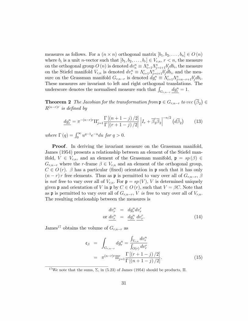
Theorem 2 The Jacobian for the transformation from p 2 Gr;n�r to vec��2�2
R(n�r)r is de�ned by
dgnr = ��(n�r)r�rj=1� [(n+ 1� j) =2]
� [(r + 1� j) =2]
���Ir + �02�2
����n=2 �d�2� (13)
where � (q) =R10uq�1e�udu for q > 0:
Proof . In deriving the invariant measure on the Grassman manifold,James (1954) presents a relationship between an element of the Stiefel man-ifold, V 2 Vr;n; and an element of the Grassman manifold, p = sp (�) 2Gr;n�r where the r-frame � 2 Vr;n and an element of the orthogonal group,C 2 O (r). � has a particular (�xed) orientation in p such that it has only(n� r) r free elements. Thus as p is permitted to vary over all of Gr;n�r, �is not free to vary over all of Vr;n: For p = sp (V ), V is determined uniquelygiven p and orientation of V in p by C 2 O (r), such that V = �C: Note thatas p is permitted to vary over all of Gr;n�r, V is free to vary over all of Vr;n:The resulting relationship between the measures is
dvnr = dgnr dvrr
or dvnr = dgnr dvrr : (14)
James17 obtains the volume of Gr;n�r as
c� =
ZGr;n�r
dgnr =
RVr;n
dvnrRO(r)
dvrr
= �(n�r)r�rj=1� [(r + 1� j) =2]
� [(n+ 1� j) =2]: (15)
17We note that the sums, �; in (5.23) of James (1954) should be products, �:
31

Since the polynomial term accompanying the exterior product of the dif-ferential forms is equivalent to the Jacobian for the transformation (Muirhead1982, Theorem 2.1.1), we can see from the expression (14) that the Jacobianfor the transformation V to (�;C) is one.Next consider the transformation from V 2 Vr;n; to �2 2 R(n�r)r and
C 2 O (r) presented by Phillips (1989 and 1994, Lemma 5.2 and see alsoChikuse, 1998) and reproduced here:
V =�c0 + c0?�2
� hIr + �
02�2
i�1=2C:
The di¤erential form for this transformation is
dvnr = ��(n�r)r�rj=1� [(n+ 1� j) =2]
� [(r + 1� j) =2]
���Ir + �02�2
����n=2 d�2 �dvrr� (16)
(Phillips, 1989, 1994).Equating (14) and (16) gives the result. Another, slightly more general
proof for the same result is presented in Chikuse (1998).�To avoid using linear restrictions with a normalisation to identify � it
is necessary to �nd an alternative set of restrictions that do not requireknowledge of c and which avoid the issues associated with the posterior for�2: Fortunately the de�nition (14) and the discussion in the proof of The-orem 2 provides a natural solution to this question. That is use � 2 Vr;nwhich implies r (r + 1) =2 restrictions. The dimension of the Grassman man-ifold is only (n� r) r while the dimension of the Stiefel manifold Vr;n isnr � r (r + 1) =2, which exceeds that of Gr;n�r by r (r � 1) =2: In (14), theseremaining restrictions come from the orientation of � in p by C 2 O (r). Theprior, the posterior (as is made clear later) and the di¤erential form for �are all invariant to translations of the form � ! �H; H 2 O (r) : Thereforeit is possible to work directly with � as an element of the Stiefel manifold
and adjust the integrals with respect to � by�R
O(r)dvrr
��1. Note that these
identifying restrictions do not distort the weight on the space of the parame-ter of interest, p, and it is never necessary to actually specify the orientationof � in p.Next we provide a proof that linear identifying restrictions with a �at
prior give zero weight to the chosen linear restrictions. The Jacobian de�nedby (13) implies that a �at prior on p is informative with respect to �2 andvice versa. This leads us to consider the implications of a �at prior on �2 forthe prior on p.
32

Theorem 3 The Jacobian for the transformation from �2 2 R(n�r)r to p 2Gr;n�r is de�ned by�d�2
�= �(n�r)r�rj=1
� [(r + 1� j) =2]
� [(n+ 1� j) =2]
��Ir + (c�)0�1 �0c0?c?� (c�)�1��n=2 (dgnr )= J dgnr : (17)
Proof . Invert (16) and replace �2 by c?� (c�)�1.�
The following proof demonstrates the claim in Section 3.2 that assumingwe know which rows of � are linearly independent so as to impose linearidentifying restrictions makes this assumption a priori impossible.
Theorem 4 Given r; use of the normalisation �2 = c?� (c�)�1 results in
a transformation of measures for the transformation �2 2 R(n�r)r ! p 2Gr;n�r that places in�nite mass in the region of null space of c relative to thecomplement of this region.
Proof . Let �c? be the plane de�ned by the null space of c. De�nea ball, B, of �xed diameter, d, around �c? and let N0 = B \ Gr;n�r andN = Gr;n�r �N0. Since for d > 0,
RNJdgnr is �nite whereas
RN0Jdgnr = 1,
we have RN0JdgnrR
NJdgnr
=1:
�Discussion: Essentially, the Jacobian for �2 ! p places in�nitely more
weight in the direction where c� is singular. Thus, normalisation of � bychoice of c with a �at prior on �2 implies in�nite prior odds against thisnormalisation.To demonstrate this result, consider a n�dimensional system for y =
(x0; z0)0 where x is a r vector. To implement linear restrictions a normalisationmust begin by �rst choosing c. Suppose it is believed that if a cointegratingrelationship exists then it will most likely involve the elements of x in linearlyindependent relations: That is in y� = x�1+ z�2 v I (0), det (�1) is believedfar from zero making it safe to normalise on �1; and so choose c = [Ir 0] andestimate �2 = c?� (c�)
�1 :From (17) we see as p = sp (�)! sp (c) ; c?� ! 0(n�r)�r and c� ! O (r)
and J ! 1. However, as vectors in � approach the null space of c, that isdet (c�) ! 0; then (c�)�1 ! 1; and thus J ! 1. As a result the prior
33

will more heavily weight regions where det (c�) = det (�1) t 0; contrary tothe intention of the economist. As a trivial example, consider our moneydemand study with r = 1 and �t = �1mt + �2inct: If we believe money ismost likely to enter the cointegrating relation, we would choose c = (1; 0)as we believe �1 6= 0: Yet the Jacobian places in�nite weight in the region�1 = 0 excluding mt from the cointegrating relation.To support the use of model averaging in this application, we provide
here proofs that the posterior will be proper and all �nite moments of �exist. Since g! (in (8)) is �nite for the class of priors considered, for theBayes factor to be �nite requires the integral with respect to � to be �nite.The following are some general results with respect to this integral.
Theorem 5 The marginal posterior density for � conditional upon ! hasthe same form for each model considered:
p (�jM!; y) _ j�0D0�j�T=2 j�0D1�j(T�n)=2 (18)
= k� (�jM!; y)
where k� (�jM!; y) = j�0D0�j�T=2 j�0D1�j(T�n)=2 :
Theorem 6 The marginal posterior density for � conditional upon ! in (18)is proper and all �nite moments exist.
Proof . Denote by bij any element of �: The proof follows from the resultthat the integral
M� =
ZVr;n
jbijjm k� (�) dvnr
for m = 0; 1; 2; : : : is bounded above almost everywhere by the �nite integralMR 1�1 jbijj
m dbij. As the elements of �, bij, have compact support, it is onlynecessary for this proof to show that k� (�) dvnr is bounded above almosteverywhere by some �nite constant function over Vr;n (note the adjustmentto the integral over Gr;n�r simply requires division by the �nite volume ofO (r) ; thus we only need consider the integral over Vr;n). As demonstratedin the proof to Theorem 2 above, dgnr is integrable and therefore boundedabove almost everywhere by some �nite constant,M1.The eigenvalues �j (Dl) for l = 0; 1; will be positive and �nite with prob-
ability one. By the Poincaré separation theorem, since � 2 Vr;n; then
�rj=1�n�r+j (Dl) � j�0D1�j � �rj=1�j (Dl)
34

and so k� (�) is bounded above (and below) by some positive �nite constant,M2. Thus k� (�) dgnr has a �nite upper bound, M = M1M2: With thecompact support for bij; these conditions are su¢ cient to ensure the posteriorfor � will be proper and all �nite moments exist (see Billingsley 1979, pp.174 and 180).�
35

0.63
0.55
0.47
0.38
0.30
0.22
0.13
0.05
0.03
0.12
0 6 12 18 24 30 36 42 48 54 60
00.2 0.20.4 0.40.6
0.60.8 0.81
1.00
0.72
0.44
0.16
0.1
2
0.3
9
0.6
7
h=10h=30h=60
Figure 1: This �gure shows the densities over 60 periods of the impulse re-sponses of consumption to a permanent shock. The upper panel shows the20% (0-0.2), 40% (0.2-0.4), 60% (0.4-0.6) and 80% (0.6-0.8) highest posteriordensity intervals. The lower panel shows the density pro�les for the impulseresponse at h = 10; 30 and 60 periods into the future.
36

4.96
4.54
4.12
3.71
3.29
2.87
2.45
2.04
1.62
1.20
0.79
0.370 6 12 18 24 30 36 42 48 54 60
00.2 0.20.4 0.40.6
0.60.8 0.81
7.05
5.66
4.26
2.87
1.48
0.09
1.3
0
h=10h=30h=60
Figure 2: This �gure shows the densities over 60 periods of the impulseresponses of investment to a permanent shock. The upper panel shows the20% (0-0.2), 40% (0.2-0.4), 60% (0.4-0.6) and 80% (0.6-0.8) highest posteriordensity intervals. The lower panel shows the density pro�les for the impulseresponse at h = 10; 30 and 60 periods into the future.
37

1.38
1.24
1.11
0.98
0.84
0.71
0.58
0.44
0.31
0.18
0.04
0.090 6 1 2 1 8 24 30 36 42 4 8 5 4 60
0 0.2 0.20 .4 0 .40.60 .6 0.8 0.81
1.61
1.28
0.94
0.61
0.28
0.0
6
0.3
9
h=10h=30h=60
Figure 3: This �gure shows the densities over 60 periods of the impulseresponses of income to a permanent shock. The upper panel shows the20% (0-0.2), 40% (0.2-0.4), 60% (0.4-0.6) and 80% (0.6-0.8) highest posteriordensity intervals. The lower panel shows the density pro�les for the impulseresponse at h = 10; 30 and 60 periods into the future.
38