Embed Size (px)
Citation preview
Rocket Based Combined Cycle
Exchange Inlet Performance Estimation at
Supersonic Speeds
by
Aliaksandr Murzionak
A Thesis submitted to
the Faculty of Graduate Studies and Research
in partial fulfilment of
the requirements for the degree of
Master of Applied Science
in
Aerospace Engineering
Department of Mechanical and Aerospace Engineering
Carleton University
Ottawa, Ontario, Canada
January 2013
Copyright c©
2013 - Aliaksandr Murzionak
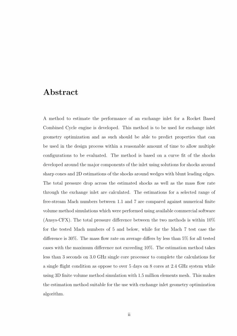
Abstract
A method to estimate the performance of an exchange inlet for a Rocket Based
Combined Cycle engine is developed. This method is to be used for exchange inlet
geometry optimization and as such should be able to predict properties that can
be used in the design process within a reasonable amount of time to allow multiple
configurations to be evaluated. The method is based on a curve fit of the shocks
developed around the major components of the inlet using solutions for shocks around
sharp cones and 2D estimations of the shocks around wedges with blunt leading edges.
The total pressure drop across the estimated shocks as well as the mass flow rate
through the exchange inlet are calculated. The estimations for a selected range of
free-stream Mach numbers between 1.1 and 7 are compared against numerical finite
volume method simulations which were performed using available commercial software
(Ansys-CFX). The total pressure difference between the two methods is within 10%
for the tested Mach numbers of 5 and below, while for the Mach 7 test case the
difference is 30%. The mass flow rate on average differs by less than 5% for all tested
cases with the maximum difference not exceeding 10%. The estimation method takes
less than 3 seconds on 3.0 GHz single core processor to complete the calculations for
a single flight condition as oppose to over 5 days on 8 cores at 2.4 GHz system while
using 3D finite volume method simulation with 1.5 million elements mesh. This makes
the estimation method suitable for the use with exchange inlet geometry optimization
algorithm.
ii

Acknowledgments
I would like to thank my supervisor, professor J. Etele, for guiding me towards the
completion of this work. I would also like to thank my colleagues for providing me
with good advices.
I am very grateful to my family who were always supportive through my years of
education and who made this work possible. A special thanks to my brother, who,
despite his tight schedule at the time, managed to thoroughly go through this thesis
and provide with constructive feedback.
iii
Table of Contents
Abstract ii
Acknowledgments iii
Table of Contents iv
List of Tables vi
List of Figures vii
List of Acronyms x
List of Symbols xi
1 Introduction 1
1.1 Overview . . . . . . . . . . . . . . . . . . . . . . . . . . . . . . . . . . 1
1.2 RBCC . . . . . . . . . . . . . . . . . . . . . . . . . . . . . . . . . . . 4
1.3 Problem Statement . . . . . . . . . . . . . . . . . . . . . . . . . . . . 9
1.4 Computational Methods . . . . . . . . . . . . . . . . . . . . . . . . . 10
1.4.1 Navier-Stokes Solver . . . . . . . . . . . . . . . . . . . . . . . 11
1.4.2 Method of Characteristics . . . . . . . . . . . . . . . . . . . . 12
1.4.3 Semi-Analytical Method . . . . . . . . . . . . . . . . . . . . . 13
2 Exchange Inlet Geometry 15
iv
3 Estimation Method 18
3.1 Overview . . . . . . . . . . . . . . . . . . . . . . . . . . . . . . . . . . 18
3.2 Isentropic compressible flow and oblique shock equations . . . . . . . 21
3.3 Centre Body Shock Estimation . . . . . . . . . . . . . . . . . . . . . 25
3.4 Fairings Shock Estimation . . . . . . . . . . . . . . . . . . . . . . . . 28
3.5 Cowl Shock Estimation . . . . . . . . . . . . . . . . . . . . . . . . . . 35
3.6 Mass Flow Rate Estimation . . . . . . . . . . . . . . . . . . . . . . . 46
4 2D CFD simulations 49
4.1 2D geometry . . . . . . . . . . . . . . . . . . . . . . . . . . . . . . . . 49
4.2 Domain, Mesh and Simulation setup . . . . . . . . . . . . . . . . . . 50
4.3 Grid Sensitivity Study . . . . . . . . . . . . . . . . . . . . . . . . . . 55
4.4 Results and comparison . . . . . . . . . . . . . . . . . . . . . . . . . 58
5 3D CFD simulations 63
5.1 Overview . . . . . . . . . . . . . . . . . . . . . . . . . . . . . . . . . . 63
5.2 3D Simulation Setup . . . . . . . . . . . . . . . . . . . . . . . . . . . 63
5.3 Grid sensitivity analysis . . . . . . . . . . . . . . . . . . . . . . . . . 69
5.4 Results and comparison . . . . . . . . . . . . . . . . . . . . . . . . . 72
5.4.1 Shock geometry . . . . . . . . . . . . . . . . . . . . . . . . . . 72
5.4.2 Total pressure . . . . . . . . . . . . . . . . . . . . . . . . . . . 79
5.4.3 Mass flow rate . . . . . . . . . . . . . . . . . . . . . . . . . . . 82
6 Conclusions and Recommendations 85
6.1 Conclusions . . . . . . . . . . . . . . . . . . . . . . . . . . . . . . . . 85
6.2 Recommendations . . . . . . . . . . . . . . . . . . . . . . . . . . . . . 86
List of References 88
v

List of Tables
3.1 Summary of angles used for the shock-expansion wave interaction cal-
culations. . . . . . . . . . . . . . . . . . . . . . . . . . . . . . . . . . 44
4.1 List of meshes for 2D simulations. . . . . . . . . . . . . . . . . . . . . 55
4.2 Grid convergence summary. . . . . . . . . . . . . . . . . . . . . . . . 55
5.1 Flight Conditions. . . . . . . . . . . . . . . . . . . . . . . . . . . . . . 66
5.2 List of meshes for 3D grid convergence study . . . . . . . . . . . . . . 69
5.3 Grid convergence summary. . . . . . . . . . . . . . . . . . . . . . . . 71
5.4 Pressure ratio difference. . . . . . . . . . . . . . . . . . . . . . . . . . 81
5.5 Mass flow rate percent difference. . . . . . . . . . . . . . . . . . . . . 83
vi

List of Figures
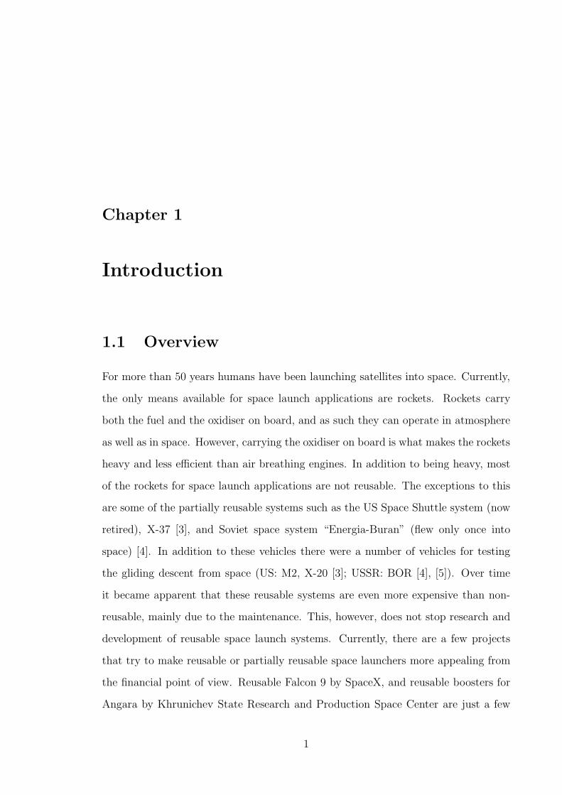
1.1 Approximate specific impulse performance of different propulsion cy-
cles (modified from [1], with additional information from [2]). . . . . . 2
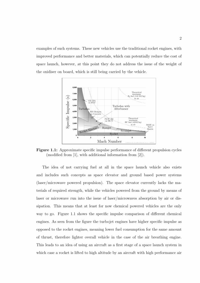
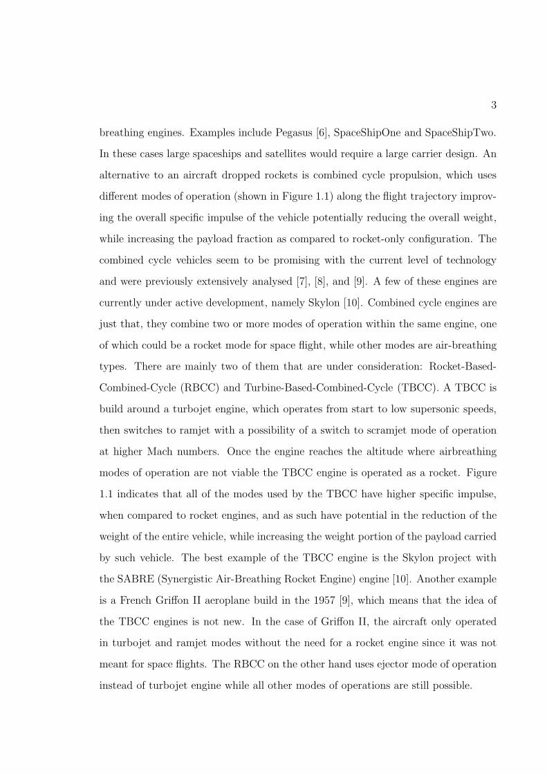
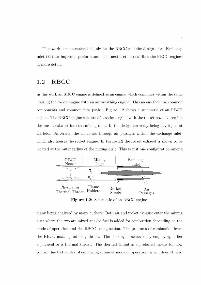
1.2 Schematic of an RBCC engine. . . . . . . . . . . . . . . . . . . . . . 4
1.3 Modes of operation of an RBCC engine. . . . . . . . . . . . . . . . . 5
2.1 Cutaway view of EI geometry. . . . . . . . . . . . . . . . . . . . . . . 15
2.2 Definition of half-section of the EI and the symmetry planes. . . . . . 17
2.3 Section of EI geometry as imported into the estimation code. . . . . . 17
3.1 Main shocks generated by the geometry . . . . . . . . . . . . . . . . . 19
3.2 Supersonic expansion around a corner. . . . . . . . . . . . . . . . . . 22
3.3 Oblique shock nomenclature. . . . . . . . . . . . . . . . . . . . . . . . 23
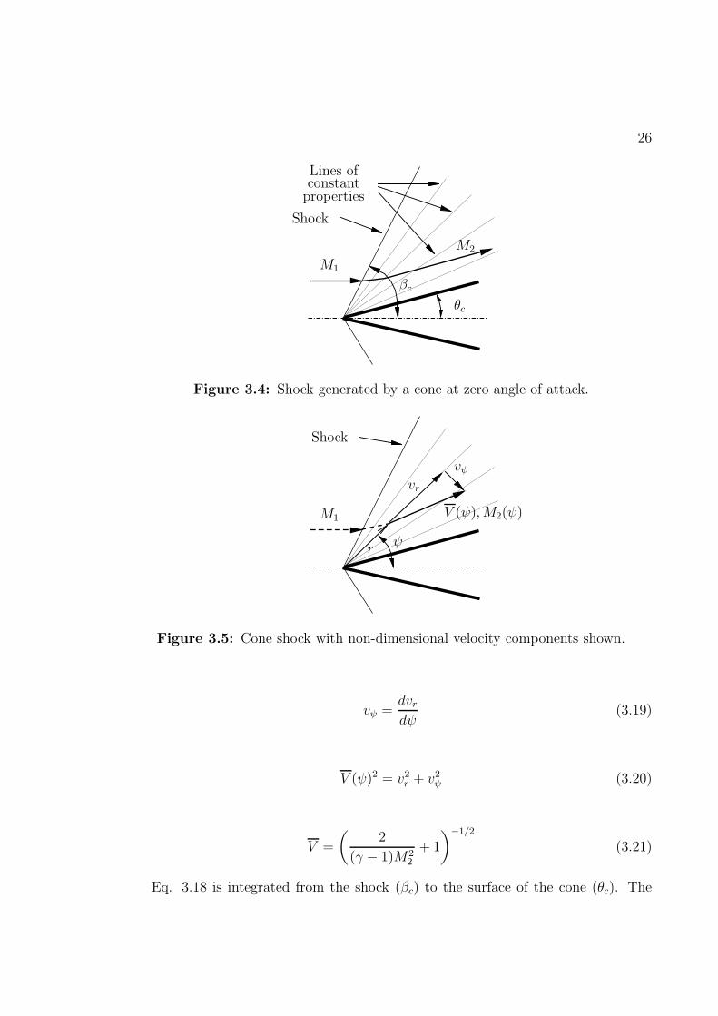
3.4 Shock generated by a cone at zero angle of attack. . . . . . . . . . . . 26
3.5 Cone shock with non-dimensional velocity components shown. . . . . 26
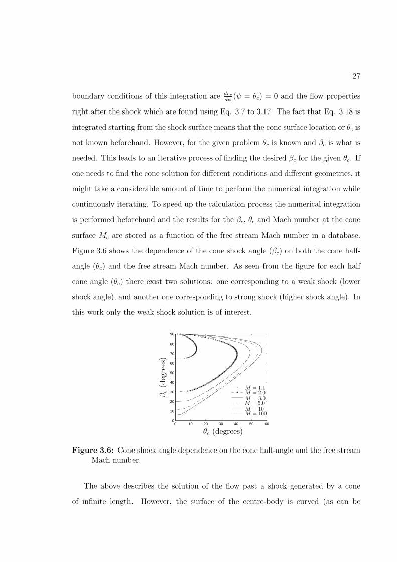
3.6 Cone shock angle dependence on the cone half-angle and the free
stream Mach number. . . . . . . . . . . . . . . . . . . . . . . . . . . . 27
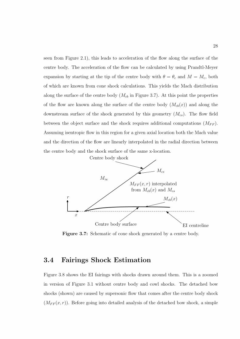
3.7 Schematic of cone shock generated by a centre body. . . . . . . . . . 28
3.8 Shock generated by the fairing. . . . . . . . . . . . . . . . . . . . . . 29
3.9 Shock generated by a wedge. . . . . . . . . . . . . . . . . . . . . . . . 29
3.10 Variables used to determine detached shock geometries. . . . . . . . . 31
3.11 Shock generated by the fairing with shock-plane shown. . . . . . . . . 34
3.12 Flow acceleration around the fairing. . . . . . . . . . . . . . . . . . . 35
vii
3.13 Possible reflection shocks. . . . . . . . . . . . . . . . . . . . . . . . . 37
3.14 Variables required for Mach reflection analysis. . . . . . . . . . . . . . 38
3.15 Mach reflection. . . . . . . . . . . . . . . . . . . . . . . . . . . . . . . 40
3.16 Side view of cowl shock structure. . . . . . . . . . . . . . . . . . . . . 41
3.17 Shock/Expansion wave intersection (numbers in brackets indicate the
regions shown in Figure 3.16 from previous analysis). . . . . . . . . . 43
3.18 Variables needed for the calculation of the mass flow rate through EI. 46
3.19 Half-section with the variables for area calculations. . . . . . . . . . . 47
4.1 Simple 2D geometry. . . . . . . . . . . . . . . . . . . . . . . . . . . . 49
4.2 2D domain with boundary conditions shown (R = 0.1 m). . . . . . . 50
4.3 Examples of the mesh for 2D CFD simulations (R = 0.01 m). . . . . . 52
4.4 Mach gradient distribution along the symmetry plane for different mesh
sizes (M∞ = 1.1). . . . . . . . . . . . . . . . . . . . . . . . . . . . . . 53
4.5 Plot of Residuals (M∞ = 2.0). . . . . . . . . . . . . . . . . . . . . . . 54
4.6 Stand-off distance as a function of the mesh size. . . . . . . . . . . . 56
4.7 Mach distribution along the symmetry plane. . . . . . . . . . . . . . . 57
4.8 Mach gradient distribution along the symmetry plane (M∞ = 2.0). . . 57
4.9 Shock stand-off distance vs Mach number. . . . . . . . . . . . . . . . 58
4.10 Shape of the shocks produced by a blunt body at different Mach num-
bers (R = 0.1 m). . . . . . . . . . . . . . . . . . . . . . . . . . . . . . 59
4.11 Shape of the shocks produced by a blunt body at different Mach num-
bers (R = 0.01 m). . . . . . . . . . . . . . . . . . . . . . . . . . . . . 60
4.12 Shape of the shocks produced by a blunt body at different Mach num-
bers, for CFD θ = 0 deg, while for Billig and Estimations θ = 3 deg
(R = 0.01 m). . . . . . . . . . . . . . . . . . . . . . . . . . . . . . . . 61
4.13 Shape of the shocks produced by a blunt body with different deflection
angles (R = 0.01 m, M∞ = 2.0). . . . . . . . . . . . . . . . . . . . . . 62
viii
4.14 Contour plot of the flow direction for (R = 0.01 m, M∞ = 2.0). . . . . 62
5.1 Half-section of the EI used for 3D simulations with symmetry planes
shown. . . . . . . . . . . . . . . . . . . . . . . . . . . . . . . . . . . . 64
5.2 The domain setup for CFD simulations with boundaries shown. . . . 64
5.3 Centre body tip geometry. . . . . . . . . . . . . . . . . . . . . . . . . 65
5.4 Simulated flight profile. . . . . . . . . . . . . . . . . . . . . . . . . . . 65
5.5 Plot of Residuals (M∞ = 2.0). . . . . . . . . . . . . . . . . . . . . . . 67
5.6 Test locations for the time and grid convergence checks. . . . . . . . . 67
5.7 Time Convergence (Coarse Mesh, M∞ = 2.0). . . . . . . . . . . . . . 68
5.8 Time Convergence (Fine Mesh, M∞ = 2.0). . . . . . . . . . . . . . . . 70
5.9 Grid Convergence. . . . . . . . . . . . . . . . . . . . . . . . . . . . . 72
5.10 Shock geometries obtained from 3D CFD simulations. . . . . . . . . . 73
5.11 Cowl shock (M∞ = 7). . . . . . . . . . . . . . . . . . . . . . . . . . . 74
5.12 Mach distribution (Symmetry Plane 1) with lines representing the es-
timated shocks. . . . . . . . . . . . . . . . . . . . . . . . . . . . . . . 76
5.13 Fairing shock location and its projection to Symmetry Plane 1. . . . . 77
5.14 Mach distribution after the fairing shock (Selected Planes). . . . . . . 78
5.15 Mach number along the centre body surface (estimation line ends at
the location of the fairing shock). . . . . . . . . . . . . . . . . . . . . 79
5.16 Pressure loss through the intake with cumulative total pressure after
each shock shown. . . . . . . . . . . . . . . . . . . . . . . . . . . . . . 79
5.17 Example of averaging locations for total pressure comparison (M∞ =
2.0). . . . . . . . . . . . . . . . . . . . . . . . . . . . . . . . . . . . . 80
5.18 Pressure ratio difference. . . . . . . . . . . . . . . . . . . . . . . . . . 82
5.19 Estimations of the mass flow rate. . . . . . . . . . . . . . . . . . . . . 83
5.20 Mass flow rate comparison. . . . . . . . . . . . . . . . . . . . . . . . . 84
5.21 Mass flow rate percent difference. . . . . . . . . . . . . . . . . . . . . 84
ix
List of Acronyms
Acronyms Definition
CFD Computation Fluid Dynamics
DAB Diffusion and Afterburning
EI Exchange Inlet
FVM Finite Volume Method
HR High Resolution advection scheme
ODE Ordinary Differential Equation
RBCC Rocket Based Combined Cycle
RMS Root Mean Square
SMC Simultaneous Mixing and Combustion
wrt with respect to
x
List of Symbols
Symbols Definition
a Distance from the coordinate origin to the vertex of a hy-
perbole [m]
ds Shock stand-off distance [m]
m Mass flow rate [kg/s]
r Radial position [m]
v Non-dimensional velocity component
x x coordinate [m]
y y coordinate [m]
A Area [m2]
M Mach number
P Static pressure [Pa]
Po Total Pressure [Pa]
R Radius [m]
xi
Rair Gas constant (air) [J/kg/K]
T Static Temperature [K]
To Total Temperature [K]
V Velocity [m/s]
V Non-dimensional velocity
β Shock angle [rad]
γ Ratio of specific heats
ǫ Eccentricity of a hyperbole
ν Prandtl-Meyer function
θ Flow deflection angle / Flow direction angle [rad]
ρ Density [kg/m3]
τ Mach wave angle [rad]
ψ Angle of the ray of constant properties for flows around
cones [rad]
Superscript
∗ Throat/choked conditions
′ Direction with respect to horizontal line
Subscript
1 Conditions before a shock
xii
2 Conditions after a shock
c Cone
cb Centre body
cw Cowl
d Near-detached shock conditions
i Incident shock
n Normal component of velocity/Mach
o Stagnation conditions
r Reflected shock / radial component
t Tangential component of velocity/Mach
s Shock
ss Slipstream
w Wedge
∞ Free stream conditions
FF Flow Field
xiii
Chapter 1
Introduction
1.1 Overview
For more than 50 years humans have been launching satellites into space. Currently,
the only means available for space launch applications are rockets. Rockets carry
both the fuel and the oxidiser on board, and as such they can operate in atmosphere
as well as in space. However, carrying the oxidiser on board is what makes the rockets
heavy and less efficient than air breathing engines. In addition to being heavy, most
of the rockets for space launch applications are not reusable. The exceptions to this
are some of the partially reusable systems such as the US Space Shuttle system (now
retired), X-37 [3], and Soviet space system “Energia-Buran” (flew only once into
space) [4]. In addition to these vehicles there were a number of vehicles for testing
the gliding descent from space (US: M2, X-20 [3]; USSR: BOR [4], [5]). Over time
it became apparent that these reusable systems are even more expensive than non-
reusable, mainly due to the maintenance. This, however, does not stop research and
development of reusable space launch systems. Currently, there are a few projects
that try to make reusable or partially reusable space launchers more appealing from
the financial point of view. Reusable Falcon 9 by SpaceX, and reusable boosters for
Angara by Khrunichev State Research and Production Space Center are just a few
1
2
examples of such systems. These new vehicles use the traditional rocket engines, with
improved performance and better materials, which can potentially reduce the cost of
space launch, however, at this point they do not address the issue of the weight of
the oxidiser on board, which is still being carried by the vehicle.
Mach Number
SpecificIm
pulse(s)
Theoreticalmaximum
H2 fuel (143 MJ/kg)in air
Theoreticalmaximum
HC fuel (42MJ/kg)in air
RocketRocket Ej
ector ScramjetRamjet
Turbofan
GE CF6on B747
RR Olympuson Concorde
P&W J58on SR-71
SSME onSpaceShuttle
Turbofan withAfterburner
Figure 1.1: Approximate specific impulse performance of different propulsion cycles(modified from [1], with additional information from [2]).
The idea of not carrying fuel at all in the space launch vehicle also exists
and includes such concepts as space elevator and ground based power systems
(laser/microwave powered propulsion). The space elevator currently lacks the ma-
terials of required strength, while the vehicles powered from the ground by means of
laser or microwave run into the issue of laser/microwaves absorption by air or dis-
sipation. This means that at least for now chemical powered vehicles are the only
way to go. Figure 1.1 shows the specific impulse comparison of different chemical
engines. As seen from the figure the turbojet engines have higher specific impulse as
opposed to the rocket engines, meaning lower fuel consumption for the same amount
of thrust, therefore lighter overall vehicle in the case of the air breathing engine.
This leads to an idea of using an aircraft as a first stage of a space launch system in
which case a rocket is lifted to high altitude by an aircraft with high performance air
3
breathing engines. Examples include Pegasus [6], SpaceShipOne and SpaceShipTwo.
In these cases large spaceships and satellites would require a large carrier design. An
alternative to an aircraft dropped rockets is combined cycle propulsion, which uses
different modes of operation (shown in Figure 1.1) along the flight trajectory improv-
ing the overall specific impulse of the vehicle potentially reducing the overall weight,
while increasing the payload fraction as compared to rocket-only configuration. The
combined cycle vehicles seem to be promising with the current level of technology
and were previously extensively analysed [7], [8], and [9]. A few of these engines are
currently under active development, namely Skylon [10]. Combined cycle engines are
just that, they combine two or more modes of operation within the same engine, one
of which could be a rocket mode for space flight, while other modes are air-breathing
types. There are mainly two of them that are under consideration: Rocket-Based-
Combined-Cycle (RBCC) and Turbine-Based-Combined-Cycle (TBCC). A TBCC is
build around a turbojet engine, which operates from start to low supersonic speeds,
then switches to ramjet with a possibility of a switch to scramjet mode of operation
at higher Mach numbers. Once the engine reaches the altitude where airbreathing
modes of operation are not viable the TBCC engine is operated as a rocket. Figure
1.1 indicates that all of the modes used by the TBCC have higher specific impulse,
when compared to rocket engines, and as such have potential in the reduction of the
weight of the entire vehicle, while increasing the weight portion of the payload carried
by such vehicle. The best example of the TBCC engine is the Skylon project with
the SABRE (Synergistic Air-Breathing Rocket Engine) engine [10]. Another example
is a French Griffon II aeroplane build in the 1957 [9], which means that the idea of
the TBCC engines is not new. In the case of Griffon II, the aircraft only operated
in turbojet and ramjet modes without the need for a rocket engine since it was not
meant for space flights. The RBCC on the other hand uses ejector mode of operation
instead of turbojet engine while all other modes of operations are still possible.
4
This work is concentrated mainly on the RBCC and the design of an Exchange
Inlet (EI) for improved performance. The next section describes the RBCC engines
in more detail.
1.2 RBCC
In this work an RBCC engine is defined as an engine which combines within the same
housing the rocket engine with an air breathing engine. This means they use common
components and common flow paths. Figure 1.2 shows a schematic of an RBCC
engine. The RBCC engine consists of a rocket engine with the rocket nozzle directing
the rocket exhaust into the mixing duct. In the design currently being developed at
Carleton University, the air comes through air passages within the exchange inlet,
which also houses the rocket engine. In Figure 1.2 the rocket exhaust is shown to be
located at the outer radius of the mixing duct. This is just one configuration among
ExchangeInlet
MixingDuct
RBCCNozzle
AirPassages
RocketNozzle
FlameHolders
Physical orThermal Throat
Figure 1.2: Schematic of an RBCC engine.
many being analysed by many authors. Both air and rocket exhaust enter the mixing
duct where the two are mixed and/or fuel is added for combustion depending on the
mode of operation and the RBCC configuration. The products of combustion leave
the RBCC nozzle producing thrust. The choking is achieved by employing either
a physical or a thermal throat. The thermal throat is a preferred means for flow
control due to the idea of employing scramjet mode of operation, which doesn’t need
5
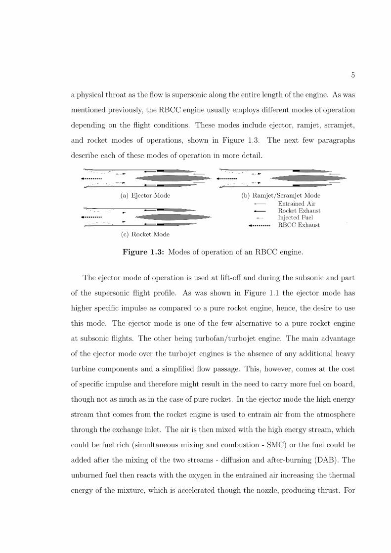
a physical throat as the flow is supersonic along the entire length of the engine. As was
mentioned previously, the RBCC engine usually employs different modes of operation
depending on the flight conditions. These modes include ejector, ramjet, scramjet,
and rocket modes of operations, shown in Figure 1.3. The next few paragraphs
describe each of these modes of operation in more detail.
(a) Ejector Mode (b) Ramjet/Scramjet Mode
(c) Rocket Mode
Entrained AirRocket ExhaustInjected FuelRBCC Exhaust
Figure 1.3: Modes of operation of an RBCC engine.
The ejector mode of operation is used at lift-off and during the subsonic and part
of the supersonic flight profile. As was shown in Figure 1.1 the ejector mode has
higher specific impulse as compared to a pure rocket engine, hence, the desire to use
this mode. The ejector mode is one of the few alternative to a pure rocket engine
at subsonic flights. The other being turbofan/turbojet engine. The main advantage
of the ejector mode over the turbojet engines is the absence of any additional heavy
turbine components and a simplified flow passage. This, however, comes at the cost
of specific impulse and therefore might result in the need to carry more fuel on board,
though not as much as in the case of pure rocket. In the ejector mode the high energy
stream that comes from the rocket engine is used to entrain air from the atmosphere
through the exchange inlet. The air is then mixed with the high energy stream, which
could be fuel rich (simultaneous mixing and combustion - SMC) or the fuel could be
added after the mixing of the two streams - diffusion and after-burning (DAB). The
unburned fuel then reacts with the oxygen in the entrained air increasing the thermal
energy of the mixture, which is accelerated though the nozzle, producing thrust. For
6
higher efficiency of the ejector mode a good mixing between the rocket and air streams
is required. A longer mixing duct allows for better mixing, however, it also means
a heavier engine, so a compromise between the two is required. There are different
ways to improve the mixing of the two streams. One is the pulsing rocket stream [11].
Another way is to increase the area of interaction between the streams, as is done by
multiple rocket engines. Both of these methods were extensively analysed by different
authors, who came to conclusion that it is possible to reduce the length of the mixing
duct to a length over diameter ratio (L/D) of 2.5 [12]. The simplest design with
the rocket being in the center showed a good mixing at L/D of around 8 to 10 [13].
This means that with proper configuration of the rocket streams, it is possible to
considerably reduce the length of the mixing duct. In Figure 1.2 and 1.3 the fuel is
shown to be injected inside the mixing chamber. This fuel injection is not required
for the case of SMC. In the case of DAB, some authors suggest a premixing of the
fuel and air even before the air enters the mixing chamber. Even though there are
many studies on the topic of rocket ejectors, their application is relatively scarce.
This cannot be said about the next mode of operation which takes over the ejector
mode at higher speeds - ramjet.
At speeds above Mach 2 but below Mach 5-7 the ramjet mode of operation can be
used to propel the RBCC engine (Figure 1.3b). Although it was shown that ramjets
could be used even at low subsonic speeds they were found to be inefficient until
supersonic speeds [9] and they cannot operate at standstill, hence the need for an
initial acceleration mode, which in the case of an RBCC engine is the rocket ejector.
A ramjet is probably the simplest airbreathing engine known. It can be as simple
as a pipe with a nozzle at the end, plus a fuel injection system. For a more efficient
ramjet engine a bit more elaborated design is needed. The ramjet intake is designed
to slow down the oncoming air and convert the dynamic pressure to static pressure
(ram effect) for more efficient combustion. At low speeds dynamic pressure is low and
7
as such the rise in the static pressure is also low which explains the ramjet inefficiency
at low speeds. Once air is compressed the fuel is added and the thrust is generated. In
this mode the high energy rocket stream is not required (though can be used), which
simplifies the analysis of the engine. For supersonic flights the compression happens
through the series of shocks generated by the intake structure, which slows the air to
subsonic speeds. These shocks need to be taken into account during the design stage.
Unfortunately, at higher Mach numbers (above Mach 5-7) the deceleration of the air
to subsonic would result in static temperatures in excess of the 2000 K, which is above
the limit of many known materials, and the combustion at these temperatures would
be limited due to dissociation of the molecules [14]. As such, the airflow is decelerated
to lower supersonic speeds. Since the airflow is supersonic the combustion happens
at supersonic or mixed supersonic/subsonic speeds, meaning the mode of operation
is scramjet (which means supersonic combustion ramjet). This leads to additional
challenges, which will not be described here. For more information on scramjets the
reader is directed to [15].
The concept of ramjet engine came to light in early 1900s, with further testing and
development in the next years in many parts of Europe (France, Germany, Hungary,
Russia and UK) and US [9]. Since then ramjets have been used to power jets (Griffin
II) and many missiles (V-1, SA-4, VEGA, X-7) as early as the 1930s. Since ramjets
are unable to work from a standstill they have to be initially propelled forward by
other means. In the case of the RBCC engines the ejector mode of operation is used.
In the case of the Griffin II the aircraft is propelled by a turbojet engine, while in
the case of the missiles usually a solid rocket motor is used to initially propel them
to the supersonic speed. In the 1960s the work was done on the inter continental
ballistic missile to use ramjet technology - Gnom [16]. The missile was considerably
lighter than equivalent solid-fuel or liquid-fuel rocket. However, the rocket was never
completed due to the death of the chief designer. After a few ground tests the project

8
was cancelled. As seen from the above examples the ramjet technology is quiet mature
with an extensive use in military applications.
The scramjet technology on the other hand is still in development. Currently,
there is extensive research being performed in the area of supersonic combustion and
scramjet vehicles, with major research being done in Europe and Russia, Japan, and
USA. However in all of these research works, the engines are accelerated to hypersonic
speeds by means of solid rockets. To date research in scramjet propulsion has led to
the creation of the X-43A achieving Mach 9.8 powered by scramjet engine [17].
The final mode of operation of the RBCC engine is the rocket mode. In the case of
non-combined cycles, the rocket engines operate at either over-expanded (the nozzle
pressure is slightly lower than atmospheric pressure) or under-expanded (the nozzle
pressure is slightly higher than atmospheric pressure) nozzle exit conditions. Neither
of the conditions represent the maximum nozzle efficiency of the rocket. At higher
altitudes the atmospheric pressure is much lower than that at lower altitude, meaning
that if the rocket nozzle is designed to operate in the lower atmosphere it is going
to be under-expanded in the higher atmosphere. Under-expansion means that it is
still possible to accelerate the flow further, which is to improve the performance of
the nozzle. In the case of the rockets one reason for multi-staging is to bring the
nozzle conditions closer to the local atmospheric. In the case of the RBCC engine,
the rocket mode is activated in the higher atmosphere where pressure is negligible.
This means that the rocket exhaust, after leaving the rocket nozzle (Figure 1.3c)
continues to expand, achieving higher speeds at the RBCC nozzle exit, which means
higher performance of the engine.
From a theoretical perspective the RBCC engine has a higher overall specific im-
pulse and therefore better performance than an equivalent rocket engine, including
the performance outside of the atmosphere. From the practical perspective the RBCC
engine adds more complexity over a rocket engine. This complexity comes from the
9
need to combine different modes of operation and have seamless transition between
these modes. Another issue is the ejector configuration, or more precisely the config-
uration of the rocket nozzles. As was mentioned, a simple RBCC configuration with
a single centred rocket nozzle results in long and heavy mixing duct. Reduction in
the mixing duct length requires a more elaborate configuration. A large number of
rocket engines within the RBCC engine would result in complicated flow paths and
plumbing, requiring multiple combustion chambers. One possible way to simplify
this and reduce the number of parts is to have a single combustion chamber with
the exhaust being diverted through an elaborate nozzle design into a circular rocket
exhaust profile as proposed by Cerantola and Etele [18], [19]. This idea is the basis
of the research described in this work.
1.3 Problem Statement
At Carleton University one possible RBCC engine design is being studied. Work
on this design has led to the development of the exchange inlet which contains a
modified flow path for the rocket exhaust, while allowing a smooth flow of air into
the mixing duct, where air and high energy exhaust from the rocket are mixed for
further combustion. The performance of the exchange inlet at subsonic speeds has
been examined in previous works [20] and [21]. Although the design method was able
to estimate the total pressure losses for the rocket flow path [19] as well as through
the air passages due to viscous effects [20], there were no means of accounting for
losses due to shocks at supersonic flight conditions.
At supersonic speeds the shock waves generated by the inlet geometry are causing
the compression of incoming air and are essential to the performance of the inlet. This
leads to the need to calculate the total pressure losses across the developed shocks.
The work described within this text presents a method to estimate the pressure losses
10
through the intake due to shocks at supersonic speeds. This method is based on shock
shape fit and can be used for both sharp and blunt bodies. It provides fast estimations
of the pressure losses for geometries of the type present in the exchange inlet without
the need for time consuming meshing and 3D simulations. This method could be
used in a genetic algorithm already developed [22] to help optimise the exchange inlet
geometry over a selected flight regime. The estimations obtained for one possible
geometry of the exchange inlet are presented and compared to the results from 3D
numerical simulations.
1.4 Computational Methods
The calculations of the total pressure loss for the RBCC engine EI comes down to
calculating or estimating the flow field around and within the EI to find the geometry
and the strength of the generated shocks. There are a few ways of solving for the
flow at supersonic speeds. One of these methods includes the solution of the full
Navier-Stokes equations using Finite Volume Method (FVM), though in the case of
an inviscid flow assumption, they are simplified to Euler equations. Another method
is the method of characteristics, which simplifies the governing equations even further
along characteristic lines. These methods are numerical approximations of the flow
field and have been shown to generate reasonable results for many geometries and
in many situations. These methods have their advantages and disadvantages. A
different approach is to estimate the shock geometry based on an analytical or an
empirical solution and use this geometry to solve for property changes across the
shock.
11
1.4.1 Navier-Stokes Solver
One of the most widely used numerical methods in fluid dynamics is Finite Volume
Method for domain discretization and the solution of the governing equations. For
this method the domain of interest is broken down into small elements (mesh) for
which a discretized form of governing equations is solved. The smaller the elements
the more closely the results model the real flow. However, reduction in the size of the
elements leads to an increase in their numbers and therefore increase in the number
of equations that need to be solved. This leads to an increase in computational time.
This method is very versatile and can be used for either subsonic or supersonic flows,
as well as for a mixed flows. However, this method has its weaknesses. In the case of
supersonic flow with a shock present, the discontinuities, which are the shocks, are not
necessary modelled as discontinuities. The computations for this method are done for
a finite volume, and if the discontinuity happens to be inside this volume, this method
will only have information on either end of the volume, meaning the discontinuity is
not captured very well. The method is still able to capture the property changes across
the shock relatively well, provided the element size is small enough. Unfortunately,
the optimum size of the elements is specific to each case, leading to the requirement
of results validation based on different element sizes. This could result in relatively
big meshes and therefore long computational times.
In addition to long computational times, the mesh generation also takes a con-
siderable amount of time. There are mainly two types of meshes: structured or
unstructured. Structured mesh means that all elements are ordered and the com-
putation is performed in a pattern resulting in improved computational times as
opposed to unstructured mesh. The elements in unstructured mesh can be numbered
in any order independently of their respective position, which leads to the require-
ments of storing the information about which elements connects to which elements.
12
This connectivity information requires additional memory for storage and requires
addition computation time for the search through this information. In general the
structured mesh is harder to create and more time intensive on the human side, but
offers a better quality of mesh. In this work a software called ICEM CFD is being
used [23]. This software allows for a structured mesh to be created and imported into
the solver, which in this case is Ansys-CFX [24]. Once the structured mesh is created
ICEM CFD allows for easy manipulations of the elements size, which are relatively
fast to change. Alternatively, it is possible to create an unstructured mesh, which
takes relatively little human time to setup, but takes a considerable amount of time
to compute. Depending on the mesh size it can take from a few minutes to a number
of hours to generate the mesh, making the mesh refinement process a bit more time
consuming overall as compared to the structured mesh. The time required to create
the mesh in certain cases can be as long as the simulation time itself. This leads
many to look into mesh-less methods, which unfortunately are not available in the
commercial simulation tools used for this work. Of note is that the mesh-less method
computes the location of data points based on a “natural coordinate” system of the
local flow [25] but does not require a mesh to be created prior the computations. An
example of a mesh-less method is the method of characteristic described below.
1.4.2 Method of Characteristics
The method of characteristics is often used for fast computations of supersonic flows
around relatively simple geometries. This method is based on the constant charac-
teristic lines along which the governing equations are transformed. In the case of
supersonic flow the characteristic lines are the lines along which the partial differen-
tial equations become ordinary differential equations which are easy to solve. This
method is based on the fact that the supersonic flow is hyperbolic, meaning that a
given point has effect on some region downstream of it, but not upstream. The two
13
boundaries of this confined region are the characteristic lines, that emanate from or
intersect at a given point. In the case of rotational flow an additional characteristic
is added, that represents a streamline. The flow field is calculated from an initial
boundary and calculated in steps. This method has relatively few iterations, with
the exception of rotational flow, where the streamline characteristic requires some
additional iterations. This makes the method computationally inexpensive. The
main disadvantage of this method is that it does not work for regions of subsonic or
subsonic-supersonic flow.
1.4.3 Semi-Analytical Method
Semi analytical methods are based on many simplified assumptions required to gen-
erate the results. In the case of supersonic flow, the analytical part of the analysis
would be the change in properties of the flow across a shock. The geometry of the
shock on the other hand can be found analytically only for two cases: a shock gener-
ated by a wedge of infinite thickness and length, and a shock generated by a cone. In
the case of the cone shock the solution requires numerical integration [26], arguably
making the wedge shock the only type of shock geometry for which a closed form
solution exists. For the case of a detached shock no analytical solution exists, and
as such the shock geometry needs to be solved through a numerical method or one
could use an approximate shock profile, and calculate the flow properties based on
this profile.
In the case of the shock profile there have been several attempts to simplify the
analysis, especially in the days when powerful computers were not available. A few
examples of these experimental curve fits were presented by Ambrosio [27], Billig [28]
and Love [29]. Love used an elliptical profile for the bow section of the shock, while
taking into account slightly different blunt body geometry configurations. Ambrosio
and Billig on the other hand used a hyperbolic shock profile. Billig’s shock profile is
14
described in more detail in Chapter 3.
When computers became somewhat readily available, numerical methods became
more popular. Some authors created interesting methods for dealing with detached
shocks. These methods mainly involve a variation of a numerical differencing method
on a transformed set of Euler equations. The transformations are performed for a
mesh in the region around the stagnation point and the solution for the flow in the
subsonic as well as the supersonic regions behind the shock are found, while calcu-
lating the geometry of the shock itself. These methods usually involve an iterative
approach for solving the flow field and use transient simulations as according to [30]
steady state simulations do not produce accurate results.
The next section describes the semi-analytical method that is used for estimating
the flow around the EI, followed by a comparison of this method to the FVM CFD
simulations performed using Ansys-CFX [24]. Through the text, CFD simulations
refer to the simulations performed using Ansys-CFX, while the terms “estimations”
and “estimation method” refer to the developed semi-analytical method described in
Chapter 3.
Chapter 2
Exchange Inlet Geometry
For an RBCC engine at low speeds, air is entrained with the help of a high energy
gas coming from the rocket exhaust. The two streams are mixed inside a duct or a
secondary combustion chamber, and then accelerated, thereby producing thrust. The
exchange inlet (Figure 2.1) is designed to facilitate the mixing between these streams
by means of enlarged contact area between the two streams. The rocket flow path
AB
CD
E
F
F
G
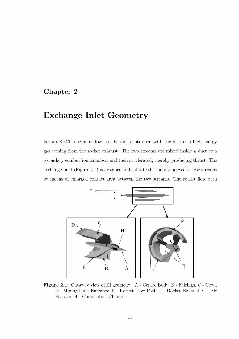
H
Figure 2.1: Cutaway view of EI geometry: A - Centre Body, B - Fairings, C - Cowl,D - Mixing Duct Entrance, E - Rocket Flow Path, F - Rocket Exhaust, G - AirPassage, H - Combustion Chamber.
15
16
(E) is used to expand the flow of hot gases from the combustion chamber (H) into the
mixing duct (D) where it is mixed with the air entrained through the air passage (G)
of the inlet. The shape of the rocket flow path is driven by the desire to increase the
interaction between the air and the rocket exhaust using annular exhaust profile (F),
while reducing the number of pumps and the complexity associated with multiple
combustion chambers. The result is a rocket flow path which diverts the rocket
exhaust from a single combustion chamber into a circular stream of hot gas. The
exchange inlet geometry shown in Figure 2.1 was initially analysed for subsonic flight
conditions only [20], [22]. The blunt shapes of the leading edges of the cowl (C) and the
fairings (B) are not well suited for supersonic flight conditions. Even though this is the
case this geometry is still used to demonstrate how the high losses are estimated, since
the geometry generates all of the shocks expected over the exchange inlet, including
those that would be detached even for a sharper geometry. The detailed design
procedures for this geometry are described by T. Waung in his thesis [20] and are
not repeated here. The EI geometry used in this work is taken directly from T.
Waung results and as such is not currently optimized for any flight profile. Due to
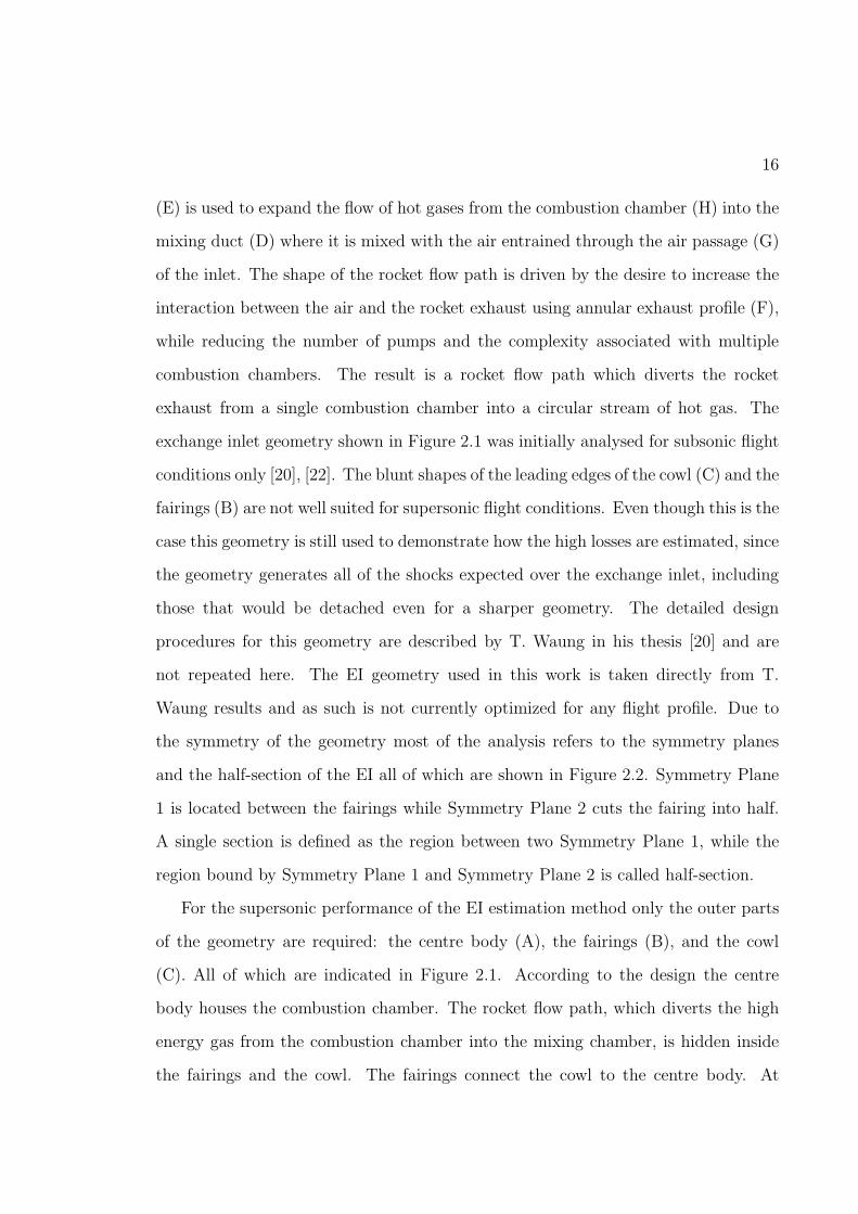
the symmetry of the geometry most of the analysis refers to the symmetry planes
and the half-section of the EI all of which are shown in Figure 2.2. Symmetry Plane
1 is located between the fairings while Symmetry Plane 2 cuts the fairing into half.
A single section is defined as the region between two Symmetry Plane 1, while the
region bound by Symmetry Plane 1 and Symmetry Plane 2 is called half-section.
For the supersonic performance of the EI estimation method only the outer parts
of the geometry are required: the centre body (A), the fairings (B), and the cowl
(C). All of which are indicated in Figure 2.1. According to the design the centre
body houses the combustion chamber. The rocket flow path, which diverts the high
energy gas from the combustion chamber into the mixing chamber, is hidden inside
the fairings and the cowl. The fairings connect the cowl to the centre body. At
17
SymmetryPlane 2
SymmetryPlane 1
Half-sectionof EI
Sectionof EI
SymmetryPlane 1
Figure 2.2: Definition of half-section of the EI and the symmetry planes.
supersonic speeds all of the outer geometries produce shocks. These shocks will be
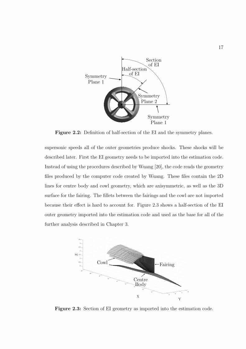
described later. First the EI geometry needs to be imported into the estimation code.
Instead of using the procedures described by Wuang [20], the code reads the geometry
files produced by the computer code created by Wuang. These files contain the 2D
lines for centre body and cowl geometry, which are axisymmetric, as well as the 3D
surface for the fairing. The fillets between the fairings and the cowl are not imported
because their effect is hard to account for. Figure 2.3 shows a half-section of the EI
outer geometry imported into the estimation code and used as the base for all of the
further analysis described in Chapter 3.
−4
−2
0
2
4
6
8
10
12
01
23
0
0.5
1
1.5
2
2.5
3
3.5
CentreBody
FairingCowl
XY
Z
Figure 2.3: Section of EI geometry as imported into the estimation code.
Chapter 3
Estimation Method
3.1 Overview
The estimation method described within this chapter is designed for fast estimations
of the Exchange Inlet (EI) performance at supersonic flight conditions to select a
viable geometry for further analysis. The method is not meant to provide an exact
solution to the flow and is not as accurate as finite volume CFD computations, how-
ever, it is considerably faster and provides a reasonable estimate for the total pressure
loss due to shocks across the EI. The estimation method is written using MATLAB
software [31] and utilizes some of the MATLAB inner functions such as numerical
ordinary differential equation (ODE) solver and interpolation algorithms.
The EI has three main components that generate shocks: cowl, fairings and the
centre body (Figure 2.1). The shock from the centre body is approximated using a
cone shock solution, while the shocks due to the other two components are approx-
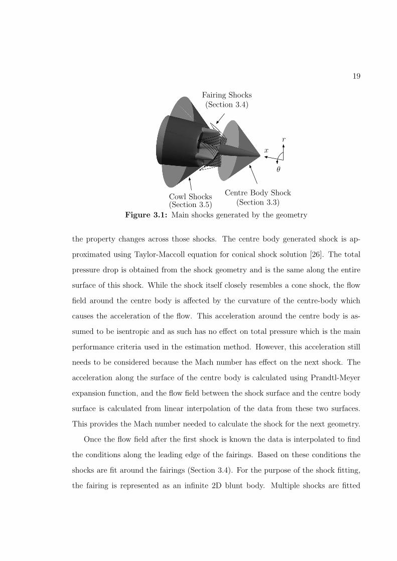
imated using a detached 2D shock solution. Figure 3.1 shows the shocks generated
around the EI. As seen from the figure, the centre body shock is a cone, while the
other two shocks are somewhat more elaborate.
The estimation method is built around determining the shock shapes and finding
18
19
Centre Body Shock(Section 3.3)
Fairing Shocks(Section 3.4)
Cowl Shocks(Section 3.5)
θ
r
x
Figure 3.1: Main shocks generated by the geometry
the property changes across those shocks. The centre body generated shock is ap-
proximated using Taylor-Maccoll equation for conical shock solution [26]. The total
pressure drop is obtained from the shock geometry and is the same along the entire
surface of this shock. While the shock itself closely resembles a cone shock, the flow
field around the centre body is affected by the curvature of the centre-body which
causes the acceleration of the flow. This acceleration around the centre body is as-
sumed to be isentropic and as such has no effect on total pressure which is the main
performance criteria used in the estimation method. However, this acceleration still
needs to be considered because the Mach number has effect on the next shock. The
acceleration along the surface of the centre body is calculated using Prandtl-Meyer
expansion function, and the flow field between the shock surface and the centre body
surface is calculated from linear interpolation of the data from these two surfaces.
This provides the Mach number needed to calculate the shock for the next geometry.
Once the flow field after the first shock is known the data is interpolated to find
the conditions along the leading edge of the fairings. Based on these conditions the
shocks are fit around the fairings (Section 3.4). For the purpose of the shock fitting,
the fairing is represented as an infinite 2D blunt body. Multiple shocks are fitted
20
along the leading edge of the fairing at different radii. This takes into account slight
variations in the geometry of the leading edge of the fairing as well as the difference
in the length of the shocks at different radii. This results in 3D shock-surface. The
flow field from the previous step is projected onto this shock surface and property
changes across the shock are calculated using equations described in Sections 3.2 and
3.4. The total pressure drop across this shock is averaged along the shock surface in
the direction normal to the plane of the leading edge of the fairing. This results in a
radial variation in total pressure, which is then projected onto the cowl shock (which
assumes isentropic flow without any total pressure losses between the two shocks).
The Mach number in this region is changing considerably due to the curvature of the
fairing and the centre body. To take into account the change in Mach number certain
assumptions are made to calculate the flow field between the fairing and the cowl
shocks. These assumptions are described in more detail in Section 3.4.
The cowl is assumed to be an infinite 2D blunt object similar to the fairings. This
allows for a relatively simple curve fit for the shock geometry. Once the shape of this
shock is found, the calculated flow field from the previous shocks are interpolated to
obtain the properties of the flow entering the cowl shock. This shock is then adjusted
for a Mach stem, if one exists, which is calculated from the shape of the EI and the
flow properties behind the cowl shock. Using this new shock shape the flow properties
after the shock are adjusted to take into account the new shock geometry. After that
the properties are averaged in radial direction and the total pressure drop across the
EI is found. Section 3.5 describes this process in more details. In addition to the total
pressure at the exit of the EI, the mass flow rate through the inlet is also computed
(Section 3.6).
21
3.2 Isentropic compressible flow and oblique shock
equations
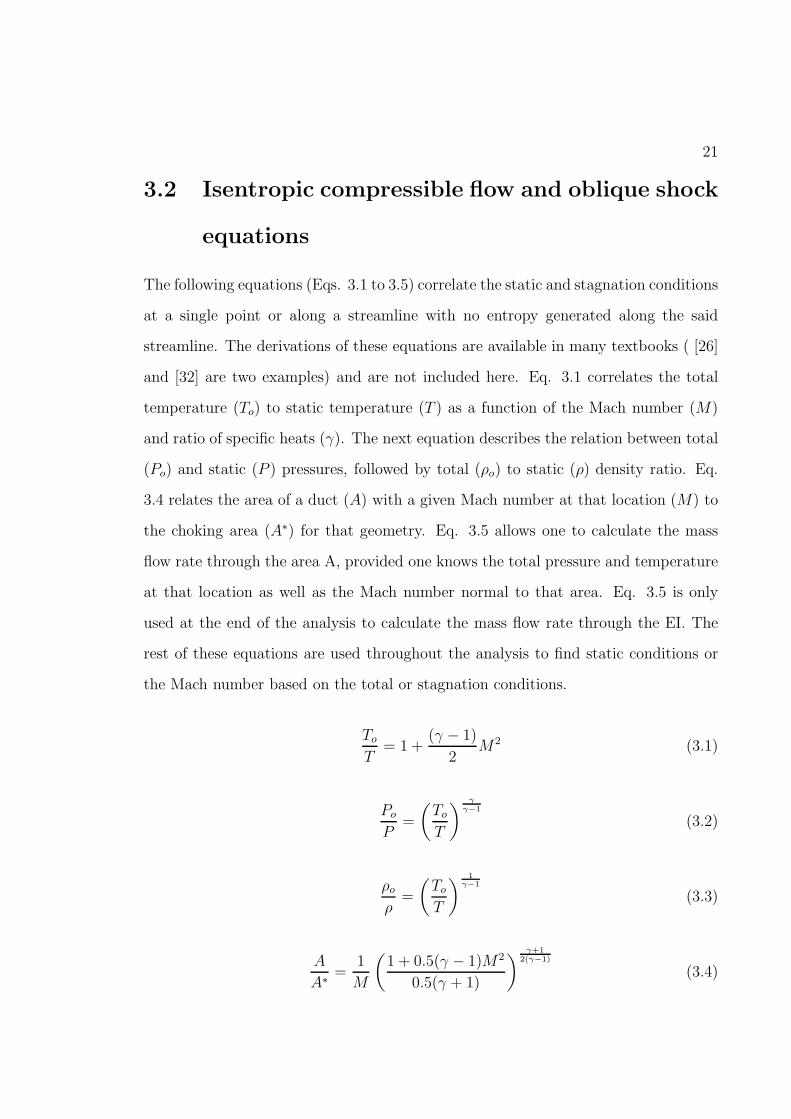
The following equations (Eqs. 3.1 to 3.5) correlate the static and stagnation conditions
at a single point or along a streamline with no entropy generated along the said
streamline. The derivations of these equations are available in many textbooks ( [26]
and [32] are two examples) and are not included here. Eq. 3.1 correlates the total
temperature (To) to static temperature (T ) as a function of the Mach number (M)
and ratio of specific heats (γ). The next equation describes the relation between total
(Po) and static (P ) pressures, followed by total (ρo) to static (ρ) density ratio. Eq.
3.4 relates the area of a duct (A) with a given Mach number at that location (M) to
the choking area (A∗) for that geometry. Eq. 3.5 allows one to calculate the mass
flow rate through the area A, provided one knows the total pressure and temperature
at that location as well as the Mach number normal to that area. Eq. 3.5 is only
used at the end of the analysis to calculate the mass flow rate through the EI. The
rest of these equations are used throughout the analysis to find static conditions or
the Mach number based on the total or stagnation conditions.
ToT
= 1 +(γ − 1)
2M2 (3.1)
PoP
=
(
ToT
)γ
γ−1
(3.2)
ρoρ
=
(
ToT
)1
γ−1
(3.3)
A
A∗=
1
M
(
1 + 0.5(γ − 1)M2
0.5(γ + 1)
)
γ+12(γ−1)
(3.4)
22
m =MAPo
√
γ
RairTo
(
2
2 + (γ − 1)M2
)γ+1
2(γ−1)
(3.5)
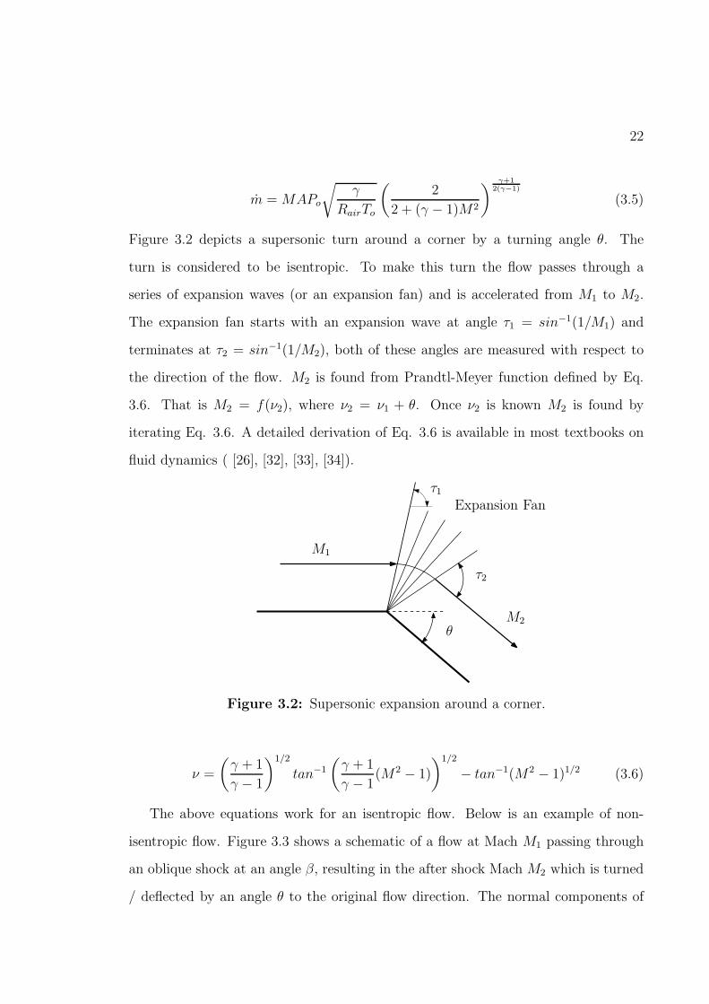
Figure 3.2 depicts a supersonic turn around a corner by a turning angle θ. The
turn is considered to be isentropic. To make this turn the flow passes through a
series of expansion waves (or an expansion fan) and is accelerated from M1 to M2.
The expansion fan starts with an expansion wave at angle τ1 = sin−1(1/M1) and
terminates at τ2 = sin−1(1/M2), both of these angles are measured with respect to
the direction of the flow. M2 is found from Prandtl-Meyer function defined by Eq.
3.6. That is M2 = f(ν2), where ν2 = ν1 + θ. Once ν2 is known M2 is found by
iterating Eq. 3.6. A detailed derivation of Eq. 3.6 is available in most textbooks on
fluid dynamics ( [26], [32], [33], [34]).
M1
M2
θ
Expansion Fanτ1
τ2
Figure 3.2: Supersonic expansion around a corner.
ν =
(
γ + 1
γ − 1
)1/2
tan−1
(
γ + 1
γ − 1(M2 − 1)
)1/2
− tan−1(M2 − 1)1/2 (3.6)
The above equations work for an isentropic flow. Below is an example of non-
isentropic flow. Figure 3.3 shows a schematic of a flow at Mach M1 passing through
an oblique shock at an angle β, resulting in the after shock Mach M2 which is turned
/ deflected by an angle θ to the original flow direction. The normal components of
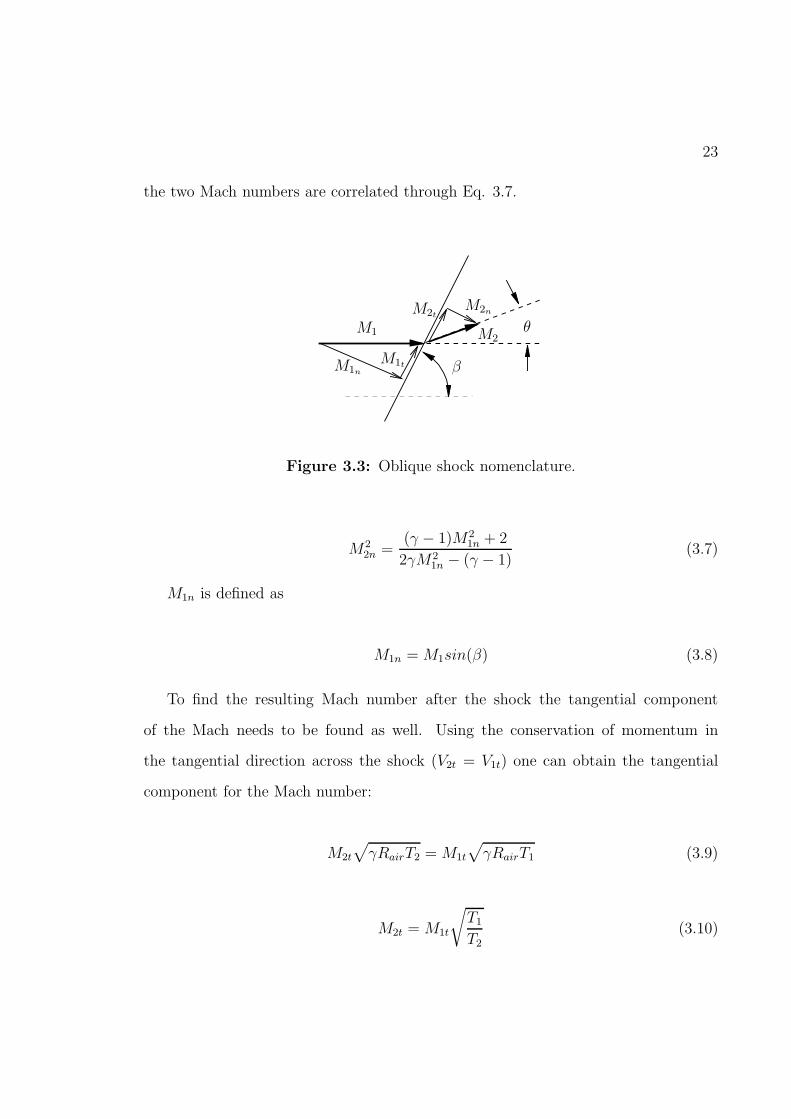
23
the two Mach numbers are correlated through Eq. 3.7.
M1
M1n
M1t
M2tM2n
M2
β
θ
Figure 3.3: Oblique shock nomenclature.
M2
2n =(γ − 1)M2
1n + 2
2γM21n − (γ − 1)
(3.7)
M1n is defined as
M1n =M1sin(β) (3.8)
To find the resulting Mach number after the shock the tangential component
of the Mach needs to be found as well. Using the conservation of momentum in
the tangential direction across the shock (V2t = V1t) one can obtain the tangential
component for the Mach number:
M2t
√
γRairT2 =M1t
√
γRairT1 (3.9)
M2t =M1t
√
T1T2
(3.10)
24
The resulting M2 is calculated from Eq. 3.11 below:
M22 =M2
2t +M22n (3.11)
The following equations (Eqs. 3.12 to 3.16) relate conditions after the shock to
those before the shock.
P12 =P2
P1
=2γM2
1n − (γ − 1)
γ + 1(3.12)
ρ12 =ρ2ρ1
=(γ + 1)M2
1n
(γ − 1)M21n + 2
=P1M
21n
P2M22n
(3.13)
V12 =V2nV1n
=ρ1ρ2
(3.14)
T12 =T2T1
=P2
P1
ρ1ρ2
=P 22M
22n
P 21M
21n
(3.15)
Po12 =Po2Po1
=
(
ρ2ρ1
)γ
γ−1(
P1
P2
)1
γ−1
=
(
M21n
M22n
)
γ
γ−1(
P1
P2
)γ+1γ−1
(3.16)
The notation with two numbers in the subscript indicates the ratio between the
two regions. For example P12 in Eq. 3.12 indicates the pressure ratio for the flow
going from region 1 to region 2.
Based on the above equations it is possible to correlate the deflection of the flow
(θ) with the shock angle (β) and the upstream Mach number (M1):
tan(θ) =2cot(β) (M2
1n − 1)
M21 (γ + cos(2β)) + 2
(3.17)
All of the above equations are essential to calculating the properties of the flow
25
around the EI geometry and provide the backbone for the analysis and the theory
below.
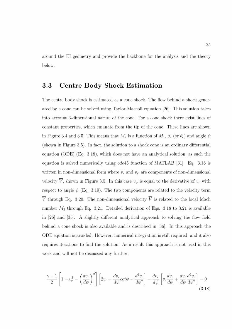
3.3 Centre Body Shock Estimation
The centre body shock is estimated as a cone shock. The flow behind a shock gener-
ated by a cone can be solved using Taylor-Maccoll equation [26]. This solution takes
into account 3-dimensional nature of the cone. For a cone shock there exist lines of
constant properties, which emanate from the tip of the cone. These lines are shown
in Figure 3.4 and 3.5. This means that M2 is a function ofM1, βc (or θc) and angle ψ
(shown in Figure 3.5). In fact, the solution to a shock cone is an ordinary differential
equation (ODE) (Eq. 3.18), which does not have an analytical solution, as such the
equation is solved numerically using ode45 function of MATLAB [31]. Eq. 3.18 is
written in non-dimensional form where vr and vψ are components of non-dimensional
velocity V , shown in Figure 3.5. In this case vψ is equal to the derivative of vr with
respect to angle ψ (Eq. 3.19). The two components are related to the velocity term
V through Eq. 3.20. The non-dimensional velocity V is related to the local Mach
number M2 through Eq. 3.21. Detailed derivation of Eqs. 3.18 to 3.21 is available
in [26] and [35]. A slightly different analytical approach to solving the flow field
behind a cone shock is also available and is described in [36]. In this approach the
ODE equation is avoided. However, numerical integration is still required, and it also
requires iterations to find the solution. As a result this approach is not used in this
work and will not be discussed any further.
γ − 1
2
[
1− v2r −
(
dvrdψ
)2]
[
2vr +dvrdψ
cotψ +d2vrdψ2
]
−dvrdψ
[
vrdvrdψ
+dvrdψ
d2vrdψ2
]
= 0
(3.18)
26
M1
M2
θc
βc
Shock
Lines ofconstantproperties
Figure 3.4: Shock generated by a cone at zero angle of attack.
M1V (ψ),M2(ψ)
vr
vψ
ψ
Shock
r
Figure 3.5: Cone shock with non-dimensional velocity components shown.
vψ =dvrdψ
(3.19)
V (ψ)2 = v2r + v2ψ (3.20)
V =
(
2
(γ − 1)M22
+ 1
)
−1/2
(3.21)
Eq. 3.18 is integrated from the shock (βc) to the surface of the cone (θc). The
27
boundary conditions of this integration are dvrdψ
(ψ = θc) = 0 and the flow properties
right after the shock which are found using Eq. 3.7 to 3.17. The fact that Eq. 3.18 is
integrated starting from the shock surface means that the cone surface location or θc is
not known beforehand. However, for the given problem θc is known and βc is what is
needed. This leads to an iterative process of finding the desired βc for the given θc. If
one needs to find the cone solution for different conditions and different geometries, it
might take a considerable amount of time to perform the numerical integration while
continuously iterating. To speed up the calculation process the numerical integration
is performed beforehand and the results for the βc, θc and Mach number at the cone
surface Mc are stored as a function of the free stream Mach number in a database.
Figure 3.6 shows the dependence of the cone shock angle (βc) on both the cone half-
angle (θc) and the free stream Mach number. As seen from the figure for each half
cone angle (θc) there exist two solutions: one corresponding to a weak shock (lower
shock angle), and another one corresponding to strong shock (higher shock angle). In
this work only the weak shock solution is of interest.
0 10 20 30 40 50 600
10
20
30
40
50
60
70
80
90
θc (degrees)
βc(degrees)
M = 1.1M = 2.0M = 3.0M = 5.0M = 10M = 100
Figure 3.6: Cone shock angle dependence on the cone half-angle and the free streamMach number.
The above describes the solution of the flow past a shock generated by a cone
of infinite length. However, the surface of the centre-body is curved (as can be
28
seen from Figure 2.1), this leads to acceleration of the flow along the surface of the
centre body. The acceleration of the flow can be calculated by using Prandtl-Meyer
expansion by starting at the tip of the centre body with θ = θc and M = Mc, both
of which are known from cone shock calculations. This yields the Mach distribution
along the surface of the centre body (Mcb in Figure 3.7). At this point the properties
of the flow are known along the surface of the centre body (Mcb(x)) and along the
downstream surface of the shock generated by this geometry (Mcs). The flow field
between the object surface and the shock requires additional computations (MFF ).
Assuming isentropic flow in this region for a given axial location both the Mach value
and the direction of the flow are linearly interpolated in the radial direction between
the centre body and the shock surface of the same x-location.
x
r
EI centrelineCentre body surface
Mcb(x)
Centre body shock
Mcs
MFF (x, r) interpolated
from Mcb(x) and Mcs
M∞
Figure 3.7: Schematic of cone shock generated by a centre body.
3.4 Fairings Shock Estimation
Figure 3.8 shows the EI fairings with shocks drawn around them. This is a zoomed
in version of Figure 3.1 without centre body and cowl shocks. The detached bow
shocks (shown) are caused by supersonic flow that comes after the centre body shock
(MFF (x, r)). Before going into detailed analysis of the detached bow shock, a simple
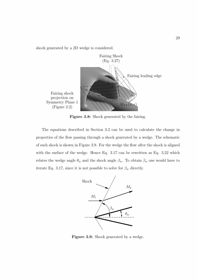
29
shock generated by a 2D wedge is considered.
Fairing Shock(Eq. 3.27)
Fairing shockprojection on
Symmetry Plane 1(Figure 2.2)
MFF (x, r)
Fairing leading edge
Figure 3.8: Shock generated by the fairing.
The equations described in Section 3.2 can be used to calculate the change in
properties of the flow passing through a shock generated by a wedge. The schematic
of such shock is shown in Figure 3.9. For the wedge the flow after the shock is aligned
with the surface of the wedge. Hence Eq. 3.17 can be rewritten as Eq. 3.22 which
relates the wedge angle θw and the shock angle βw. To obtain βw one would have to
iterate Eq. 3.17, since it is not possible to solve for βw directly.
M1
M2
θw
βw
Shock
Figure 3.9: Shock generated by a wedge.
30
tan(θw) =2cot(βw) (M
21n − 1)
M21 (γ + cos(2βw)) + 2
(3.22)
By differentiating Eq. 3.22 with respect to βw one can obtain the shock angle at
which the maximum deflection of the flow can be obtained at a given Mach number
(Eq. 3.23) for which the shock is still attached. By substituting βθd into Eq. 3.17 one
can obtain the maximum deflection angle (θd).
βθd = sin−1
(
γ + 1
4γM2
{
M2 −4
γ + 1+
[
M4 + 8
(
γ − 1
γ + 1
)
M2 +16
γ + 1
]1/2})1/2
(3.23)
If the wedge angle θw is larger than θd then the flow detaches from the wedge and
a strong shock is formed. This situation looks similar to the one shown in Figure
3.10. An analytical solution to the detached shock is not available, however, there
are other various approaches to solving for the shape of the detached shocks. Many of
these involve the numerical solution of Euler’s equations in one form or another. One
of the examples includes a moving boundary method in which a mesh boundary is
set as the shock and the location of that boundary is found through iterations, while
at the same time solving for the flow field between the shock and the blunt object.
One such method is described in [30]. A more general Finite Volume Method (FVM)
is another example [37]. However, both of the above examples require considerable
amount of computation resources to produce reasonable results, especially the FVM
(used by Ansys-CFX), as they solve for the entire flow field after the shock. To
keep the calculation time as short as possible a curve fit solution to the shape of the
detached shock is used. Once the shape of the shock is known it is possible to find the
flow properties right behind the shock using the equations described in the previous
sections (Eqs. 3.7 to 3.17).
31
βw
θwRs
Rds
Asymptote ofHyperbola
aaǫ
Focus of Hyperbola
Eq. 3.27
x
y
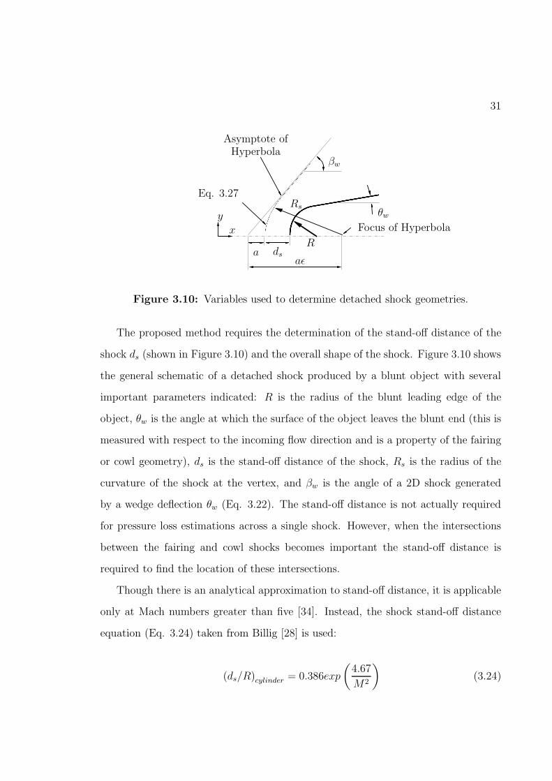
Figure 3.10: Variables used to determine detached shock geometries.
The proposed method requires the determination of the stand-off distance of the
shock ds (shown in Figure 3.10) and the overall shape of the shock. Figure 3.10 shows
the general schematic of a detached shock produced by a blunt object with several
important parameters indicated: R is the radius of the blunt leading edge of the
object, θw is the angle at which the surface of the object leaves the blunt end (this is
measured with respect to the incoming flow direction and is a property of the fairing
or cowl geometry), ds is the stand-off distance of the shock, Rs is the radius of the
curvature of the shock at the vertex, and βw is the angle of a 2D shock generated
by a wedge deflection θw (Eq. 3.22). The stand-off distance is not actually required
for pressure loss estimations across a single shock. However, when the intersections
between the fairing and cowl shocks becomes important the stand-off distance is
required to find the location of these intersections.
Though there is an analytical approximation to stand-off distance, it is applicable
only at Mach numbers greater than five [34]. Instead, the shock stand-off distance
equation (Eq. 3.24) taken from Billig [28] is used:
(ds/R)cylinder = 0.386exp
(
4.67
M2
)
(3.24)
32
Since R is a property of the geometry (either fairing or cowl) it is known which
allows ds to be found for a given Mach number.
With the values of R and βw determined it is possible to use a hyperbolic profile
of the following form [28]
x = R + ds −Rscot2(βw)
[√
(
1 +y2tan2(βw)
R2s
)
− 1
]
(3.25)
to represent the shock shape (the origin is set at the center of the body curvature R).
The variable Rs is the radius of curvature of the shock, which for a cylinder according
to Billig [28] is found from
(Rs/R)cylinder = 1.386exp
(
1.8
(M − 1)0.75
)
(3.26)
For higher Mach numbers these equations provide good estimates for the shock
shape in the immediate proximity to the blunt body. However, at distances further
away from the body and at lower Mach numbers these approximations decrease in
accuracy. The difference between the shock profile described by Billig (Eqs. 3.25 and
3.26) and the CFD simulations are discussed in Section 4.4 in more detail. Due to
these differences a slightly modified procedure is used.
A hyperbola-like shock shape is still maintained using Eq. 3.27 with n parameter
set to 1.7. xo is the location of the leading edge of the object. The value of ds is found
using Eq. 3.24. Parameters a and b are related to the shock angle βw through Eq.
3.28. The value of βw is found from Eq. 3.22 based on the known deflection angle θw
(obtained from geometry) and the upstream Mach number. The value of a is found
from Eq. 3.29, where ǫ is defined by Eq. 3.30 and Rs is estimated based on Eq. 3.31.
Eq. 3.31 is based on curve-fit of the shock from 2D CFD simulations described in
Chapter 4.
33
(x− xo + a+ ds)n
an−yn
bn= 1 (3.27)
b
a= tan(βw) (3.28)
a =Rs
ǫ− 1(3.29)
ǫ =√
1 + tan2(βw) (3.30)
Rs/R = 0.1589exp
(
6.3366
M
)
+ 1.9187 (3.31)
This approximation provides slightly better results especially at lower Mach num-
bers (M∞ < 2.0). Once the shock shape has been determined it can be applied to the
leading edge of either fairing or cowl and the changes in properties across the shocks
can be easily calculated using the equations for a 2D oblique shock.
Figure 3.11 shows a cut of the EI geometry with the example of the shock plane
and the shock geometry. The calculations described above are performed for a number
of shock planes located at different radii along the leading edge of the fairing. The
exact number of shock planes is set by the user. The shock geometry is calculated
based on the normal component of the Mach number along the leading edge of the
fairing which is interpolated from the flow field calculated in Section 3.3. Once the
shape of the shock is known the projection of the Mach number onto the shock plane
(Mxy) is again interpolated from the previously calculated flow field. The property
changes across the shock are calculated from Eqs. 3.7 to 3.16 using local value of
the shock angle β along the shock line. Should the cone shock intersect the leading
edge of the fairing or the fairing shock then the free stream conditions are used above
34
the location of the intersection. The process is repeated for all of the shock planes
resulting in a 3D surface for the fairing shock with all parameters known. At this
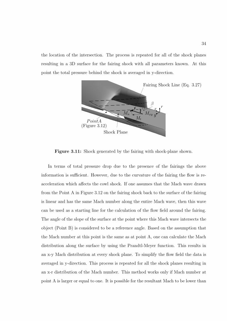
point the total pressure behind the shock is averaged in y-direction.
Fairing Shock Line (Eq. 3.27)
Mxy
β
Shock Plane
Mn
MtPointA
(Figure 3.12)
rx
y
Figure 3.11: Shock generated by the fairing with shock-plane shown.
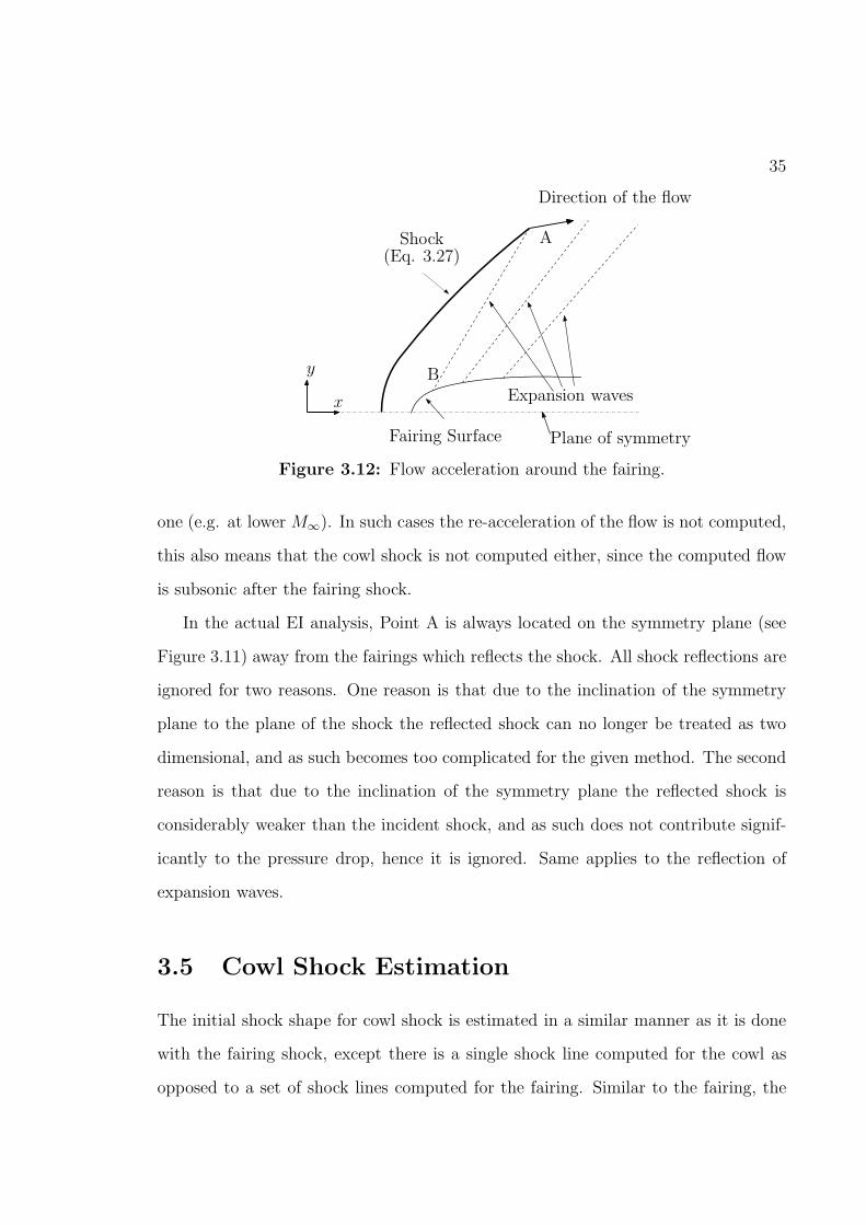
In terms of total pressure drop due to the presence of the fairings the above
information is sufficient. However, due to the curvature of the fairing the flow is re-
acceleration which affects the cowl shock. If one assumes that the Mach wave drawn
from the Point A in Figure 3.12 on the fairing shock back to the surface of the fairing
is linear and has the same Mach number along the entire Mach wave, then this wave
can be used as a starting line for the calculation of the flow field around the fairing.
The angle of the slope of the surface at the point where this Mach wave intersects the
object (Point B) is considered to be a reference angle. Based on the assumption that
the Mach number at this point is the same as at point A, one can calculate the Mach
distribution along the surface by using the Prandtl-Meyer function. This results in
an x-y Mach distribution at every shock plane. To simplify the flow field the data is
averaged in y-direction. This process is repeated for all the shock planes resulting in
an x-r distribution of the Mach number. This method works only if Mach number at
point A is larger or equal to one. It is possible for the resultant Mach to be lower than
35
Shock(Eq. 3.27)
Fairing Surface
Expansion waves
Direction of the flow
B
A
Plane of symmetry
x
y
Figure 3.12: Flow acceleration around the fairing.
one (e.g. at lower M∞). In such cases the re-acceleration of the flow is not computed,
this also means that the cowl shock is not computed either, since the computed flow
is subsonic after the fairing shock.
In the actual EI analysis, Point A is always located on the symmetry plane (see
Figure 3.11) away from the fairings which reflects the shock. All shock reflections are
ignored for two reasons. One reason is that due to the inclination of the symmetry
plane to the plane of the shock the reflected shock can no longer be treated as two
dimensional, and as such becomes too complicated for the given method. The second
reason is that due to the inclination of the symmetry plane the reflected shock is
considerably weaker than the incident shock, and as such does not contribute signif-
icantly to the pressure drop, hence it is ignored. Same applies to the reflection of
expansion waves.
3.5 Cowl Shock Estimation
The initial shock shape for cowl shock is estimated in a similar manner as it is done
with the fairing shock, except there is a single shock line computed for the cowl as
opposed to a set of shock lines computed for the fairing. Similar to the fairing, the
36
cowl shock geometry is based on the flow condition interpolated from the flow field at
the leading edge of the cowl. The formulation of the generated detached shock is the
same as in the case of the fairing, that is Eqs. 3.24 and 3.27 to 3.31 are used. The
complication for the cowl shock comes from the Mach stem, which cannot be ignored.
Below is a short introduction of the reflected shock, which needs to be understood
before analysing the Mach stem.
In the cases where a supersonic flow remains supersonic after passing through
a shock and encounters a surface, the flow would have to make a turn by passing
through another shock. Figure 3.13a shows a schematic of this situation. In this case
the fluid is moving at Mach M1 before encountering the first shock. After passing the
first shock the new Mach number is M2, which in this case is above one. The flow
is now moving at angle θr with respect to the surface, which means it has to turn
by that angle to be aligned with the surface again. Since at this point the flow is
supersonic, to make this turn it has to pass through another shock (reflected shock).
The situation where θr is lower than the maximum deflection angle θd is called a
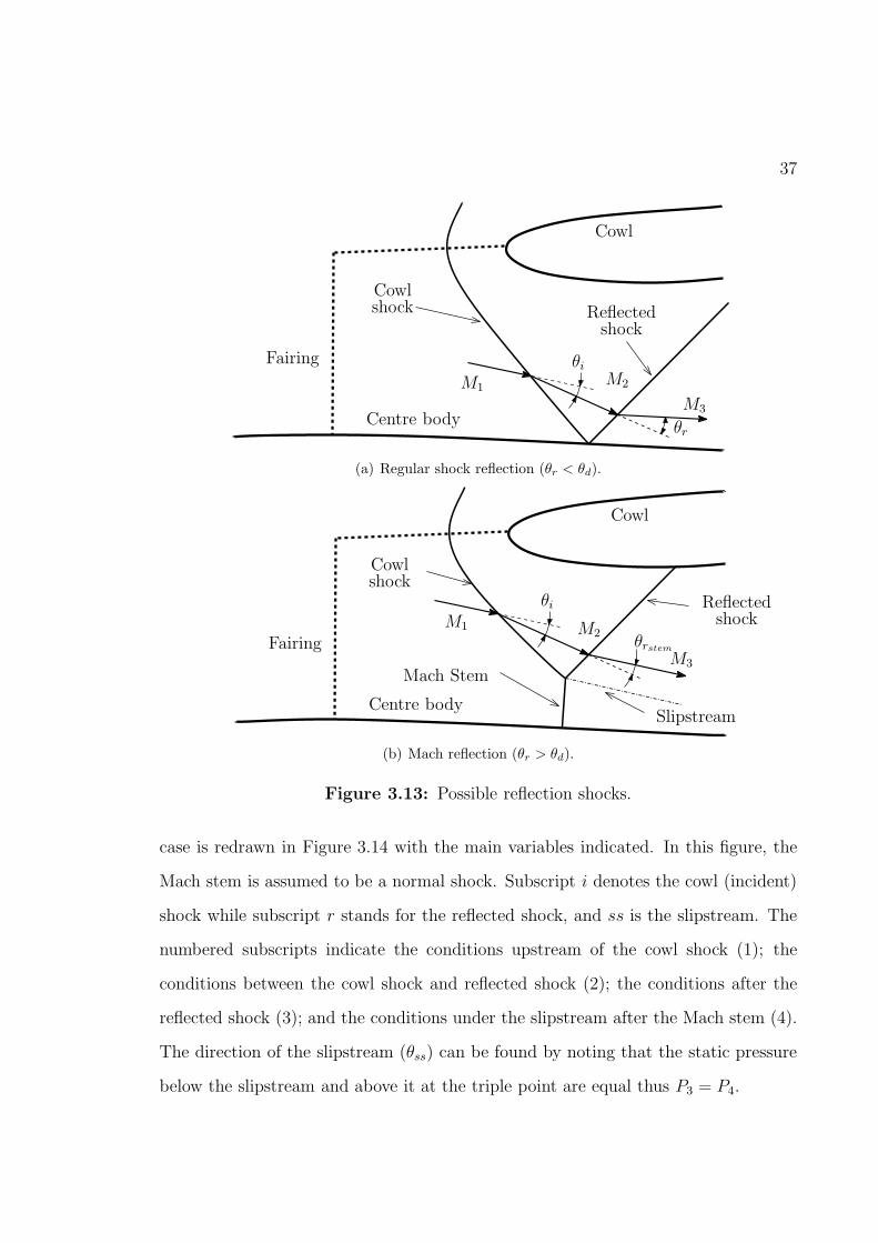
regular reflection and the flow behaves as shown in Figure 3.13a.
In cases where θr is larger than the maximum deflection angle θd the flow can
no longer be turned sufficiently using an attached shock and instead a strong shock,
called a Mach stem, is generated at the surface. This situation is shown in Figure
3.13b. The flow passing through the Mach stem becomes subsonic, while above the
Mach stem the flow is either subsonic or supersonic and passes through a weak oblique
shock (reflection shock). The resulting θrstem is lower than θd and the flow above the
slipstream is moving at an angle towards the surface.
The size of the Mach stem depends on the downstream conditions. Ben-Dor [38]
describes a method to calculate the size of the Mach stem which works for a finite
wedge geometry and a known back pressure. To use this method one first requires the
direction of the flow after the reflected shock (θss). A close up of the Mach reflection
37PSfrag
Centre body
Fairing
Cowl
M1M2
M3
Cowlshock Reflected
shock
θi
θr
(a) Regular shock reflection (θr < θd).
Centre body
Fairing
Cowl
Cowlshock
M1 M2
M3
Reflectedshock
θi
θrstem
Mach Stem
Slipstream
(b) Mach reflection (θr > θd).
Figure 3.13: Possible reflection shocks.
case is redrawn in Figure 3.14 with the main variables indicated. In this figure, the
Mach stem is assumed to be a normal shock. Subscript i denotes the cowl (incident)
shock while subscript r stands for the reflected shock, and ss is the slipstream. The
numbered subscripts indicate the conditions upstream of the cowl shock (1); the
conditions between the cowl shock and reflected shock (2); the conditions after the
reflected shock (3); and the conditions under the slipstream after the Mach stem (4).
The direction of the slipstream (θss) can be found by noting that the static pressure
below the slipstream and above it at the triple point are equal thus P3 = P4.
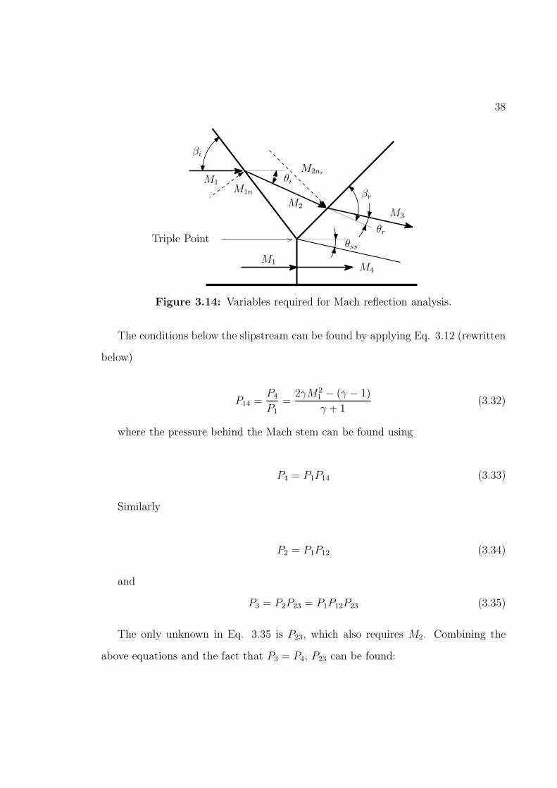
38
M1
M1
M1n
βi
M2nr
M2
M3
θi
θrθss
M4
βr
Triple Point
Figure 3.14: Variables required for Mach reflection analysis.
The conditions below the slipstream can be found by applying Eq. 3.12 (rewritten
below)
P14 =P4
P1
=2γM2
1 − (γ − 1)
γ + 1(3.32)
where the pressure behind the Mach stem can be found using
P4 = P1P14 (3.33)
Similarly
P2 = P1P12 (3.34)
and
P3 = P2P23 = P1P12P23 (3.35)
The only unknown in Eq. 3.35 is P23, which also requires M2. Combining the
above equations and the fact that P3 = P4, P23 can be found:
39
P23 =P14
P12
=2γM2
1 − (γ − 1)
2γM21n − (γ − 1)
(3.36)
where M1n = M1sin(βi), which is found from the fitted solution for the cowl
shock. On the other hand P23 is defined as
P23 =2γM2
2nr− (γ − 1)
γ + 1(3.37)
where M2nr= M2sin(βr). The subscript r in this case indicates that the nor-
mal component is with respect to the reflected shock. By combining the above two
equations one can find M2nr:
M2nr=
([
2γM21 − (γ − 1)
2γM21n − (γ − 1)
(γ + 1) + (γ − 1)
]
1
2γ
)1/2
(3.38)
βr = sin−1(M2nr/M2) (3.39)
While M2 can be found by following procedures for an oblique shock as outlined
in Section 3.2 (Eqs. 3.7, 3.10 to 3.12 and 3.15).
With M2 and M2nrknown, θr can be found using Eq. 3.17:
tan(θr) =2cot(βr)M
22nr
− 1
M22 (γ + cos(2βr)) + 2
(3.40)
The angle of the slipstream is then the difference between the θi and θr (Eq. 3.41),
while the conditions at 3 are completely defined once the conditions at 2 have been
found (Figure 3.14).
θss = θi − θr (3.41)
If one assumes that the flow passing through the Mach stem is going to choke
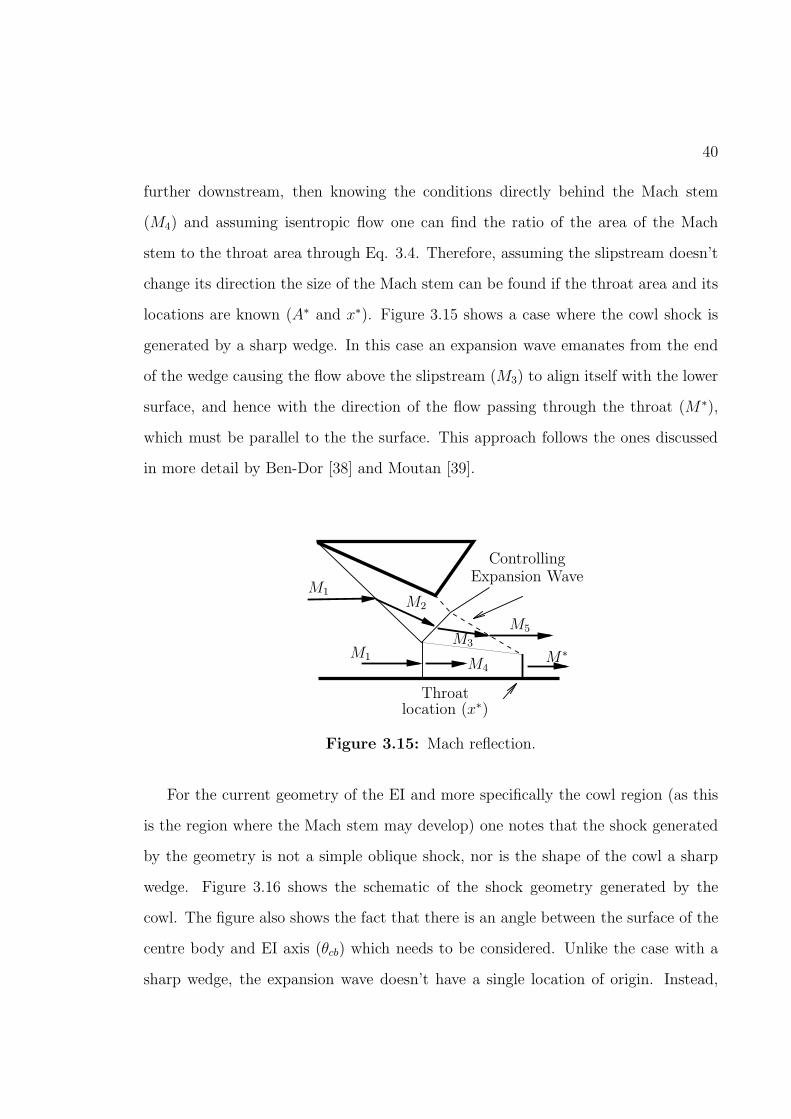
40
further downstream, then knowing the conditions directly behind the Mach stem
(M4) and assuming isentropic flow one can find the ratio of the area of the Mach
stem to the throat area through Eq. 3.4. Therefore, assuming the slipstream doesn’t
change its direction the size of the Mach stem can be found if the throat area and its
locations are known (A∗ and x∗). Figure 3.15 shows a case where the cowl shock is
generated by a sharp wedge. In this case an expansion wave emanates from the end
of the wedge causing the flow above the slipstream (M3) to align itself with the lower
surface, and hence with the direction of the flow passing through the throat (M∗),
which must be parallel to the the surface. This approach follows the ones discussed
in more detail by Ben-Dor [38] and Moutan [39].
M1
M1
M2
M3
M4
M5
M∗
ControllingExpansion Wave
Throatlocation (x∗)
Figure 3.15: Mach reflection.
For the current geometry of the EI and more specifically the cowl region (as this
is the region where the Mach stem may develop) one notes that the shock generated
by the geometry is not a simple oblique shock, nor is the shape of the cowl a sharp
wedge. Figure 3.16 shows the schematic of the shock geometry generated by the
cowl. The figure also shows the fact that there is an angle between the surface of the
centre body and EI axis (θcb) which needs to be considered. Unlike the case with a
sharp wedge, the expansion wave doesn’t have a single location of origin. Instead,
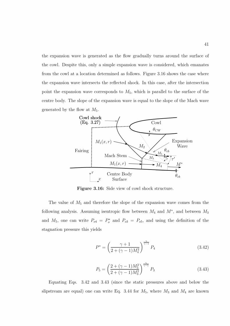
41
the expansion wave is generated as the flow gradually turns around the surface of
the cowl. Despite this, only a simple expansion wave is considered, which emanates
from the cowl at a location determined as follows. Figure 3.16 shows the case where
the expansion wave intersects the reflected shock. In this case, after the intersection
point the expansion wave corresponds to M5, which is parallel to the surface of the
centre body. The slope of the expansion wave is equal to the slope of the Mach wave
generated by the flow at M5.
Centre BodySurface
Fairing
CowlCowl shock(Eq. 3.27)Cowl shock(Eq. 3.27)
M1(x, r)
θCW
M3
ExpansionWaveM2
M5Mach Stem
M1(x, r) M4M∗
θcb
θcb
τ τ ′
x
r
Figure 3.16: Side view of cowl shock structure.
The value of M5 and therefore the slope of the expansion wave comes from the
following analysis. Assuming isentropic flow between M4 and M∗, and between M3
and M5, one can write Po4 = P ∗
o and Po3 = Po5, and using the definition of the
stagnation pressure this yields
P ∗ =
(
γ + 1
2 + (γ − 1)M24
)γ
γ−1
P4 (3.42)
P5 =
(
2 + (γ − 1)M25
2 + (γ − 1)M23
)
γγ−1
P3 (3.43)
Equating Eqs. 3.42 and 3.43 (since the static pressures above and below the
slipstream are equal) one can write Eq. 3.44 for M5, where M3 and M4 are known
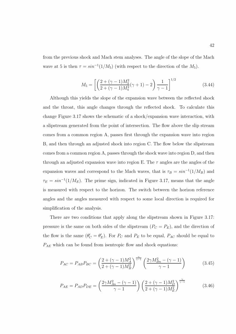
42
from the previous shock and Mach stem analyses. The angle of the slope of the Mach
wave at 5 is then τ = sin−1(1/M5) (with respect to the direction of the M5).
M5 =
[(
2 + (γ − 1)M23
2 + (γ − 1)M24
(γ + 1)− 2
)
1
γ − 1
]1/2
(3.44)
Although this yields the slope of the expansion wave between the reflected shock
and the throat, this angle changes through the reflected shock. To calculate this
change Figure 3.17 shows the schematic of a shock/expansion wave interaction, with
a slipstream generated from the point of intersection. The flow above the slip stream
comes from a common region A, passes first through the expansion wave into region
B, and then through an adjusted shock into region C. The flow below the slipstream
comes from a common region A, passes through the shock wave into region D, and then
through an adjusted expansion wave into region E. The τ angles are the angles of the
expansion waves and correspond to the Mach waves, that is τB = sin−1(1/MB) and
τE = sin−1(1/ME). The prime sign, indicated in Figure 3.17, means that the angle
is measured with respect to the horizon. The switch between the horizon reference
angles and the angles measured with respect to some local direction is required for
simplification of the analysis.
There are two conditions that apply along the slipstream shown in Figure 3.17:
pressure is the same on both sides of the slipstream (PC = PE), and the direction of
the flow is the same (θ′C = θ′E). For PC and PE to be equal, PAC should be equal to
PAE which can be found from isentropic flow and shock equations:
PAC = PABPBC =
(
2 + (γ − 1)M2A
2 + (γ − 1)M2B
)
γγ−1(
2γM2Bn − (γ − 1)
γ − 1
)
(3.45)
PAE = PADPDE =
(
2γM2An − (γ − 1)
γ − 1
)(
2 + (γ − 1)M2D
2 + (γ − 1)M2E
)
γ
γ−1
(3.46)
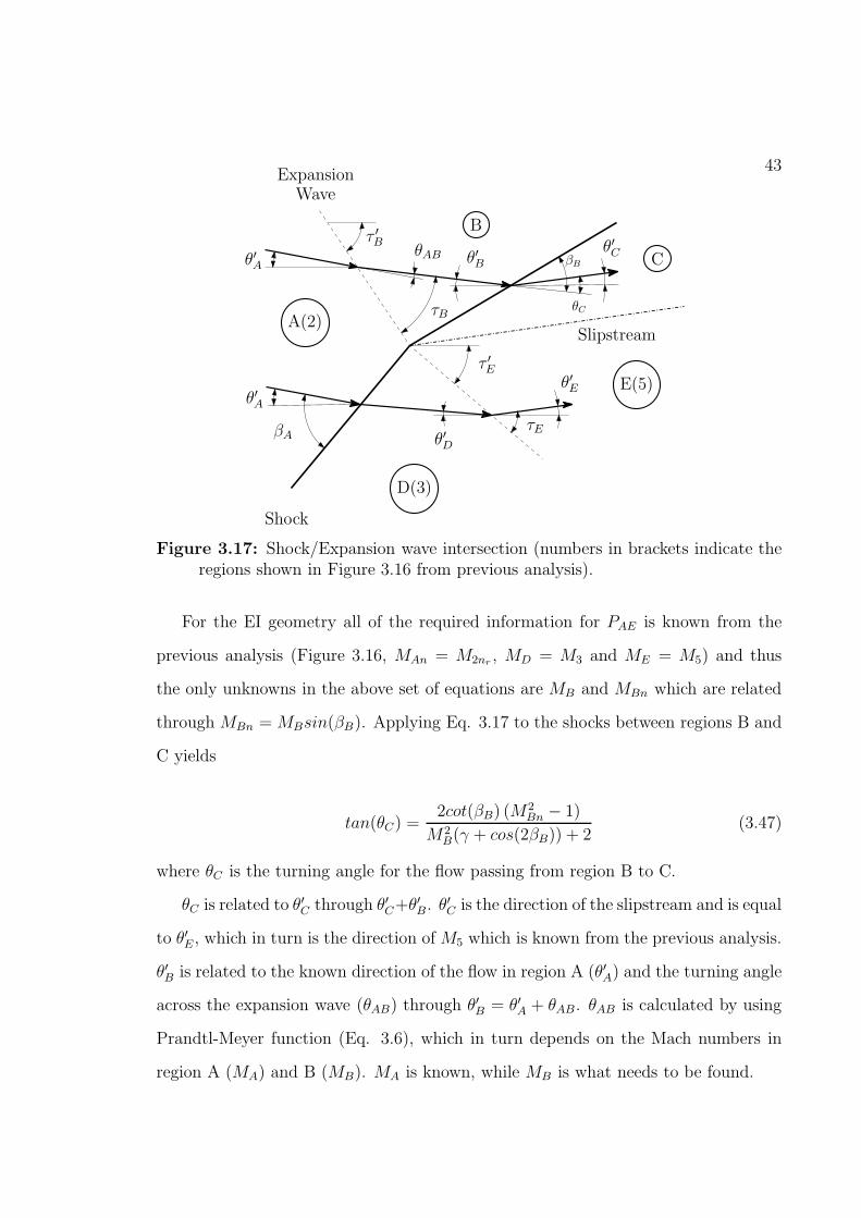
43
A(2)
B
C
D(3)
E(5)
Shock
ExpansionWave
Slipstream
θ′A
θ′A
βA
βB
τB
τ ′B
τE
τ ′E
θ′B
θC
θ′C
θ′D
θ′E
θAB
Figure 3.17: Shock/Expansion wave intersection (numbers in brackets indicate theregions shown in Figure 3.16 from previous analysis).
For the EI geometry all of the required information for PAE is known from the
previous analysis (Figure 3.16, MAn = M2nr, MD = M3 and ME = M5) and thus
the only unknowns in the above set of equations are MB and MBn which are related
through MBn =MBsin(βB). Applying Eq. 3.17 to the shocks between regions B and
C yields
tan(θC) =2cot(βB) (M
2Bn − 1)
M2B(γ + cos(2βB)) + 2
(3.47)
where θC is the turning angle for the flow passing from region B to C.
θC is related to θ′C through θ′C+θ′
B. θ′
C is the direction of the slipstream and is equal
to θ′E , which in turn is the direction ofM5 which is known from the previous analysis.
θ′B is related to the known direction of the flow in region A (θ′A) and the turning angle
across the expansion wave (θAB) through θ′
B = θ′A + θAB. θAB is calculated by using
Prandtl-Meyer function (Eq. 3.6), which in turn depends on the Mach numbers in
region A (MA) and B (MB). MA is known, while MB is what needs to be found.
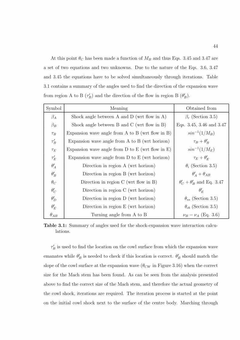
44
At this point θC has been made a function ofMB and thus Eqs. 3.45 and 3.47 are
a set of two equations and two unknowns. Due to the nature of the Eqs. 3.6, 3.47
and 3.45 the equations have to be solved simultaneously through iterations. Table
3.1 contains a summary of the angles used to find the direction of the expansion wave
from region A to B (τ ′B) and the direction of the flow in region B (θ′B).
Symbol Meaning Obtained from
βA Shock angle between A and D (wrt flow in A) βr (Section 3.5)
βB Shock angle between B and C (wrt flow in B) Eqs. 3.45, 3.46 and 3.47
τB Expansion wave angle from A to B (wrt flow in B) sin−1(1/MB)
τ ′B Expansion wave angle from A to B (wrt horizon) τB + θ′B
τE Expansion wave angle from D to E (wrt flow in E) sin−1(1/ME)
τ ′E Expansion wave angle from D to E (wrt horizon) τE + θ′E
θ′A Direction in region A (wrt horizon) θi (Section 3.5)
θ′B Direction in region B (wrt horizon) θ′A + θAB
θC Direction in region C (wrt flow in B) θ′C + θ′B and Eq. 3.47
θ′C Direction in region C (wrt horizon) θ′E
θ′D Direction in region D (wrt horizon) θss (Section 3.5)
θ′E Direction in region E (wrt horizon) θcb (Section 3.5)
θAB Turning angle from A to B νB − νA (Eq. 3.6)
Table 3.1: Summary of angles used for the shock-expansion wave interaction calcu-lations.
τ ′B is used to find the location on the cowl surface from which the expansion wave
emanates while θ′B is needed to check if this location is correct. θ′B should match the
slope of the cowl surface at the expansion wave (θCW in Figure 3.16) when the correct
size for the Mach stem has been found. As can be seen from the analysis presented
above to find the correct size of the Mach stem, and therefore the actual geometry of
the cowl shock, iterations are required. The iteration process is started at the point
on the initial cowl shock next to the surface of the centre body. Marching through
45
the points above it the process is repeated until the correct Mach stem size is found.
The following is a summary of the preceding Mach stem analysis. The initial cowl
shock shape is estimated (Eq. 3.27) based on the Mach number at the leading edge of
the cowl (M1(x, r)) and the flow properties after the shock are calculated. Assuming
the location of the triple point(Figure 3.14) the direction of the slipstream (θss or θ′
D)
and the reflection shock (βr or βA) are obtained. Using the direction of the slipstream
and the properties of the flow right after the Mach stem the location and the size
of the throat are calculated (x∗ and A∗). Using the throat location the direction of
the flow through the throat (θcb or θ′
E) (parallel to the surface of the centre body at
throat location) is obtained, which is used to find the location of intersection of the
reflection shock and the expansion wave emanating back from the throat location.
This information is required to check if the assumed triple point location (i.e. the
height of the Mach stem) is correct. Assuming the shock angle of the reflection shock
between region B and C (βB), the direction of the expansion wave (τB) as well as the
direction of the flow in regions B (θ′B) and C (θ′C) are computed. If the direction of
the flow in region C (θ′C) does not match the direction of the flow in region E (θ′E)
the previous step is repeated with a new value of the shock angle (βB). Once θ′E = θ′C
the direction of the flow in region B (θ′B) is compared to the slope of the cowl at the
point where the expansion wave intersects it (θCW ). If the two match, then the size
of the Mach stem is correct, otherwise, the process for the Mach stem is repeated
with a new location for the triple point. Once a viable location of the triple point is
found, the geometry of the cowl shock as well as the flow properties after the cowl
shock are adjusted to incorporate the effect of the Mach stem. Afterwards the flow
properties after the cowl shock are averaged in the radial direction for output.
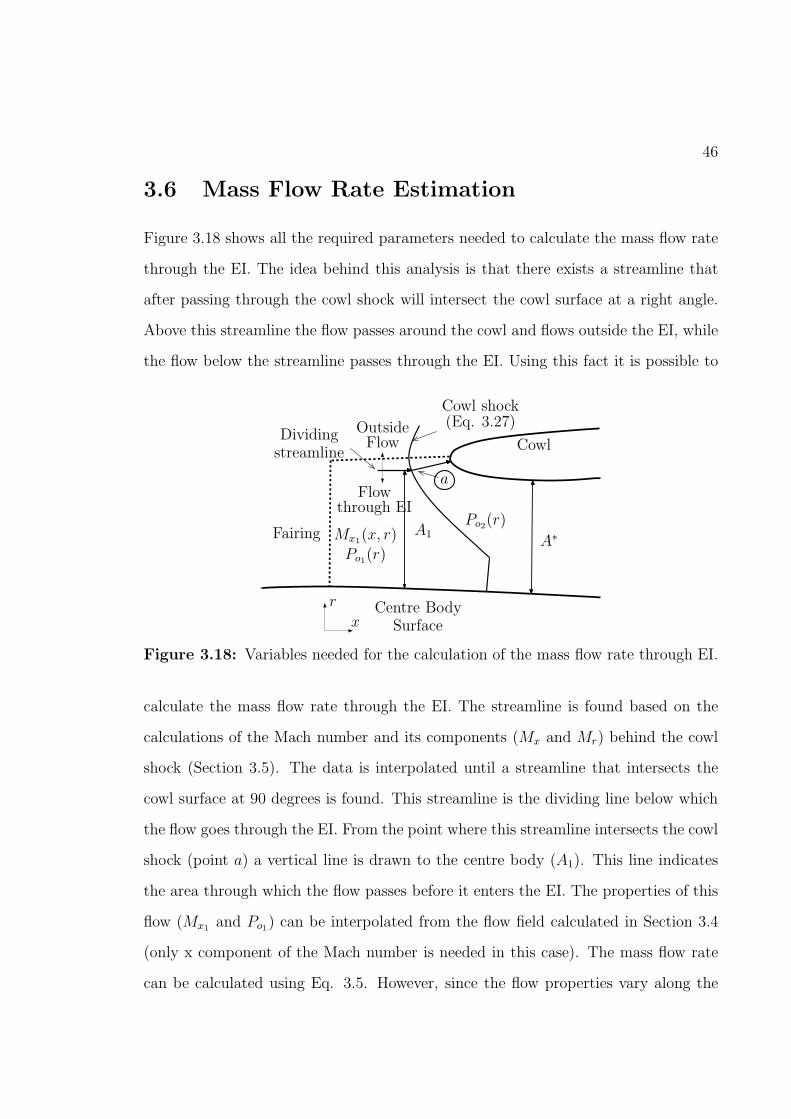
46
3.6 Mass Flow Rate Estimation
Figure 3.18 shows all the required parameters needed to calculate the mass flow rate
through the EI. The idea behind this analysis is that there exists a streamline that
after passing through the cowl shock will intersect the cowl surface at a right angle.
Above this streamline the flow passes around the cowl and flows outside the EI, while
the flow below the streamline passes through the EI. Using this fact it is possible to
Centre BodySurface
Fairing
Cowl
Cowl shock(Eq. 3.27)Outside
Flow
Flowthrough EI
A1A∗
Po2(r)Mx1(x, r)Po1(r)
a
Dividingstreamline
x
r
Figure 3.18: Variables needed for the calculation of the mass flow rate through EI.
calculate the mass flow rate through the EI. The streamline is found based on the
calculations of the Mach number and its components (Mx and Mr) behind the cowl
shock (Section 3.5). The data is interpolated until a streamline that intersects the
cowl surface at 90 degrees is found. This streamline is the dividing line below which
the flow goes through the EI. From the point where this streamline intersects the cowl
shock (point a) a vertical line is drawn to the centre body (A1). This line indicates
the area through which the flow passes before it enters the EI. The properties of this
flow (Mx1 and Po1) can be interpolated from the flow field calculated in Section 3.4
(only x component of the Mach number is needed in this case). The mass flow rate
can be calculated using Eq. 3.5. However, since the flow properties vary along the
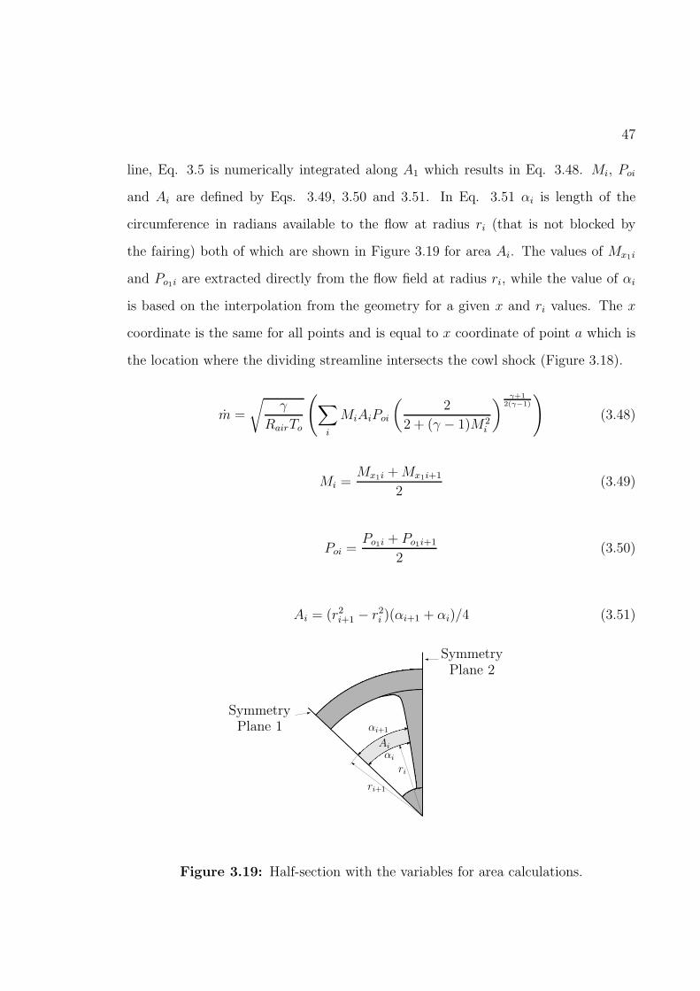
47
line, Eq. 3.5 is numerically integrated along A1 which results in Eq. 3.48. Mi, Poi
and Ai are defined by Eqs. 3.49, 3.50 and 3.51. In Eq. 3.51 αi is length of the
circumference in radians available to the flow at radius ri (that is not blocked by
the fairing) both of which are shown in Figure 3.19 for area Ai. The values of Mx1i
and Po1i are extracted directly from the flow field at radius ri, while the value of αi
is based on the interpolation from the geometry for a given x and ri values. The x
coordinate is the same for all points and is equal to x coordinate of point a which is
the location where the dividing streamline intersects the cowl shock (Figure 3.18).
m =
√
γ
RairTo
(
∑
i
MiAiPoi
(
2
2 + (γ − 1)M2i
)γ+1
2(γ−1)
)
(3.48)
Mi =Mx1i +Mx1i+1
2(3.49)
Poi =Po1i + Po1i+1
2(3.50)
Ai = (r2i+1 − r2i )(αi+1 + αi)/4 (3.51)
SymmetryPlane 2
SymmetryPlane 1
ri
ri+1
αi
αi+1
Ai
Figure 3.19: Half-section with the variables for area calculations.
48
To make sure that the calculated value of m does not exceed the choked mass
flow rate (m∗), the choked condition is calculated and the lesser of the two is used
for the final result. Eq. 3.52 is used to calculate m∗ where A∗ is the minimum cross
sectional area of the air passage through the EI taking into account the blockage by
the fairings, and Po2av is the averaged total pressure after the cowl shock which is
calculated in Section 3.5.
m∗ =
√
γ
RairTo
(
A∗Po2av
(
2
2 + (γ − 1)
)γ+1
2(γ−1)
)
(3.52)
For the cases where the cowl shock is not computed (e.g. the flow is subsonic after
the fairing shock) the m is calculated for the location at the entrance plane of the EI
(i.e. the point a is assumed to be located at the leading edge of the cowl). The Po2av
in Eq. 3.52 is also calculated at the entrance of the EI.
With this the calculations for the shock structure around the EI at the supersonic
flight conditions are complete. Along with the shock structure, the preceding analysis
allows to find an average Po entering the mixing duct, as well as an estimation of the
mass flow rate entering the engine to be calculated. The estimation method takes less
than 3 seconds to perform this analysis on a 3.0 GHz processor which is significantly
faster than a full 3D simulation.
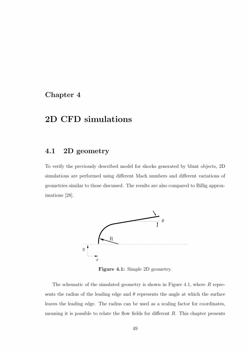
Chapter 4
2D CFD simulations
4.1 2D geometry
To verify the previously described model for shocks generated by blunt objects, 2D
simulations are performed using different Mach numbers and different variations of
geometries similar to those discussed. The results are also compared to Billig approx-
imations [28].
R
θ
x
y
Figure 4.1: Simple 2D geometry.
The schematic of the simulated geometry is shown in Figure 4.1, where R repre-
sents the radius of the leading edge and θ represents the angle at which the surface
leaves the leading edge. The radius can be used as a scaling factor for coordinates,
meaning it is possible to relate the flow fields for different R. This chapter presents
49
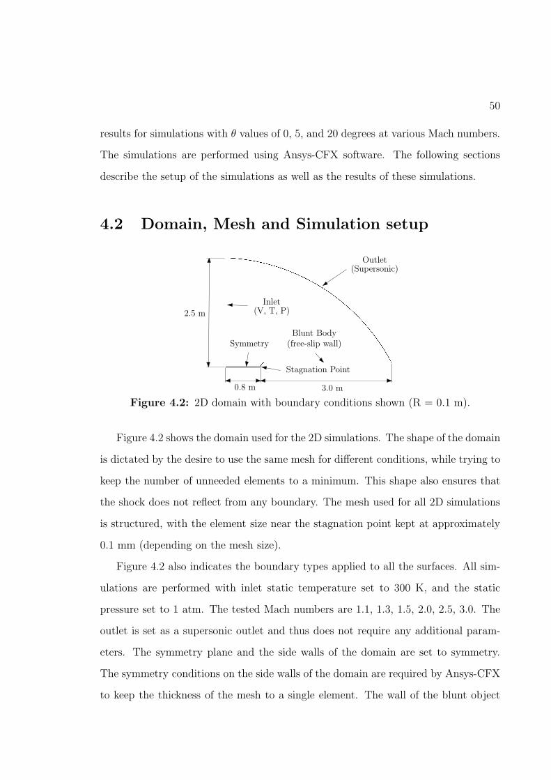
50
results for simulations with θ values of 0, 5, and 20 degrees at various Mach numbers.
The simulations are performed using Ansys-CFX software. The following sections
describe the setup of the simulations as well as the results of these simulations.
4.2 Domain, Mesh and Simulation setup
Outlet(Supersonic)
Inlet(V, T, P)
Blunt Body(free-slip wall)Symmetry
Stagnation Point
2.5 m
0.8 m 3.0 m
Figure 4.2: 2D domain with boundary conditions shown (R = 0.1 m).
Figure 4.2 shows the domain used for the 2D simulations. The shape of the domain
is dictated by the desire to use the same mesh for different conditions, while trying to
keep the number of unneeded elements to a minimum. This shape also ensures that
the shock does not reflect from any boundary. The mesh used for all 2D simulations
is structured, with the element size near the stagnation point kept at approximately
0.1 mm (depending on the mesh size).
Figure 4.2 also indicates the boundary types applied to all the surfaces. All sim-
ulations are performed with inlet static temperature set to 300 K, and the static
pressure set to 1 atm. The tested Mach numbers are 1.1, 1.3, 1.5, 2.0, 2.5, 3.0. The
outlet is set as a supersonic outlet and thus does not require any additional param-
eters. The symmetry plane and the side walls of the domain are set to symmetry.
The symmetry conditions on the side walls of the domain are required by Ansys-CFX
to keep the thickness of the mesh to a single element. The wall of the blunt object
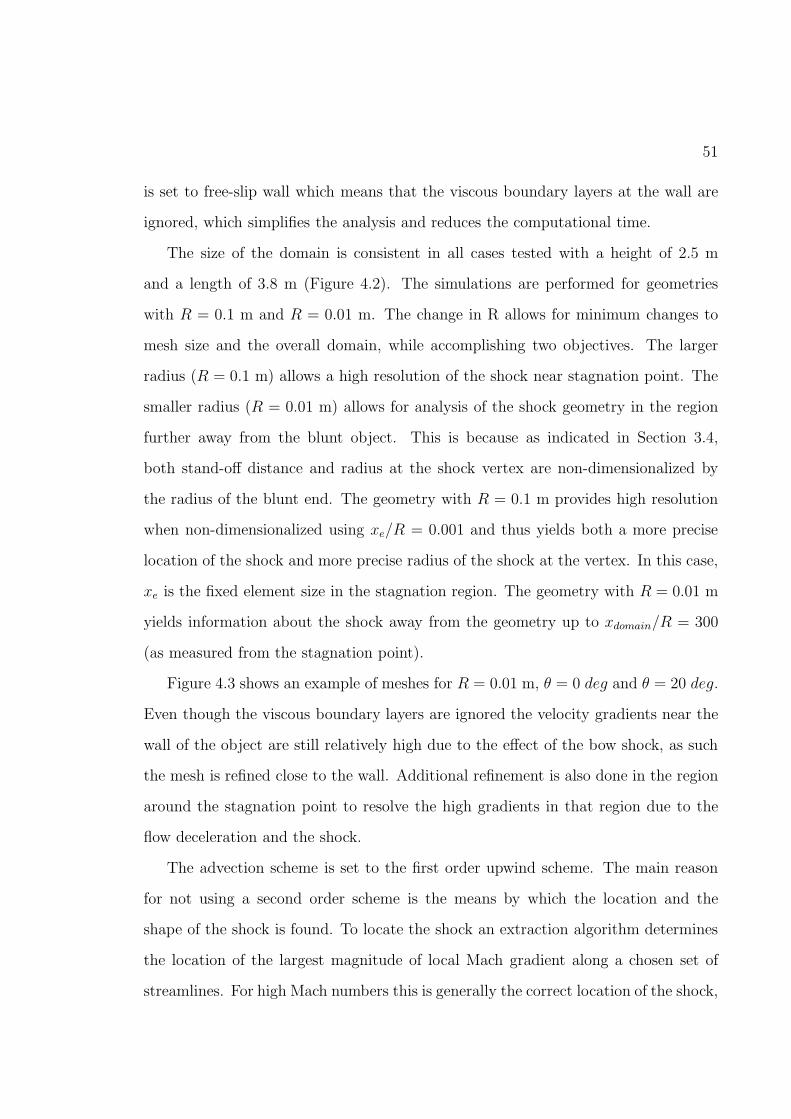
51
is set to free-slip wall which means that the viscous boundary layers at the wall are
ignored, which simplifies the analysis and reduces the computational time.
The size of the domain is consistent in all cases tested with a height of 2.5 m
and a length of 3.8 m (Figure 4.2). The simulations are performed for geometries
with R = 0.1 m and R = 0.01 m. The change in R allows for minimum changes to
mesh size and the overall domain, while accomplishing two objectives. The larger
radius (R = 0.1 m) allows a high resolution of the shock near stagnation point. The
smaller radius (R = 0.01 m) allows for analysis of the shock geometry in the region
further away from the blunt object. This is because as indicated in Section 3.4,
both stand-off distance and radius at the shock vertex are non-dimensionalized by
the radius of the blunt end. The geometry with R = 0.1 m provides high resolution
when non-dimensionalized using xe/R = 0.001 and thus yields both a more precise
location of the shock and more precise radius of the shock at the vertex. In this case,
xe is the fixed element size in the stagnation region. The geometry with R = 0.01 m
yields information about the shock away from the geometry up to xdomain/R = 300
(as measured from the stagnation point).
Figure 4.3 shows an example of meshes for R = 0.01 m, θ = 0 deg and θ = 20 deg.
Even though the viscous boundary layers are ignored the velocity gradients near the
wall of the object are still relatively high due to the effect of the bow shock, as such
the mesh is refined close to the wall. Additional refinement is also done in the region
around the stagnation point to resolve the high gradients in that region due to the
flow deceleration and the shock.
The advection scheme is set to the first order upwind scheme. The main reason
for not using a second order scheme is the means by which the location and the
shape of the shock is found. To locate the shock an extraction algorithm determines
the location of the largest magnitude of local Mach gradient along a chosen set of
streamlines. For high Mach numbers this is generally the correct location of the shock,
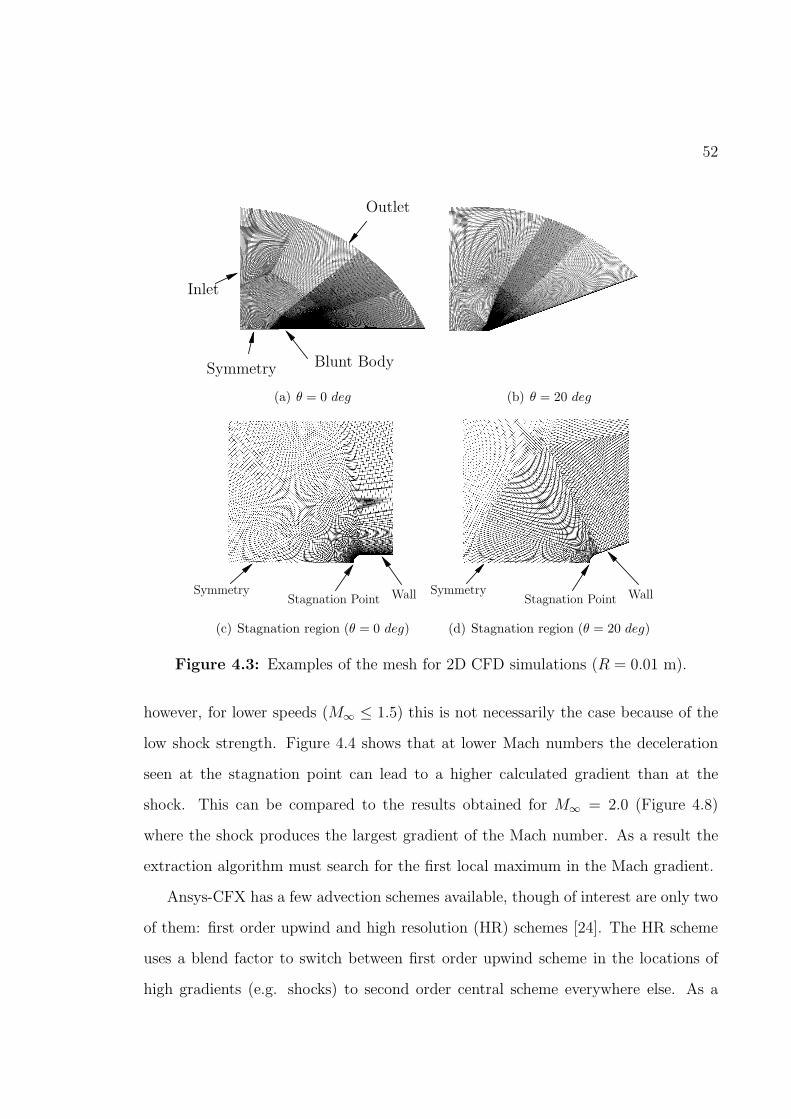
52
Symmetry
Inlet
Blunt Body
Outlet
(a) θ = 0 deg (b) θ = 20 deg
SymmetryStagnation Point Wall
(c) Stagnation region (θ = 0 deg)
SymmetryStagnation Point Wall
(d) Stagnation region (θ = 20 deg)
Figure 4.3: Examples of the mesh for 2D CFD simulations (R = 0.01 m).
however, for lower speeds (M∞ ≤ 1.5) this is not necessarily the case because of the
low shock strength. Figure 4.4 shows that at lower Mach numbers the deceleration
seen at the stagnation point can lead to a higher calculated gradient than at the
shock. This can be compared to the results obtained for M∞ = 2.0 (Figure 4.8)
where the shock produces the largest gradient of the Mach number. As a result the
extraction algorithm must search for the first local maximum in the Mach gradient.
Ansys-CFX has a few advection schemes available, though of interest are only two
of them: first order upwind and high resolution (HR) schemes [24]. The HR scheme
uses a blend factor to switch between first order upwind scheme in the locations of
high gradients (e.g. shocks) to second order central scheme everywhere else. As a
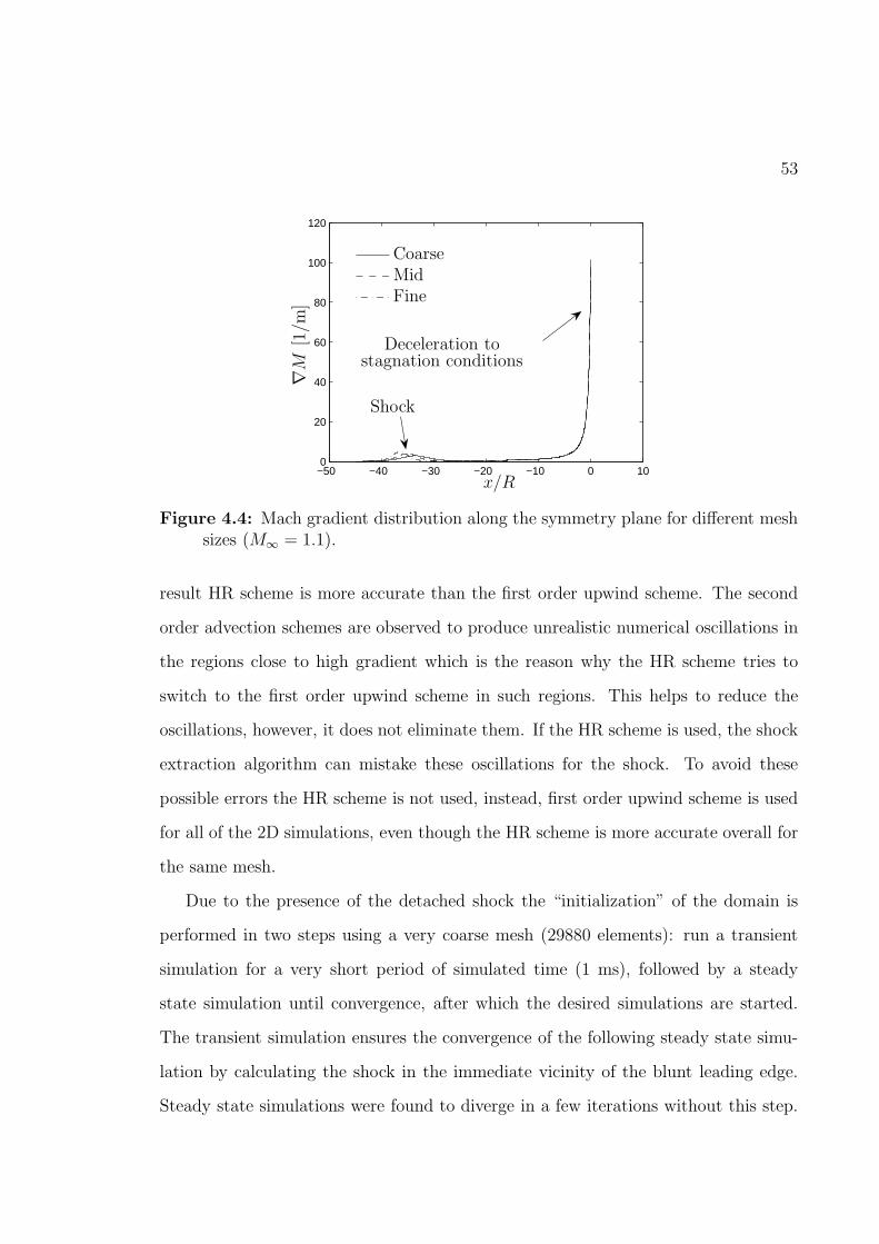
53
−50 −40 −30 −20 −10 0 100
20
40
60
80
100
120
∇M
[1/m
]
x/R
CoarseMidFine
Shock
Deceleration tostagnation conditions
Figure 4.4: Mach gradient distribution along the symmetry plane for different meshsizes (M∞ = 1.1).
result HR scheme is more accurate than the first order upwind scheme. The second
order advection schemes are observed to produce unrealistic numerical oscillations in
the regions close to high gradient which is the reason why the HR scheme tries to
switch to the first order upwind scheme in such regions. This helps to reduce the
oscillations, however, it does not eliminate them. If the HR scheme is used, the shock
extraction algorithm can mistake these oscillations for the shock. To avoid these
possible errors the HR scheme is not used, instead, first order upwind scheme is used
for all of the 2D simulations, even though the HR scheme is more accurate overall for
the same mesh.
Due to the presence of the detached shock the “initialization” of the domain is
performed in two steps using a very coarse mesh (29880 elements): run a transient
simulation for a very short period of simulated time (1 ms), followed by a steady
state simulation until convergence, after which the desired simulations are started.
The transient simulation ensures the convergence of the following steady state simu-
lation by calculating the shock in the immediate vicinity of the blunt leading edge.
Steady state simulations were found to diverge in a few iterations without this step.
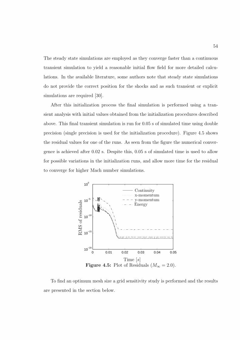
54
The steady state simulations are employed as they converge faster than a continuous
transient simulation to yield a reasonable initial flow field for more detailed calcu-
lations. In the available literature, some authors note that steady state simulations
do not provide the correct position for the shocks and as such transient or explicit
simulations are required [30].
After this initialization process the final simulation is performed using a tran-
sient analysis with initial values obtained from the initialization procedures described
above. This final transient simulation is run for 0.05 s of simulated time using double
precision (single precision is used for the initialization procedure). Figure 4.5 shows
the residual values for one of the runs. As seen from the figure the numerical conver-
gence is achieved after 0.02 s. Despite this, 0.05 s of simulated time is used to allow
for possible variations in the initialization runs, and allow more time for the residual
to converge for higher Mach number simulations.
0 0.01 0.02 0.03 0.04 0.0510
−20
10−15
10−10
10−5
100
Time [s]
RMSof
residuals
Continuityx-momentumy-momentumEnergy
Figure 4.5: Plot of Residuals (M∞ = 2.0).
To find an optimum mesh size a grid sensitivity study is performed and the results
are presented in the section below.
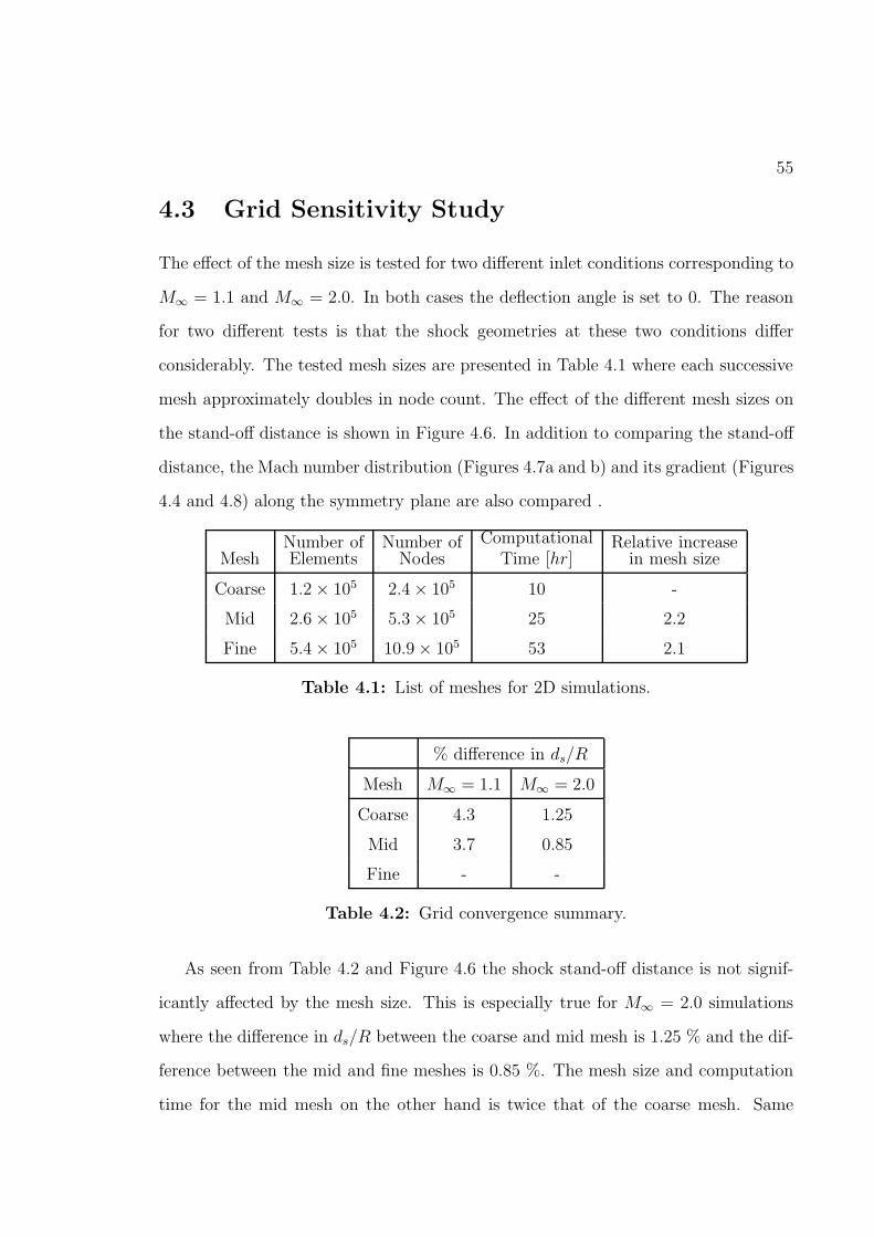
55
4.3 Grid Sensitivity Study
The effect of the mesh size is tested for two different inlet conditions corresponding to
M∞ = 1.1 and M∞ = 2.0. In both cases the deflection angle is set to 0. The reason
for two different tests is that the shock geometries at these two conditions differ
considerably. The tested mesh sizes are presented in Table 4.1 where each successive
mesh approximately doubles in node count. The effect of the different mesh sizes on
the stand-off distance is shown in Figure 4.6. In addition to comparing the stand-off
distance, the Mach number distribution (Figures 4.7a and b) and its gradient (Figures
4.4 and 4.8) along the symmetry plane are also compared .
MeshNumber ofElements
Number ofNodes
ComputationalTime [hr]
Relative increasein mesh size
Coarse 1.2× 10⁵ 2.4× 10⁵ 10 -
Mid 2.6× 10⁵ 5.3× 10⁵ 25 2.2
Fine 5.4× 10⁵ 10.9× 10⁵ 53 2.1
Table 4.1: List of meshes for 2D simulations.
% difference in ds/R
Mesh M∞ = 1.1 M∞ = 2.0
Coarse 4.3 1.25
Mid 3.7 0.85
Fine - -
Table 4.2: Grid convergence summary.
As seen from Table 4.2 and Figure 4.6 the shock stand-off distance is not signif-
icantly affected by the mesh size. This is especially true for M∞ = 2.0 simulations
where the difference in ds/R between the coarse and mid mesh is 1.25 % and the dif-
ference between the mid and fine meshes is 0.85 %. The mesh size and computation
time for the mid mesh on the other hand is twice that of the coarse mesh. Same
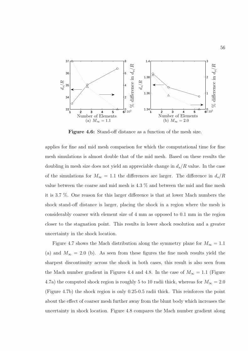
56
1 2 3 4 5 633
34
35
36
37
1 2 3 4 5 60
2
4
6
8
Number of Elements
ds/R
%difference
inds/R
×105
(a) M∞ = 1.1
1 2 3 4 5 61.34
1.36
1.38
1.4
1 2 3 4 5 60
1
2
3
Number of Elements
ds/R
%difference
inds/R
×105
(b) M∞ = 2.0
Figure 4.6: Stand-off distance as a function of the mesh size.
applies for fine and mid mesh comparison for which the computational time for fine
mesh simulations is almost double that of the mid mesh. Based on these results the
doubling in mesh size does not yield an appreciable change in ds/R value. In the case
of the simulations for M∞ = 1.1 the differences are larger. The difference in ds/R
value between the coarse and mid mesh is 4.3 % and between the mid and fine mesh
it is 3.7 %. One reason for this larger difference is that at lower Mach numbers the
shock stand-off distance is larger, placing the shock in a region where the mesh is
considerably coarser with element size of 4 mm as opposed to 0.1 mm in the region
closer to the stagnation point. This results in lower shock resolution and a greater
uncertainty in the shock location.
Figure 4.7 shows the Mach distribution along the symmetry plane for M∞ = 1.1
(a) and M∞ = 2.0 (b). As seen from these figures the fine mesh results yield the
sharpest discontinuity across the shock in both cases, this result is also seen from
the Mach number gradient in Figures 4.4 and 4.8. In the case of M∞ = 1.1 (Figure
4.7a) the computed shock region is roughly 5 to 10 radii thick, whereas forM∞ = 2.0
(Figure 4.7b) the shock region is only 0.25-0.5 radii thick. This reinforces the point
about the effect of coarser mesh further away from the blunt body which increases the
uncertainty in shock location. Figure 4.8 compares the Mach number gradient along
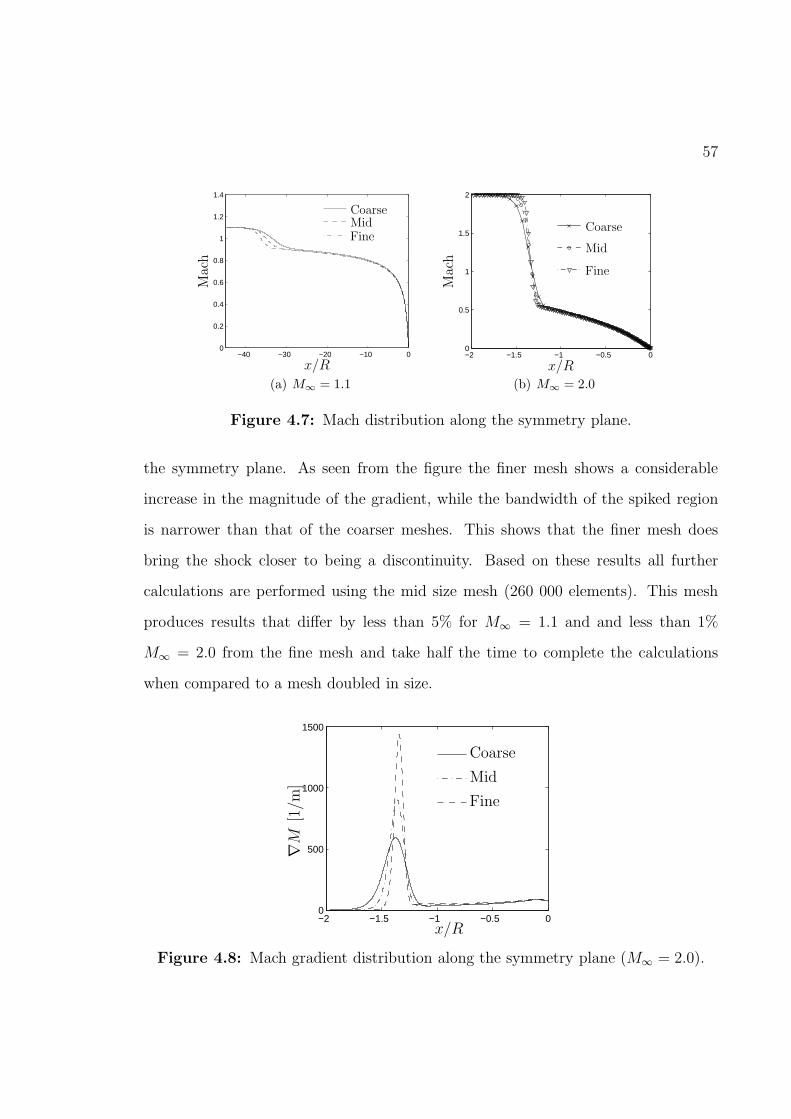
57
−40 −30 −20 −10 00
0.2
0.4
0.6
0.8
1
1.2
1.4
Mach
x/R
CoarseMidFine
(a) M∞ = 1.1
−2 −1.5 −1 −0.5 00
0.5
1
1.5
2
Mach
x/R
Coarse
Mid
Fine
(b) M∞ = 2.0
Figure 4.7: Mach distribution along the symmetry plane.
the symmetry plane. As seen from the figure the finer mesh shows a considerable
increase in the magnitude of the gradient, while the bandwidth of the spiked region
is narrower than that of the coarser meshes. This shows that the finer mesh does
bring the shock closer to being a discontinuity. Based on these results all further
calculations are performed using the mid size mesh (260 000 elements). This mesh
produces results that differ by less than 5% for M∞ = 1.1 and and less than 1%
M∞ = 2.0 from the fine mesh and take half the time to complete the calculations
when compared to a mesh doubled in size.
−2 −1.5 −1 −0.5 00
500
1000
1500
∇M
[1/m
]
x/R
Coarse
Mid
Fine
Figure 4.8: Mach gradient distribution along the symmetry plane (M∞ = 2.0).
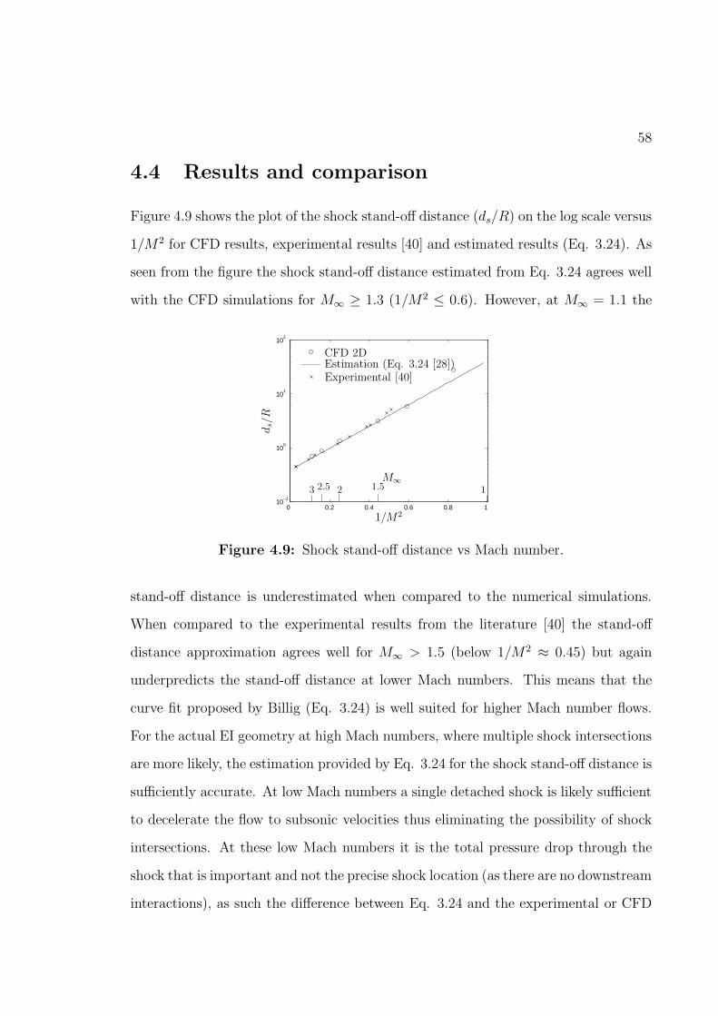
58
4.4 Results and comparison
Figure 4.9 shows the plot of the shock stand-off distance (ds/R) on the log scale versus
1/M2 for CFD results, experimental results [40] and estimated results (Eq. 3.24). As
seen from the figure the shock stand-off distance estimated from Eq. 3.24 agrees well
with the CFD simulations for M∞ ≥ 1.3 (1/M2 ≤ 0.6). However, at M∞ = 1.1 the
0 0.2 0.4 0.6 0.8 1 10
−1
100
101
102
1/M2
ds/R
CFD 2DEstimation (Eq. 3.24 [28])Experimental [40]
M∞
3 2.5 2 1.5 1
Figure 4.9: Shock stand-off distance vs Mach number.
stand-off distance is underestimated when compared to the numerical simulations.
When compared to the experimental results from the literature [40] the stand-off
distance approximation agrees well for M∞ > 1.5 (below 1/M2 ≈ 0.45) but again
underpredicts the stand-off distance at lower Mach numbers. This means that the
curve fit proposed by Billig (Eq. 3.24) is well suited for higher Mach number flows.
For the actual EI geometry at high Mach numbers, where multiple shock intersections
are more likely, the estimation provided by Eq. 3.24 for the shock stand-off distance is
sufficiently accurate. At low Mach numbers a single detached shock is likely sufficient
to decelerate the flow to subsonic velocities thus eliminating the possibility of shock
intersections. At these low Mach numbers it is the total pressure drop through the
shock that is important and not the precise shock location (as there are no downstream
interactions), as such the difference between Eq. 3.24 and the experimental or CFD
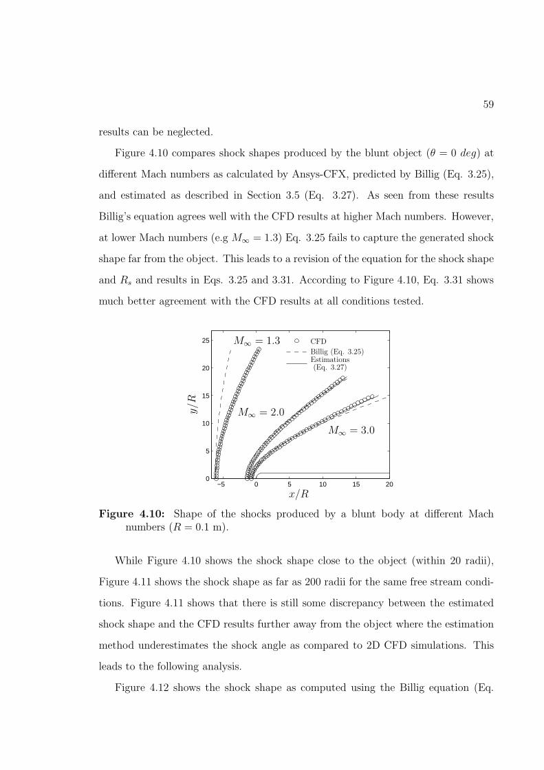
59
results can be neglected.
Figure 4.10 compares shock shapes produced by the blunt object (θ = 0 deg) at
different Mach numbers as calculated by Ansys-CFX, predicted by Billig (Eq. 3.25),
and estimated as described in Section 3.5 (Eq. 3.27). As seen from these results
Billig’s equation agrees well with the CFD results at higher Mach numbers. However,
at lower Mach numbers (e.g M∞ = 1.3) Eq. 3.25 fails to capture the generated shock
shape far from the object. This leads to a revision of the equation for the shock shape
and Rs and results in Eqs. 3.25 and 3.31. According to Figure 4.10, Eq. 3.31 shows
much better agreement with the CFD results at all conditions tested.
−5 0 5 10 15 200
5
10
15
20
25
x/R
y/R
CFD
Billig (Eq. 3.25)Estimations(Eq. 3.27)
M∞ = 1.3
M∞ = 2.0
M∞ = 3.0
Figure 4.10: Shape of the shocks produced by a blunt body at different Machnumbers (R = 0.1 m).
While Figure 4.10 shows the shock shape close to the object (within 20 radii),
Figure 4.11 shows the shock shape as far as 200 radii for the same free stream condi-
tions. Figure 4.11 shows that there is still some discrepancy between the estimated
shock shape and the CFD results further away from the object where the estimation
method underestimates the shock angle as compared to 2D CFD simulations. This
leads to the following analysis.
Figure 4.12 shows the shock shape as computed using the Billig equation (Eq.
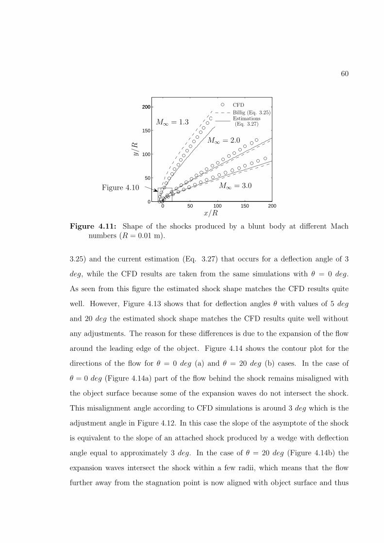
60
0 50 100 150 2000
50
100
150
200200
x/R
y/R
CFD
Billig (Eq. 3.25)Estimations(Eq. 3.27)M∞ = 1.3
M∞ = 2.0
M∞ = 3.0Figure 4.10
Figure 4.11: Shape of the shocks produced by a blunt body at different Machnumbers (R = 0.01 m).
3.25) and the current estimation (Eq. 3.27) that occurs for a deflection angle of 3
deg, while the CFD results are taken from the same simulations with θ = 0 deg.
As seen from this figure the estimated shock shape matches the CFD results quite
well. However, Figure 4.13 shows that for deflection angles θ with values of 5 deg
and 20 deg the estimated shock shape matches the CFD results quite well without
any adjustments. The reason for these differences is due to the expansion of the flow
around the leading edge of the object. Figure 4.14 shows the contour plot for the
directions of the flow for θ = 0 deg (a) and θ = 20 deg (b) cases. In the case of
θ = 0 deg (Figure 4.14a) part of the flow behind the shock remains misaligned with
the object surface because some of the expansion waves do not intersect the shock.
This misalignment angle according to CFD simulations is around 3 deg which is the
adjustment angle in Figure 4.12. In this case the slope of the asymptote of the shock
is equivalent to the slope of an attached shock produced by a wedge with deflection
angle equal to approximately 3 deg. In the case of θ = 20 deg (Figure 4.14b) the
expansion waves intersect the shock within a few radii, which means that the flow
further away from the stagnation point is now aligned with object surface and thus
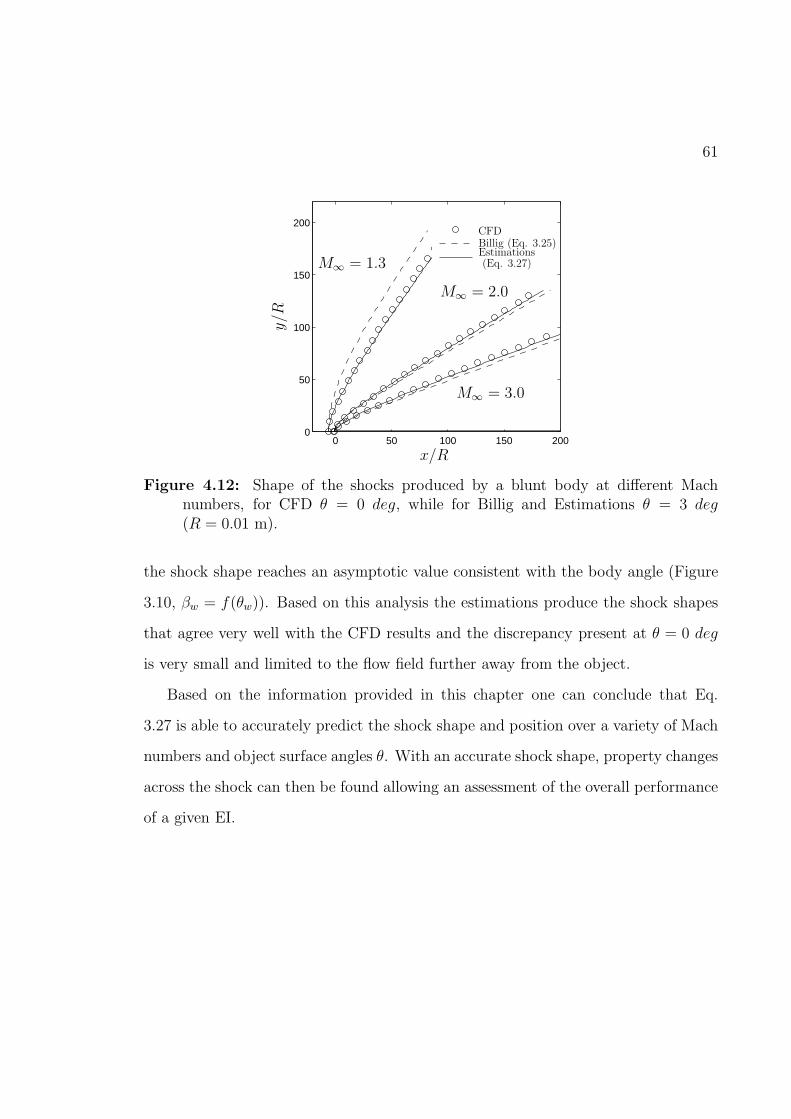
61
0 50 100 150 2000
50
100
150
200
x/R
y/R
CFDBillig (Eq. 3.25)Estimations(Eq. 3.27)M∞ = 1.3
M∞ = 2.0
M∞ = 3.0
Figure 4.12: Shape of the shocks produced by a blunt body at different Machnumbers, for CFD θ = 0 deg, while for Billig and Estimations θ = 3 deg(R = 0.01 m).
the shock shape reaches an asymptotic value consistent with the body angle (Figure
3.10, βw = f(θw)). Based on this analysis the estimations produce the shock shapes
that agree very well with the CFD results and the discrepancy present at θ = 0 deg
is very small and limited to the flow field further away from the object.
Based on the information provided in this chapter one can conclude that Eq.
3.27 is able to accurately predict the shock shape and position over a variety of Mach
numbers and object surface angles θ. With an accurate shock shape, property changes
across the shock can then be found allowing an assessment of the overall performance
of a given EI.
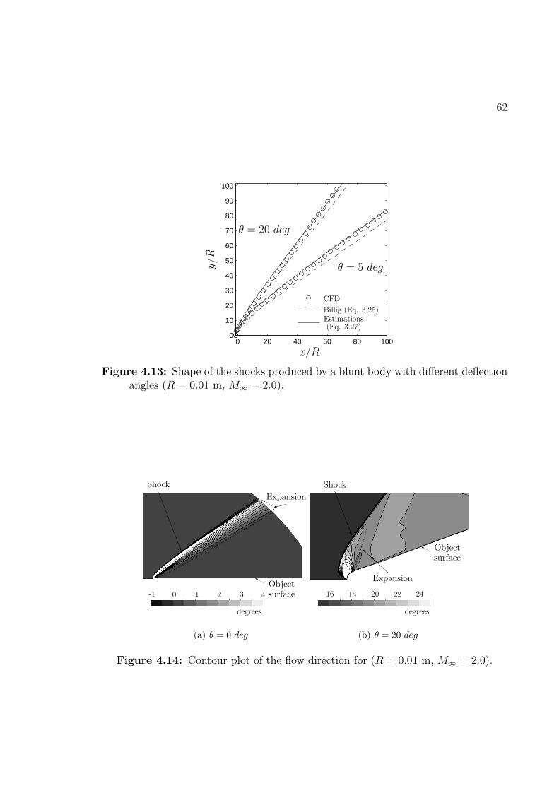
62
0 20 40 60 80 1000
10
20
30
40
50
60
70
80
90
100
x/R
y/R
CFD
Billig (Eq. 3.25)Estimations(Eq. 3.27)
θ = 5 deg
θ = 20 deg
Figure 4.13: Shape of the shocks produced by a blunt body with different deflectionangles (R = 0.01 m, M∞ = 2.0).
degrees
-1 0 1 2 3 4
Expansion
Shock
Objectsurface
(a) θ = 0 deg
degrees
16 18 20 22 24
Expansion
Shock
Objectsurface
(b) θ = 20 deg
Figure 4.14: Contour plot of the flow direction for (R = 0.01 m, M∞ = 2.0).
Chapter 5
3D CFD simulations
5.1 Overview
This chapter describes the 3D simulations of the EI and also compares the results from
these simulations to the ones obtained from the estimation method. The comparison
is performed for the shock shapes, total pressure drop and the mass flow rate through
the EI.
5.2 3D Simulation Setup
The modelling of the geometry is performed using ICEM CFD software [23]. Due
to the symmetry of the RBCC EI only one eighth is modelled. This allows for a
finer mesh to be used without excessively raising the computation times. Figure
5.1 shows the section that is being modelled with symmetry planes indicated, while
Figure 5.2 shows the computational domain with the boundary conditions. Due to
issues with the structured mesh at the nose tip of the centre body the geometry
is slightly modified as shown in Figure 5.3. The structured mesh for this analysis
is constructed using hexahedron elements. The sharp nose tip of the centre body
requires the use of “collapsed” elements, that is one of the faces of these hexahedron
63
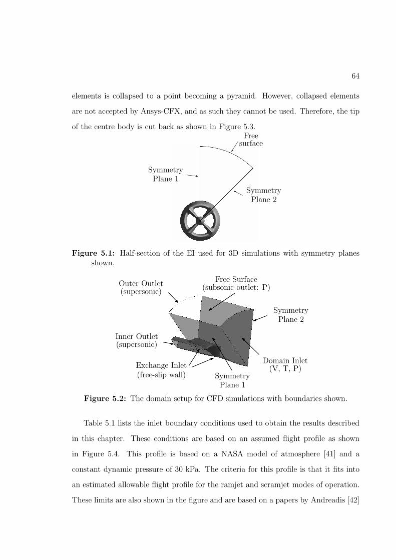
64
elements is collapsed to a point becoming a pyramid. However, collapsed elements
are not accepted by Ansys-CFX, and as such they cannot be used. Therefore, the tip
of the centre body is cut back as shown in Figure 5.3.
SymmetryPlane 2
SymmetryPlane 1
Freesurface
Figure 5.1: Half-section of the EI used for 3D simulations with symmetry planesshown.
Exchange Inlet(free-slip wall)
Domain Inlet(V, T, P)
SymmetryPlane 1
SymmetryPlane 2
Outer Outlet(supersonic)
Inner Outlet(supersonic)
Free Surface(subsonic outlet: P)
Figure 5.2: The domain setup for CFD simulations with boundaries shown.
Table 5.1 lists the inlet boundary conditions used to obtain the results described
in this chapter. These conditions are based on an assumed flight profile as shown
in Figure 5.4. This profile is based on a NASA model of atmosphere [41] and a
constant dynamic pressure of 30 kPa. The criteria for this profile is that it fits into
an estimated allowable flight profile for the ramjet and scramjet modes of operation.
These limits are also shown in the figure and are based on a papers by Andreadis [42]
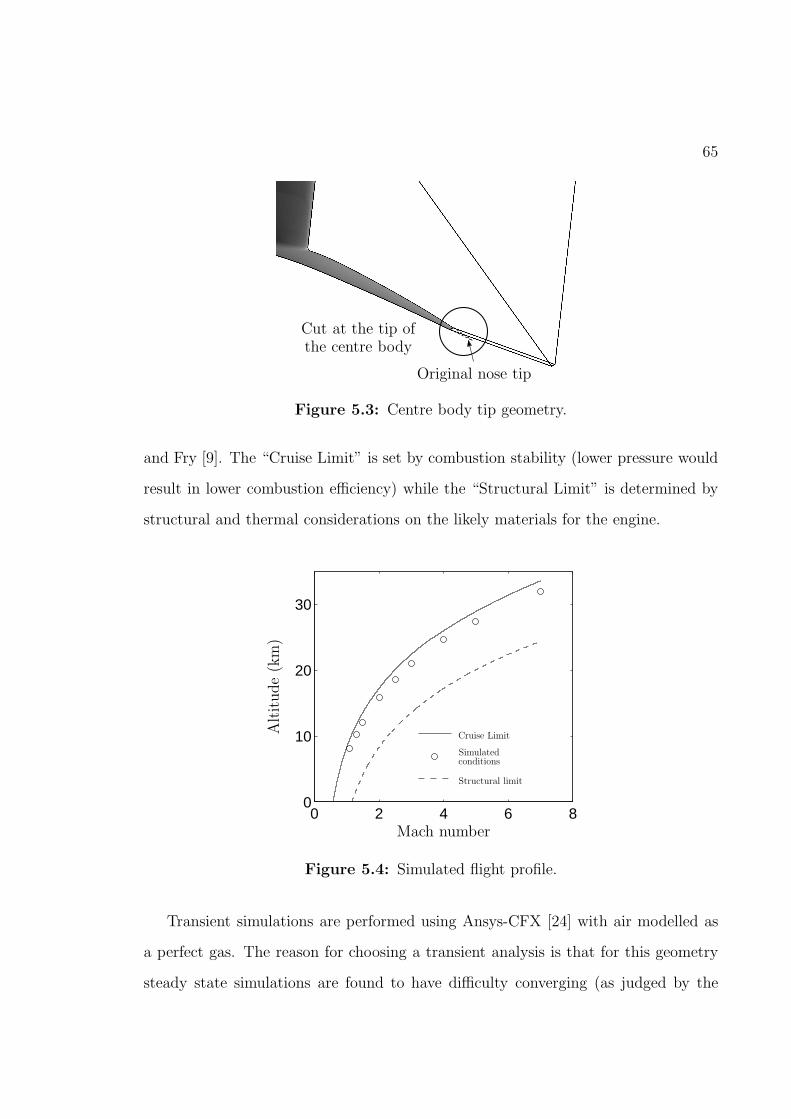
65
Cut at the tip ofthe centre body
Original nose tip
Figure 5.3: Centre body tip geometry.
and Fry [9]. The “Cruise Limit” is set by combustion stability (lower pressure would
result in lower combustion efficiency) while the “Structural Limit” is determined by
structural and thermal considerations on the likely materials for the engine.
0 2 4 6 80
10
20
30
Altitude(km)
Mach number
Cruise Limit
Simulatedconditions
Structural limit
Figure 5.4: Simulated flight profile.
Transient simulations are performed using Ansys-CFX [24] with air modelled as
a perfect gas. The reason for choosing a transient analysis is that for this geometry
steady state simulations are found to have difficulty converging (as judged by the
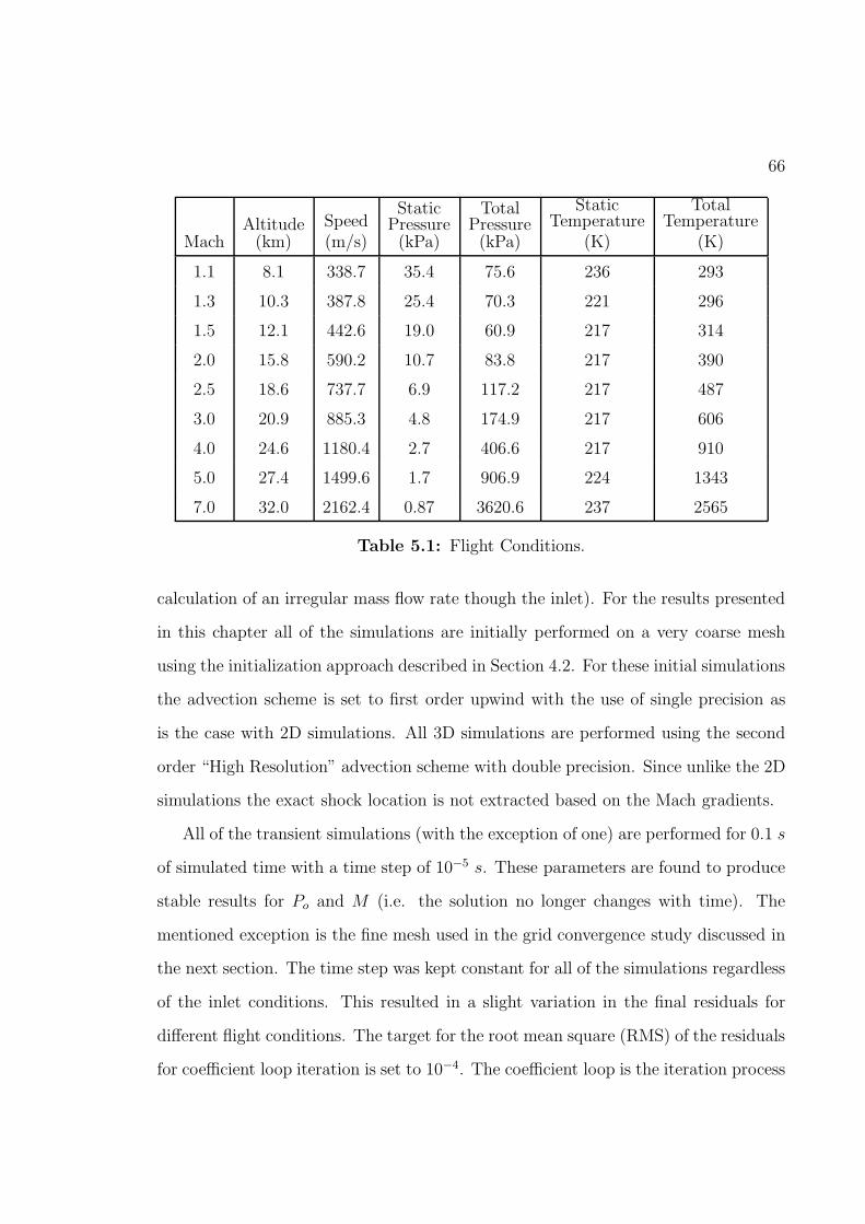
66
MachAltitude(km)
Speed(m/s)
StaticPressure(kPa)
TotalPressure(kPa)
StaticTemperature
(K)
TotalTemperature
(K)
1.1 8.1 338.7 35.4 75.6 236 293
1.3 10.3 387.8 25.4 70.3 221 296
1.5 12.1 442.6 19.0 60.9 217 314
2.0 15.8 590.2 10.7 83.8 217 390
2.5 18.6 737.7 6.9 117.2 217 487
3.0 20.9 885.3 4.8 174.9 217 606
4.0 24.6 1180.4 2.7 406.6 217 910
5.0 27.4 1499.6 1.7 906.9 224 1343
7.0 32.0 2162.4 0.87 3620.6 237 2565
Table 5.1: Flight Conditions.
calculation of an irregular mass flow rate though the inlet). For the results presented
in this chapter all of the simulations are initially performed on a very coarse mesh
using the initialization approach described in Section 4.2. For these initial simulations
the advection scheme is set to first order upwind with the use of single precision as
is the case with 2D simulations. All 3D simulations are performed using the second
order “High Resolution” advection scheme with double precision. Since unlike the 2D
simulations the exact shock location is not extracted based on the Mach gradients.
All of the transient simulations (with the exception of one) are performed for 0.1 s
of simulated time with a time step of 10−5 s. These parameters are found to produce
stable results for Po and M (i.e. the solution no longer changes with time). The
mentioned exception is the fine mesh used in the grid convergence study discussed in
the next section. The time step was kept constant for all of the simulations regardless
of the inlet conditions. This resulted in a slight variation in the final residuals for
different flight conditions. The target for the root mean square (RMS) of the residuals
for coefficient loop iteration is set to 10−4. The coefficient loop is the iteration process
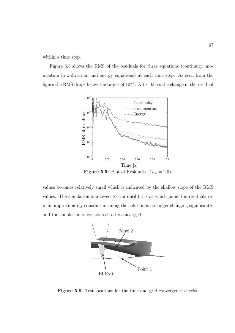
67
within a time step.
Figure 5.5 shows the RMS of the residuals for three equations (continuity, mo-
mentum in x-direction and energy equations) at each time step. As seen from the
figure the RMS drops below the target of 10−4. After 0.05 s the change in the residual
0 0.02 0.04 0.06 0.08 0.110
−8
10−7
10−6
10−5
10−4
Time [s]
RMSof
residuals
Continuity
x-momentum
Energy
Figure 5.5: Plot of Residuals (M∞ = 2.0).
values becomes relatively small which is indicated by the shallow slope of the RMS
values. The simulation is allowed to run until 0.1 s at which point the residuals re-
main approximately constant meaning the solution is no longer changing significantly
and the simulation is considered to be converged.
Point 2
Point 1EI Exit
Figure 5.6: Test locations for the time and grid convergence checks.
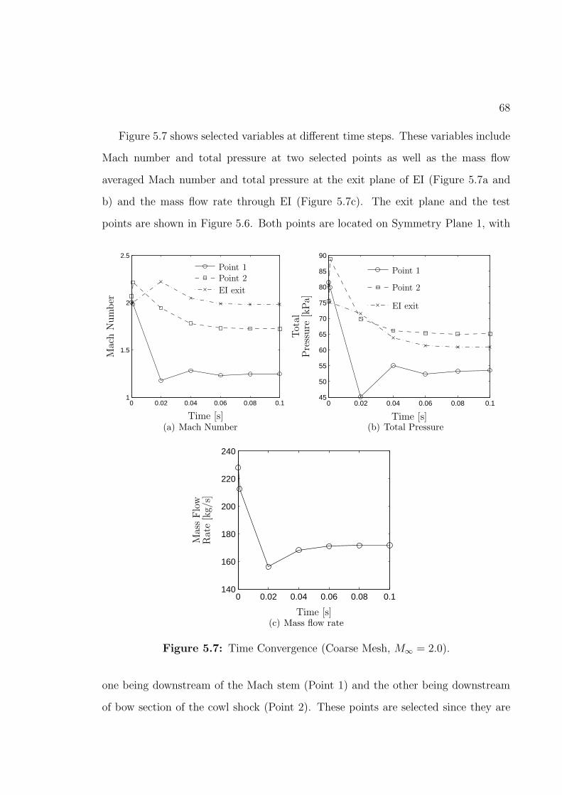
68
Figure 5.7 shows selected variables at different time steps. These variables include
Mach number and total pressure at two selected points as well as the mass flow
averaged Mach number and total pressure at the exit plane of EI (Figure 5.7a and
b) and the mass flow rate through EI (Figure 5.7c). The exit plane and the test
points are shown in Figure 5.6. Both points are located on Symmetry Plane 1, with
0 0.02 0.04 0.06 0.08 0.11
1.5
2
2.5
Time [s]
MachNumber
Point 1Point 2
EI exit
(a) Mach Number
0 0.02 0.04 0.06 0.08 0.145
50
55
60
65
70
75
80
85
90
Time [s]
Total
Pressure
[kPa]
Point 1
Point 2
EI exit
(b) Total Pressure
0 0.02 0.04 0.06 0.08 0.1140
160
180
200
220
240
Time [s]
MassFlow
Rate[kg/s]
(c) Mass flow rate
Figure 5.7: Time Convergence (Coarse Mesh, M∞ = 2.0).
one being downstream of the Mach stem (Point 1) and the other being downstream
of bow section of the cowl shock (Point 2). These points are selected since they are
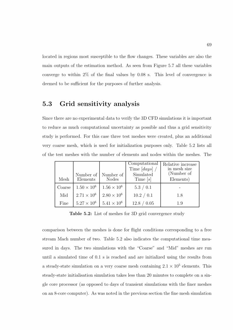
69
located in regions most susceptible to the flow changes. These variables are also the
main outputs of the estimation method. As seen from Figure 5.7 all these variables
converge to within 2% of the final values by 0.08 s. This level of convergence is
deemed to be sufficient for the purposes of further analysis.
5.3 Grid sensitivity analysis
Since there are no experimental data to verify the 3D CFD simulations it is important
to reduce as much computational uncertainty as possible and thus a grid sensitivity
study is performed. For this case three test meshes were created, plus an additional
very coarse mesh, which is used for initialization purposes only. Table 5.2 lists all
of the test meshes with the number of elements and nodes within the meshes. The
MeshNumber ofElements
Number ofNodes
ComputationalTime [days] /SimulatedTime [s]
Relative increasein mesh size(Number of
Elements)
Coarse 1.50× 10⁶ 1.56× 10⁶ 5.3 / 0.1 -
Mid 2.71× 10⁶ 2.80× 10⁶ 10.2 / 0.1 1.8
Fine 5.27× 10⁶ 5.41× 10⁶ 12.8 / 0.05 1.9
Table 5.2: List of meshes for 3D grid convergence study
comparison between the meshes is done for flight conditions corresponding to a free
stream Mach number of two. Table 5.2 also indicates the computational time mea-
sured in days. The two simulations with the “Coarse” and “Mid” meshes are run
until a simulated time of 0.1 s is reached and are initialized using the results from
a steady-state simulation on a very coarse mesh containing 2.1× 10⁵ elements. This
steady-state initialisation simulation takes less than 20 minutes to complete on a sin-
gle core processor (as opposed to days of transient simulations with the finer meshes
on an 8-core computer). As was noted in the previous section the fine mesh simulation
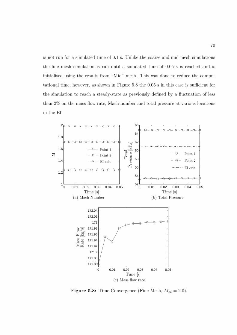
70
is not run for a simulated time of 0.1 s. Unlike the coarse and mid mesh simulations
the fine mesh simulation is run until a simulated time of 0.05 s is reached and is
initialised using the results from “Mid” mesh. This was done to reduce the compu-
tational time, however, as shown in Figure 5.8 the 0.05 s in this case is sufficient for
the simulation to reach a steady-state as previously defined by a fluctuation of less
than 2% on the mass flow rate, Mach number and total pressure at various locations
in the EI.
0 0.01 0.02 0.03 0.04 0.051
1.2
1.4
1.6
1.8
2
Time [s]
M
Point 1
Point 2
EI exit
(a) Mach Number
0 0.01 0.02 0.03 0.04 0.0552
54
56
58
60
62
64
66
Time [s]
Total
Pressure
[kPa]
Point 1
Point 2
EI exit
(b) Total Pressure
0 0.01 0.02 0.03 0.04 0.05
171.86
171.88
171.9
171.92
171.94
171.96
171.98
172
172.02
172.04
Time [s]
MassFlow
Rate[kg/s]
(c) Mass flow rate
Figure 5.8: Time Convergence (Fine Mesh, M∞ = 2.0).
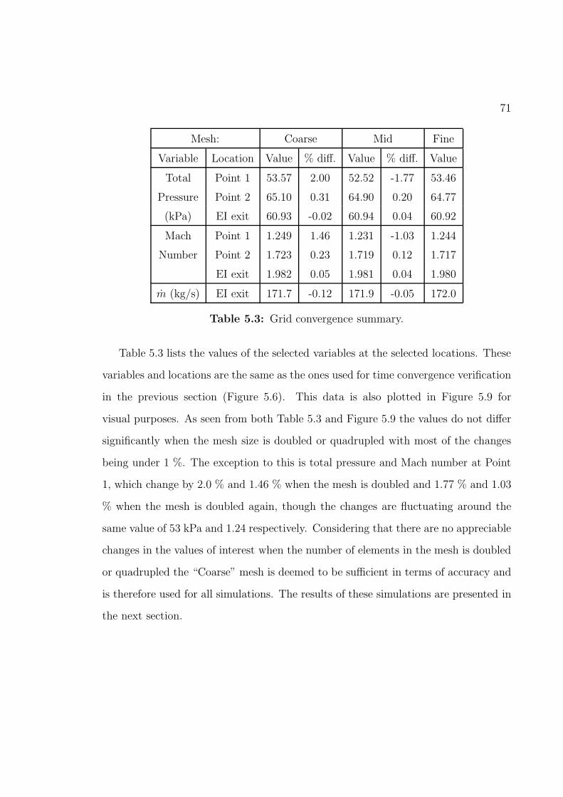
71
Mesh: Coarse Mid Fine
Variable Location Value % diff. Value % diff. Value
Total Point 1 53.57 2.00 52.52 -1.77 53.46
Pressure Point 2 65.10 0.31 64.90 0.20 64.77
(kPa) EI exit 60.93 -0.02 60.94 0.04 60.92
Mach Point 1 1.249 1.46 1.231 -1.03 1.244
Number Point 2 1.723 0.23 1.719 0.12 1.717
EI exit 1.982 0.05 1.981 0.04 1.980
m (kg/s) EI exit 171.7 -0.12 171.9 -0.05 172.0
Table 5.3: Grid convergence summary.
Table 5.3 lists the values of the selected variables at the selected locations. These
variables and locations are the same as the ones used for time convergence verification
in the previous section (Figure 5.6). This data is also plotted in Figure 5.9 for
visual purposes. As seen from both Table 5.3 and Figure 5.9 the values do not differ
significantly when the mesh size is doubled or quadrupled with most of the changes
being under 1 %. The exception to this is total pressure and Mach number at Point
1, which change by 2.0 % and 1.46 % when the mesh is doubled and 1.77 % and 1.03
% when the mesh is doubled again, though the changes are fluctuating around the
same value of 53 kPa and 1.24 respectively. Considering that there are no appreciable
changes in the values of interest when the number of elements in the mesh is doubled
or quadrupled the “Coarse” mesh is deemed to be sufficient in terms of accuracy and
is therefore used for all simulations. The results of these simulations are presented in
the next section.
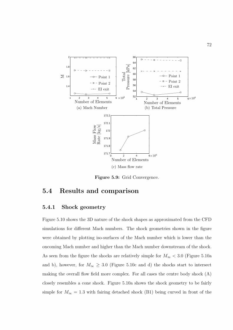
72
1 2 3 4 5 6
1.4
1.6
1.8
2
Number of Elements
M
×106
Point 1
Point 2
EI exit
(a) Mach Number
1 2 3 4 5 652
54
56
58
60
62
64
66
Number of Elements
Total
Pressure
[kPa]
×106
Point 1
Point 2
EI exit
(b) Total Pressure
0 2 4 6171.7
171.8
171.9
172
172.1
172.2
Number of Elements
MassFlow
Rate[kg/s]
×106
(c) Mass flow rate
Figure 5.9: Grid Convergence.
5.4 Results and comparison
5.4.1 Shock geometry
Figure 5.10 shows the 3D nature of the shock shapes as approximated from the CFD
simulations for different Mach numbers. The shock geometries shown in the figure
were obtained by plotting iso-surfaces of the Mach number which is lower than the
oncoming Mach number and higher than the Mach number downstream of the shock.
As seen from the figure the shocks are relatively simple for M∞ < 3.0 (Figure 5.10a
and b), however, for M∞ ≥ 3.0 (Figure 5.10c and d) the shocks start to intersect
making the overall flow field more complex. For all cases the centre body shock (A)
closely resembles a cone shock. Figure 5.10a shows the shock geometry to be fairly
simple for M∞ = 1.3 with fairing detached shock (B1) being curved in front of the
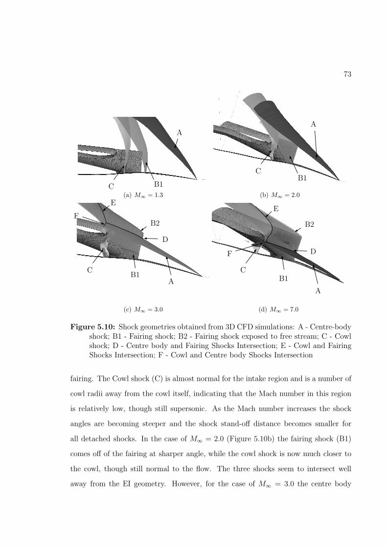
73
A
B1C(a) M∞ = 1.3
A
B1C
(b) M∞ = 2.0
A
B2
B1C
D
E
F
(c) M∞ = 3.0
A
B2
B1C
D
E
F
(d) M∞ = 7.0
Figure 5.10: Shock geometries obtained from 3D CFD simulations: A - Centre-bodyshock; B1 - Fairing shock; B2 - Fairing shock exposed to free stream; C - Cowlshock; D - Centre body and Fairing Shocks Intersection; E - Cowl and FairingShocks Intersection; F - Cowl and Centre body Shocks Intersection
fairing. The Cowl shock (C) is almost normal for the intake region and is a number of
cowl radii away from the cowl itself, indicating that the Mach number in this region
is relatively low, though still supersonic. As the Mach number increases the shock
angles are becoming steeper and the shock stand-off distance becomes smaller for
all detached shocks. In the case of M∞ = 2.0 (Figure 5.10b) the fairing shock (B1)
comes off of the fairing at sharper angle, while the cowl shock is now much closer to
the cowl, though still normal to the flow. The three shocks seem to intersect well
away from the EI geometry. However, for the case of M∞ = 3.0 the centre body
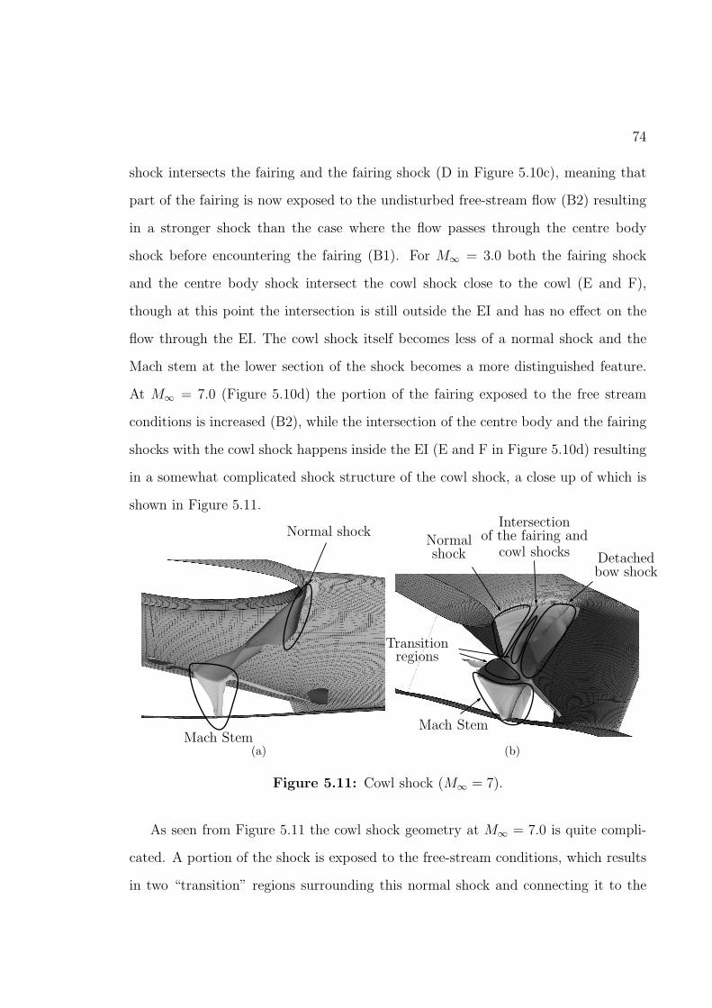
74
shock intersects the fairing and the fairing shock (D in Figure 5.10c), meaning that
part of the fairing is now exposed to the undisturbed free-stream flow (B2) resulting
in a stronger shock than the case where the flow passes through the centre body
shock before encountering the fairing (B1). For M∞ = 3.0 both the fairing shock
and the centre body shock intersect the cowl shock close to the cowl (E and F),
though at this point the intersection is still outside the EI and has no effect on the
flow through the EI. The cowl shock itself becomes less of a normal shock and the
Mach stem at the lower section of the shock becomes a more distinguished feature.
At M∞ = 7.0 (Figure 5.10d) the portion of the fairing exposed to the free stream
conditions is increased (B2), while the intersection of the centre body and the fairing
shocks with the cowl shock happens inside the EI (E and F in Figure 5.10d) resulting
in a somewhat complicated shock structure of the cowl shock, a close up of which is
shown in Figure 5.11.
Normal shock
Mach Stem(a)
Detachedbow shock
Intersectionof the fairing and
cowl shocksNormalshock
Transitionregions
Mach Stem
(b)
Figure 5.11: Cowl shock (M∞ = 7).
As seen from Figure 5.11 the cowl shock geometry at M∞ = 7.0 is quite compli-
cated. A portion of the shock is exposed to the free-stream conditions, which results
in two “transition” regions surrounding this normal shock and connecting it to the
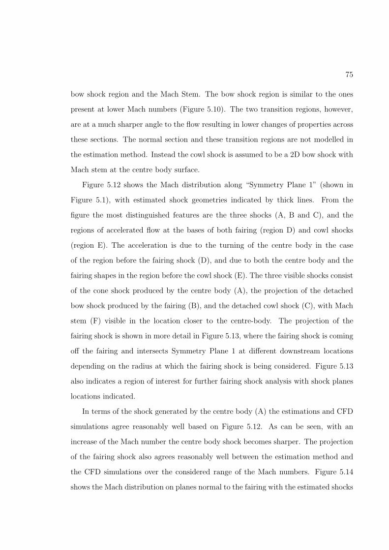
75
bow shock region and the Mach Stem. The bow shock region is similar to the ones
present at lower Mach numbers (Figure 5.10). The two transition regions, however,
are at a much sharper angle to the flow resulting in lower changes of properties across
these sections. The normal section and these transition regions are not modelled in
the estimation method. Instead the cowl shock is assumed to be a 2D bow shock with
Mach stem at the centre body surface.
Figure 5.12 shows the Mach distribution along “Symmetry Plane 1” (shown in
Figure 5.1), with estimated shock geometries indicated by thick lines. From the
figure the most distinguished features are the three shocks (A, B and C), and the
regions of accelerated flow at the bases of both fairing (region D) and cowl shocks
(region E). The acceleration is due to the turning of the centre body in the case
of the region before the fairing shock (D), and due to both the centre body and the
fairing shapes in the region before the cowl shock (E). The three visible shocks consist
of the cone shock produced by the centre body (A), the projection of the detached
bow shock produced by the fairing (B), and the detached cowl shock (C), with Mach
stem (F) visible in the location closer to the centre-body. The projection of the
fairing shock is shown in more detail in Figure 5.13, where the fairing shock is coming
off the fairing and intersects Symmetry Plane 1 at different downstream locations
depending on the radius at which the fairing shock is being considered. Figure 5.13
also indicates a region of interest for further fairing shock analysis with shock planes
locations indicated.
In terms of the shock generated by the centre body (A) the estimations and CFD
simulations agree reasonably well based on Figure 5.12. As can be seen, with an
increase of the Mach number the centre body shock becomes sharper. The projection
of the fairing shock also agrees reasonably well between the estimation method and
the CFD simulations over the considered range of the Mach numbers. Figure 5.14
shows the Mach distribution on planes normal to the fairing with the estimated shocks
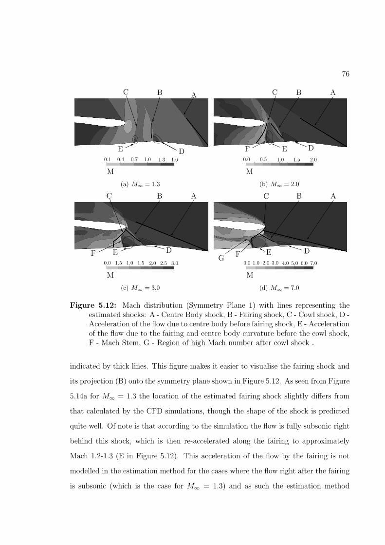
76
ABC
DE
M
0.1 0.4 0.7 1.0 1.3 1.6
(a) M∞ = 1.3
ABC
DEF
M
0.0 0.5 1.0 1.5 2.0
(b) M∞ = 2.0
ABC
DEF
M
0.0 1.5 1.0 1.5 2.0 2.5 3.0
(c) M∞ = 3.0
ABC
DEFG
M
0.0 1.0 2.0 3.0 4.0 5.0 6.0 7.0
(d) M∞ = 7.0
Figure 5.12: Mach distribution (Symmetry Plane 1) with lines representing theestimated shocks: A - Centre Body shock, B - Fairing shock, C - Cowl shock, D -Acceleration of the flow due to centre body before fairing shock, E - Accelerationof the flow due to the fairing and centre body curvature before the cowl shock,F - Mach Stem, G - Region of high Mach number after cowl shock .
indicated by thick lines. This figure makes it easier to visualise the fairing shock and
its projection (B) onto the symmetry plane shown in Figure 5.12. As seen from Figure
5.14a for M∞ = 1.3 the location of the estimated fairing shock slightly differs from
that calculated by the CFD simulations, though the shape of the shock is predicted
quite well. Of note is that according to the simulation the flow is fully subsonic right
behind this shock, which is then re-accelerated along the fairing to approximately
Mach 1.2-1.3 (E in Figure 5.12). This acceleration of the flow by the fairing is not
modelled in the estimation method for the cases where the flow right after the fairing
is subsonic (which is the case for M∞ = 1.3) and as such the estimation method
77
Fairing shock
Projection onSymmetry Plane 1
Location of Interest(Figure 5.14)
Figure 5.13: Fairing shock location and its projection to Symmetry Plane 1.
does not compute the cowl shock (hence the absence of a thick line for cowl shock
in Figure 5.14a). The cowl shock, however, is computed for cases where the flow
is supersonic after the fairing shock, as shown in the results for M∞ = 2.0 (Figure
5.12b and 5.14b). In this case the cowl shock is estimated as a detached bow shock,
while the CFD results show a Mach stem right after the region E. At M∞ = 2.0 the
geometry of the fairing shock follows the one computed by the CFD simulation very
closely in both the shock location and its shape. The same can be said about the
fairing shock shapes at M∞ = 3.0 (Figure 5.12c and 5.14c) and M∞ = 7.0 (Figure
5.12d and 5.14d). The Mach stem for these two Mach numbers is now also computed
by the estimation method, though in the case of M∞ = 3.0 the size of the Mach
stem is underestimated and it is located further downstream when compared to the
CFD results (Figure 5.14c). As was mentioned earlier, at M∞ = 7.0 both the centre
body shock and the fairing shock intersect the cowl shock producing a complicated
cowl shock geometry (Figure 5.11). Despite this, the estimation method is able to
correctly calculate the size of the Mach stem as well as the overall cowl shock shape
at Symmetry Plane 1 (Figure 5.12d).
Figure 5.12 also shows an acceleration of the flow along the centre body (D). As
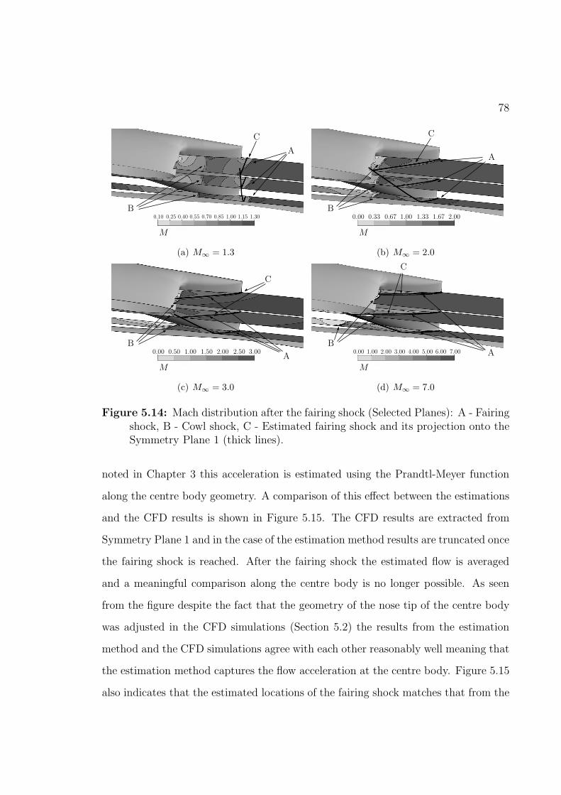
78
M
0.10 0.25 0.40 0.55 0.70 0.85 1.00 1.15 1.30
B
A
C
(a) M∞ = 1.3
M
0.00 0.33 0.67 1.00 1.33 1.67 2.00B
A
C
(b) M∞ = 2.0
M
0.00 0.50 1.00 1.50 2.00 2.50 3.00B
A
C
(c) M∞ = 3.0
M
0.00 1.00 2.00 3.00 4.00 5.00 6.00 7.00B
A
C
(d) M∞ = 7.0
Figure 5.14: Mach distribution after the fairing shock (Selected Planes): A - Fairingshock, B - Cowl shock, C - Estimated fairing shock and its projection onto theSymmetry Plane 1 (thick lines).
noted in Chapter 3 this acceleration is estimated using the Prandtl-Meyer function
along the centre body geometry. A comparison of this effect between the estimations
and the CFD results is shown in Figure 5.15. The CFD results are extracted from
Symmetry Plane 1 and in the case of the estimation method results are truncated once
the fairing shock is reached. After the fairing shock the estimated flow is averaged
and a meaningful comparison along the centre body is no longer possible. As seen
from the figure despite the fact that the geometry of the nose tip of the centre body
was adjusted in the CFD simulations (Section 5.2) the results from the estimation
method and the CFD simulations agree with each other reasonably well meaning that
the estimation method captures the flow acceleration at the centre body. Figure 5.15
also indicates that the estimated locations of the fairing shock matches that from the
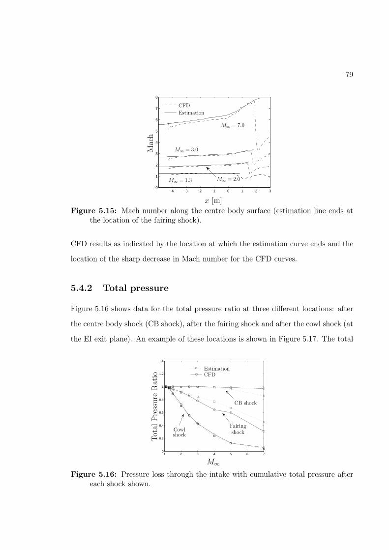
79
−4 −3 −2 −1 0 1 2 30
1
2
3
4
5
6
7
8
x [m]
Mach
CFD
Estimation
M∞ = 1.3 M∞ = 2.0
M∞ = 3.0
M∞ = 7.0
Figure 5.15: Mach number along the centre body surface (estimation line ends atthe location of the fairing shock).
CFD results as indicated by the location at which the estimation curve ends and the
location of the sharp decrease in Mach number for the CFD curves.
5.4.2 Total pressure
Figure 5.16 shows data for the total pressure ratio at three different locations: after
the centre body shock (CB shock), after the fairing shock and after the cowl shock (at
the EI exit plane). An example of these locations is shown in Figure 5.17. The total
1 2 3 4 5 6 70
0.2
0.4
0.6
0.8
1
1.2
1.4
M∞
Total
Pressure
Ratio
EstimationCFD
Cowlshock
Fairingshock
CB shock
Figure 5.16: Pressure loss through the intake with cumulative total pressure aftereach shock shown.
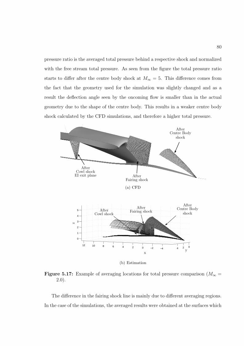
80
pressure ratio is the averaged total pressure behind a respective shock and normalized
with the free stream total pressure. As seen from the figure the total pressure ratio
starts to differ after the centre body shock at M∞ = 5. This difference comes from
the fact that the geometry used for the simulation was slightly changed and as a
result the deflection angle seen by the oncoming flow is smaller than in the actual
geometry due to the shape of the centre body. This results in a weaker centre body
shock calculated by the CFD simulations, and therefore a higher total pressure.
AfterCentre Body
shock
AfterFairing shock
AfterCowl shockEI exit plane
(a) CFD
−4−2024681012024
0
1
2
3
4
5
AfterCentre Body
shock
AfterFairing shockAfter
Cowl shock
xy
z
(b) Estimation
Figure 5.17: Example of averaging locations for total pressure comparison (M∞ =2.0).
The difference in the fairing shock line is mainly due to different averaging regions.
In the case of the simulations, the averaged results were obtained at the surfaces which
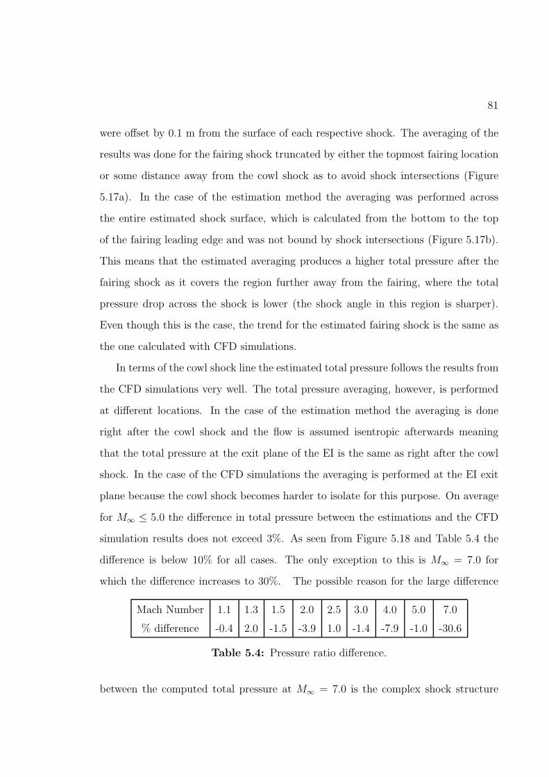
81
were offset by 0.1 m from the surface of each respective shock. The averaging of the
results was done for the fairing shock truncated by either the topmost fairing location
or some distance away from the cowl shock as to avoid shock intersections (Figure
5.17a). In the case of the estimation method the averaging was performed across
the entire estimated shock surface, which is calculated from the bottom to the top
of the fairing leading edge and was not bound by shock intersections (Figure 5.17b).
This means that the estimated averaging produces a higher total pressure after the
fairing shock as it covers the region further away from the fairing, where the total
pressure drop across the shock is lower (the shock angle in this region is sharper).
Even though this is the case, the trend for the estimated fairing shock is the same as
the one calculated with CFD simulations.
In terms of the cowl shock line the estimated total pressure follows the results from
the CFD simulations very well. The total pressure averaging, however, is performed
at different locations. In the case of the estimation method the averaging is done
right after the cowl shock and the flow is assumed isentropic afterwards meaning
that the total pressure at the exit plane of the EI is the same as right after the cowl
shock. In the case of the CFD simulations the averaging is performed at the EI exit
plane because the cowl shock becomes harder to isolate for this purpose. On average
for M∞ ≤ 5.0 the difference in total pressure between the estimations and the CFD
simulation results does not exceed 3%. As seen from Figure 5.18 and Table 5.4 the
difference is below 10% for all cases. The only exception to this is M∞ = 7.0 for
which the difference increases to 30%. The possible reason for the large difference
Mach Number 1.1 1.3 1.5 2.0 2.5 3.0 4.0 5.0 7.0
% difference -0.4 2.0 -1.5 -3.9 1.0 -1.4 -7.9 -1.0 -30.6
Table 5.4: Pressure ratio difference.
between the computed total pressure at M∞ = 7.0 is the complex shock structure
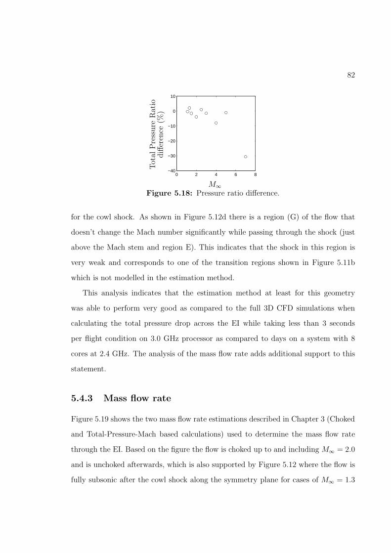
82
0 2 4 6 8−40
−30
−20
−10
0
10
M∞
Total
Pressure
Ratio
difference
(%)
Figure 5.18: Pressure ratio difference.
for the cowl shock. As shown in Figure 5.12d there is a region (G) of the flow that
doesn’t change the Mach number significantly while passing through the shock (just
above the Mach stem and region E). This indicates that the shock in this region is
very weak and corresponds to one of the transition regions shown in Figure 5.11b
which is not modelled in the estimation method.
This analysis indicates that the estimation method at least for this geometry
was able to perform very good as compared to the full 3D CFD simulations when
calculating the total pressure drop across the EI while taking less than 3 seconds
per flight condition on 3.0 GHz processor as compared to days on a system with 8
cores at 2.4 GHz. The analysis of the mass flow rate adds additional support to this
statement.
5.4.3 Mass flow rate
Figure 5.19 shows the two mass flow rate estimations described in Chapter 3 (Choked
and Total-Pressure-Mach based calculations) used to determine the mass flow rate
through the EI. Based on the figure the flow is choked up to and including M∞ = 2.0
and is unchoked afterwards, which is also supported by Figure 5.12 where the flow is
fully subsonic after the cowl shock along the symmetry plane for cases of M∞ = 1.3
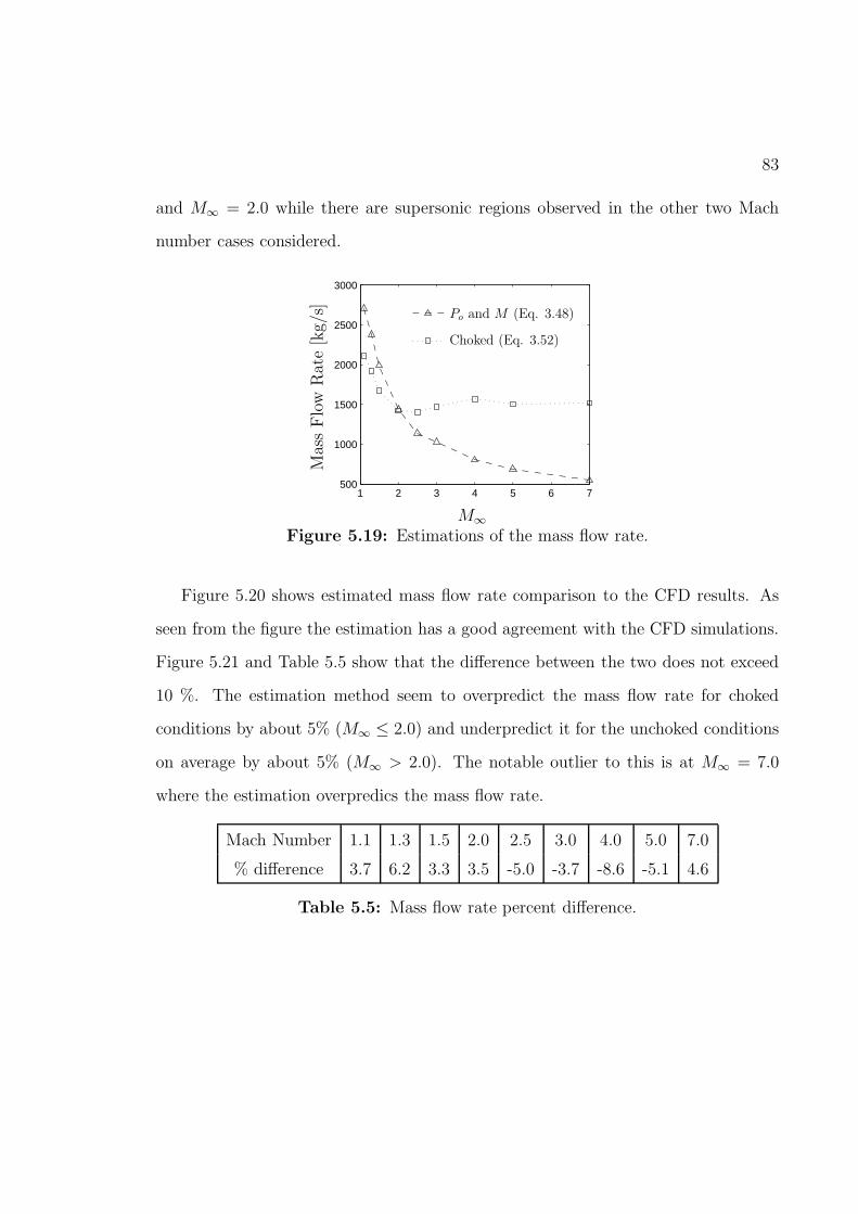
83
and M∞ = 2.0 while there are supersonic regions observed in the other two Mach
number cases considered.
1 2 3 4 5 6 7500
1000
1500
2000
2500
3000
M∞
MassFlow
Rate[kg/s] Po and M (Eq. 3.48)
Choked (Eq. 3.52)
Figure 5.19: Estimations of the mass flow rate.
Figure 5.20 shows estimated mass flow rate comparison to the CFD results. As
seen from the figure the estimation has a good agreement with the CFD simulations.
Figure 5.21 and Table 5.5 show that the difference between the two does not exceed
10 %. The estimation method seem to overpredict the mass flow rate for choked
conditions by about 5% (M∞ ≤ 2.0) and underpredict it for the unchoked conditions
on average by about 5% (M∞ > 2.0). The notable outlier to this is at M∞ = 7.0
where the estimation overpredics the mass flow rate.
Mach Number 1.1 1.3 1.5 2.0 2.5 3.0 4.0 5.0 7.0
% difference 3.7 6.2 3.3 3.5 -5.0 -3.7 -8.6 -5.1 4.6
Table 5.5: Mass flow rate percent difference.
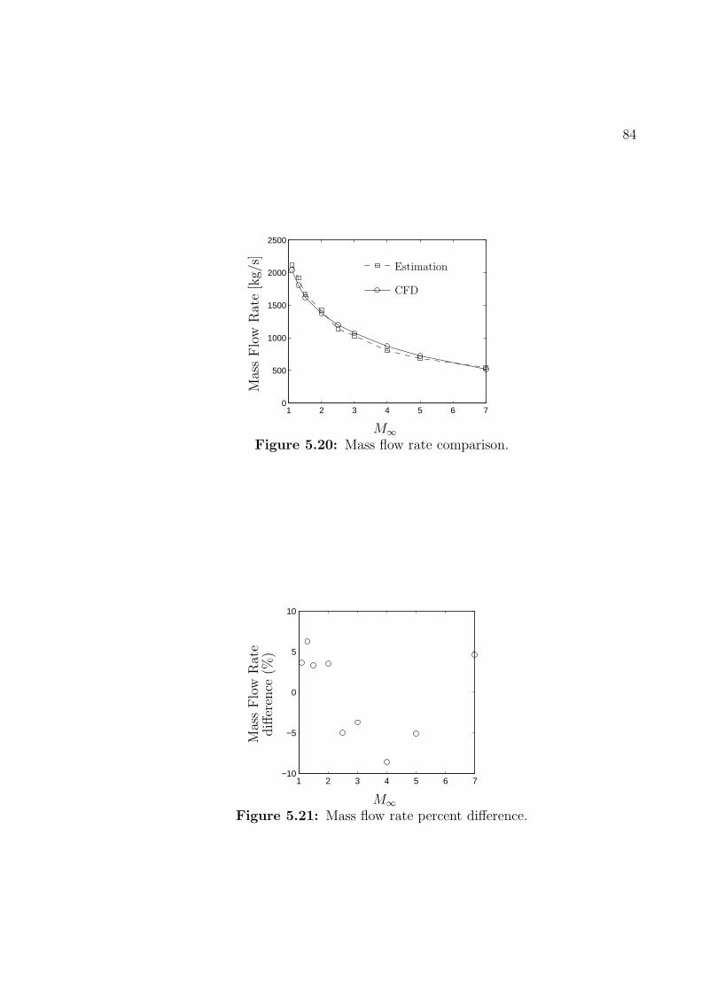
84
1 2 3 4 5 6 70
500
1000
1500
2000
2500
M∞
MassFlow
Rate[kg/s] Estimation
CFD
Figure 5.20: Mass flow rate comparison.
1 2 3 4 5 6 7−10
−5
0
5
10
M∞
MassFlow
Rate
difference
(%)
Figure 5.21: Mass flow rate percent difference.
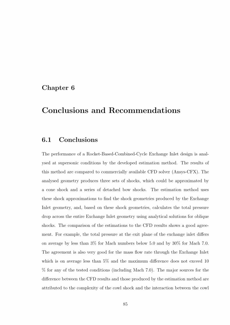
Chapter 6
Conclusions and Recommendations
6.1 Conclusions
The performance of a Rocket-Based-Combined-Cycle Exchange Inlet design is anal-
ysed at supersonic conditions by the developed estimation method. The results of
this method are compared to commercially available CFD solver (Ansys-CFX). The
analysed geometry produces three sets of shocks, which could be approximated by
a cone shock and a series of detached bow shocks. The estimation method uses
these shock approximations to find the shock geometries produced by the Exchange
Inlet geometry, and, based on these shock geometries, calculates the total pressure
drop across the entire Exchange Inlet geometry using analytical solutions for oblique
shocks. The comparison of the estimations to the CFD results shows a good agree-
ment. For example, the total pressure at the exit plane of the exchange inlet differs
on average by less than 3% for Mach numbers below 5.0 and by 30% for Mach 7.0.
The agreement is also very good for the mass flow rate through the Exchange Inlet
which is on average less than 5% and the maximum difference does not exceed 10
% for any of the tested conditions (including Mach 7.0). The major sources for the
difference between the CFD results and those produced by the estimation method are
attributed to the complexity of the cowl shock and the interaction between the cowl
85
86
and the fairing shocks which is especially true for the Mach 7.0 case, hence the large
difference.
The estimation code completes a single flight condition computation in just un-
der 3 seconds on a 3.0 GHz processor which is significantly faster than the transient
CFD simulations. In addition to that the estimation method provides with reason-
able results and as such it could be further used within an Exchange Inlet geometry
optimization algorithm.
6.2 Recommendations
The analysis of the Exchange Inlet geometry with both estimation method and CFD
simulations showed a few shortcomings of the Exchange Inlet at supersonic speeds.
The following are the recommendations for improvements in the Exchange Inlet ge-
ometry:
• The acceleration of the flow before shocks should be avoided and, if possible,
the flow should be decelerated. For supersonic flow the acceleration is caused
by expansion around concave surfaces, while deceleration is caused by convex
surfaces. The concave surfaces before the fairing and the cowl should be avoided,
or the curvature of these surfaces should be kept at a minimum.
• The leading edges should be sharp for the supersonic flow. The blunt leading
edges of the fairings and the cowl geometries cause detached bow shocks which
have a very strong shock section which in turn results in higher total pressure
drop across the Exchange Inlet. The size of this strong shock section is linearly
proportional to the radius of the leading edge, meaning the radius of the leading
edge of the fairings and the cowl should be kept to a minimum.
• The positioning of the fairing with respect to the cowl is not justified from
87
a supersonic perspective. Positioning the fairings fully within the cowl could
prevent the fairing shock from occurring, provided the flow is kept at subsonic
speed after the cowl.
The following is the list of recommendations for future work to improve the esti-
mation method:
• The testing of the performance of the method for different Exchange Inlet
geometries needs to be performed to verify the robustness of the estimation
method.
• The code would require additional modification should the fairing be moved
behind the cowl leading edge. The current version of the estimation method
stops once the properties after the cowl shock are computed. To allow for fairing
to be moved behind the cowl the flow field after the cowl shock would need to
be estimated as well.
List of References
[1] “Specific impulse.” Accessed December 03, 2012, from
http://en.wikipedia.org/wiki/Specific impulse.
[2] R. Daines and C. Segal. “Combined rocket and airbreathing propulsion systems
for space-launch applications.” Journal of Propulsion and Power 14(5), ”605–
612” (1998).
[3] S. A. Whitmore and B. J. Dunbar. “Orbital space plane: Past, present, and
future.” AIAA 2003-2718 (2003).
[4] V. Lukashevich. “Bor -1, -2, -3.” Retrieved September 15, 2012, from
http://www.buran.ru/htm/bors.htm (Russian).
[5] V. Lukashevich and I. Afanasjev. Kosmicheskie Krilja (Space Wings). LenTa
Stranstvij, Moscow, Russia (2009).
[6] J. Ray. “Pegasus launch report.” Accessed December 03, 2012, from
http://spaceflightnow.com/pegasus/hete2/status.html (2000).
[7] W. J. Escher. “Synerjet for earth/orbit propulsion - revisiting the 1966
nasa/marquardt composite (airbreathing/rocket) propulsion system study (nas7-
377).” AIAA 96-3040 (1996).
[8] Y. M. Timnat. “Recent developments in ramjets, ducted rockets and scramjets.”
Progress in Aerospace Science 27, 201–235 (1990).
[9] R. S. Fry. “A century of ramjet propulsion technology evolution.” Journal of
Propulsion and Power 20(1) (2004).
[10] R. Longstaff and A. Bond. “The skylon project.” AIAA 2011-2244 (2011).
[11] R. Daines and M. Bulman. “Computational analyses of dynamic rocket ejector
flowfields.” AIAA 96-2686 (1996).
88
89
[12] J. D. Escher and R. E. Schnurstein. “A retrospective on early cryogenic primary
rocket subsystem designs as integrated into rocket-based combined-cycle (rbcc)
engines.” Presented at the 29th Joint Propulsion Conference (Jul, 1993).
[13] F. Dykstra, A. Maree, M. Caporicci, and H. Immich. “Experimental investigation
of the thrust enhancement potential of ejector rockets.” AIAA 97-2756 (97).
[14] A. Seebass, S. Murthy, and E. Curran. “High speed flight propulsion systems.”
Progress in Astronautics and Aeronautics 137 (1991).
[15] J. J. Bertin. Hypersonic Aerothermodynamics. AIAA, Washington, USA (1994).
[16] “Gnom.” Accessed December 03, 2012, from
http://astronautix.com/lvs/gnom.htm.
[17] “Nasa’s x-43a scramjet breaks speed record.” Accessed December 03, 2012, from
http://www.nasa.gov/missions/research/x43 schedule.html (2004).
[18] D. J. Cerantola and J. Etele. “A nozzle concept to entrain atmospheric air for
ejector operation.” AIAA 2006-8089. Presented at the 14th AIAA/AHI Space
Planes and Hypersonic Systems and Technologies Conference. (2011).
[19] D. Cerantola. Rocket Nozzle Design with Ejector Effect Potential. Master’s thesis,
Carleton University (2007).
[20] T. Waung and J. Etele. “An ejector air intake design method for a novel rbcc
rocket nozzle.” AIAA (2009).
[21] T. Yuen and J. Etele. “Exchange inlet design for enhanced rbcc rocket-air mix-
ing.” AIAA (2011).
[22] G. Chorkawy. Exchange Inlet Design Optimization by Genetic Algorithm. Mas-
ter’s thesis, Carleton University (2011).
[23] ANSYS R©,Inc. ANSYS R© ICEM CFD/AI Environment, Release 12.0 Docu-
mentation (2009).
[24] ANSYS R©,Inc. ANSYS R© CFX, Release 12.0 Documentation (2009).
[25] W. Hui, J. Hu, and G. Zhao. “Gridless computation using the unified coordi-
nates.” (2004).
[26] J. Anderson. Modern Compressible Flow. McGraw-Hill Publishing Company
(1990).
90
[27] A. Ambrosio and A. Wortman. “Stagnation point shock detachment distance for
flow around spheres and cylinders.” American Rocket Society Journal 32, 281
(1962).
[28] F. S. Billig. “Shock-wave shapes around spherical & cylindrical-nosed bodies.”
Journal of Spacecraft and Rockets 4, 822–823 (1967).
[29] E. S. Love. “A reexamination of the use of simple concepts for predicting the
shape and location of detached shock waves.” National Advisory Committee for
Aeronautics NACA TN4170 (1957).
[30] G. Moretti and M. Abbett. “A time dependent computational method for blunt
body flows.” AIAA 4, 2136–2141 (1966).
[31] The MathWorks ,Inc. MATLAB, R2011b (2011).
[32] F. M. White. Fluid Mechanics. McGraw-Hill Publishing Company (1999).
[33] J. Anderson. Hypersonic and High Temperature Gas Dynamics. McGraw-Hill
Book Company (1989).
[34] E. H. Hirschel. Basic of Aerothermodynamics. Springer-Verlag, Germany (2005).
[35] M. J. Zucrow and J. D. Hoffman. Gas Dynamics: Multidimensional flow. John
Wiley and Sons, New York, USA (1976).
[36] G. Emanuel. Gasdynamics: Theory and Applications. AIAA, New York, USA
(1986).
[37] H. Versteeg and W. Malalasekera. An Introduction to Computational Fluid Dy-
namics: The Finite Volume Method. Pearson Education Limited (2007).
[38] G. Ben-Dor and K. Takayama. “The influence of the downstream pressure on the
shock wave reflection phenomenon in steady flows.” Journal of Fluid Mechanics
386, 213–232 (1999).
[39] C. Moutan. Transition between Regular Reflection and Mach Reflection in the
Dual-Solution Domain. Ph.D. thesis, California Institute of Technology (2007).
[40] H. Liepmann and A. Roshko. Elements of Gasdynamics. Galcit aeronautical
series. John Wiley & Sons (1957).
[41] “Earth atmosphere model - metric units.” Http://www.grc.nasa.gov/WWW/K-
12/airplane/atmosmet.html.

91
[42] D. Andreadis. “Scramjet engines enabling the seamless integra-
tion of air and space operations.” Retrieved April 10, 2012, from
http://www.pwrengineering.com/data.htm (2006).