Embed Size (px)
Citation preview
ROCK PHYSICS CHARACTERIZATION OF ORGANIC-RICH SHALE
FORMATIONS TO PREDICT ORGANIC PROPERTIES
A Thesis
by
BRANDON LEIGH BUSH
Submitted to the Office of Graduate Studies of
Texas A&M University
in partial fulfillment of the requirements for the degree of
MASTER OF SCIENCE
Chair of Committee, Yuefeng Sun
Committee Members, Mark Everett
Zoya Heidari
Head of Department, Rick Giardino
August 2013
Major Subject: Geophysics
Copyright 2013 Brandon Bush
ii
ABSTRACT
Hydrocarbon production from organic-rich shale formations has significantly
increased since the advent of sophisticated recovery techniques which allow for
economical production from such formations. The primary formation properties that
operators rely on to assess the economic potential of these formations are: total organic
carbon (TOC), thermal maturity, hydrocarbon saturation, porosity, mineralogy and
brittleness. In this thesis, I investigate rock physics models and methods for the possible
estimation of these formation properties of organic-rich shale formations from and well
log and seismic data.
The rock physics model applied in this research integrates Gassmann and Sun
models to predict the elastic properties of organic-rich shale formations. Sun’s model
utilizes a pore-structure parameter (PSP) which relates to the rigidity and pore structure
of the rock. The rock physics model is separated into two stages based on the
identification that organic-rich shale contains both organic and inorganic porosity.
Organic porosity contains hydrocarbon while inorganic porosity contains water; organic
porosity and associated hydrocarbon are created during the maturation of solid organic
matter. The first stage of the model incorporates the organic matter into the structural
matrix of the rock; the second stage then introduces the current total porosity into the
total rock matrix. The ideal case, studied in this paper, assumes that all porosity is
organic porosity; the parameters for each stage in the ideal case would be related and
potentially approximate to each other, simplifying the resulting nonlinear model.
iii
The modeled PSP is observed to correlate with rock properties, specifically the
TOC, hydrocarbon saturation, thermal maturity, clay volume and acoustic impedance.
Significant variation still occurs between the PSP and some rock properties, this suggests
the actual case is much more complicated than the ideal situation. A strong correlation
between the PSP and organic properties is seen as the amount of organic material
increases suggesting that higher amounts of variation with lower organic content relates
to intervals where the ideal case is not valid; the correlation is greater with respect to the
shear wave, indicating the importance of the shear wave to rock physics modeling.
Through the integration of Gassmann and Sun equations a rock physics model has been
developed which can potentially relate organic-rock properties to acoustic properties,
this correlation can greatly enhance the evaluation of organic-rich shale play
development from log analysis and possibly seismic inversion.
iv
DEDICATION
I dedicate my thesis to my grandparents and uncle who always supported me and
taught me the value of education.
v
ACKNOWLEDGEMENTS
I would like to thank my committee chair, Dr. Yuefeng Sun, and my committee
members, Dr. Everett, and Dr. Heidari for their guidance and support throughout the
course of this research.
Thanks also go to my friends and colleagues and the department faculty and staff
for making my time at Texas A&M University a great experience. I also want to extend
my gratitude to ConocoPhillips and the Berg-Hughes Center, who provided me with
Fellowship Support for my years at Texas A&M University allowing for me to focus on
my academic coursework and research. And I would especially like to thank Forest Oil
Corporation for their support in providing me with data to conduct my research.
Finally, I would greatly like to thank my family for all their support to pursue my
graduate degree.
vi
NOMENCLATURE
Pore-Structure Parameter
Shear Modulus
Porosity (Volume)
Density
Fluid Density
Poisson’s Ratio
C Compressibility
D Shear Compliance
HM Hertz-Mindlin Model
HMS Hertz-Mindlin Sun Model
HS Hashin-Shtrikman Model
Bulk Modulus of Component X
Volume of Kerogen
Modulus (Bulk or Shear)
Inverse of Modulus (Compressibility or Shear Compliance)
n Coordination Number
Dry Rock Inverse Modulus
Pore-Fill Inverse Modulus
Pe Effective Pressure
PSP Pore-Structure Parameter

vii
Compressional Velocity
Shear Velocity
viii
TABLE OF CONTENTS
Page
ABSTRACT .......................................................................................................................ii
DEDICATION .................................................................................................................. iv
ACKNOWLEDGEMENTS ............................................................................................... v
NOMENCLATURE .......................................................................................................... vi
TABLE OF CONTENTS ............................................................................................... viii
LIST OF FIGURES ............................................................................................................ x
LIST OF TABLES .......................................................................................................... xiv
1. INTRODUCTION .......................................................................................................... 1
1.1 Objectives of Study .................................................................................................. 1
1.2 Background .............................................................................................................. 3 1.2.1 Organic-Rich Shale Production ......................................................................... 3 1.2.2 Wyllie’s Time Average Equation ...................................................................... 4
1.2.3 Data ................................................................................................................... 4
1.2.4 Geology ............................................................................................................. 6
2. METHOD ..................................................................................................................... 10
2.1 Hertz-Mindlin Sun Model ...................................................................................... 10
2.2 Two-Stage Gassmann-Sun Model .......................................................................... 11 2.2.1 First Stage ........................................................................................................ 11
2.2.2 Second Stage ................................................................................................... 12 2.2.3 Organic-Rich Shales ........................................................................................ 13
2.3 Solid Matrix Modeling ........................................................................................... 15 2.4 Organic Porosity ..................................................................................................... 17 2.5 Brittleness ............................................................................................................... 18
3. INTERPRETATION .................................................................................................... 19
3.1 Shear Modulus........................................................................................................ 19 3.1.1 Lithology ......................................................................................................... 20 3.1.2 Kerogen Volume ............................................................................................. 21
3.1.3 Fluid Saturation ............................................................................................... 22 3.2 S-Wave Pore-Structure Parameter ......................................................................... 26
ix
3.2.1 Porosity ............................................................................................................ 26 3.2.2 TOC & Hydrocarbon Saturation ..................................................................... 27 3.2.3 Thermal Maturity ............................................................................................ 30 3.2.4 Lithology ......................................................................................................... 31
3.2.5 Brittleness ........................................................................................................ 35 3.3 Bulk Modulus ......................................................................................................... 36
3.3.1 Lithology ......................................................................................................... 37 3.3.2 Kerogen Volume ............................................................................................. 38 3.3.3 Fluid Saturation ............................................................................................... 40
3.4 P-Wave Pore-Structure Parameter ......................................................................... 42 3.4.1 Porosity ............................................................................................................ 45 3.4.2 TOC & Hydrocarbon Saturation ..................................................................... 45
3.4.3 Thermal Maturity ............................................................................................ 48 3.4.4 Mineralogy ...................................................................................................... 49 3.4.5 Brittleness ........................................................................................................ 55
3.5 Seismic Integration ................................................................................................. 56
4. CONCLUSIONS .......................................................................................................... 61
REFERENCES ................................................................................................................. 64
APPENDIX ...................................................................................................................... 66
x
LIST OF FIGURES
Page
Figure 1: Log Plot Showing Avalon and Wolfcamp intervals, the Bone Spring is
located between the Avalon and Upper Wolfcamp. ........................................... 7
Figure 2: Ternary matrix plot of the Avalon Shale ............................................................ 8
Figure 3: Ternary matrix plot of the Upper Wolfcamp Shale ............................................ 8
Figure 4: Ternary matrix plot of Middle and Lower Wolfcamp ........................................ 9
Figure 5: CT image showing hydrocarbon bearing porosity within organic matter
(Alfred and Vernik, 2012). ............................................................................... 18
Figure 6: Shear Modulus calculated from log data versus total porosity ......................... 19
Figure 7: Shear modulus from log data versus total porosity delineated by formation ... 20
Figure 8: Log calculated shear modulus versus total porosity for the Avalon and
Upper Wolfcamp Shales; data point color scale represents the volume of
kerogen from the GEM interpretation .............................................................. 21
Figure 9: Log calculated shear modulus versus total porosity for the Middle and
Lower Wolfcamp formations; data point color scale represents the volume
of kerogen from the GEM interpretation .......................................................... 22
Figure 10: Shear modulus versus total porosity for the Avalon Shale colored for the
water saturation from the total shale method .................................................... 23
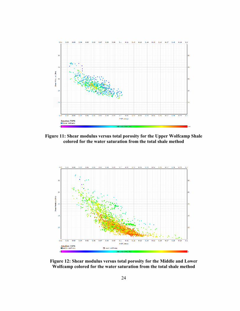
Figure 11: Shear modulus versus total porosity for the Upper Wolfcamp Shale
colored for the water saturation from the total shale method ........................... 24
Figure 12: Shear modulus versus total porosity for the Middle and Lower Wolfcamp
colored for the water saturation from the total shale method ........................... 24
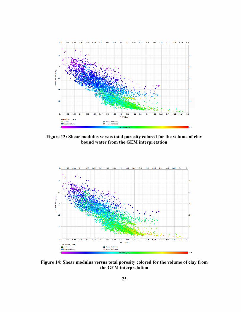
Figure 13: Shear modulus versus total porosity colored for the volume of clay bound
water from the GEM interpretation .................................................................. 25
Figure 14: Shear modulus versus total porosity colored for the volume of clay from
the GEM interpretation ..................................................................................... 25
Figure 15: Shear modulus versus total porosity colored for the S-wave pore-structure
parameter from the two stage Gassmann-Sun model ....................................... 26
xi
Figure 16: S-wave PSP versus the total porosity for the Avalon and Upper Wolfcamp . 27
Figure 17: S-wave PSP versus the hydrocarbon saturation from the total shale method
for the Avalon and Upper Wolfcamp colored for the weight percent of TOC
from the GEM interpretation ............................................................................ 28
Figure 18: S-wave PSP versus the hydrocarbon saturation data-density plot for the
Avalon and Upper Wolfcamp ........................................................................... 29
Figure 19: S-wave PSP versus the weight percent of TOC for the Avalon and Upper
Wolfcamp colored for the hydrocarbon saturation ........................................... 29
Figure 20: S-wave PSP versus the thermal maturity (Tmax) from cuttings pyrolysis
delineated for formations from the shallow Brushy Canyon to the deep
Lower Wolfcamp .............................................................................................. 30
Figure 21: Ternary matrix plot for the Avalon Shale colored for the S-wave PSP .......... 31
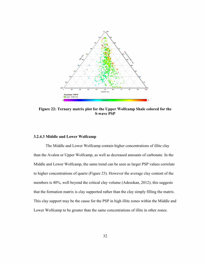
Figure 22: Ternary matrix plot for the Upper Wolfcamp Shale colored for the .............. 32
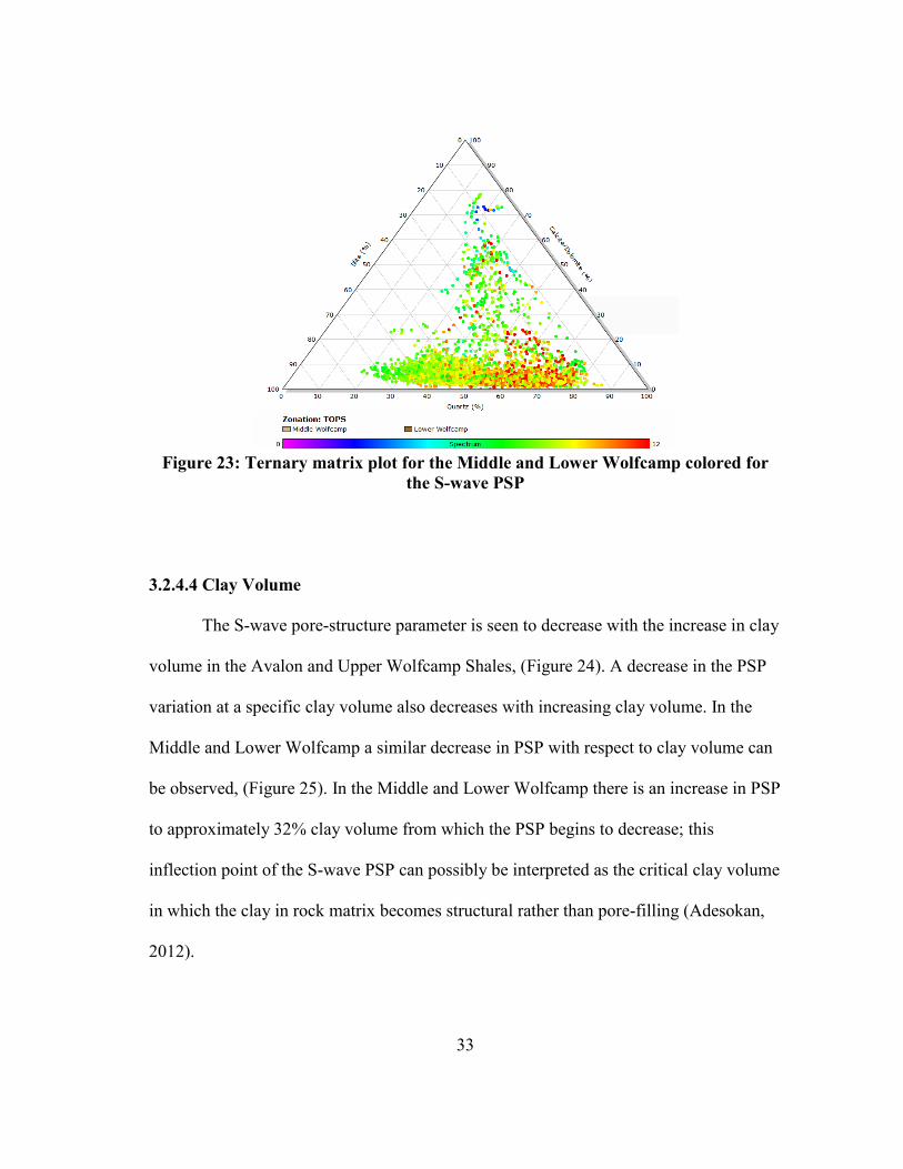
Figure 23: Ternary matrix plot for the Middle and Lower Wolfcamp colored for the
S-wave PSP ....................................................................................................... 33
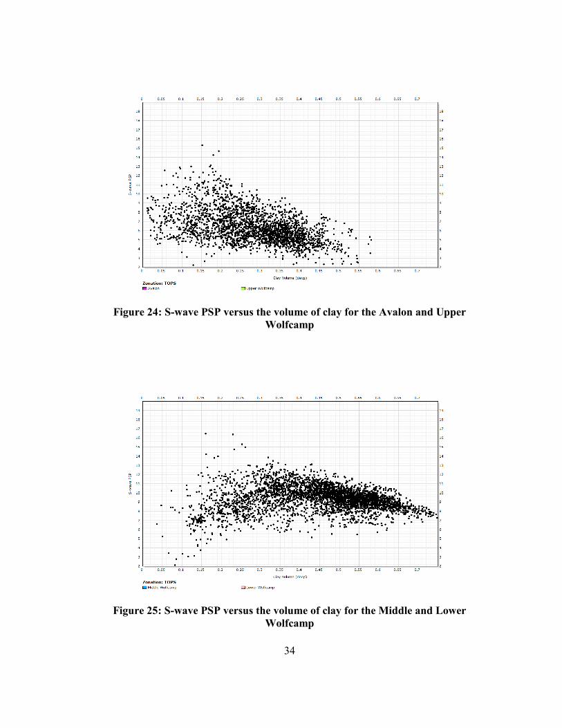
Figure 24: S-wave PSP versus the volume of clay for the Avalon and Upper
Wolfcamp ......................................................................................................... 34
Figure 25: S-wave PSP versus the volume of clay for the Middle and Lower
Wolfcamp ......................................................................................................... 34
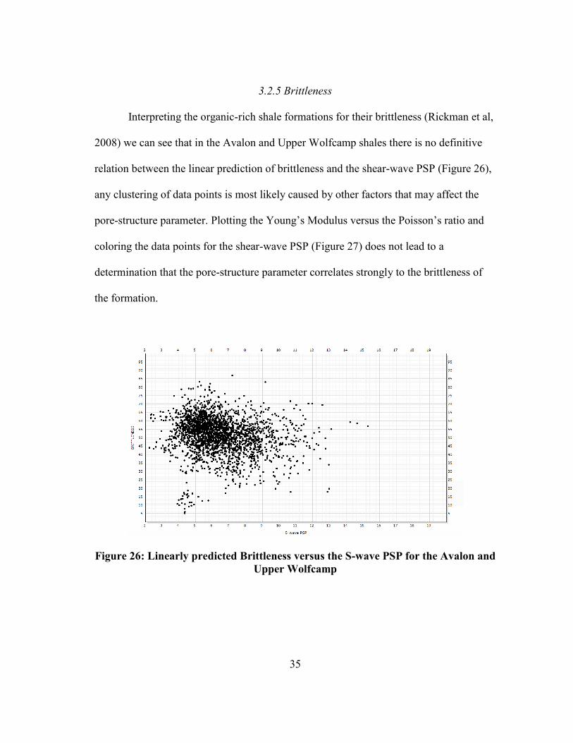
Figure 26: Linearly predicted Brittleness versus the S-wave PSP for the Avalon and
Upper Wolfcamp .............................................................................................. 35
Figure 27: Young’s Modulus versus Poisson’s Ratio for the Avalon and Upper
Wolfcamp colored for the S-wave PSP ............................................................ 36
Figure 28: Log derived bulk modulus versus the total porosity ....................................... 37
Figure 29: Bulk modulus versus the total porosity delineated for the Avalon and
Wolfcamp Group .............................................................................................. 38
Figure 30: Bulk modulus versus the total porosity for the Avalon and Upper
Wolfcamp and colored for the volume of kerogen ........................................... 39
Figure 31: Bulk modulus versus the total porosity for the Middle and Lower
Wolfcamp and colored for the volume of kerogen ........................................... 39
xii
Figure 32: Bulk modulus versus the total porosity for the Avalon and Upper
Wolfcamp colored for the water saturation ...................................................... 40
Figure 33: Bulk modulus versus the total porosity for the Middle and Lower
Wolfcamp colored for the water saturation ...................................................... 41
Figure 34: Bulk modulus versus the total porosity colored for the volume of clay
bound water ...................................................................................................... 41
Figure 35: Bulk modulus versus the total porosity colored for the volume of clay ......... 42
Figure 36: Bulk modulus versus the total porosity for the Avalon colored for the P-
wave PSP predicted from the two stage Gassmann-Sun model ....................... 43
Figure 37: Bulk modulus versus the total porosity for the Upper Wolfcamp colored
for the P-wave PSP predicted from the two stage Gassmann-Sun model ........ 44
Figure 38: Bulk modulus versus the total porosity for the Middle and Lower
Wolfcamp colored for the P-wave PSP predicted from the two stage
Gassmann-Sun model ....................................................................................... 44
Figure 39: P-wave PSP versus the total porosity for the Avalon and Upper Wolfcamp . 45
Figure 40: P-wave PSP versus the hydrocarbon saturation colored for the wt% of
TOC for the Avalon and Upper Wolfcamp ...................................................... 46
Figure 41: Data-density plot of the P-wave PSP versus the hydrocarbon saturation for
the Avalon and Upper Wolfcamp ..................................................................... 47
Figure 42: P-wave PSP versus the wt% of TOC for the Avalon and Upper Wolfcamp
colored for the hydrocarbon saturation ............................................................. 47
Figure 43: P-wave PSP versus the thermal maturity (Tmax) from cutting pyrolysis for
the logged portion of the well ........................................................................... 48
Figure 44: Ternary matrix plot of the Avalon colored for the P-wave PSP ..................... 49
Figure 45: Ternary matrix plot of the Upper Wolfcamp colored for the P-wave PSP ..... 50
Figure 46: Ternary matrix plot of the Middle Wolfcamp colored for the ........................ 51
Figure 47: Ternary matrix plot of the Lower Wolfcamp colored for the P-wave PSP .... 52
Figure 48: P-wave PSP versus the volume of clay for the Avalon .................................. 53
Figure 49: P-wave PSP versus the volume of clay for the Upper Wolfcamp .................. 53
xiii
Figure 50: P-wave PSP versus the volume of clay for the Middle Wolfcamp ................. 54
Figure 51: P-wave PSP versus the volume of clay for the Lower Wolfcamp .................. 54
Figure 52: Brittleness versus the P-wave PSP for the Avalon and Upper Wolfcamp ..... 55
Figure 53: Young’s Modulus versus Poisson’s Ratio for the Avalon and Upper
Wolfcamp colored for the P-wave PSP ............................................................ 56
Figure 54: Acoustic impedance for well log data versus the P-wave PSP for the
Avalon ............................................................................................................... 58
Figure 55: Acoustic impedance versus the S-wave PSP for the Upper Wolfcamp .......... 58
Figure 56: Acoustic impedance versus the P-wave PSP for the logged portion of the
well ................................................................................................................... 59
Figure 57: Data-density plot of the acoustic impedance versus the P-wave PSP for the
logged portion of the well ................................................................................. 59
Figure 58: S-wave PSP versus the P-wave PSP for the Avalon and Upper Wolfcamp ... 60
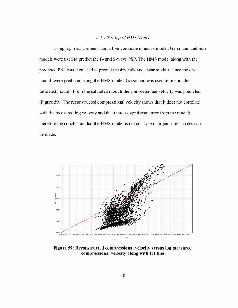
Figure 59: Reconstructed compressional velocity versus log measured compressional
velocity along with 1:1 line .............................................................................. 68
xiv
LIST OF TABLES
Page
Table 1: Acoustic rock properties used to model solid matrix moduli (Baker Hughes,
2004; Mavko et al, 2003.; Mba and Prasad, 2010; Vernik and Kachanov,
2010; Ward, 2010) ............................................................................................ 66
1
1. INTRODUCTION
Hydrocarbon production from organic-rich shale formations has significantly
increased since the advent of sophisticated recovery techniques which allow for
economical production from such formations. Some of the properties that help operators
determine whether a formation can be economically produced are: total organic carbon
(TOC), thermal maturity, hydrocarbon saturation, porosity, mineralogy and brittleness.
With the development of unconventional organic-rich shale formations, greater effort to
characterize the formations has been put forth through the collection of seismic data and
integration of borehole measurements with rock physics models.
Using various rock physics models, geoscientists are able to predict petrophysical
information through the inversion of seismic data. The Hertz-Mindlin and Sun (HMS)
rock physics model (Adesokan, 2012) was developed in a sequence of clean sand and
shaly sand formations. The HMS model was found to not be accurate in organic-rich
shale formations and therefore a two-stage rock model was used here to integrate
Gassmann (Gassmann, 1951) and Sun (Sun, 2000, Sun 2004a, Sun 2004b) models to
predict the pore-structure parameters associated with the rock (PSP). The pore-structure
parameters for P- and S-waves can then be used to potentially link formation properties,
which are integral to shale formation production, with seismic attributes so that those
properties can be predicted on field wide scale.
1.1 Objectives of Study
The purpose of this research was to apply the Hertz-Mindlin and Sun (HMS)
model to an organic-rich shale formation and then attempt to establish a relationship
2
between the model and the kerogen/TOC content of the formation using core and log
measurements. The HMS model was found to incorrectly predict the acoustic properties
of organic-rich shale formations. When the HMS model and other models (Krzikalla,
2010; Lecompte and Hursan, 2010; Vernik and Milovac, 2010) were found to not apply
to organic-rich shale formations in this study, a two stage model integrating Gassmann
and Sun models was used to predict the P- and S-wave pore-structure parameter of the
formation. The pore-structure parameter ( ) reflects the pore structure of a rock and is
believed to act as a coupling parameter from which various formation properties that
affect the pore structure of a rock may be derived. A key objective of the study was to
qualitatively determine if relationships can be established between the P-and S-wave
pore-structure parameters and the formation properties that are important to organic-rich
shale production through the use of the two-stage Gassmann-Sun model.
Another objective was to determine whether the pore-structure parameter relates
to seismic attributes and could therefore be inverted from seismic data. However, the
inversion of seismic data with the rock physics model was not be performed in this study
as there is no access to seismic data for the field in the study. It is essential to be able to
predict the organic properties of a formation, as the organic properties are important
when evaluating the economic viability of organic-rich shale formations. The inversion
of these properties from seismic surveys would greatly enhance the ability of petroleum
operating companies to economically produce from organic-rich shale formations.
3
1.2 Background
1.2.1 Organic-Rich Shale Production
Most shale reservoirs are classified as shales principally due to their physical
properties, not their lithologies. Many shale reservoirs are primarily composed of fine-
grain clastics and carbonates, producible shale reservoirs often have lower clay content
than non-reservoir shale formations. The dataset provided contains four shale formations
of interest, the Avalon and the Upper, Middle and Lower Wolfcamp shales. The Avalon
and Upper Wolfcamp Shale are primarily composed of quartz and carbonate minerals
with clay volume ranging from 5-50% in the matrix, with the majority of the clay
volumes between 18-36%. The Middle and Lower Wolfcamp are shale formations with
clay volume ranging from 10-70% with the majority of the formations containing 21-
45% clay in the matrix.
The complexity of shale reservoirs is driven by their fine-grain matrix material
which results in very low porosity (0-10%) and extremely low permeability (µDarcy-
scale). These super-low physical properties require companies to identify “sweet spots”
where reservoir properties are favorable to economic production from the reservoirs.
These sweet spots are determined by petrophysical properties such as the TOC (Total
Organic Carbon), thermal maturity, hydrocarbon saturation, porosity, mineralogy and
brittleness of the formation. A primary goal of rock physics models is to correlate these
petrophysical properties from core and well log data to geophysical methods (i.e. seismic
analysis).
4
1.2.2 Wyllie’s Time Average Equation
Previously, over-simplified models have been used to study reservoir rocks.
Wyllie et al. (1956) developed an empirical time-average model that incorporated matrix
and fluid heterogeneity in a material. Wyllie’s time-average equation is an empirically-
derived relation and does not account for pore structure or material sorting within the
rock.
1.2.3 Data
The data used for this work is from a well in the Permian Basin composed of
several organic-rich formations. The primary producible formations of interest are the
Avalon and Upper Wolfcamp Shale formations. The data includes a very comprehensive
well log package acquired by Halliburton:
Triple-Combo Logging w/Spectral Gamma Ray
Processed Full Waveform Sonic Data
GEM – Elemental Analysis Tool
The elemental analysis produced by Halliburton’s GEM tool is used to identify
the lithology of the formations and to aid in prediction of the solid matrix moduli. The
GEM elemental capture measurements have been compared to lithological results from
the core and wellbore cuttings and are found to have very similar results and therefore
can be used as the lithology log in the rock physics models. Other petrophysical
5
interpretation methods were used to compare with the GEM interpretation, when the
compared predictions were similar the GEM predictions were used in the modeling.
Numerous core experiments were performed by Weatherford on both conventional and
side-wall core:
Spectral Gamma Ray Logs from conventional cores
X-ray Refraction Analysis
X-ray Diffraction Analysis
Pyrolysis Test (Kerogen Properties)
Wellbore cuttings were analyzed by Weatherford:
Geological Logs
Geochemical Logs
Kerogen Properties (Pyrolysis)
Geological and geochemical logs from wellbore cuttings as well as XRD data
from core were used to evaluate the GEM interpretation of the matrix composition of the
formation. It was found that the GEM was not grossly misrepresenting the lithology of
the near-wellbore environment and that most differences were most likely caused by
differences in measurement techniques as well as scale differences between techniques.
Petrophysical interpretation of the logs was performed to predict the water saturation,
shale volume and mineralogy (through Techlog Quanti.Elan computation). The
petrophysical interpretation showed characteristic correlations with the GEM
interpretation, suggesting that the GEM interpretation did not produce extremely
6
questionable results and the GEM interpretation could be used in the rock physics
calculations.
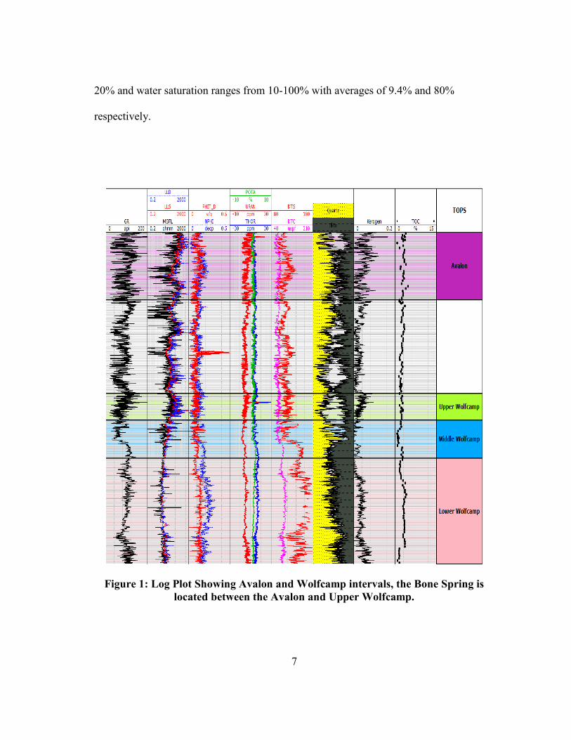
1.2.4 Geology
Several organic-rich shale formations as well as several sandstone and limestone
formations are observed in the available well data. The Avalon Shale and the Wolfcamp
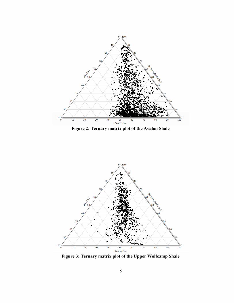
Shale are separated by the Bone Springs Group, Figure 1. The Avalon Shale (Figure 2) is
primarily composed of quartz, illite, calcite and dolomite. The ternary matrix plot for the
Avalon Shale (calcite and dolomite are combined into one component) shows that the
formation matrix is primarily carbonate material and quartz with clay comprising 5-50%
of the matrix. TOC in the Avalon Shale, from pyrolysis on cuttings, ranges from 1-5%.
Porosity ranges from 1-15% and water saturation ranges from 3-75% with averages of
6.5% and 22% respectively.
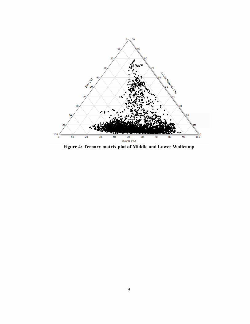
The Upper Wolfcamp Shale is the upper shale member of the Wolfcamp Group
(Figure 3); this shale has more clay and carbonates in the matrix as well as less quartz
compared to the Avalon Shale. The Avalon Shale is nearly three times thicker than the
Upper Wolfcamp Shale in the well. TOC in the Upper Wolfcamp, from pyrolysis
performed on cuttings, ranges from 1.5-3%. Porosity ranges from 2-10% and water
saturation ranges from 10-80% with averages of 6.2% and 37% respectively.
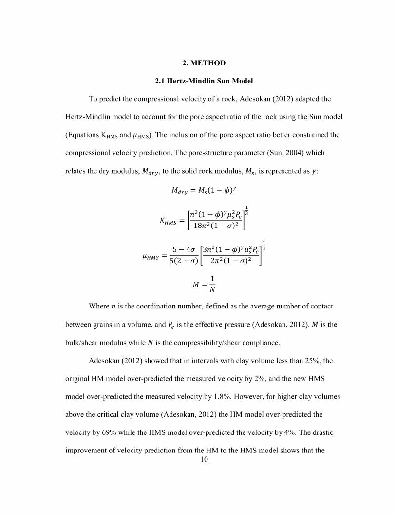
Figure 4 shows the ternary matrix plot for the Middle and Lower Wolfcamp
which are composed of primarily clay and quartz with some carbonates. The Middle and
Lower Wolfcamp are used to show lithological differences during the rock physics
modeling. TOC from cuttings pyrolysis ranges from 0.5-4%. Porosity ranges from 2.5-
7
20% and water saturation ranges from 10-100% with averages of 9.4% and 80%
respectively.
Figure 1: Log Plot Showing Avalon and Wolfcamp intervals, the Bone Spring is
located between the Avalon and Upper Wolfcamp.
8
Figure 2: Ternary matrix plot of the Avalon Shale
Figure 3: Ternary matrix plot of the Upper Wolfcamp Shale
9
Figure 4: Ternary matrix plot of Middle and Lower Wolfcamp
10
2. METHOD
2.1 Hertz-Mindlin Sun Model
To predict the compressional velocity of a rock, Adesokan (2012) adapted the
Hertz-Mindlin model to account for the pore aspect ratio of the rock using the Sun model
(Equations KHMS and HMS). The inclusion of the pore aspect ratio better constrained the
compressional velocity prediction. The pore-structure parameter (Sun, 2004) which
relates the dry modulus, , to the solid rock modulus, , is represented as :
( )
[ ( )
( )
]
( )[ ( )
( )
]
Where is the coordination number, defined as the average number of contact
between grains in a volume, and is the effective pressure (Adesokan, 2012). is the
bulk/shear modulus while is the compressibility/shear compliance.
Adesokan (2012) showed that in intervals with clay volume less than 25%, the
original HM model over-predicted the measured velocity by 2%, and the new HMS
model over-predicted the measured velocity by 1.8%. However, for higher clay volumes
above the critical clay volume (Adesokan, 2012) the HM model over-predicted the
velocity by 69% while the HMS model over-predicted the velocity by 4%. The drastic
improvement of velocity prediction from the HM to the HMS model shows that the
11
incorporation of the pore-structure parameter is important for considering the changes in
pore aspect ratio with shaly grains. The HMS model was found to not be applicable in
the organic-rich shale formations of interest in the provided dataset (Appendix).
In carbonates the pore-structure parameter can be used to identify the differing
types of porosity such as microporosity, intercrystalline, moldic and vuggy porosity
(Zhang et al., 2012). In clastic reservoirs the pore-structure parameter can be used to
predict the pore aspect ratio of the formation as well as identify fractures in conjunction
with FMI Image logs (Adesokan, 2012) which is important as pore shape is seen to
affect rock-physics modeling in shale formations (Jiang and Spikes, 2011).
2.2 Two-Stage Gassmann-Sun Model
Once the HMS model was found to not be valid in organic-rich shale formations
a two-stage model was suggested to incorporate kerogen volume into the rock
incorporating both Gassmann and Sun models. This method was developed based on a
new petrophysical model for organic-rich shales (Alfred and Vernik, 2012) in which the
rock is separated into organic and non-organic parts.
2.2.1 First Stage
The first stage of the model incorporates the deposition of organic matter,
kerogen, into the original depositional porosity through the use of Gassmann and Sun
models:
12
( )
In the Gassmann model, is the four-component solid matrix inverse modulus
(compressibility or shear compliance) from the Hill model; is the kerogen inverse
modulus; is the current volume of kerogen from the GEM interpretation; is the
dry inverse modulus with kerogen volume acting as the porosity of the rock and is
the five-component matrix incorporating kerogen into the original depositional porosity.
In the Sun model, , is the pore-structure parameter relative to the kerogen-filled
depositional porosity. In reality the pore-structure parameter relating to the kerogen
volume is very complex due to the spongy nature of kerogen. However this method is an
estimation of the potential PSP of the solid organic matter space.
2.2.2 Second Stage
The second stage of the model incorporates the creation of porosity through
maturation of the kerogen as well as water filling the non-organic porosity (Alfred and
Vernik, 2012 and Vernik and Milovac, 2011). For the shear wave, only a second Sun
model is included, however for the compressional wave a second Gassmann model is
incorporated as well. In the Sun model, is the pore structure related to the fluid filled
total porosity.
( )
13
For the shear modulus, the assumption that the dry shear modulus is equivalent to
the saturated shear modulus was used in the modeling the shear wave pore-structure
parameter:
This assumption is primarily believed to be correct in rocks with high porosity and more
spherically shaped pores. However, in very low porosity rocks it is predicted that the
fluid filled porosity does have some effect on the saturated shear modulus and greatly
increases the complexity in tight organic-rich shale formations.
2.2.3 Organic-Rich Shales
In organic-rich shales that have not expelled hydrocarbon into another formation,
the porosity of the shale is controlled by the conversion of kerogen into hydrocarbon and
porosity is created within the kerogen volume during the process. Alfred and Vernik
(2012) propose that in organic shales, all hydrocarbons are located within organic
porosity and all water is located within inorganic porosity. Within the Avalon and
Wolfcamp shales it is assumed that the separate component model is valid and that this
in turn suggests that the pore-structure parameter for the kerogen volume is
approximately equal to the PSP related to the fluid filled porosity.
The primary function of the assumption is to greatly simplify the calculations in
this research into the very ideal case. In reality the pore space is filled with both water
and hydrocarbon and therefore the pore spaces would need to be separated; also, it is
very possible that hydrocarbon may have migrated into inorganically created porosity
14
during the maturation process. These complications would require a significantly more
complex model and calculation to predict the pore-structure parameters.
2.2.3.1 Shear Wave Pore-Structure Parameter
Through combining Sun and Gassmann models and solving for the fluid filled
pore-structure parameter, a non-linear function for the parameter is derived as a function
of the kerogen-filled pore-structure parameter ( ). An iterative method is used to
solve the non-linear equation for the assumption that fluid-filled and kerogen-filled pore-
structure parameters are equivalent. This method of solving for the pore-structure
parameter was made possible by the converging nature of the two parameters to a single
value.
( )
( )( )
( ) ( )
( )
2.2.3.2 Compressional Wave Pore-Structure Parameter
The same iterative method was used to solve for the P-wave PSP that was used to
solve for the shear wave parameter. However, the modeling of the compressional wave
includes a second Gassmann model in the second stage of the rock. This causes the p-
wave PSP to be more sensitive to the fluid within the pore space and overall,
significantly more complex than the s-wave PSP.
( )( )
( ) ( )
15
( ) ( ( )( )
( ( ) ( )) )
2.3 Solid Matrix Modeling
One of the most important components of the previous rock physics models is the
modeling of the solid matrix modulus, especially in organic-rich shale formations, as
kerogen has very low acoustic properties compared to other materials (Table A-1).
Several methods were implemented to predict the solid matrix moduli for the formations.
Initially a 5-component matrix was used (quartz, calcite, dolomite, illite and kerogen)
however later a 4-component matrix (no kerogen) was used for the solid modulus. The
following models were used to predict the solid matrix moduli:
Isostrain-Voight:
∑
Isostress-Reuss:
∑
Hill:
( )
Backus Averaging (Vernik and Milovac, 2011):
(
)
16
Hashin-Shtrikman Bounding Method (Hashin and Shtrikman, 1962 and Wang and Nur,
1992):
Where:
∑
∑
And:
Where:
( )
( )
( )
( )
∑
( )
∑
( )
When comparing the various methods used to predict the solid matrix modulus of
the formation, it was found that the Hill model provided the most reliable results. The
Sun and Gassmann models were used to predict the pore-structure parameter from the
five-component matrix models and the log derived saturated moduli. It was found that
the Hill model provided the most realistic pore-structure parameter values ( )
throughout the entire well and would therefore be the method used for future
calculations.
17
2.4 Organic Porosity
Alfred and Vernik (2012) proposed a physically-consistent model for organic-
rich shales that separated the rock into two domains: organic components (solid and
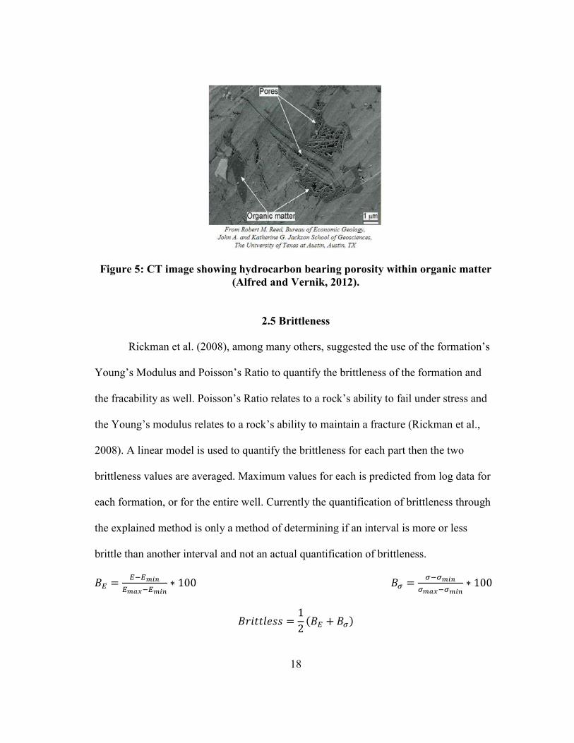
liquid) and inorganic components (matrix and water). In their model they proposed that
all hydrocarbons occurred in organically-created porosity which formed during kerogen
maturation and conversion to hydrocarbon fluids, supported by Figure 5. From their
physically-consistent model they derived a function to predict organic porosity:
( )
( ) ( )
Where is the amount of porosity in the organic domain, not the amount of
organic porosity in the total volume, as it has limits: . And is the
amount of solid organic matter in the matrix, not the entire volume. is the total
porosity of the volume. From the solid organic volume and organic porosity the total
organic volume domain is expressed as:
( )
18
Figure 5: CT image showing hydrocarbon bearing porosity within organic matter
(Alfred and Vernik, 2012).
2.5 Brittleness
Rickman et al. (2008), among many others, suggested the use of the formation’s
Young’s Modulus and Poisson’s Ratio to quantify the brittleness of the formation and
the fracability as well. Poisson’s Ratio relates to a rock’s ability to fail under stress and
the Young’s modulus relates to a rock’s ability to maintain a fracture (Rickman et al.,
2008). A linear model is used to quantify the brittleness for each part then the two
brittleness values are averaged. Maximum values for each is predicted from log data for
each formation, or for the entire well. Currently the quantification of brittleness through
the explained method is only a method of determining if an interval is more or less
brittle than another interval and not an actual quantification of brittleness.
( )
19
3. INTERPRETATION
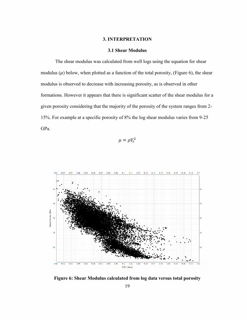
3.1 Shear Modulus
The shear modulus was calculated from well logs using the equation for shear
modulus ( ) below, when plotted as a function of the total porosity, (Figure 6), the shear
modulus is observed to decrease with increasing porosity, as is observed in other
formations. However it appears that there is significant scatter of the shear modulus for a
given porosity considering that the majority of the porosity of the system ranges from 2-
15%. For example at a specific porosity of 8% the log shear modulus varies from 9-25
GPa.
Figure 6: Shear Modulus calculated from log data versus total porosity
20
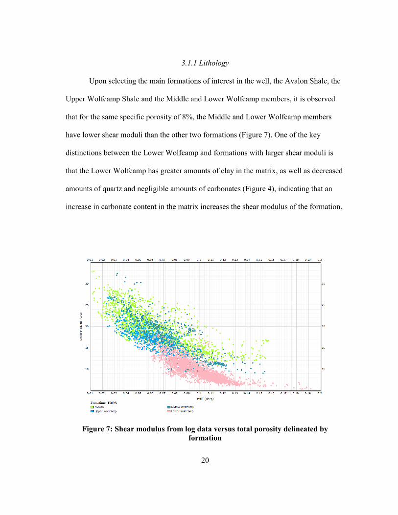
3.1.1 Lithology
Upon selecting the main formations of interest in the well, the Avalon Shale, the
Upper Wolfcamp Shale and the Middle and Lower Wolfcamp members, it is observed
that for the same specific porosity of 8%, the Middle and Lower Wolfcamp members
have lower shear moduli than the other two formations (Figure 7). One of the key
distinctions between the Lower Wolfcamp and formations with larger shear moduli is
that the Lower Wolfcamp has greater amounts of clay in the matrix, as well as decreased
amounts of quartz and negligible amounts of carbonates (Figure 4), indicating that an
increase in carbonate content in the matrix increases the shear modulus of the formation.
Figure 7: Shear modulus from log data versus total porosity delineated by
formation
21
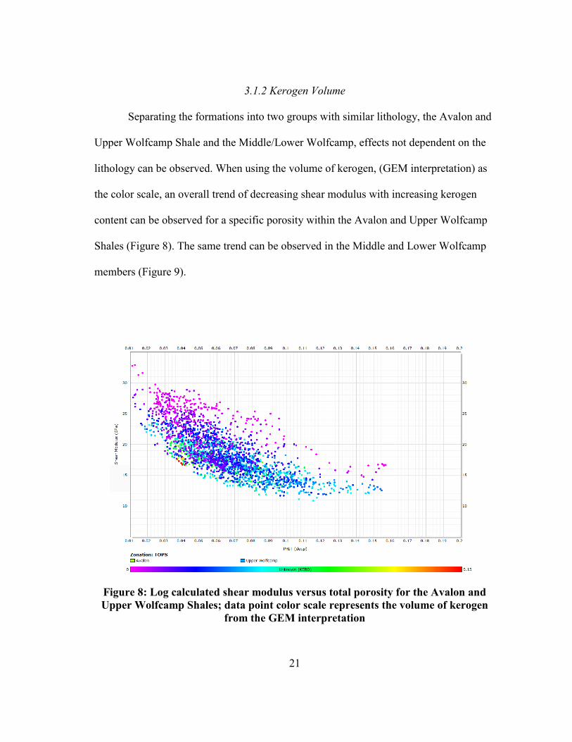
3.1.2 Kerogen Volume
Separating the formations into two groups with similar lithology, the Avalon and
Upper Wolfcamp Shale and the Middle/Lower Wolfcamp, effects not dependent on the
lithology can be observed. When using the volume of kerogen, (GEM interpretation) as
the color scale, an overall trend of decreasing shear modulus with increasing kerogen
content can be observed for a specific porosity within the Avalon and Upper Wolfcamp
Shales (Figure 8). The same trend can be observed in the Middle and Lower Wolfcamp
members (Figure 9).
Figure 8: Log calculated shear modulus versus total porosity for the Avalon and
Upper Wolfcamp Shales; data point color scale represents the volume of kerogen
from the GEM interpretation
22
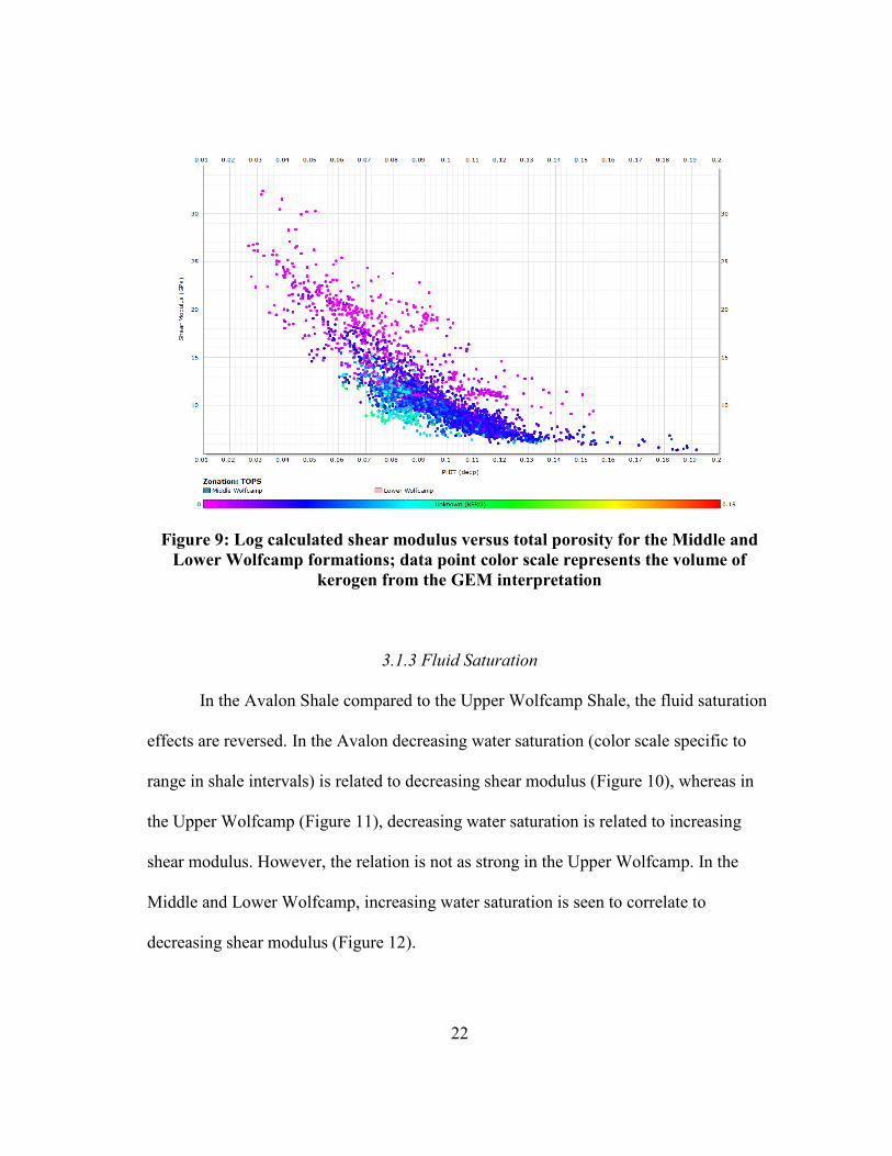
Figure 9: Log calculated shear modulus versus total porosity for the Middle and
Lower Wolfcamp formations; data point color scale represents the volume of
kerogen from the GEM interpretation
3.1.3 Fluid Saturation
In the Avalon Shale compared to the Upper Wolfcamp Shale, the fluid saturation
effects are reversed. In the Avalon decreasing water saturation (color scale specific to
range in shale intervals) is related to decreasing shear modulus (Figure 10), whereas in
the Upper Wolfcamp (Figure 11), decreasing water saturation is related to increasing
shear modulus. However, the relation is not as strong in the Upper Wolfcamp. In the
Middle and Lower Wolfcamp, increasing water saturation is seen to correlate to
decreasing shear modulus (Figure 12).
23
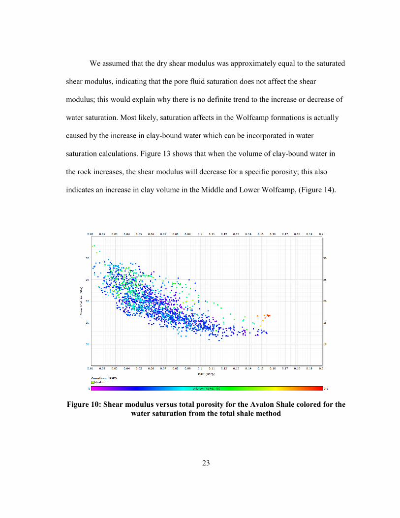
We assumed that the dry shear modulus was approximately equal to the saturated
shear modulus, indicating that the pore fluid saturation does not affect the shear
modulus; this would explain why there is no definite trend to the increase or decrease of
water saturation. Most likely, saturation affects in the Wolfcamp formations is actually
caused by the increase in clay-bound water which can be incorporated in water
saturation calculations. Figure 13 shows that when the volume of clay-bound water in
the rock increases, the shear modulus will decrease for a specific porosity; this also
indicates an increase in clay volume in the Middle and Lower Wolfcamp, (Figure 14).
Figure 10: Shear modulus versus total porosity for the Avalon Shale colored for the
water saturation from the total shale method
24
Figure 11: Shear modulus versus total porosity for the Upper Wolfcamp Shale
colored for the water saturation from the total shale method
Figure 12: Shear modulus versus total porosity for the Middle and Lower
Wolfcamp colored for the water saturation from the total shale method
25
Figure 13: Shear modulus versus total porosity colored for the volume of clay
bound water from the GEM interpretation
Figure 14: Shear modulus versus total porosity colored for the volume of clay from
the GEM interpretation
26
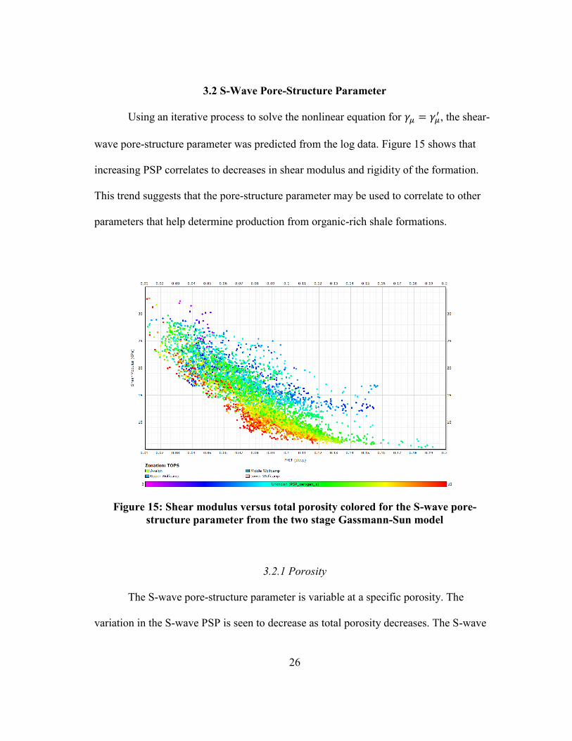
3.2 S-Wave Pore-Structure Parameter
Using an iterative process to solve the nonlinear equation for , the shear-
wave pore-structure parameter was predicted from the log data. Figure 15 shows that
increasing PSP correlates to decreases in shear modulus and rigidity of the formation.
This trend suggests that the pore-structure parameter may be used to correlate to other
parameters that help determine production from organic-rich shale formations.
Figure 15: Shear modulus versus total porosity colored for the S-wave pore-
structure parameter from the two stage Gassmann-Sun model
3.2.1 Porosity
The S-wave pore-structure parameter is variable at a specific porosity. The
variation in the S-wave PSP is seen to decrease as total porosity decreases. The S-wave
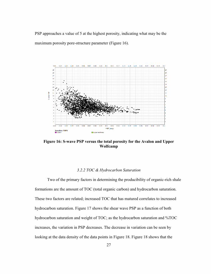
27
PSP approaches a value of 5 at the highest porosity, indicating what may be the
maximum porosity pore-structure parameter (Figure 16).
Figure 16: S-wave PSP versus the total porosity for the Avalon and Upper
Wolfcamp
3.2.2 TOC & Hydrocarbon Saturation
Two of the primary factors in determining the producibility of organic-rich shale
formations are the amount of TOC (total organic carbon) and hydrocarbon saturation.
These two factors are related; increased TOC that has matured correlates to increased
hydrocarbon saturation. Figure 17 shows the shear wave PSP as a function of both
hydrocarbon saturation and weight of TOC; as the hydrocarbon saturation and %TOC
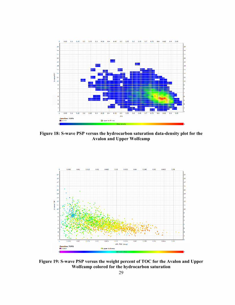
increases, the variation in PSP decreases. The decrease in variation can be seen by
looking at the data density of the data points in Figure 18. Figure 18 shows that the
28
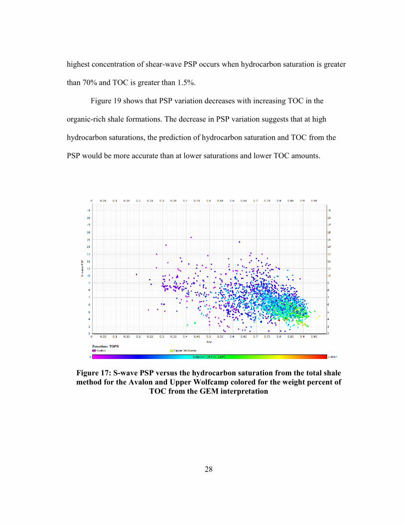
highest concentration of shear-wave PSP occurs when hydrocarbon saturation is greater
than 70% and TOC is greater than 1.5%.
Figure 19 shows that PSP variation decreases with increasing TOC in the
organic-rich shale formations. The decrease in PSP variation suggests that at high
hydrocarbon saturations, the prediction of hydrocarbon saturation and TOC from the
PSP would be more accurate than at lower saturations and lower TOC amounts.
Figure 17: S-wave PSP versus the hydrocarbon saturation from the total shale
method for the Avalon and Upper Wolfcamp colored for the weight percent of
TOC from the GEM interpretation
29
Figure 18: S-wave PSP versus the hydrocarbon saturation data-density plot for the
Avalon and Upper Wolfcamp
Figure 19: S-wave PSP versus the weight percent of TOC for the Avalon and Upper
Wolfcamp colored for the hydrocarbon saturation
30
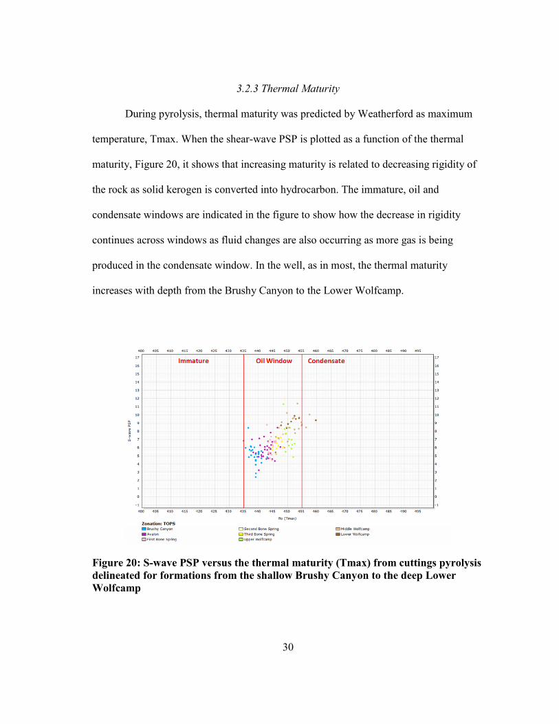
3.2.3 Thermal Maturity
During pyrolysis, thermal maturity was predicted by Weatherford as maximum
temperature, Tmax. When the shear-wave PSP is plotted as a function of the thermal
maturity, Figure 20, it shows that increasing maturity is related to decreasing rigidity of
the rock as solid kerogen is converted into hydrocarbon. The immature, oil and
condensate windows are indicated in the figure to show how the decrease in rigidity
continues across windows as fluid changes are also occurring as more gas is being
produced in the condensate window. In the well, as in most, the thermal maturity
increases with depth from the Brushy Canyon to the Lower Wolfcamp.
Figure 20: S-wave PSP versus the thermal maturity (Tmax) from cuttings pyrolysis
delineated for formations from the shallow Brushy Canyon to the deep Lower
Wolfcamp
31
3.2.4 Lithology
3.2.4.1 Avalon
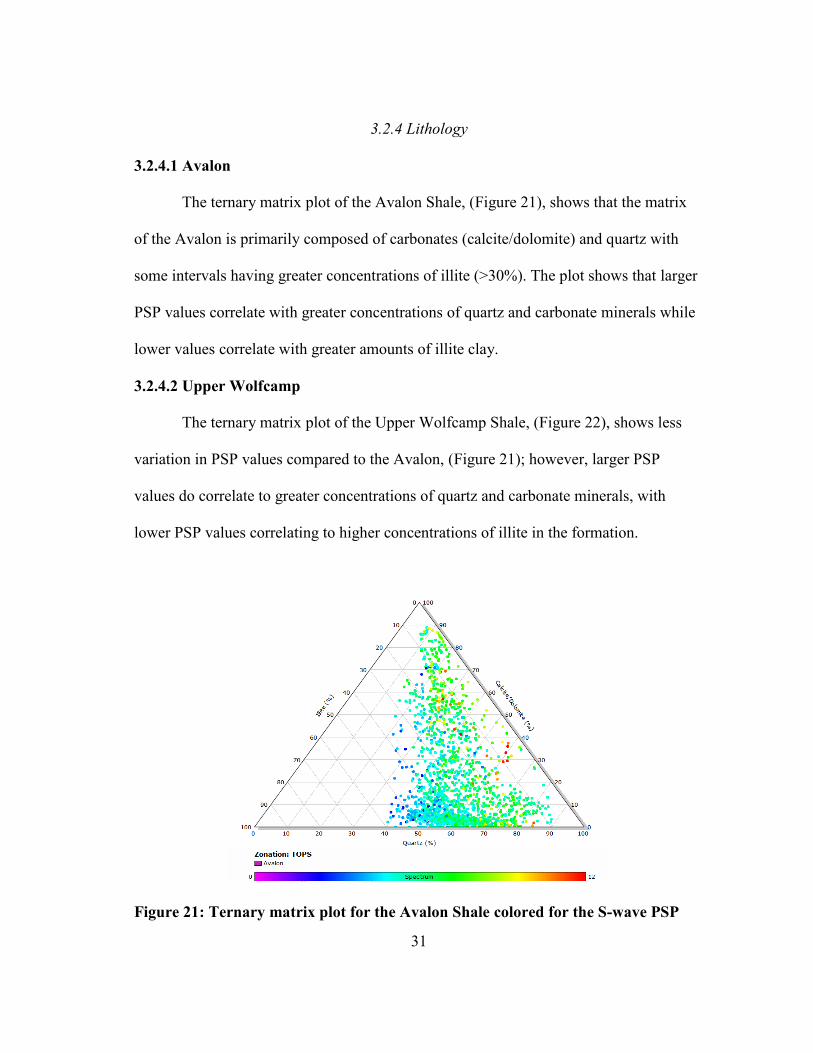
The ternary matrix plot of the Avalon Shale, (Figure 21), shows that the matrix
of the Avalon is primarily composed of carbonates (calcite/dolomite) and quartz with
some intervals having greater concentrations of illite (>30%). The plot shows that larger
PSP values correlate with greater concentrations of quartz and carbonate minerals while
lower values correlate with greater amounts of illite clay.
3.2.4.2 Upper Wolfcamp
The ternary matrix plot of the Upper Wolfcamp Shale, (Figure 22), shows less
variation in PSP values compared to the Avalon, (Figure 21); however, larger PSP
values do correlate to greater concentrations of quartz and carbonate minerals, with
lower PSP values correlating to higher concentrations of illite in the formation.
Figure 21: Ternary matrix plot for the Avalon Shale colored for the S-wave PSP
32
Figure 22: Ternary matrix plot for the Upper Wolfcamp Shale colored for the
S-wave PSP
3.2.4.3 Middle and Lower Wolfcamp
The Middle and Lower Wolfcamp contain higher concentrations of illite clay
than the Avalon or Upper Wolfcamp, as well as decreased amounts of carbonate. In the
Middle and Lower Wolfcamp, the same trend can be seen as larger PSP values correlate
to higher concentrations of quartz (Figure 23). However the average clay content of the
members is 40%, well beyond the critical clay volume (Adesokan, 2012); this suggests
that the formation matrix is clay supported rather than the clay simply filling the matrix.
This clay support may be the cause for the PSP in high illite zones within the Middle and
Lower Wolfcamp to be greater than the same concentrations of illite in other zones.
33
Figure 23: Ternary matrix plot for the Middle and Lower Wolfcamp colored for
the S-wave PSP
3.2.4.4 Clay Volume
The S-wave pore-structure parameter is seen to decrease with the increase in clay
volume in the Avalon and Upper Wolfcamp Shales, (Figure 24). A decrease in the PSP
variation at a specific clay volume also decreases with increasing clay volume. In the
Middle and Lower Wolfcamp a similar decrease in PSP with respect to clay volume can
be observed, (Figure 25). In the Middle and Lower Wolfcamp there is an increase in PSP
to approximately 32% clay volume from which the PSP begins to decrease; this
inflection point of the S-wave PSP can possibly be interpreted as the critical clay volume
in which the clay in rock matrix becomes structural rather than pore-filling (Adesokan,
2012).
34
Figure 24: S-wave PSP versus the volume of clay for the Avalon and Upper
Wolfcamp
Figure 25: S-wave PSP versus the volume of clay for the Middle and Lower
Wolfcamp
35
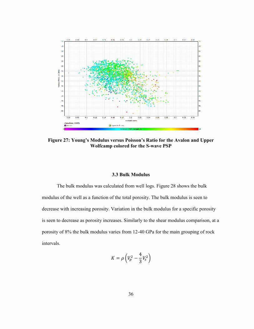
3.2.5 Brittleness
Interpreting the organic-rich shale formations for their brittleness (Rickman et al,
2008) we can see that in the Avalon and Upper Wolfcamp shales there is no definitive
relation between the linear prediction of brittleness and the shear-wave PSP (Figure 26),
any clustering of data points is most likely caused by other factors that may affect the
pore-structure parameter. Plotting the Young’s Modulus versus the Poisson’s ratio and
coloring the data points for the shear-wave PSP (Figure 27) does not lead to a
determination that the pore-structure parameter correlates strongly to the brittleness of
the formation.
Figure 26: Linearly predicted Brittleness versus the S-wave PSP for the Avalon and
Upper Wolfcamp
36
Figure 27: Young’s Modulus versus Poisson’s Ratio for the Avalon and Upper
Wolfcamp colored for the S-wave PSP
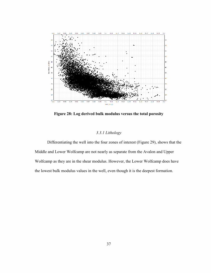
3.3 Bulk Modulus
The bulk modulus was calculated from well logs. Figure 28 shows the bulk
modulus of the well as a function of the total porosity. The bulk modulus is seen to
decrease with increasing porosity. Variation in the bulk modulus for a specific porosity
is seen to decrease as porosity increases. Similarly to the shear modulus comparison, at a
porosity of 8% the bulk modulus varies from 12-40 GPa for the main grouping of rock
intervals.
(
)
37
Figure 28: Log derived bulk modulus versus the total porosity
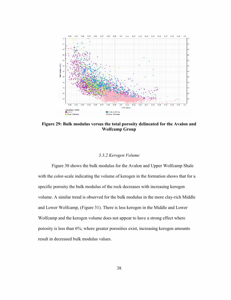
3.3.1 Lithology
Differentiating the well into the four zones of interest (Figure 29), shows that the
Middle and Lower Wolfcamp are not nearly as separate from the Avalon and Upper
Wolfcamp as they are in the shear modulus. However, the Lower Wolfcamp does have
the lowest bulk modulus values in the well, even though it is the deepest formation.
38
Figure 29: Bulk modulus versus the total porosity delineated for the Avalon and
Wolfcamp Group
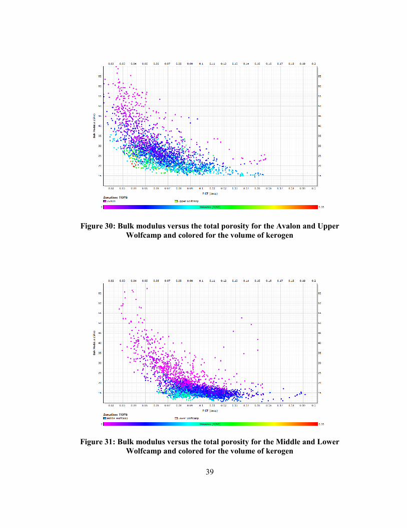
3.3.2 Kerogen Volume
Figure 30 shows the bulk modulus for the Avalon and Upper Wolfcamp Shale
with the color-scale indicating the volume of kerogen in the formation shows that for a
specific porosity the bulk modulus of the rock decreases with increasing kerogen
volume. A similar trend is observed for the bulk modulus in the more clay-rich Middle
and Lower Wolfcamp, (Figure 31). There is less kerogen in the Middle and Lower
Wolfcamp and the kerogen volume does not appear to have a strong effect where
porosity is less than 6%; where greater porosities exist, increasing kerogen amounts
result in decreased bulk modulus values.
39
Figure 30: Bulk modulus versus the total porosity for the Avalon and Upper
Wolfcamp and colored for the volume of kerogen
Figure 31: Bulk modulus versus the total porosity for the Middle and Lower
Wolfcamp and colored for the volume of kerogen
40
3.3.3 Fluid Saturation
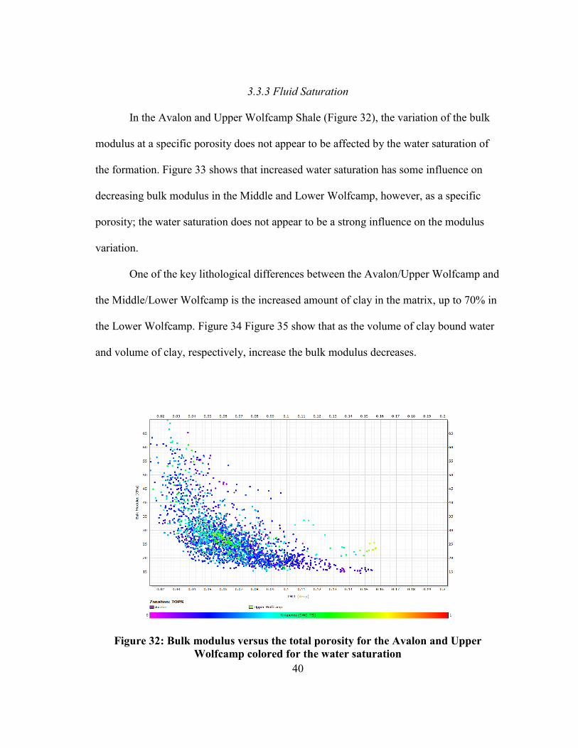
In the Avalon and Upper Wolfcamp Shale (Figure 32), the variation of the bulk
modulus at a specific porosity does not appear to be affected by the water saturation of
the formation. Figure 33 shows that increased water saturation has some influence on
decreasing bulk modulus in the Middle and Lower Wolfcamp, however, as a specific
porosity; the water saturation does not appear to be a strong influence on the modulus
variation.
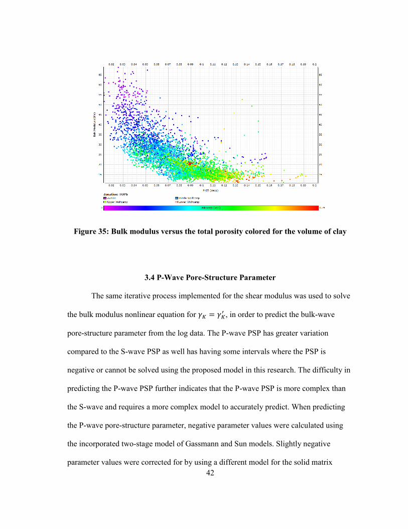
One of the key lithological differences between the Avalon/Upper Wolfcamp and
the Middle/Lower Wolfcamp is the increased amount of clay in the matrix, up to 70% in
the Lower Wolfcamp. Figure 34 Figure 35 show that as the volume of clay bound water
and volume of clay, respectively, increase the bulk modulus decreases.
Figure 32: Bulk modulus versus the total porosity for the Avalon and Upper
Wolfcamp colored for the water saturation

41
Figure 33: Bulk modulus versus the total porosity for the Middle and Lower
Wolfcamp colored for the water saturation
Figure 34: Bulk modulus versus the total porosity colored for the volume of clay
bound water
42
Figure 35: Bulk modulus versus the total porosity colored for the volume of clay
3.4 P-Wave Pore-Structure Parameter
The same iterative process implemented for the shear modulus was used to solve
the bulk modulus nonlinear equation for , in order to predict the bulk-wave
pore-structure parameter from the log data. The P-wave PSP has greater variation
compared to the S-wave PSP as well has having some intervals where the PSP is
negative or cannot be solved using the proposed model in this research. The difficulty in
predicting the P-wave PSP further indicates that the P-wave PSP is more complex than
the S-wave and requires a more complex model to accurately predict. When predicting
the P-wave pore-structure parameter, negative parameter values were calculated using
the incorporated two-stage model of Gassmann and Sun models. Slightly negative
parameter values were corrected for by using a different model for the solid matrix
43
modulus (using Voight’s model instead of Hill). A merged final PSP based on the Hill
model for the majority of data points as well as Voight’s model where Hill’s model
produced negative PSP values. However in some intervals, extremely large negative
values were calculated, especially in the Middle and Lower Wolfcamp where platy
crack-like pores exist due to the clay supported matrix of the formations.
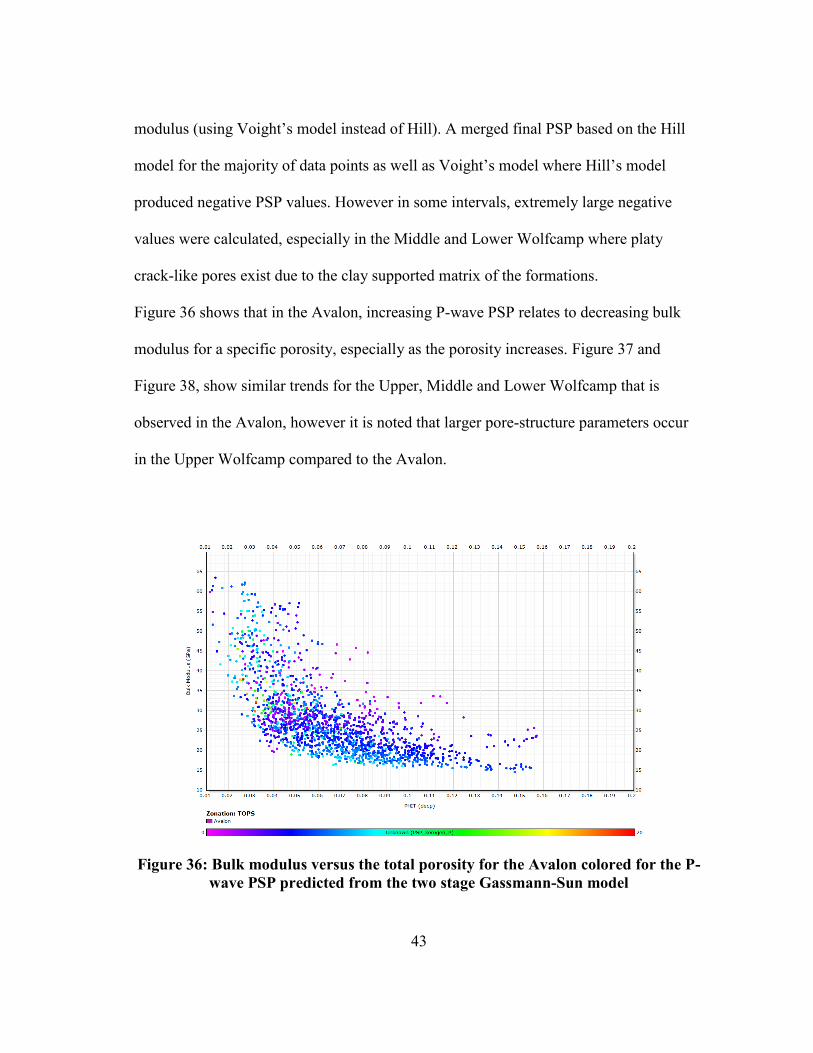
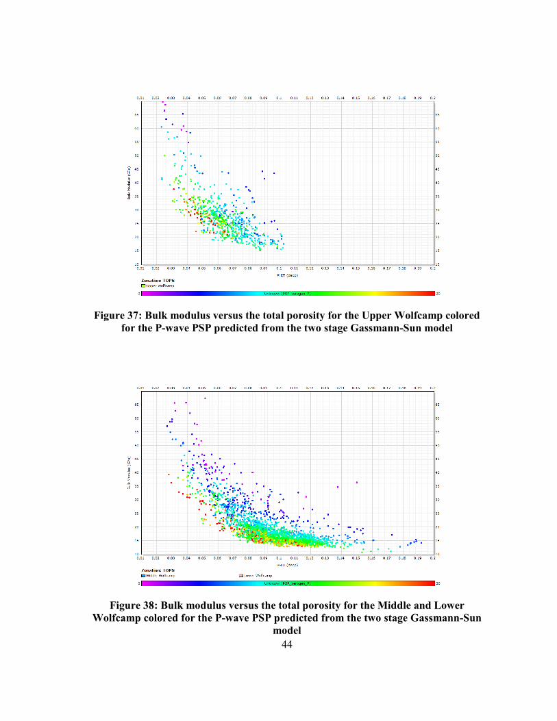
Figure 36 shows that in the Avalon, increasing P-wave PSP relates to decreasing bulk
modulus for a specific porosity, especially as the porosity increases. Figure 37 and
Figure 38, show similar trends for the Upper, Middle and Lower Wolfcamp that is
observed in the Avalon, however it is noted that larger pore-structure parameters occur
in the Upper Wolfcamp compared to the Avalon.
Figure 36: Bulk modulus versus the total porosity for the Avalon colored for the P-
wave PSP predicted from the two stage Gassmann-Sun model
44
Figure 37: Bulk modulus versus the total porosity for the Upper Wolfcamp colored
for the P-wave PSP predicted from the two stage Gassmann-Sun model
Figure 38: Bulk modulus versus the total porosity for the Middle and Lower
Wolfcamp colored for the P-wave PSP predicted from the two stage Gassmann-Sun
model
45
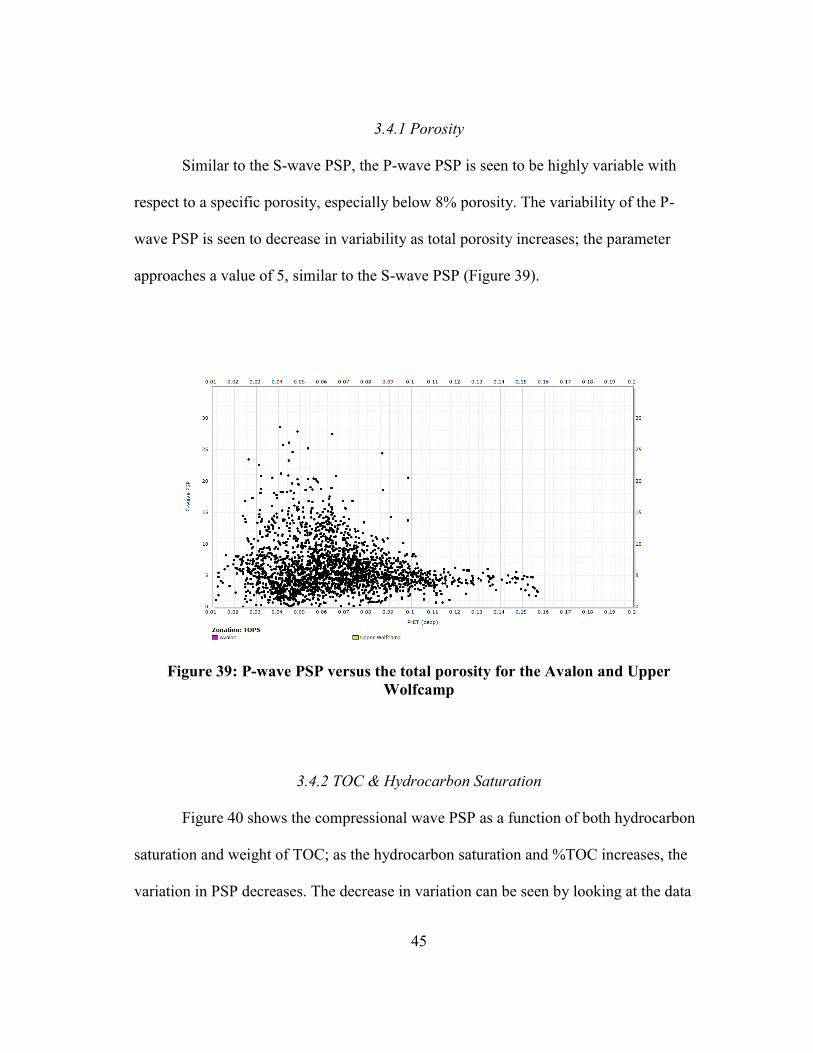
3.4.1 Porosity
Similar to the S-wave PSP, the P-wave PSP is seen to be highly variable with
respect to a specific porosity, especially below 8% porosity. The variability of the P-
wave PSP is seen to decrease in variability as total porosity increases; the parameter
approaches a value of 5, similar to the S-wave PSP (Figure 39).
Figure 39: P-wave PSP versus the total porosity for the Avalon and Upper
Wolfcamp
3.4.2 TOC & Hydrocarbon Saturation
Figure 40 shows the compressional wave PSP as a function of both hydrocarbon
saturation and weight of TOC; as the hydrocarbon saturation and %TOC increases, the
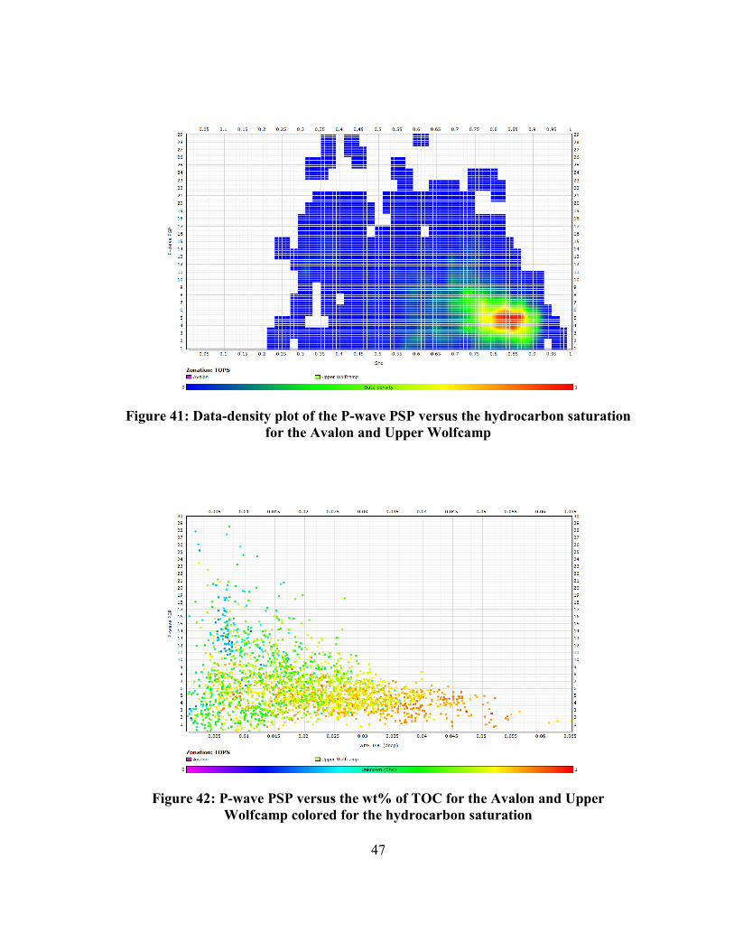
variation in PSP decreases. The decrease in variation can be seen by looking at the data
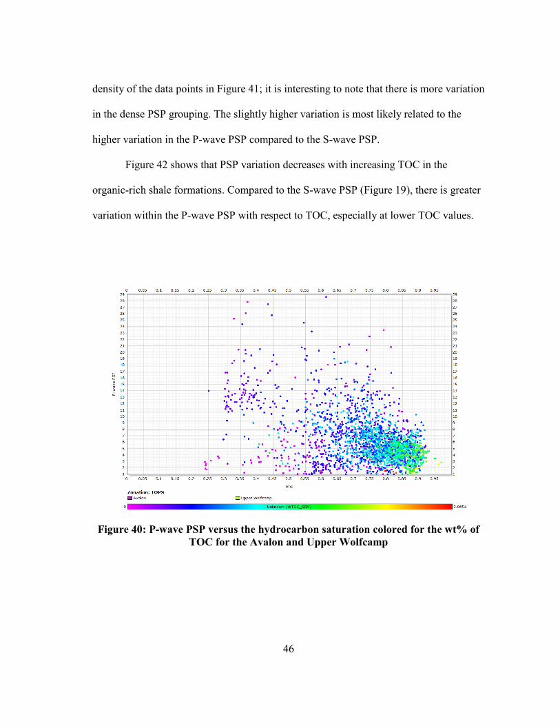
46
density of the data points in Figure 41; it is interesting to note that there is more variation
in the dense PSP grouping. The slightly higher variation is most likely related to the
higher variation in the P-wave PSP compared to the S-wave PSP.
Figure 42 shows that PSP variation decreases with increasing TOC in the
organic-rich shale formations. Compared to the S-wave PSP (Figure 19), there is greater
variation within the P-wave PSP with respect to TOC, especially at lower TOC values.
Figure 40: P-wave PSP versus the hydrocarbon saturation colored for the wt% of
TOC for the Avalon and Upper Wolfcamp
47
Figure 41: Data-density plot of the P-wave PSP versus the hydrocarbon saturation
for the Avalon and Upper Wolfcamp
Figure 42: P-wave PSP versus the wt% of TOC for the Avalon and Upper
Wolfcamp colored for the hydrocarbon saturation
48
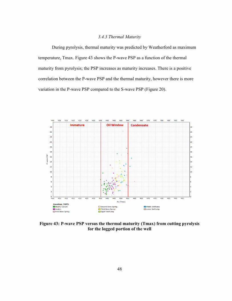
3.4.3 Thermal Maturity
During pyrolysis, thermal maturity was predicted by Weatherford as maximum
temperature, Tmax. Figure 43 shows the P-wave PSP as a function of the thermal
maturity from pyrolysis; the PSP increases as maturity increases. There is a positive
correlation between the P-wave PSP and the thermal maturity, however there is more
variation in the P-wave PSP compared to the S-wave PSP (Figure 20).
Figure 43: P-wave PSP versus the thermal maturity (Tmax) from cutting pyrolysis
for the logged portion of the well
49
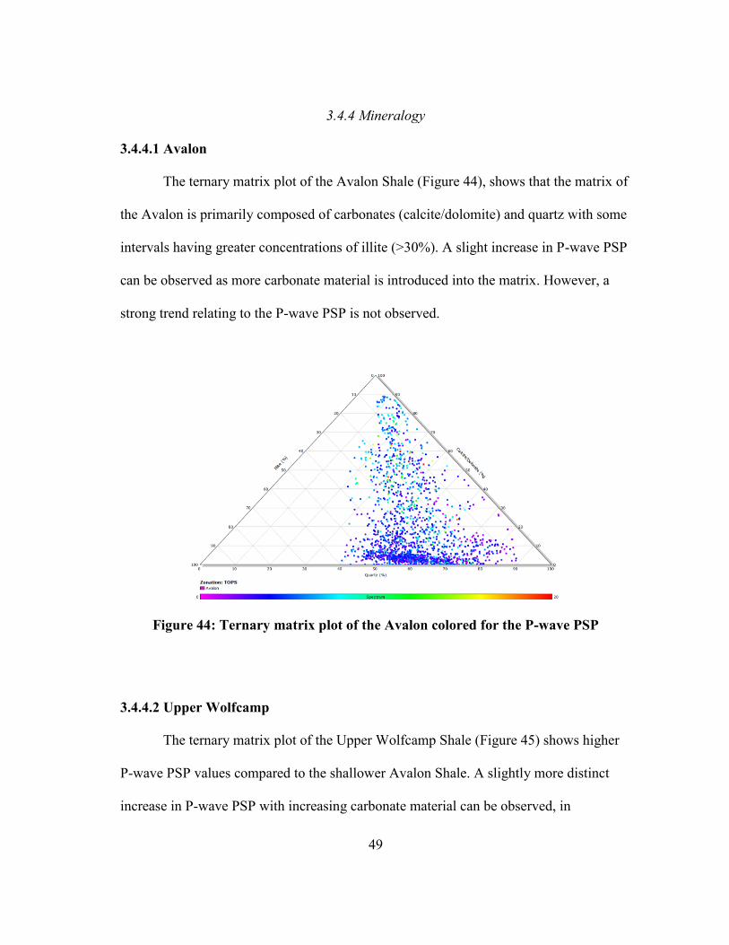
3.4.4 Mineralogy
3.4.4.1 Avalon
The ternary matrix plot of the Avalon Shale (Figure 44), shows that the matrix of
the Avalon is primarily composed of carbonates (calcite/dolomite) and quartz with some
intervals having greater concentrations of illite (>30%). A slight increase in P-wave PSP
can be observed as more carbonate material is introduced into the matrix. However, a
strong trend relating to the P-wave PSP is not observed.
Figure 44: Ternary matrix plot of the Avalon colored for the P-wave PSP
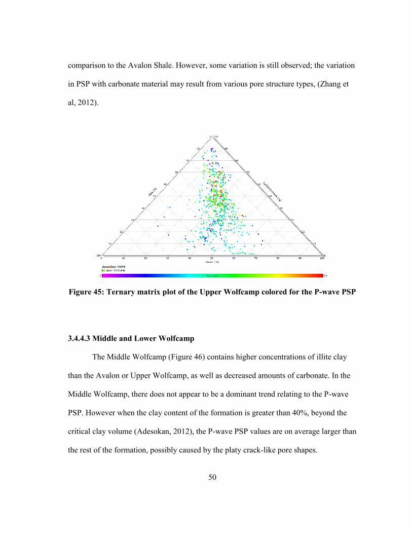
3.4.4.2 Upper Wolfcamp
The ternary matrix plot of the Upper Wolfcamp Shale (Figure 45) shows higher
P-wave PSP values compared to the shallower Avalon Shale. A slightly more distinct
increase in P-wave PSP with increasing carbonate material can be observed, in
50
comparison to the Avalon Shale. However, some variation is still observed; the variation
in PSP with carbonate material may result from various pore structure types, (Zhang et
al, 2012).
Figure 45: Ternary matrix plot of the Upper Wolfcamp colored for the P-wave PSP
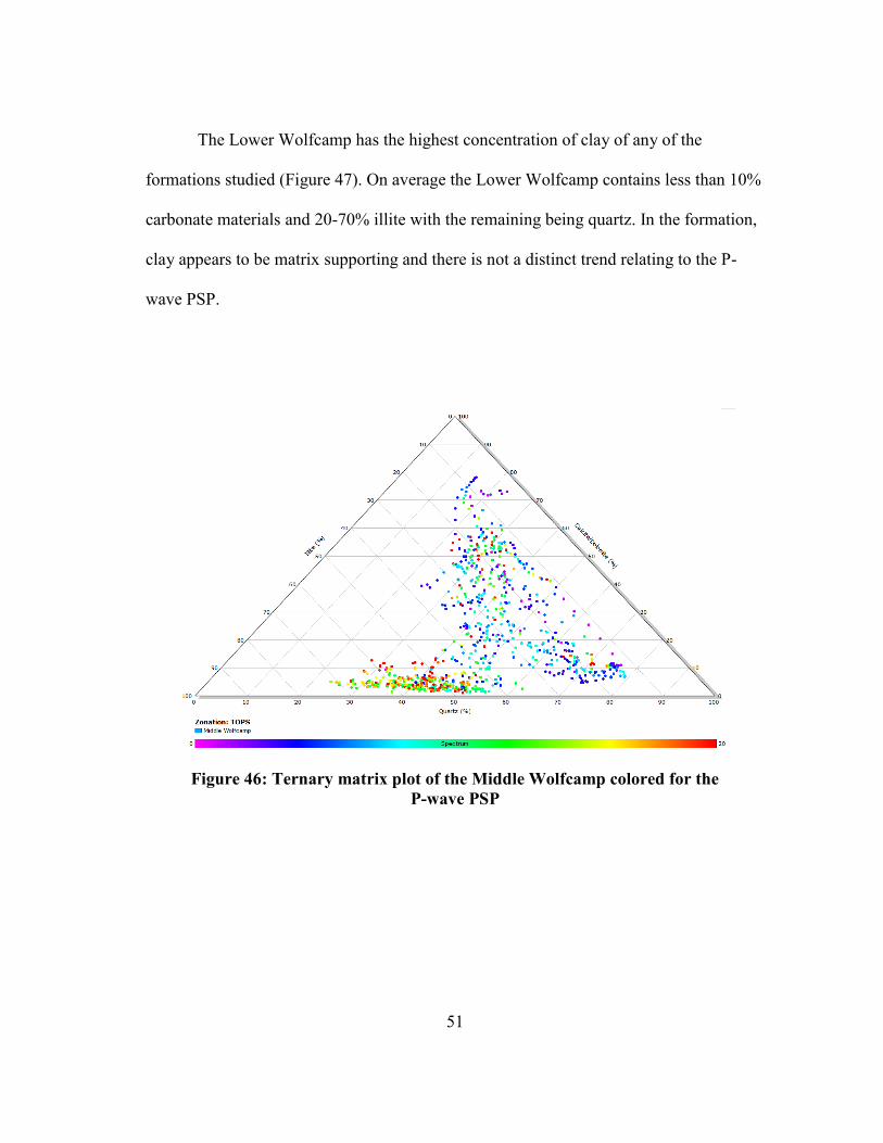
3.4.4.3 Middle and Lower Wolfcamp
The Middle Wolfcamp (Figure 46) contains higher concentrations of illite clay
than the Avalon or Upper Wolfcamp, as well as decreased amounts of carbonate. In the
Middle Wolfcamp, there does not appear to be a dominant trend relating to the P-wave
PSP. However when the clay content of the formation is greater than 40%, beyond the
critical clay volume (Adesokan, 2012), the P-wave PSP values are on average larger than
the rest of the formation, possibly caused by the platy crack-like pore shapes.
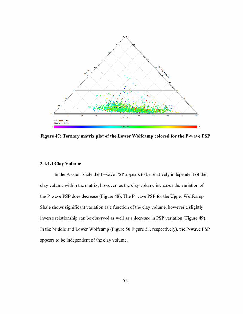
51
The Lower Wolfcamp has the highest concentration of clay of any of the
formations studied (Figure 47). On average the Lower Wolfcamp contains less than 10%
carbonate materials and 20-70% illite with the remaining being quartz. In the formation,
clay appears to be matrix supporting and there is not a distinct trend relating to the P-
wave PSP.
Figure 46: Ternary matrix plot of the Middle Wolfcamp colored for the
P-wave PSP
52
Figure 47: Ternary matrix plot of the Lower Wolfcamp colored for the P-wave PSP
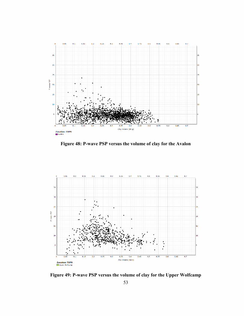
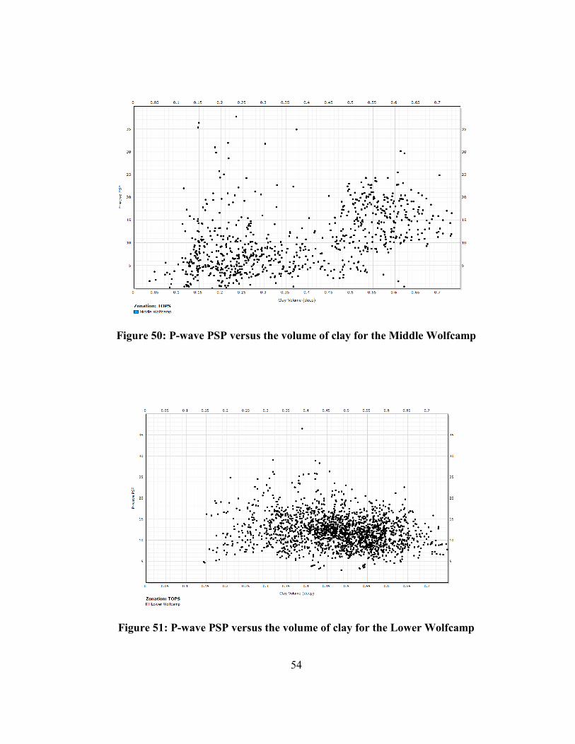
3.4.4.4 Clay Volume
In the Avalon Shale the P-wave PSP appears to be relatively independent of the
clay volume within the matrix; however, as the clay volume increases the variation of
the P-wave PSP does decrease (Figure 48). The P-wave PSP for the Upper Wolfcamp
Shale shows significant variation as a function of the clay volume, however a slightly
inverse relationship can be observed as well as a decrease in PSP variation (Figure 49).
In the Middle and Lower Wolfcamp (Figure 50 Figure 51, respectively), the P-wave PSP
appears to be independent of the clay volume.
53
Figure 48: P-wave PSP versus the volume of clay for the Avalon
Figure 49: P-wave PSP versus the volume of clay for the Upper Wolfcamp
54
Figure 50: P-wave PSP versus the volume of clay for the Middle Wolfcamp
Figure 51: P-wave PSP versus the volume of clay for the Lower Wolfcamp
55
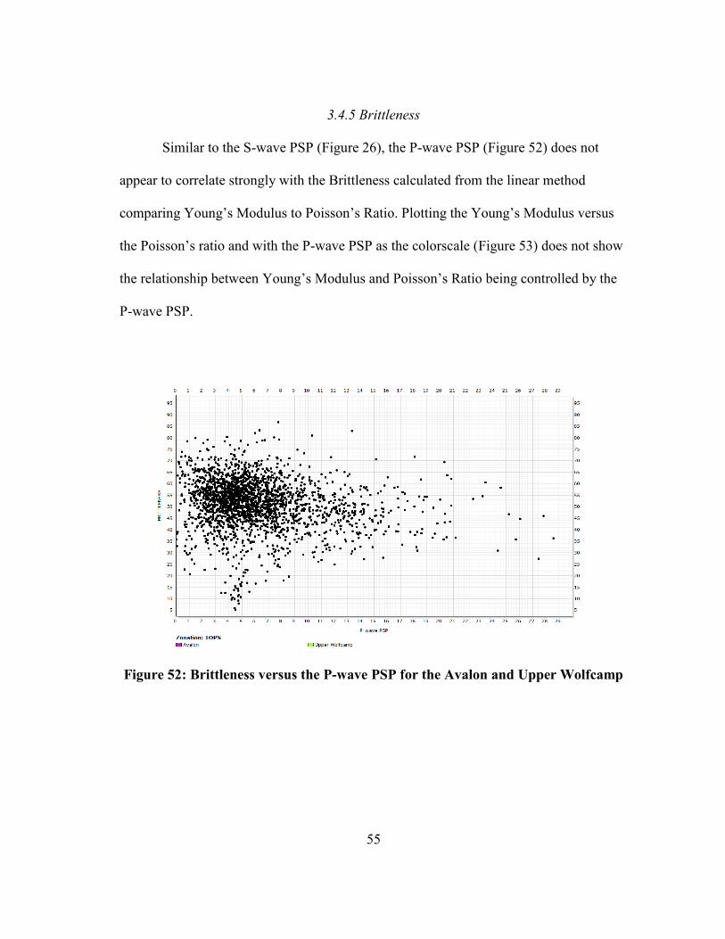
3.4.5 Brittleness
Similar to the S-wave PSP (Figure 26), the P-wave PSP (Figure 52) does not
appear to correlate strongly with the Brittleness calculated from the linear method
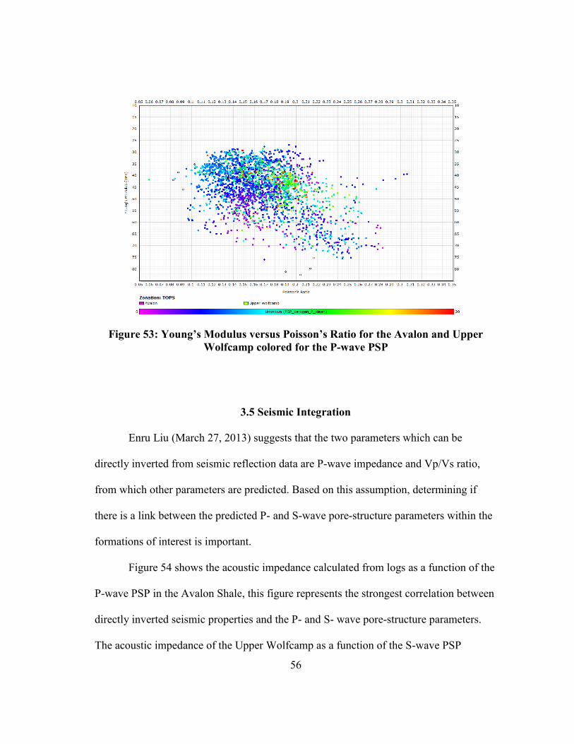
comparing Young’s Modulus to Poisson’s Ratio. Plotting the Young’s Modulus versus
the Poisson’s ratio and with the P-wave PSP as the colorscale (Figure 53) does not show
the relationship between Young’s Modulus and Poisson’s Ratio being controlled by the
P-wave PSP.
Figure 52: Brittleness versus the P-wave PSP for the Avalon and Upper Wolfcamp
56
Figure 53: Young’s Modulus versus Poisson’s Ratio for the Avalon and Upper
Wolfcamp colored for the P-wave PSP
3.5 Seismic Integration
Enru Liu (March 27, 2013) suggests that the two parameters which can be
directly inverted from seismic reflection data are P-wave impedance and Vp/Vs ratio,
from which other parameters are predicted. Based on this assumption, determining if
there is a link between the predicted P- and S-wave pore-structure parameters within the
formations of interest is important.
Figure 54 shows the acoustic impedance calculated from logs as a function of the
P-wave PSP in the Avalon Shale, this figure represents the strongest correlation between
directly inverted seismic properties and the P- and S- wave pore-structure parameters.
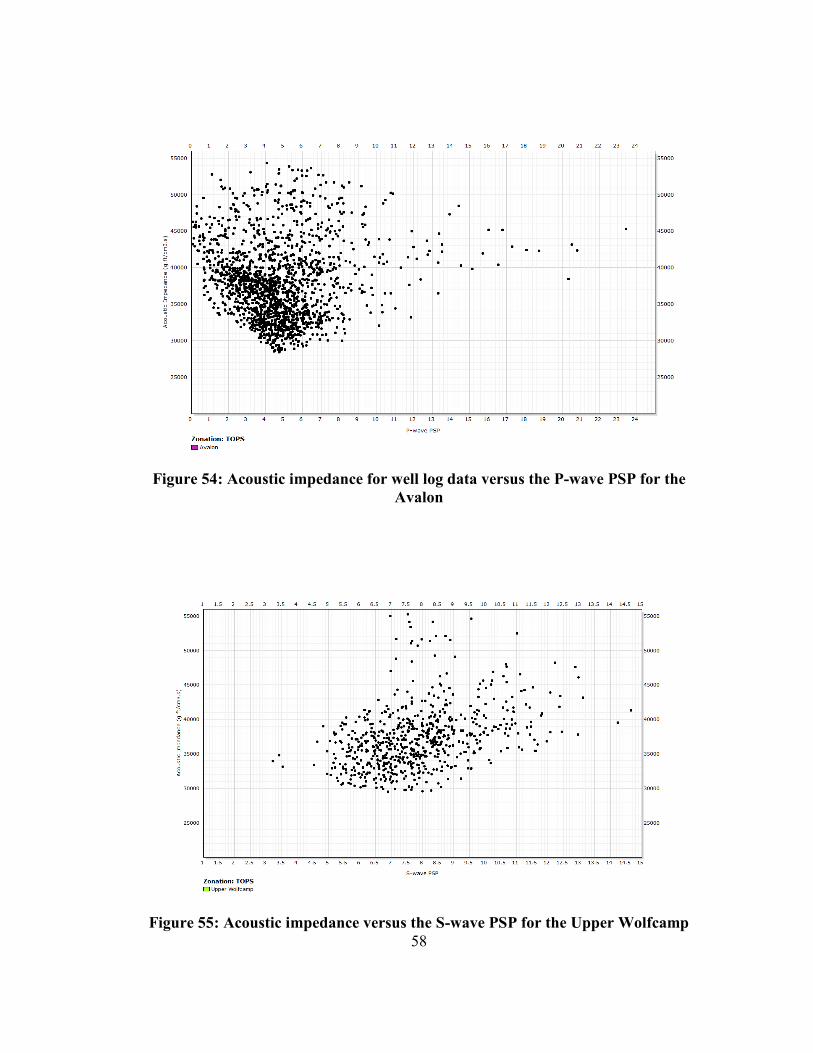
The acoustic impedance of the Upper Wolfcamp as a function of the S-wave PSP
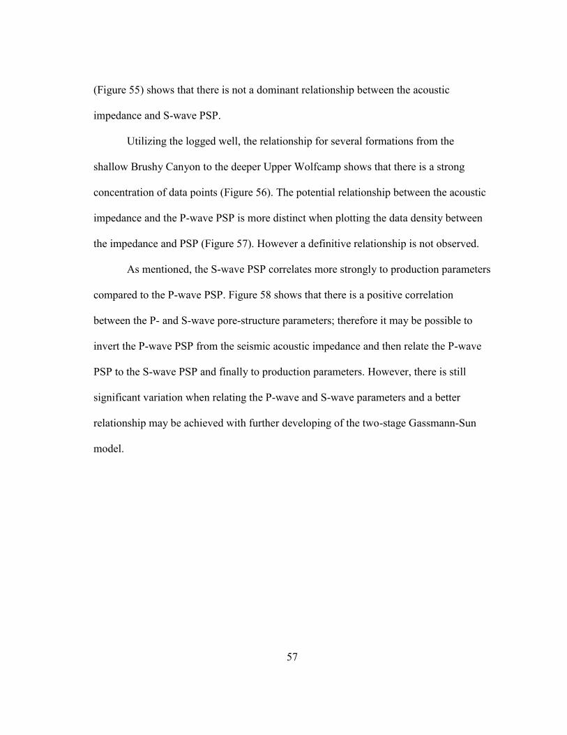
57
(Figure 55) shows that there is not a dominant relationship between the acoustic
impedance and S-wave PSP.
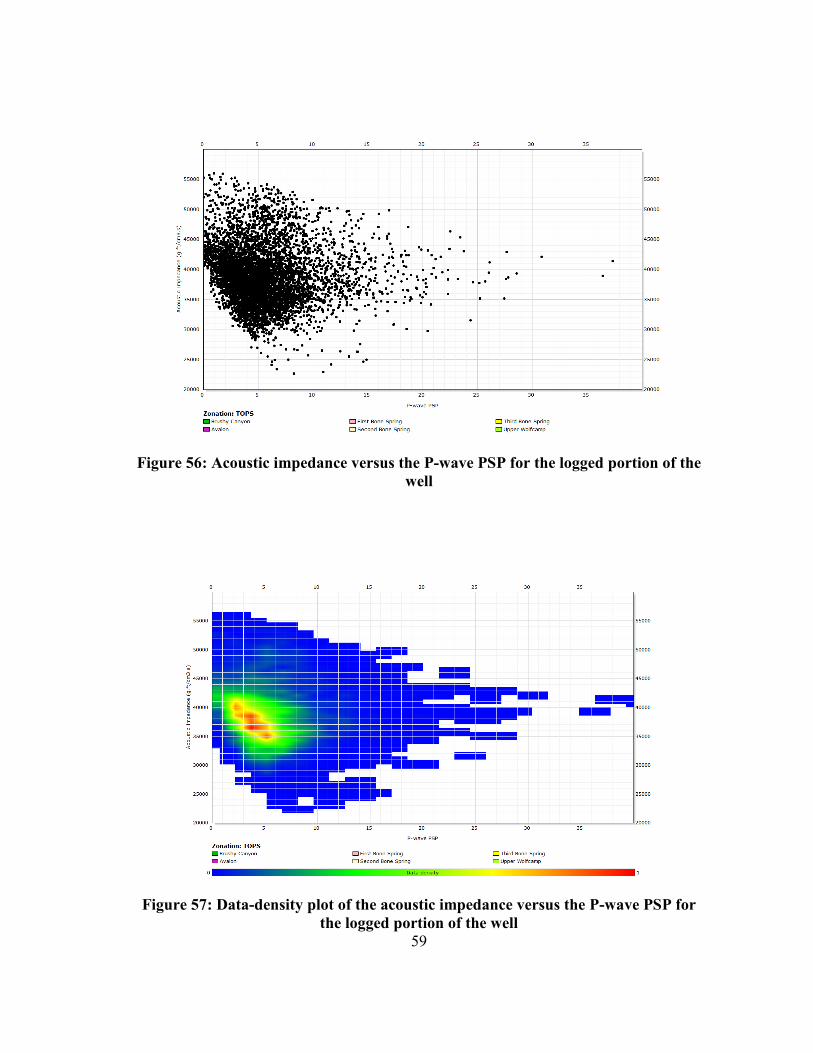
Utilizing the logged well, the relationship for several formations from the
shallow Brushy Canyon to the deeper Upper Wolfcamp shows that there is a strong
concentration of data points (Figure 56). The potential relationship between the acoustic
impedance and the P-wave PSP is more distinct when plotting the data density between
the impedance and PSP (Figure 57). However a definitive relationship is not observed.
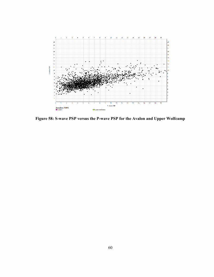
As mentioned, the S-wave PSP correlates more strongly to production parameters
compared to the P-wave PSP. Figure 58 shows that there is a positive correlation
between the P- and S-wave pore-structure parameters; therefore it may be possible to
invert the P-wave PSP from the seismic acoustic impedance and then relate the P-wave
PSP to the S-wave PSP and finally to production parameters. However, there is still
significant variation when relating the P-wave and S-wave parameters and a better
relationship may be achieved with further developing of the two-stage Gassmann-Sun
model.
58
Figure 54: Acoustic impedance for well log data versus the P-wave PSP for the
Avalon
Figure 55: Acoustic impedance versus the S-wave PSP for the Upper Wolfcamp
59
Figure 56: Acoustic impedance versus the P-wave PSP for the logged portion of the
well
Figure 57: Data-density plot of the acoustic impedance versus the P-wave PSP for
the logged portion of the well
60
Figure 58: S-wave PSP versus the P-wave PSP for the Avalon and Upper Wolfcamp
61
4. CONCLUSIONS
The bulk and shear moduli of an organic-rich shale formation is affected by
several factors that cause variations when other factors are held constant. This study
focused on those factors which are deemed crucial by industry for economical
production from organic-rich shale formations. The factors of interest are
lithology/mineralogy, TOC, kerogen volume, fluid saturation and thermal maturity. A
rock physics model that integrated Gassmann and Sun models in a two-stage rock
system was used to predict the P- and S-wave pore-structure parameters from the Sun
model to bridge the gap from well log properties to seismic measurements.
The S-wave PSP was found to correlate well with the shear modulus, decreasing
the shear modulus at a specific porosity for a constant porosity. Using data density, a
negative correlation of the S-wave PSP and hydrocarbon saturation was observed at
hydrocarbon saturations greater than 70%. A strong correlation between the S-wave PSP
and the weight percent of TOC was not observed, however it was observed that the
variation in the S-wave PSP decreases as both the TOC and hydrocarbon saturation
increase. When comparing the thermal maturity derived from pyrolysis the S-wave PSP
was observed to correlate positively as the maturity increased through the oil window
and into the condensate window. In the Avalon and Upper Wolfcamp Shales higher S-
wave PSP values correlated with higher concentrations of calcite/dolomite. The Middle
and Lower Wolfcamp contain the highest PSP values of the four formations of interest,
the higher PSP values correlated with higher concentrations of quartz. Figure 25
indicates a change in the relationship between the S-wave PSP and clay volume at
62
approximately 32%, similar to the critical clay volume described by Adesokan (2012).
The S-wave PSP was found to not correlate with the brittleness (Young’s Modulus and
Poisson’s Ratio) of the formation.
The P-wave PSP was found to correlate with the shear modulus, however the
correlation was weak in the Avalon Shale but slightly more apparent in the Upper,
Middle and Lower Wolfcamp. A similar correlation with hydrocarbon saturation was
observed above 70% saturation, however, the relationship was not nearly as strong as
with the S-wave PSP. The P-wave PSP was observed to decrease in variation with
increasing TOC and hydrocarbon saturation, however the P-wave PSP was still highly
varied at higher concentrations of organic matter. From pyrolysis the thermal maturity
appeared to have a positive correlation with the P-wave PSP, except the variation in the
P-wave PSP led to a weaker correlation than the S-wave PSP. In the ternary matrix
higher P-wave PSP often correlated with higher concentrations of calcite/dolomite. In
the Middle Wolfcamp higher PSP values were observed to correlate with clay volumes
greater than 50%. While in the Lower Wolfcamp there does not appear to be a definite
relationship between the P-wave PSP and the lithology. Comparing the clay volume and
P-wave PSP in the individual formations, a good correlation does not occur. Similar to
the S-wave PSP the P-wave PSP does not correlate with the brittleness of the formations.
In order to apply a rock physics model developed at the wellbore scale, a link to seismic
attributes must be identified. Investigating the formations individually, it was found that
the Avalon Shale showed the best correlation between the acoustic impedance and P-
wave PSP. However, it is necessary to potentially apply the rock physics model to the
63
entire well, therefore a data density plot of the data shows that the majority of the data
provides a correlation between acoustic impedance and the P-wave PSP. The S-wave
PSP was not found to correlate as well as the P-wave PSP even though the S-wave PSP
has shown to correlate better to rock properties of interest. A linear relationship is
observed between the P- and S-wave PSP’s which potentially allows the rock properties
to be linked through the P- and S-wave PSP’s to seismic attributes.
The ability to link rock properties to seismic attributes would allow for their
properties to be inverted from seismic attributes in an organic-rich shale formation.
These organic-rich shale formations rely on the amount of TOC, thermal maturation,
hydrocarbon saturation and clay volume to be economically produced. The potential
relationships presented show that through the use of the two-stage rock physics model
incorporating Gassmann and Sun models that the mentioned properties may be inverted
to further evaluate organic-rich shale formations as economic reservoirs. This research
on the most ideal case of organic-rich shale formations indicates how important the shear
wave may be to predicting petrophysical properties through rock physics models in
petroleum exploration.
64
REFERENCES
Adesokan, H., 2012. Rock Physics Based Determination of Reservoir Microstructure for
Reservoir Characterization. Ph.D., Texas A&M University, College Station, TX.
Alfred, D. and Vernik, L. 2012. A New Petrophysical Model for Organic Shales. Society
of Petrophysicists and Well Log Analysts Annual Meeting, Cartagena, Colombia.
Baker Hughes, 2004. Log Interpretation Charts, Baker Hughes, Houston, TX.
Gassmann, 1951. Elasticity of Porous Media. Vierteljahrsschrder Naturforschenden
Gesselschaft 96: 1-23.
Hashin, Z. and Shtrikman, S., 1962. A Variational Approach to the Theory of the Elastic
Behaviour of Polycrystals. Journal of the Mechanics and Physics of Solids, 10
(4): 343-352.
Jiang, M. and Spikes, K., 2011. Pore-Shape and Composition Effects on Rock-Physics
Modeling in the Haynesville Shale. SEG Annual Meeting, San Antonio, TX.
Krzikalla, F. 2010. Generalized Backus Theory for Poroelastic Solids. SEG Annual
Meeting, Denver, CO.
Lecompte, B. and Hursan, G., 2010. Quantifying Source Rock Maturity from Logs: How
to Get More Than Toc from Delta Log R. SPE Annual Technical Conference and
Exhibition, Florence, Italy.
Mavko, G., Mukerji, T., and Dvorkin, J., 2003. Rock Physics Handbook - Tools for
Seismic Analysis in Porous Media. Cambridge University Press, Cambridge, UK.
Mba, K. and Prasad, M., 2010. Mineralogy and Its Contribution to Anisotropy and
Kerogen Stiffness Variations with Maturity in the Bakken Shales. SEG Annual
Meeting, Denver, CO.
Rickman, R., Mullen, M.J., Petre, J.E. et al., 2008. A Practical Use of Shale
Petrophysics for Stimulation Design Optimization: All Shale Plays Are Not
Clones of the Barnett Shale. SPE Annual Technical Conference and Exhibition,
Denver, CO.
Sun, Y.F., 2000. Core-Log-Seismic Integration in Hemipelagic Marine Sediments on the
Eastern Flank of the Juan De Fuca Ridge. ODP Scientific Results 168: 21-35,
College Station, TX.
65
Sun, Y.F., 2004a. Pore Structure Effects on Elastic Wave Propagation in Rocks: Avo
Modelling. Journal of Geophysics Engineering 1 (268-276).
Sun, Y.F., 2004b. Sesimic Signatures of Rock Pore Structure. Applied Geophysics 1: 42-
49.
Vernik, L. and Kachanov, M., 2010. Modeling Elastic Properties of Siliciclastic Rocks.
GEOPHYSICS 75 (6): E171-E182.
Vernik, L. and Milovac, J., 2011. Rock Physics of Organic Shales. The Leading Edge 30
(3): 318-323.
Wang, Z. and Nur, A., 1992. Elastic Wave Velocities in Porous Media: A Theoretical
Recipe. Seismic and Acoustic Velocities in Reservoir Rocks, Society of
Exploration Geophysicists, 2: 1-35.
Ward, J., 2010. Kerogen Density in the Marcellus Shale. SPE Unconventional Gas
Conference, Pittsburgh, PA.
Wyllie, M.R., Gregory, A.R., and Gardner, L.W., 1956. Elastic Wave Velocities in
Heterogenous and Porous Media. GEOPHYSICS 21 (41-70).
Zhang, T., Dou, Q., Sun, Y. et al., 2012. Improving Porosity-Velocity Relations Using
Carbonate Pore Types. SEG Technical Program Expanded Abstracts 2012,
edition 1-5.
66
APPENDIX
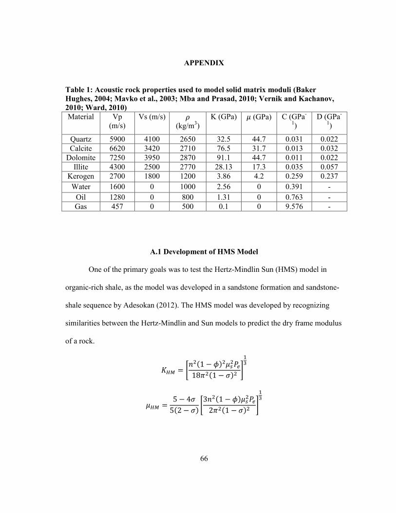
Table 1: Acoustic rock properties used to model solid matrix moduli (Baker
Hughes, 2004; Mavko et al., 2003; Mba and Prasad, 2010; Vernik and Kachanov,
2010; Ward, 2010)
Material Vp
(m/s)
Vs (m/s) (kg/m
3)
K (GPa) (GPa) C (GPa-
1)
D (GPa-
1)
Quartz 5900 4100 2650 32.5 44.7 0.031 0.022
Calcite 6620 3420 2710 76.5 31.7 0.013 0.032
Dolomite 7250 3950 2870 91.1 44.7 0.011 0.022
Illite 4300 2500 2770 28.13 17.3 0.035 0.057
Kerogen 2700 1800 1200 3.86 4.2 0.259 0.237
Water 1600 0 1000 2.56 0 0.391 -
Oil 1280 0 800 1.31 0 0.763 -
Gas 457 0 500 0.1 0 9.576 -
A.1 Development of HMS Model
One of the primary goals was to test the Hertz-Mindlin Sun (HMS) model in
organic-rich shale, as the model was developed in a sandstone formation and sandstone-
shale sequence by Adesokan (2012). The HMS model was developed by recognizing
similarities between the Hertz-Mindlin and Sun models to predict the dry frame modulus
of a rock.
[ ( )
( )
]
( )[ ( )
( )
]
67
Where is the coordination number, defined as the average number of contacts
between grains in the volume and is the effective pressure acting on the formation as a
function of overburden pressure and pore pressure.
∫ ( )
Using Gassmann’s equation, the Hertz-Mindlin model originally over-predicted
the measured velocity by 2% in intervals with clay volumes less than 25%. However in
formations with clay volume greater than 25% the Hertz-Mindlin model over-predicted
the velocity by 69%. Adesokan recognized the similarities between the models and
inserted the Sun model into the Hertz-Mindlin model:
[ ( )
( )
]
( )[ ( )
( )
]
Using the previous methodology, Adesokan showed that the new Hertz-Mindlin
Sun model over-predicted the measured velocity by 1.8% in formations with less than
25% clay volume. More importantly the new model over-predicted the measured
velocity by 4% in formation with greater than 25% clay volume greatly enhancing the
velocity prediction by incorporating the pore-structure parameter. This showed that it is
important to account for the different pore aspect ratio of shaly grains when they occur
in formations with greater than 25% clay volume.
68
A.1.1 Testing of HMS Model
Using log measurements and a five-component matrix model, Gassmann and Sun
models were used to predict the P- and S-wave PSP. The HMS model along with the
predicted PSP was then used to predict the dry bulk and shear moduli. Once the dry
moduli were predicted using the HMS model, Gassmann was used to predict the
saturated moduli. From the saturated moduli the compressional velocity was predicted
(Figure 59). The reconstructed compressional velocity shows that it does not correlate
with the measured log velocity and that there is significant error from the model;
therefore the conclusion that the HMS model is not accurate in organic-rich shales can
be made.
Figure 59: Reconstructed compressional velocity versus log measured
compressional velocity along with 1:1 line