ROBUSTNESS OF TWO-PHASE REGRESSION TESTS

REVSTAT – Statistical Journal

Volume 3, Number 1, June 2005, 1–18

ROBUSTNESS OF TWO-PHASE REGRESSION

TESTS

Authors: Carlos A.R. Diniz

– Departamento de Estatıstica, Universidade Federal de Sao Carlos,Sao Paulo, Brazil ([email protected])

Luis Corte Brochi

– Departamento de Estatıstica, Universidade Federal de Sao Carlos,Sao Paulo Brazil ([email protected])

Received: February 2003 Revised: July 2004 Accepted: December 2004

Abstract:

• This article studies the robustness of different likelihood ratio tests proposed byQuandt ([1]) and ([2]), (Q-Test), Kim and Siegmund ([3]), (KS-Test), and Kim ([4]),(K-Test), to detect a change in simple linear regression models. These tests are eval-uated and compared with respect to their performance taking into account differentscenarios, such as, different error distributions, different sample sizes, different loca-tions of the change point and departure from the homoscedasticity. Two differentalternatives are considered: i) with a change in the intercept from one model to theother with the same slope and ii) with a change in both the intercept and slope.

The simulation results reveal that the KS-Test is superior to the Q-Test for bothmodels considered while the K-Test is more powerful than the other two tests fornonhomogeneous models with a known variance.

Key-Words:

• segmented regression models; likelihood ratio tests; robustness.

AMS Subject Classification:

• 62J02, 62F03.

2 Diniz and Brochi

Robustness of two-phase regression tests 3

1. INTRODUCTION

The use of models involving a sequence of submodels has been widely ap-

plied in areas such as economics, medicine and biology, among others. These

types of models, denoted by segmented (or switching or multi-phase) regression

models, are useful when it is believed that the model parameters change after an

unknown time or in some region of the domain of the predictor variables.

A simple segmented regression model, in the case that a sequence of obser-

vations (xi, yi), i=1, 2, ..., n, is considered, can be written in the following way

yi =

{α1 + β1xi + εi, if xi 6 r

α2 + β2 xi + εi, if xi > r ,(1.1)

where α1, α2, β1, β2 and r are unknown parameters and the errors εi have distri-

bution N(0, σ2). The submodels in (1.1) are referred to as regimes or segments

and the point r as the change point.

Segmented regression models are divided into two types. One where the

model is assumed to be continuous at the change point, and the other where

it is not. The inferential theory is completely different for each type of model

(Hawkins ([5])). The emphasis in this article is on the discontinuous model.

The linear-linear segmented regression model proposed by Quandt ([1]) is

similar to model (1.1), except that the change point is identified by the observa-

tion order instead of the observation value as above. Moreover, the model (1.1)

assumes homoscedasticity while the Quandt model assumes heteroscedasticity.

Considering a sequence of observations (xi, yi), i = 1, 2, ..., n, the Quandt

two-phase regression model is given by

yi =

{α1 + β1xi + εi, if i = 1, ..., k

α2 + β2 xi + εi, if i = k+1, ..., n ,(1.2)

where the εi have independent normal distributions with mean zero and variance

σ21 if i6 k and variance σ2

2 if i>k. The parameters α1, α2, β1, β2 and k are all

unknown.

Various tests for the presence of a change point based on the likelihood

ratio are discussed in the statistics literature. Quandt ([1], [2]) was the first

to propose a likelihood ratio test to detect the presence of a change point in

a simple linear regression model. Hinkley ([6]) derived the asymptotic distri-

bution of the maximum likelihood estimate of a change point and the asymp-

totic distribution of the likelihood ratio statistics for testing hypotheses of no

4 Diniz and Brochi

change in (1.2), where the independent observations x1, ..., xn, are ordered, the

change point k is unknown and the errors εi are considered uncorrelated N(0, σ2).

Furthermore, it is assumed that xk6γ6xk+1, where γ = (α1− α2)/(β2 − β1)

is the intersection of the two regression lines. Hinkley ([7]) discussed infer-

ence concerning a change point considering the hypothesis H0 : k = k0 versus the

one-sided alternative H1 : k > k0 or versus the two-sided alternative H2 : k 6= k0.

Brown et al. ([8]) described tests for detecting departures from constancy of re-

gression relationships over time and illustrated the application of these tests with

three sets of real data. Maronna and Yohai ([9]) derived the likelihood ratio test

for the hypothesis that a systematic change has occurred after some point in the

intercept alone. Worsley ([10]) found exact and approximate bounds for the null

distributions of likelihood ratio statistics for testing hypotheses of no change in

the two-phase multiple regression model

yi =

{x

′

i β + εi, if i = 1, ..., k

x′

i β∗ + εi, if i = k+1, ..., n ,

(1.3)

where p 6 k 6 n−p, xi is a p-component vector of independent variables and β

and β∗ are p-component vectors of unknown parameters. His numerical results

indicated that the accuracy of the approximation of the upper bound is very

good for small samples. Kim and Siegmund ([3]) consider likelihood ratio tests

for change point problems in simple linear regression models. They also present

a review on segmented regression models and some real problems that motivated

research in this area. Some of these problems are examined using change point

methods by Worsley ([11]) and Raferty and Akman ([12]). Kim ([4]) derived

the likelihood ratio tests for a change in simple linear regression with unequal

variances. Kim and Cai ([13]) examined the distributional robustness of the like-

lihood ratio tests discussed by Kim and Sigmund ([3]) in a simple linear regression.

They showed that these statistics converge to the same limiting distributions re-

gardless of the underlying distribution. Through simulation the observed distri-

butional insensitivity of the test statistics is observed when the errors follow a

lognormal, a Weibull, or a contaminated normal distribution. Kim ([4]), using

some numerical examples, examined the robustness to heteroscedasticity of these

tests.

In this paper different likelihood ratio tests (Quandt ([1]) and ([2]), Kim and

Siegmund ([3]) and Kim ([4])) to detect a change on a simple linear regression,

are presented. The tests are evaluated and compared regarding their perfor-

mance in different scenarios. Our main concern is to assist the user of such tests

to decide which test is preferable to use and under which circumstances. The

article is organized as follows. In Section 2, the likelihood ratio tests proposed by

Quandt ([1]) and ([2]), Kim and Siegmund ([3]) and Kim ([4]) will be described.

In Section 3, via Monte Carlo simulations, the performance of the tests discussed

in Section 2 will be assessed and compared. Final comments on the results,

presented in Section 4, will conclude the paper.


2. TEST STATISTICS

In this Section the likelihood ratio tests proposed by Quandt ([1]) and ([2]),

Kim and Siegmund ([3]) and Kim ([4]) are described in more detail. In all the

cases the model (1.2) is considered.

2.1. Likelihood Ratio Test by Quandt (Q-Test)

The test described by Quandt ([1]) and ([2]) is used for testing the hy-

pothesis that no change has occurred against the alternative that a change took

place. That is, H0 : α1= α2, β1= β2, σ1= σ2 against H1 : α1 6= α2 or β1 6= β2 or

σ1 6= σ2. The error terms εi are independently and normally distributed N(0, σ21)

for i = 1, ..., k and N(0, σ22) for i = k+1, ..., n.

The likelihood ratio λ is defined as

λ =l(k)

l(n),

where l(n) is the maximum of the likelihood function over only a single phase

and l(k) is the maximum of the likelihood function over the presence of a change

point. That is,

λ =exp

[− log(2π)

n2 − log σn − n

2

]

exp[− log(2π)

n2 − log σk1 − log σn−k2 − n

2

]

=σk1 σ

n−k2

σn,

where σ1 and σ2 are the estimates of the standard errors of the two regression

lines, σ is the estimate of the standard error of the overall regression based on all

observations and the constant k is chosen in order to minimize λ. On the basis

of empirical distributions resulting from sampling experiments, Quandt ([1]) con-

cluded that the distribution of −2 log λ can not be assumed to be χ2 distribution

with 4 degrees of freedom.

2.2. Likelihood Ratio Tests by Kim and Siegmund (KS-Test)

Kim and Siegmund ([3]), assuming the model (1.2) with homoscedasticity,

consider tests of the following hypotheses:

6 Diniz and Brochi

H0 : β1= β2 and α1= α2 against the alternatives

(i) H1 : β1= β2 and there exists a k (16k<n) such that α1 6= α2 or

(ii) H2 : there exists a k (16k<n) such that β1 6= β2 and α1 6= α2.

The alternative (i) specifies that a change has occurred after some point in

the intercept alone and alternative (ii) specifies that a change has occurred after

some point in both intercept and slope.

The likelihood ratio test of H0 against H1 rejects H0 for large values of

maxn06i6n1

|Un(i)| /σ ,

where nj= ntj , j=0, 1, for 0<t0<t1<1, and

Un(i) = (αi − α∗i )

(i (1− i/n)

1 − i(xi − xn)2/{Qxxn(1 − i/n)

})1/2

.

The likelihood ratio test of H0 against H2 rejects H0 for large values of

σ−2 maxn06i6n1

{n i (yi − yn)

2

n− i+Q2xyi

Qxxi+Q∗2xyi

Q∗xxi

−Q2xyn

Qxxn

},

where, following Kim and Siegmund ([3]) notation,

xi = i−1

i∑

k=1

xk , yi = i−1

i∑

k=1

yk , αi = yi − β xi , α∗i = y∗i − β x∗i ,

x∗i = (n−i)−1

n∑

k=i+1

xk , y∗i = (n−i)−1

n∑

k=i+1

yk , Qxyi =i∑

k=1

(xk− xi) (yk− yi) ,

Qxxi =i∑

k=1

(xk− xi)2 , Q∗

xxi =n∑

k=i+1

(xk− x∗i )2 , ... ,

Qxxn =n∑

k=1

(xk− xn)2 , Qxyn =

n∑

k=1

(xk− xn) (yk− yn) ,

β = Qxyn/Qxxn and σ2 = n−1(Qyyn −Q2

xyn/Qxxn

).

In these tests and in the tests by Kim, the values for t0 and t1 depend on

the feeling we have concerning the location of the change point. This impression

comes from a scatterplot of y and x. In this study we will use t0= 0.1 and t1= 0.9.


2.3. Likelihood Ratio Tests by Kim (K-Test)

Kim ([4]) studied likelihood ratio tests for a change in a simple linear re-

gression model considering the two types of alternatives presented in the previous

subsection. It is assumed that the error variance is non-homogeneous, that is, the

error terms follow N(0, σ2i ), where σ

2i =σ

2/wi and the wi’s are positive constants.

The likelihood ratio statistics is denoted by weighted likelihood ratio statistics.

The weighted likelihood ratio statistics to test H0 against H1, (WLRS1),

is given by

σ−1 maxn06i6n1

|Uw,n(i)|(2.1)

where

Uw,n(i) =

i∑k=1

wkn∑k=1

wk

n∑k=i+1

wk

1

2

yw,i − yw,n − βw · (xw,i − xw,n)[1−{

i∑k=1

wkn∑k=1

wk/ n∑k=i+1

wk

}(xw,i− xw,n)

2/Qxxn

]1

2

.

The weighted likelihood ratio statistics to test H0 against H2, (WLRS2), is given

by

σ−2 maxn06i6n1

|Vw,n(i)| ,(2.2)

where

Vw,n(i) =

i∑k=1

wkn∑k=1

wk

n∑k=i+1

wk

(yw,i − yw,n)2 +

Q2xyi

Qxxi+Q∗2xyi

Q∗xxi

−Q2xyn

Qxxn.

In both tests nj= ntj , j=0, 1, for 0 < t0 < t1 < 1, and following Kim ([4])

notation,

xw,i =

(i∑

k=1

wk

)−1 i∑

k=1

wk xk , x∗w,i =

(n∑

k=i+1

wk

)−1 n∑

k=i+1

wk xk ,

yw,i =

(i∑

k=1

wk

)−1 i∑

k=1

wk yk , y∗w,i =

(n∑

k=i+1

wk

)−1 n∑

k=i+1

wk yk ,

8 Diniz and Brochi

Qxxi =i∑

k=1

wk (xk− xw,i)2 , Q∗

xxi =n∑

k=i+1

wk(xk− x∗w,i

)2,

Qyyi =i∑

k=1

wk (yk− yw,i)2 , Q∗

yyi =n∑

k=i+1

wk(yk− y∗w,i

)2,

Qxyi =i∑

k=1

wk (xk− xw,i) (yk− yw,i) ,

Qxxn =n∑

k=1

wk (xk− xw,n)2 , Qxyn =

n∑

k=1

wk (xk− xw,n) (yk− yw,n) ,

βw = Qxyn/Qxxn and σ2 = n−1(Qyyn −Q2

xyn/Qxxn

).

Kim ([4]) also presents approximations of the p-values of the WLRS (2.1)

and (2.2).

3. PERFORMANCE OF THE TESTS

To assess and compare the performance of the tests described in the pre-

vious section we carried out a Monte Carlo simulation taking into account dif-

ferent scenarios, such as, different error distributions, different sample sizes, dif-

ferent locations of the change point and departure from the homoscedasticity as-

sumption. In all the cases two different alternative hypotheses were considered:

i) with a change in the intercept from one model to the other with the same slope,

and ii) with a change in both intercept and slope.

In the simulation process, for each model, the sequence of observations

(x1, y1) , ..., (xn, yn), where xi= i/n, i=1, ..., n and yi satisfying the model (1.2),

were generated 5,000 times. To calculate the distributional insensitivity of the

tests the following distributions for the errors were considered: N(0, 1), N(0, 1)

for one regime and N(0, 4) for the other, normal with variance given by 1/wi,

where wi = (1 + i/n)2, contaminated normal using the mixture distribution

0.95N(0, 1) + 0.5N(0, 9), exponential(1), Weibull(α,γ), with α = 1.5 and γ =

1/(21/2α{Γ(2/α + 1) − Γ2(1/α + 1)}0.5), and lognormal(α, γ), with α=0.1 and

γ = {exp(2α) − exp(α)}−0.5. For more details for the choice of these parameters

interested readers can see Kim and Cai (1993).


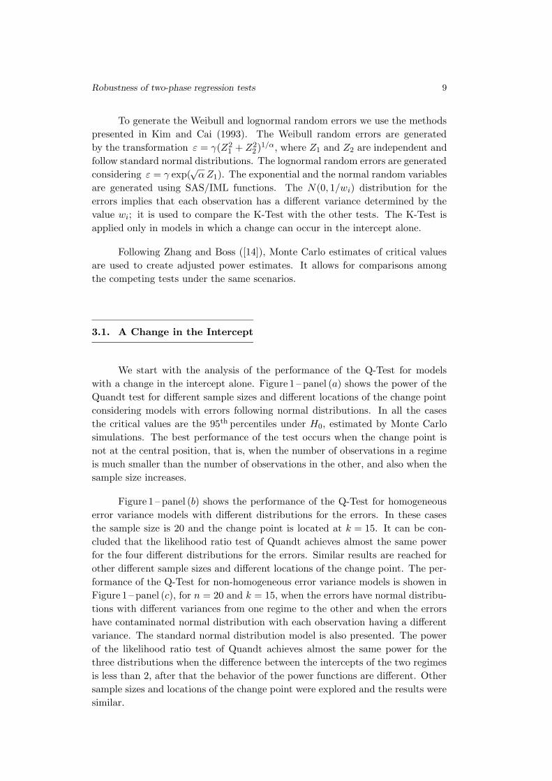
To generate the Weibull and lognormal random errors we use the methods

presented in Kim and Cai (1993). The Weibull random errors are generated

by the transformation ε = γ(Z21 + Z2

2 )1/α, where Z1 and Z2 are independent and

follow standard normal distributions. The lognormal random errors are generated

considering ε = γ exp(√αZ1). The exponential and the normal random variables

are generated using SAS/IML functions. The N(0, 1/wi) distribution for the

errors implies that each observation has a different variance determined by the

value wi; it is used to compare the K-Test with the other tests. The K-Test is

applied only in models in which a change can occur in the intercept alone.

Following Zhang and Boss ([14]), Monte Carlo estimates of critical values

are used to create adjusted power estimates. It allows for comparisons among

the competing tests under the same scenarios.

3.1. A Change in the Intercept

We start with the analysis of the performance of the Q-Test for models

with a change in the intercept alone. Figure 1 – panel (a) shows the power of the

Quandt test for different sample sizes and different locations of the change point

considering models with errors following normal distributions. In all the cases

the critical values are the 95th percentiles under H0, estimated by Monte Carlo

simulations. The best performance of the test occurs when the change point is

not at the central position, that is, when the number of observations in a regime

is much smaller than the number of observations in the other, and also when the

sample size increases.

Figure 1 – panel (b) shows the performance of the Q-Test for homogeneous

error variance models with different distributions for the errors. In these cases

the sample size is 20 and the change point is located at k = 15. It can be con-

cluded that the likelihood ratio test of Quandt achieves almost the same power

for the four different distributions for the errors. Similar results are reached for

other different sample sizes and different locations of the change point. The per-

formance of the Q-Test for non-homogeneous error variance models is showen in

Figure 1 – panel (c), for n = 20 and k = 15, when the errors have normal distribu-

tions with different variances from one regime to the other and when the errors

have contaminated normal distribution with each observation having a different

variance. The standard normal distribution model is also presented. The power

of the likelihood ratio test of Quandt achieves almost the same power for the

three distributions when the difference between the intercepts of the two regimes

is less than 2, after that the behavior of the power functions are different. Other

sample sizes and locations of the change point were explored and the results were

similar.

10 Diniz and Brochi

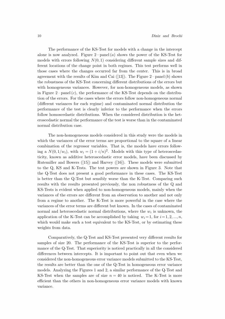
The performance of the KS-Test for models with a change in the intercept

alone is now analyzed. Figure 2 – panel (a) shows the power of the KS-Test for

models with errors following N(0, 1) considering different sample sizes and dif-

ferent locations of the change point in both regimes. This test performs well in

those cases where the changes occurred far from the center. This is in broad

agreement with the results of Kim and Cai ([13]). The Figure 2 – panel (b) shows

the robustness of the KS-Test concerning different distributions of the errors but

with homogeneous variances. However, for non-homogeneous models, as shown

in Figure 2 – panel (c), the performance of the KS-Test depends on the distribu-

tion of the errors. For the cases where the errors follow non-homogeneous normal

(different variances for each regime) and contaminated normal distribution the

performance of the test is clearly inferior to the performance when the errors

follow homoscedastic distributions. When the considered distribution is the het-

eroscedastic normal the performance of the test is worse than in the contaminated

normal distribution case.

The non-homogeneous models considered in this study were the models in

which the variances of the error terms are proportional to the square of a linear

combination of the regressor variables. That is, the models have errors follow-

ing a N(0, 1/wi), with wi = (1 + i/n)2. Models with this type of heteroscedas-

ticity, known as additive heteroscedastic error models, have been discussed by

Rutemiller and Bowers ([15]) and Harvey ([16]). These models were submitted

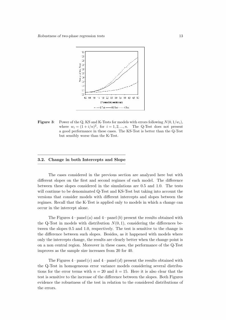
to the Q, KS and K-Tests. The test powers are shown in Figure 3. Note that

the Q-Test does not present a good performance in these cases. The KS-Test

is better than the Q-Test but sensibly worse than the K-Test. Comparing such

results with the results presented previously, the non robustness of the Q and

KS-Tests is evident when applied to non-homogeneous models, mainly when the

variances of the errors are different from an observation to another and not only

from a regime to another. The K-Test is more powerful in the case where the

variances of the error terms are different but known. In the cases of contaminated

normal and heteroscedastic normal distributions, where the wi is unknown, the

application of the K-Test can be accomplished by taking wi=1, for i=1, 2, ..., n,

which would make such a test equivalent to the KS-Test, or by estimating these

weights from data.

Comparatively, the Q-Test and KS-Test presented very different results for

samples of size 20. The performance of the KS-Test is superior to the perfor-

mance of the Q-Test. That superiority is noticed practically in all the considered

differences between intercepts. It is important to point out that even when we

considered the non-homogeneous error variance models submitted to the KS-Test,

the results are better than the one of the Q-Test in homogeneous error variance

models. Analyzing the Figures 1 and 2, a similar performance of the Q-Test and

KS-Test when the samples are of size n = 40 is noticed. The K-Test is more

efficient than the others in non-homogeneous error variance models with known

variance.


(a) (b)

(c)

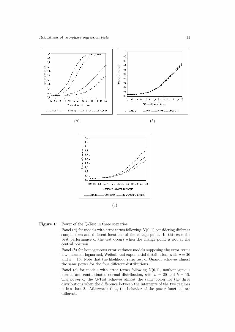
Figure 1: Power of the Q-Test in three scenarios:

Panel (a) for models with error terms following N(0, 1) considering differentsample sizes and different locations of the change point. In this case thebest performance of the test occurs when the change point is not at thecentral position.

Panel (b) for homogeneous error variance models supposing the error termshave normal, lognormal, Weibull and exponential distribution, with n = 20and k = 15. Note that the likelihood ratio test of Quandt achieves almostthe same power for the four different distributions.

Panel (c) for models with error terms following N(0,1), nonhomogenousnormal and contaminated normal distribution, with n = 20 and k = 15.The power of the Q-Test achieves almost the same power for the threedistributions when the difference between the intercepts of the two regimesis less than 2. Afterwards that, the behavior of the power functions aredifferent.

12 Diniz and Brochi

(a) (b)

(c)

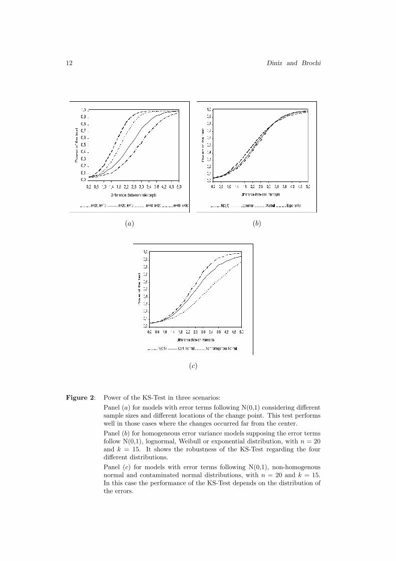
Figure 2: Power of the KS-Test in three scenarios:

Panel (a) for models with error terms following N(0,1) considering differentsample sizes and different locations of the change point. This test performswell in those cases where the changes occurred far from the center.

Panel (b) for homogeneous error variance models supposing the error termsfollow N(0,1), lognormal, Weibull or exponential distribution, with n = 20and k = 15. It shows the robustness of the KS-Test regarding the fourdifferent distributions.

Panel (c) for models with error terms following N(0,1), non-homogenousnormal and contaminated normal distributions, with n = 20 and k = 15.In this case the performance of the KS-Test depends on the distribution ofthe errors.


Figure 3: Power of the Q, KS and K-Tests for models with errors following N(0, 1/wi),where wi = (1 + i/n)2, for i = 1, 2, ..., n. The Q-Test does not presenta good performance in these cases. The KS-Test is better than the Q-Testbut sensibly worse than the K-Test.

3.2. Change in both Intercepts and Slope

The cases considered in the previous section are analyzed here but with

different slopes on the first and second regimes of each model. The difference

between these slopes considered in the simulations are 0.5 and 1.0. The tests

will continue to be denominated Q-Test and KS-Test but taking into account the

versions that consider models with different intercepts and slopes between the

regimes. Recall that the K-Test is applied only to models in which a change can

occur in the intercept alone.

The Figures 4 – panel (a) and 4 – panel (b) present the results obtained with

the Q-Test in models with distribution N(0, 1), considering the differences be-

tween the slopes 0.5 and 1.0, respectively. The test is sensitive to the change in

the difference between such slopes. Besides, as it happened with models where

only the intercepts change, the results are clearly better when the change point is

on a non central region. Moreover in these cases, the performance of the Q-Test

improves as the sample size increases from 20 for 40.

The Figures 4 – panel (c) and 4 – panel (d) present the results obtained with

the Q-Test in homogeneous error variance models considering several distribu-

tions for the error terms with n = 20 and k = 15. Here it is also clear that the

test is sensitive to the increase of the difference between the slopes. Both Figures

evidence the robustness of the test in relation to the considered distributions of

the errors.

14 Diniz and Brochi

(a) (b)

(c) (d)

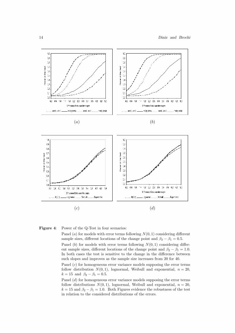
Figure 4: Power of the Q-Test in four scenarios:

Panel (a) for models with error terms following N(0, 1) considering differentsample sizes, different locations of the change point and β2 − β1 = 0.5.

Panel (b) for models with error terms following N(0, 1) considering differ-ent sample sizes, different locations of the change point and β2 − β1 = 1.0.In both cases the test is sensitive to the change in the difference betweensuch slopes and improves as the sample size increases from 20 for 40.

Panel (c) for homogeneous error variance models supposing the error termsfollow distribution N(0, 1), lognormal, Weibull and exponential, n = 20,k = 15 and β2 − β1 = 0.5.

Panel (d) for homogeneous error variance models supposing the error termsfollow distributions N(0, 1), lognormal, Weibull and exponential, n = 20,k = 15 and β2 −β1 = 1.0. Both Figures evidence the robustness of the testin relation to the considered distributions of the errors.


The performance of the Q-Test in non-homogeneous error variance models

in comparison to the case N(0, 1) can be seen in Figures 5 – panel (a) and

5 – panel (b), these also evidence that the test is sensitive to the increase of the

difference between the slopes. Once again, the non robustness of the test studied

in relation to the presence of heteroscedasticity can be clearly seen.

(a) (b)

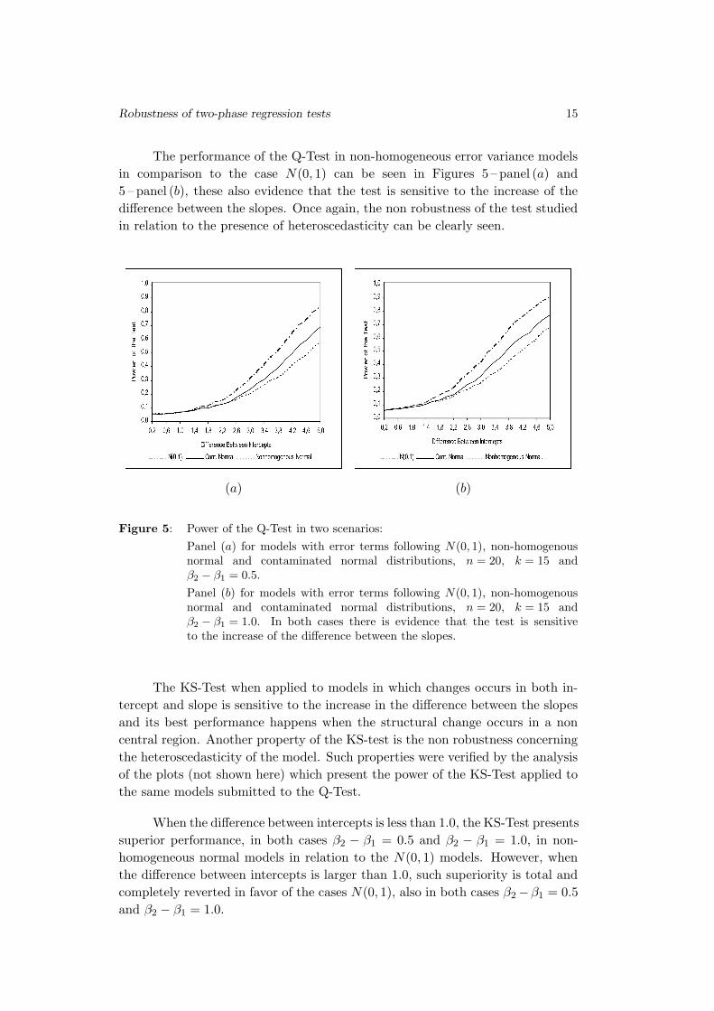
Figure 5: Power of the Q-Test in two scenarios:

Panel (a) for models with error terms following N(0, 1), non-homogenousnormal and contaminated normal distributions, n = 20, k = 15 andβ2 − β1 = 0.5.

Panel (b) for models with error terms following N(0, 1), non-homogenousnormal and contaminated normal distributions, n = 20, k = 15 andβ2 − β1 = 1.0. In both cases there is evidence that the test is sensitiveto the increase of the difference between the slopes.

The KS-Test when applied to models in which changes occurs in both in-

tercept and slope is sensitive to the increase in the difference between the slopes

and its best performance happens when the structural change occurs in a non

central region. Another property of the KS-test is the non robustness concerning

the heteroscedasticity of the model. Such properties were verified by the analysis

of the plots (not shown here) which present the power of the KS-Test applied to

the same models submitted to the Q-Test.

When the difference between intercepts is less than 1.0, the KS-Test presents

superior performance, in both cases β2 − β1 = 0.5 and β2 − β1 = 1.0, in non-

homogeneous normal models in relation to the N(0, 1) models. However, when

the difference between intercepts is larger than 1.0, such superiority is total and

completely reverted in favor of the cases N(0, 1), also in both cases β2 −β1 = 0.5

and β2 − β1 = 1.0.

16 Diniz and Brochi

Q-Test and KS-Test are sensitive to the alterations of differences between

intercepts and differences between slopes, besides both tests present better per-

formances when the structural change happens in a non central region. Another

characteristic of the Q-Test and KS-Test is the non robustness of their perfor-

mance in non-homogeneous error variance models in relation to the homogeneous

models.

In all the presented cases the KS-Test performs better than the Q-Test.

Both are shown to be robust regarding the different distributions considered in

homogeneous models, except the KS-Test when applied in models with error

following exponential distribution. However, even presenting inferior power in

the exponential case, the KS-Test has more power than the Q-Test in all the

homogeneous cases.

4. WORKING WITH OUTLIERS

In this section a small investigation of the sensitivity of the tests referring

to outlying observations is presented. New data sets, contaminated with outliers,

are simulated from the model (1.2) and the power results for the three tests,

for some scenarios, are explored. This investigation involves the power of the

Q-test, KS-Test and K-test considering data sets with and without outliers, dif-

ferent sample sizes and different locations of the change point, for errors following

normal distributions. In all the cases the critical values are the 95th percentiles

under H0, estimated by Monte Carlo simulations.

(a) (b)

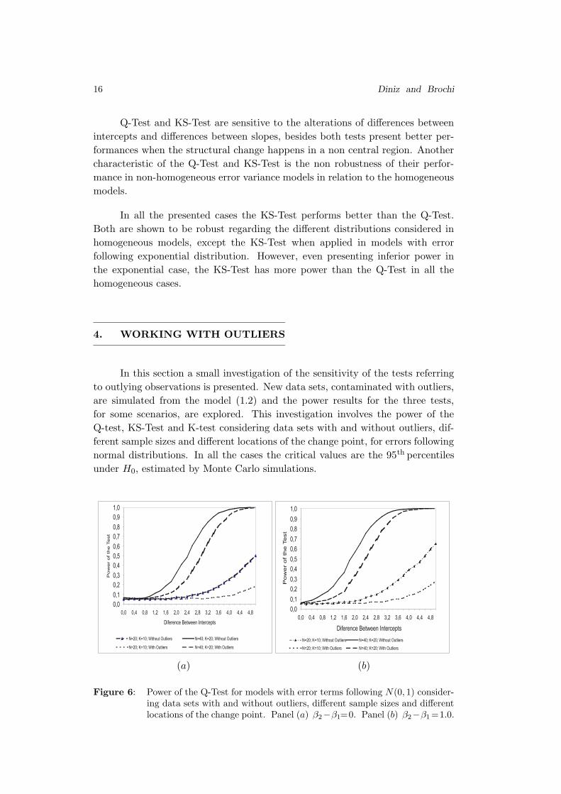
Figure 6: Power of the Q-Test for models with error terms following N(0, 1) consider-ing data sets with and without outliers, different sample sizes and differentlocations of the change point. Panel (a) β2−β1=0. Panel (b) β2−β1=1.0.


For the Q-Test and KS-Test, if the outliers are clearly present in one of

the regimes, inspection of the results reveals that the cases without outliers have

slightly more power when compared to the cases with outliers, but for the K-test

the power of cases with and without outliers are comparable.

For the three studied tests, the cases where the outliers are clearly in the

change point region are slightly more powerful than those cases without outliers.

The reason for that can reside in the fact that the simulated outliers reinforced

the presence of change points.

5. CONCLUDING REMARKS

The robustness of different likelihood ratio tests was investigated under

different scenarios via a simulation study as presented in Section 3. With the

exception of the study by Kim and Cai ([13]) there has been little work done

for a comprehensive discussion of the performance of these tests including the

important question of deciding which test should be considered and under which

circumstances. The simulation results suggested that the KS-Test is superior

to the Q-Test when small to moderate sample sizes are considered for both ho-

mogeneous and non-homogeneous models with a change in the intercept alone.

However, the K-Test is more powerful than the other two tests for non-homo-

geneous models with a known variance. The Q-Test and KS-Test are both

robust regarding different distributions of the errors for homogeneous models.

When there is a change point in both intercept and slope the KS-Test is superior

to the Q-Test in all investigated scenarios.

ACKNOWLEDGMENTS

The authors would like to thank the editorial board and the referees

for their helpful comments and suggestions in the early version of this paper.

18 Diniz and Brochi

REFERENCES

[1] Quandt, R.E. (1958). The estimation of the parameters of a linear regressionsystem obeying two separate regimes, J. Amer. Statist. Assoc., 53, 873–880.

[2] Quandt, R.E. (1960). Tests of the hypothesis that a linear regression systemobeys two separate regimes, J. Amer. Statist. Assoc., 55, 324–330.

[3] Kim, H.J. and Siegmund, D. (1989). The likelihood ratio test for a change pointin simple linear regression, Biometrika, 76, 409–423.

[4] Kim, H.J. (1993). Two-phase regression with non-homogeneous errors, Commun.

Statist., 22, 647–657.

[5] Hawkins, D.M. (1980). A note on continuous and discontinuous segmentedregressions, Technometrics, 22, 443–444.

[6] Hinkley, D.V. (1969). Inference about the intersection in two-phase regression,Biometrika, 56, 495–504.

[7] Hinkley, D.V. (1971). Inference in two-phase regression, Am. Statist. Assoc.,66, 736–743.

[8] Brown, R.L.; Durbin, J. and Evans, J.M. (1975). Techniques for testingthe constancy of regression relationships over time, Journal of Royal Statistical

Society, B, 149–192.

[9] Maronna, R. and Yohai, V.J. (1978). A bivariate test for the detection ofa systematic change in mean, J. Amer. Statist. Assoc., 73, 640–645.

[10] Worsley, K.J. (1983). Test for a two-phase multiple regression, Technometrics,25, 35–42.

[11] Worsley, K.J. (1986). Confidence regions and tests for a change-point ina sequence of exponential family random variables, Biometrika, 73, 91–104.

[12] Raferty, A.E. and Akman, V.E. (1986). Bayesian analysis of a Poisson processwith a change-point, Biometrika, 73, 85–89.

[13] Kim, H.J. and Cai, L. (1993). Robustness of the likelihood ratio for a changein simple linear regression, J. Amer. Statist. Assoc., 88, 864–871.

[14] Zhang, J. and Boss, D.D. (1994). Adjusted power estimates in Monte Carloexperiments, Commun. Statist., 23, 165–173.

[15] Rutemiller, H.C. and Bowers, D.A. (1968). Estimation in a heteroscedasticregression models, J. Amer. Statist. Assoc., 63, 552–557.

[16] Harvey, A.C. (1974). Estimation of parameters in a heteroscedastic regression

models, Paper presented at the European Meeting of the Econometrics Society,Grenoble.

Documents

ROBUSTNESS OF TWO-PHASE REGRESSION TESTS