Robustness in Liquid Transfer Vehicles with … in Liquid Transfer Vehicles with Delayed Resonators M. P. TZAMTZI, F. N. KOUMBOULIS, N. D. KOUVAKAS, M. G. SKARPETIS Department of Automation

Robustness in Liquid Transfer Vehicles with Delayed Resonators

M. P. TZAMTZI, F. N. KOUMBOULIS, N. D. KOUVAKAS, M. G. SKARPETIS Department of Automation

Halkis Institute of Technology 34400, Psahna, Evia

GREECE [email protected], [email protected], [email protected], [email protected]

Abstract: - In the present paper, the dynamic model of a liquid transfer vehicle with delayed resonators is modified to take into account simultaneous wear to the front and rear springs. This failure is mathematically formulated as increase to the spring constant with simultaneous decrease to the damping factor. A sloshing suppression control scheme, whose parameters are evaluated using a metaheuristic approach, designed knowing only the nominal values of the resonator parameters while considering their real values to be unknown, is applied to the real system. Then, the sets of resonator parameters where the feedback control law produces satisfactory results are determined, thus verifying robustness of the proposed control scheme. Key-Words: robustness analysis, liquid transfer, delay resonators, spring wear 1 Introduction In casting and steel industries, molten metal is usually moved from the furnace to the casting areas using automotive carts that carry tanks filled with the molten metal. A significant problem that has to be solved is the suppression of the liquid’s sloshing within the tank. Sloshing is dangerous, since it may cause overflow, as well as deterioration of the product quality due to contamination and excessive cooling of the molten metal [1].

Several studies of sloshing suppression have appeared in the literature (see for example [1]–[12]). Many of these works approximate the liquid’s motion using a pendulum-type model ([1]-[5], [8], [10], [11]). Optimal control ([12]), as well as H∞ control methods ([5], [8]) have been proposed. Active control methods that actuate the rotational motion of the tank have been proposed in [1] and [5]. Both these works considered sloshing suppression during an accelerated translational motion of the vehicle along a straight path, while the proposed controllers used measurements of the liquid level displacement.

Another approach proposed in [13] uses active vibration absorption for sloshing suppression, using delayed resonators (see f.e. [14]-[16]) for the case of liquid transfer using a tank mounted on a vehicle. In particular, a static feedback law is proposed whose parameters are evaluated using a simulated annealing algorithm.

In the present paper, the dynamic model of the plant presented in [13] is modified to take into account simultaneous wear to the front and rear springs of the resonator. This failure is modeled as increase to the spring constant of the resonators with

simultaneous decrease to the damping factor [17]. A sloshing suppression control scheme, whose parameters are evaluated using a metaheuristic approach, designed knowing only the nominal values of the resonator parameters while considering their real values to be unknown, is applied to the real system. Then, robustness of the control scheme is studied under the aforementioned uncertainty in the resonator parameters due to wear. The controller is then applied to the real system whose parameters may vary from the nominal values. The contribution of the present paper consists in determining the sets of resonator parameters where the feedback control law produces satisfactory results.

Another interesting problem concerning robustness issues related to liquid parameter variations in a liquid transfer structure with robotic manipulator has been studied in [18].

The present paper is an extended version of the paper [19].

2 Liquid Transfer Vehicle Modeling Consider the liquid transfer application presented in Figure 1 (see [13]). The liquid is contained within a tank, carried by an automotive vehicle. Assuming that the vehicle moves on a straight path, the whole motion of the liquid transferring structure can be faced as a two dimensional problem.

The tank may rotate with respect to the vehicle. The rotation of the tank is appropriately controlled through an actuator that applies a torque ( )u t to the tank. The vehicle is assumed to move on a horizontal level. Unevenness on the level of the vehicle’s

WSEAS TRANSACTIONS on SYSTEMSM. P. Tzamtzi, F. N. Koumboulis, N. D. Kouvakas, M. G. Skarpetis

ISSN: 1109-2777 1359 Issue 11, Volume 7, November 2008

motion is modeled as force disturbances ( )fF t and

( )rF t acting on the front and the rear wheel, respectively, of the vehicle. The vibrations of the vehicle are absorbed by four absorbers, two of which act as active absorbers and the rest act as passive absorbers. The passive absorbers (suspension) are two identical conventional spring-damper structures that connect the platform of the vehicle with the front and the rear wheel, respectively. The active vibration absorbers are two identical mass-spring-

damper trios that utilize position feedback with controlled delay (see f.e. [13]-[15]) and are placed on top of the vehicle’s platform at the position of the front and the rear wheel, respectively. The function of the active vibration absorbers is based on a technique called Delayed Resonators [14]-[16]. The equivalent liquid transfer structure, based on the representation of the tank with a rotating joint and the representation of the liquid’s motion with a pendulum, is given in Figure 2 (see [13]).

bx

Resonator Equilibrium

Level without Load

2q

CMv

CR

CMt

3q

pq

vh,c vl

tl ,c tl

ax

am

bm

vl

Spring Equilibrium

Level without Load


Level without Load

1q

fx

rx

Fig. 1: Liquid transfer application [13]

2q

CMv

CR

CMt

3q

pq

vh,c vl

tl ,c tl

ax

ampm


Level without Load

vl

1q

Spring Equilibrium

Level without Loadfxbm

bx


Level without Load

rx

pl

Fig. 2: Representation of liquid’s motion with a pendulum [13]



In order to develop the dynamic model of the system, it is assumed that the parameters of the front and rear resonator, as well as the respective control delays are equal. Furthermore, it will be assumed that due to wearing, the spring constants and dumping factors will differ from their nominal values. This difference, although constant and equal to both resonators, will be assumed to be unknown, while only the nominal value of the respective parameter will be known. According to [17], the influence of wear to the springs can be described as increase to the spring constant and decrease to the dumping

factor. Let T

1 2 3 p a bq q q q q x x⎡ ⎤= ⎢ ⎥⎣ ⎦ denote

the generalized coordinates of the structure, with 1q

the vertical deviation of the platform from the level corresponding to the natural length of the passive absorbers’ spring,

2q the rotation angle of the

vehicle’s platform, 3q the rotation angle of the tank

with respect to the vehicle, pq the rotation of the

pendulum with respect to the tank and ax ,

bx the

aforementioned deviations of the resonators. Furthermore, let

pm ,

tm ,

vm and

resm be the

pendulum, tank, vehicle and resonator masses respectively,

vh and

vl be the vehicle height and

length, respectively, ,c vl be the distance of the

vehicle’s center of mass (CM) from the center of revolution (CR),

tl be the distance between CR and

the free surface of the liquid, ,c tl be the distance of

the tank’s center of mass (CM) from the free surface of the liquid,

pl be the pendulum length,

rψ be the

free length of the resonator spring, resk be the

constant of the resonator spring, ek be the constant

of the suspensions spring, resc be the dumping factor

of the resonators, ec be the dumping factor of the

suspensions, c be coefficient of viscosity of the liquid,

tI be the moment of inertia of the tank,

vI be

the moment of inertia of the vehicle, resg be the

resonator feedback gain, τ be the resonator feedback delay and g be the gravity acceleration. With respect to resonator spring constant and dumping factor it will be assumed that

res res resk k kδ= + ,

res res resc c cδ= − where

resk and

resc are the known nominal values of the respective

parameters and reskδ and

rescδ are unknown constant

perturbations (disturbances) to the respective values due to wear. According to [13], the nonlinear dynamic model of the above presented plant takes on the form:

2 2

2 2 2 2

( ( )) 0 ( ( ), ( ))( ) ( )

0 ( ( ), ( ))r

D q t C q t q tq t q t

I C q t q t×

× ×

⎡ ⎤ ⎡ ⎤⎢ ⎥ ⎢ ⎥+ +⎢ ⎥ ⎢ ⎥⎢ ⎥ ⎢ ⎥⎣ ⎦ ⎣ ⎦

T( ( ), ( ))0 0 1 0 0 0 ( )

( ( ), ( ))r

G q t q tu t

G q t q t

ττ

⎡ ⎤− ⎡ ⎤⎢ ⎥ = ⎢ ⎥⎢ ⎥ ⎣ ⎦−⎢ ⎥⎣ ⎦

T

2

2

cos( ( )) 0 0 0 02 ( )

cos( ( )) 0 0 0 02

v

dv

lq t

tl

q tτ

⎡ ⎤⎢ ⎥⎢ ⎥

+ ⎢ ⎥−⎢ ⎥

⎢ ⎥⎢ ⎥⎣ ⎦

(2.1)

The elements of the matrices ( ) ( )ij

D q d q⎡ ⎤= ⎢ ⎥⎣ ⎦

, 1, , 4i j = … , ( ( ), ( )) ( ( ), ( ))ij

C q t q t c q t q t⎡ ⎤= ⎢ ⎥⎣ ⎦ ,

1, , 4i = … , 1, , 6j = … ,

( ( ), ( ))rC q t q t = ,

( ( ), ( ))r ijc q t q t⎡ ⎤⎢ ⎥⎣ ⎦ , 1,2i = ,

1, , 6j = … , ( ( ), ( ))G q t q t τ− =

( ( ), ( ))iG q t q t τ⎡ ⎤−⎢ ⎥⎣ ⎦ , 1, , 4i = … and

( ( ), ( ))rG q t q t τ− = ,

( ( ), ( ))r iG q t q t τ⎡ ⎤−⎢ ⎥⎣ ⎦ , 1,2i =

are nonlinear functions of the structure’s generalized variables and their respective velocities. Note that

( )D q is a symmetric positive definite matrix. The elements of these matrices are given by the following equations [13]:

11 v t pd m m m= + +

( )12 , 2sin( )c v v v v t pd l m h m m m q⎡ ⎤= − + + +⎢ ⎥⎣ ⎦ ( ), 2 3

sin( )c t t t t pl m l m m q q⎡ ⎤− + + +⎢ ⎥⎣ ⎦

2 3

sin( )p p pl m q q q+ +

( )13 , 2 3sin( )

c t t t t pd l m l m m q q⎡ ⎤= − + + +⎢ ⎥⎣ ⎦

2 3

sin( )p p pl m q q q+ +

14 2 3sin( )

p p pd l m q q q= + +

( )2 2 222 t v t p v pd I I l l h m= + + + + +

( ) ( )2 22

, ,c t t v t v c v vl l h m h l m⎡ ⎤

− + + − +⎢ ⎥⎢ ⎥⎣ ⎦

, 3

2 ( ) cos( )v c t t t t ph l m l m m q⎡ ⎤− + + −⎢ ⎥⎣ ⎦

3

2 cos( ) cos( )p p t p v pl m l q h q q⎡ ⎤+ +⎢ ⎥⎣ ⎦

( ) ( )22 223 ,t t p p c t t td I l l m l l m= + + + − +

, 3

( ) cos( )v c t t t t ph l m l m m q⎡ ⎤− + + −⎢ ⎥⎣ ⎦



3

2 cos( ) cos( )p p t p v pl m l q h q q⎡ ⎤+ +⎢ ⎥⎣ ⎦

24 3cos( ) cos( )

p p p t p v pd l m l l q h q q⎡ ⎤= − − +⎢ ⎥⎣ ⎦

2 2 233 ,

( ) ( )t t p p c t t t

d I l l m l l m= + + + − −

2 cos( )p t p pl l m q−

( )34cos

p p p t pd l m l l q⎡ ⎤= −⎢ ⎥⎣ ⎦

, 244 p pd l m=

11 2(2 2 ) cos( ( ))

v resc c c q t= +

( ){12 , 2cos( )

c v v v v t pc l m h m m m q⎡ ⎤= − + + +⎢ ⎥⎣ ⎦

( ), 2 3cos( )

c t t t t pl m l m m q q⎡ ⎤− + + +⎢ ⎥⎣ ⎦

}2 3 2cos( )

p p pl m q q q q+ + +

( ){ , 2 3cos( )

c t t t t pl m l m m q q⎡ ⎤− + + +⎢ ⎥⎣ ⎦

}2 3 3cos( )

p p pl m q q q q+ + +

2 3cos( )

p p p pl m q q q q+ + +

( ){13 , 2 3cos( )

c t t t t pc l m l m m q q⎡ ⎤= − + + +⎢ ⎥⎣ ⎦

}( )2 3 2 3cos( )

p p pl m q q q q q+ + + +

2 3

cos( )p p p pl m q q q q+ +

( )14 2 3 2 3cos( )

p p p pc l m q q q q q q= + + + +

15 16 2cos( ( ))

resc c c q t= = − ,

210c =

( ){22 , 3sin( )

c t t t t pc l m l m m q⎡ ⎤= − + +⎢ ⎥⎣ ⎦

}3 3sin( )

p p p vl m q q h q+ +

3sin( ) sin( )

p p t p v p pl m l q h q q q⎡ ⎤+ + +⎢ ⎥⎣ ⎦

2 2122

( ) / cos ( )v res vc c l q+

( ){23 , 3sin( )

c t t t t pc l m l m m q⎡ ⎤= − + +⎢ ⎥⎣ ⎦

} ( )3 2 3sin( )

p p p vl m q q h q q+ + +

3

sin( ) sin( )p p t p v p pl m l q h q q q⎡ ⎤+ +⎢ ⎥⎣ ⎦

24 3sin( ) sin( )

p p t p v pc l m l q h q q⎡ ⎤= + + ×⎢ ⎥⎣ ⎦

( )2 3 pq q q+ +

125 26 2 v resc c l c= − =− ,

310c =

( ){32 , 3sin( )

c t t t t pc l m l m m q⎡ ⎤= − + + −⎢ ⎥⎣ ⎦

}3 2sin( ) sin( )

p p p v p t p p pl m q q h q l l m q q+ +

33sin( )

p t p p pc l l m q q=

( )34 2 3sin( )

p t p p pc l l m q q q q= + +

35 36 410c c c= = =

42 3 2sin( ) sin( )

p p t p v pc l m l q h q q q⎡ ⎤= − + + +⎢ ⎥⎣ ⎦

3sin( )t pl q q+

43 2 3sin( )( )

p t p pc l l m q q q=− +

2 244 2 3

cos ( ( ) ( ) ( ))p p

c cl q t q t q t= + +

45 460c c= =

,11 ,15 ,21 ,26res

r r r rres

cc c c c

m=− = =− =−

,12 ,22 22

2 cos ( )res v

r r

res

c lc c

m q= − = −

,13 ,14 ,16 ,23 ,24 ,250

r r r r r rc c c c c c= = = = = =

1( ( ), ( )) ( )

v t pg q t q t g m m mτ− = + + +

1 22( ) ( ) cos( ( ))

e resk k q t q t+ −

2( ) ( ) cos( ( ))

res a bk x t x t q t⎡ ⎤+⎢ ⎥⎣ ⎦

( ) ( )res a bg x t x tτ τ⎡ ⎤− − + −⎢ ⎥⎣ ⎦

2 ,( ( ), ( )) ( )

c v v v v t pg q t q t g l m h m m mτ ⎡ ⎤− = − + +⎢ ⎥⎣ ⎦

2sin( ( )) ( )

ct t t t pq t g l m l m m⎡ ⎤+ − + ×⎢ ⎥⎣ ⎦

2 3 2 3sin( ( ) ( )) sin( ( ) ( ) ( ))

p p pq t q t gl m q t q t q t+ + + +

21 122 2

( ) tan( ( )) ( ) ( )e res v res v a bk k l q t k l x t x t⎡ ⎤+ − −⎢ ⎥⎣ ⎦

22 ( ) ( ) sin( ( ))

res r a bg m x t x t q tψ⎡ ⎤+ + −⎢ ⎥⎣ ⎦

( ) ( )12 res v a bg l x t x tτ τ⎡ ⎤− − −⎢ ⎥⎣ ⎦

3 2( ( ), ( )) ( ) sin( ( )

ct t t t pg q t q t g l m l m m q tτ ⎡ ⎤− = − +⎢ ⎥⎣ ⎦

( )) ( ) ( ) ( )( )3 2 3sin

p p pq t gl m q t q t q t+ + + +

4 2 3( ( ), ( )) sin( ( ) ( ) ( ))

p p pg q t q t gl m q t q t q tτ− = + +

,1 2( ( ), ( )) ( ) cos( ( ))res

r ares

gg q t q t x t g q t

mτ τ− = − + +

1

1 22( ) tan( ( )) ( )res

v ares

kq t l q t x t

m⎡ ⎤− − +⎢ ⎥⎣ ⎦

,2 2( ( ), ( )) ( ) cos( ( ))res

r bres

gg q t q t x t g q t

mτ τ− = − + +

1

1 22( ) tan( ( )) ( )res

v bres

kq t l q t x t

m⎡ ⎤− + +⎢ ⎥⎣ ⎦

The control input of the structure is the torque ( )u t that actuates the joint representing the tank’s motion, while the disturbance vector



( )dtτ =

T

,1 ,2( ) ( )

d dt tτ τ⎡ ⎤

⎢ ⎥⎣ ⎦

is given by ,1( ) ( )

d ft F tτ = ,

,2( ) ( )

d rt F tτ = , where as

already mentioned fF and

rF are disturbance forces

that act on the front and the rare wheel, respectively, along the direction of the passive absorbers’ springs.

3 Controller Design Consider the linear static output measurement feedback controller

T

1 2 3 2 3 3( ) ( ) ( ) ( )r t f f f q t q t q t⎡ ⎤ ⎡ ⎤= ⎢ ⎥ ⎢ ⎥⎣ ⎦ ⎣ ⎦

(3.1)

where , 1,2, 3if i = the controller parameters to be

determined. As was shown in [13], the simplicity of the controller makes it suitable for the application of the simulated annealing technique. The simulated annealing algorithm will be used assuming that

0reskδ = and 0

rescδ = . In what follows the

algorithm presented in [20] will be used, appropriately modified, to solve the problem at hand. For other applications of this metaheuristic algorithm, see for example [21] and [22]. For other heuristic optimization approaches, see for example [23] and the references therein. For the present case, the metaheuristic algorithm of [20] will be applied upon the linearized model of the plant, which takes on the form [13]

( ) ( ) ( ) ( ) ( )dx t Ax t A x t Br t J tτ ξ= + − + +

(3.2)

where

1 2 3 4 5 6x x x x x x x⎡= ⎢⎣

7 8 9 10 11 12

T

x x x x x x ⎤ =⎥⎦

1 2 3 p a bq q q q x xδ δ δ δ δ δ⎡= ⎢⎣

1 2 3

T

p a bq q q q x xδ δ δ δ δ δ ⎤

⎥⎦

r uδ= , TT

1 2, ,

f rF Fξ ξ ξ δ δ⎡ ⎤⎡ ⎤= =⎢ ⎥ ⎢ ⎥⎣ ⎦ ⎣ ⎦

6 6 6

2,1 2,2

0 IA

A A×

⎡ ⎤⎢ ⎥= ⎢ ⎥⎢ ⎥⎣ ⎦

7,1 7,5 7,6

8,2 8,3 8,4 8,5 8,6

9,2 9,3 9,4 9,5 9,62,1

10,2 10,3 10,4 10,5 10,6

11,1 11,2 11,5

12,1 12,2 12,6

0 0 0

0

0

0

0 0 0

0 0 0

a a a

a a a a a

a a a a aA

a a a a a

a a a

a a a

⎡ ⎤⎢ ⎥⎢ ⎥⎢ ⎥⎢ ⎥⎢ ⎥= ⎢ ⎥⎢ ⎥⎢ ⎥⎢ ⎥⎢ ⎥⎢ ⎥⎣ ⎦

7,7 7,11 7,12

8,8 8,10 8,11 8,12

9,8 9,10 9,11 9,122,2

10,8 10,10 10,11 10,12

11,7 11,8 11,11

12,7 12,8 12,12

0 0 0

0 0

0 0

0 0

0 0 0

0 0 0

a a a

a a a a

a a a aA

a a a a

a a a

a a a

⎡ ⎤⎢ ⎥⎢ ⎥⎢ ⎥⎢ ⎥⎢ ⎥= ⎢ ⎥⎢ ⎥⎢ ⎥⎢ ⎥⎢ ⎥⎢ ⎥⎣ ⎦

( ) ( )( ) ( )( ) ( )( ) ( )( )

( )

6 1 6 1

7,1 7,2

8,1 8,2

9,1 9,2

10,1 10,2

11,1

12,2

0 0

0

0

d d

d d

d dd

d d

d

d

a a

a a

a aA

a a

a

a

× ×⎡ ⎤⎢ ⎥⎢ ⎥⎢ ⎥⎢ ⎥⎢ ⎥⎢ ⎥⎢ ⎥= ⎢ ⎥⎢ ⎥⎢ ⎥⎢ ⎥⎢ ⎥⎢ ⎥⎢ ⎥⎢ ⎥⎣ ⎦

,

12 4 12 60 0

d dA A× ×

⎡ ⎤= ⎢ ⎥⎣ ⎦

7 1

8,1

9,1

10,1

0

0

0

b

bB

b

×⎡ ⎤⎢ ⎥⎢ ⎥⎢ ⎥⎢ ⎥⎢ ⎥= ⎢ ⎥⎢ ⎥⎢ ⎥⎢ ⎥⎢ ⎥⎢ ⎥⎣ ⎦

,

6 1 6 1

7,1 7,2

8,1 8,2

9,1 9,2

10,1 10,2

0 0

0 0

0 0

j j

j j

j jJ

j j

× ×⎡ ⎤⎢ ⎥⎢ ⎥⎢ ⎥⎢ ⎥⎢ ⎥⎢ ⎥= ⎢ ⎥⎢ ⎥⎢ ⎥⎢ ⎥⎢ ⎥⎢ ⎥⎢ ⎥⎣ ⎦

Note that 0

y y yδ = − denotes the deviation of the variable y from the corresponding equilibrium value

0y . It can readily be observed that

2,0 3,0 ,0 1,0 2,0pq q q q q= = = = =

3,0 ,0 ,0 ,00

p a bq q x x= = = = =

0 1,0 2,00u ξ ξ= = =

1,0

( 2 )

2v t p res

e

g m m m mq

k

+ + += −

,0 ,0a bx x= =

[2 ( 2 )]

2 ( )e res res v t p res

e res res

g k m k m m m m

k g k

+ + + += −

+



The simulated annealing algorithm takes on the form (see also [13]):

Initial data of the algorithm • Center values and half widths for the initial search area

of the controller parameters 1,cf ,

2,cf ,

3,cf ,

1,wf ,

2,wf

and 3,wf .

• Desired properties of the closed-loop system • Actuator, state and/or output variable constraints • Sampling period T • Time window range N • Performance criterion ( ), ,J x u ξ

• Loop repetition parameters loopn ,

repn and

totn

• Search algorithm thresholds 1f

λ , 2f

λ and 3f

λ

• External command used for simulation Search algorithm Step 1. Set the numbering index

max0i = . Set

mintotalJ = ∞ .

Step 2. Set the numbering index 1

0i = . Step 3. Determine a search area ℑ for the controller parameters. The search area is bounded according to the inequalities

1,min 1 1,maxf f f≤ ≤ ,

2,min 2 2,maxf f f≤ ≤

3,min 3 3,maxf f f≤ ≤

where

1,min 1, 1,c wf f f= − ,

2,min 2, 2,c wf f f= −

3,min 3, 3,c wf f f= − ,

1,max 1, 1,c wf f f= +

2,max 2, 2,c wf f f= + ,

3,max 3, 3,c wf f f= +

Step 4. Set max max

1i i= + . If max totali n> go to Step 17.

Step 5. Set the numbering index 2

0i = . Step 6. Select randomly a set of controller parameters within the search area ℑ . Step 7. Check if the closed-loop system satisfies the desired closed-loop properties. If no, set J = ∞ and go to Step 10. Step 8. Perform simulation of the closed-loop system resulting by applying controller (3.1) to the system (3.2). Use the simulation results for a sufficiently large time window 0 t NT≤ ≤ and with an appropriate sampling period T , to check if the control input variables ( )u kT ,

the state variables ( )x kT and the output variable ( )y kT ,

0, ,k N= … satisfy the actuator, state and/or output constraints. If no, set J = ∞ and go to Step 10. Step 9. Use the simulation results of Step 8 to compute the value of ( ), ,J x u ξ

Step 10. Set 2 2

1i i= + . If 2 loopi n≤ go to Step 6.

Step 11. Use the results of the last loopn repetitions of

Steps 6 - 9 to determine the suboptimal controller that resulted in the smallest value

1iJ +

of the cost criterion.

Step 12. Set 1 1

1i i= + . If 1 repi n≤ go to Step 5.

Step 13. Find

{ }minmin , 1, ,

i repJ J i n= = …

{ }maxmax , 1, ,

i repJ J i n= = …

and the corresponding controller parameters ( )min

1 Jf ,

( )min

2 Jf , ( )

min3 Jf , ( )

max1 Jf , ( )

max2 Jf and ( )

max3 Jf .

Step 14. If minJ = ∞ then set

1, 1,2

w wf f= ,

2, 2,2

w wf f= ,

3, 3,2

w wf f=

and go to Step 2. If min mintotalJ J< , set

min mintotalJ J=

and ( )

min1, min 1total Jf f= , ( )

min2, min 2total Jf f=

( )min

3, mintotal d Jf f=

Otherwise, set min mintotalJ J= and

( )min

1 1, mintotalJf f= ,( )

min2 2, mintotalJf f=

( )min

3 3, mintotalJf f=

Step 15. Define

( ) ( )1 min max

1 1f J Jd f f= − , ( ) ( )

2 min max2 2f J J

d f f= −

( ) ( )3 min max

3 3f J Jd f f= −

Let ( )

1min1,min 1 fJf f d= − , ( )

2min2,min 2 fJf f d= −

( )3min

3,min 3 fJf f d= − , ( )

1min1,max 1 fJf f d= +

( )2min

2,max 2 fJf f d= + , ( )

3min3,max 3 fJf f d= +

If 11,max 1,min f

f f λ− > or 22,max 2,min f

f f λ− > or

33,max 3,min ff f λ− > , go to Step 2

Step 16. End of the algorithm. If mintotal

J < ∞ , use the

controller parameter values 1, mintotalf ,

2, mintotalf and

3, mintotalf . Otherwise the algorithm has failed.

It is important to note at this point that the stability of the linearized closed-loop system is tested at Step 7, since stability is an indispensable desired closed-loop property, which should be definitely included within the desired closed-loop properties specified at the algorithm’s initialization phase. Moreover, as it is well known, closed-loop stability of the linearized



system guarantees local closed-loop stability for the corresponding non-linear system, which implies that stability is guaranteed in the vicinity of the corresponding equilibrium point. In order to demonstrate the efficiency of the controller as well as the metaheuristic algorithm, assume that (see also [13])

2.744 kgrpm ⎡ ⎤= ⎢ ⎥⎣ ⎦ , 1.68 kgr

tm ⎡ ⎤= ⎢ ⎥⎣ ⎦

15.20 kgrvm ⎡ ⎤= ⎢ ⎥⎣ ⎦ , 0.77 kgr

resm ⎡ ⎤= ⎢ ⎥⎣ ⎦

0.30 mvh ⎡ ⎤= ⎢ ⎥⎣ ⎦ , 0.50 m

vl ⎡ ⎤= ⎢ ⎥⎣ ⎦ , ,

0.304 mc vl ⎡ ⎤= ⎢ ⎥⎣ ⎦

0.033 mtl ⎡ ⎤= ⎢ ⎥⎣ ⎦ , ,

0.113 mc tl ⎡ ⎤= ⎢ ⎥⎣ ⎦

0.0442 mpl ⎡ ⎤= ⎢ ⎥⎣ ⎦ , 0.10 m

rψ ⎡ ⎤= ⎢ ⎥⎣ ⎦

52000 N/mresk ⎡ ⎤= ⎢ ⎥⎣ ⎦ , 62000 N/m

ek ⎡ ⎤= ⎢ ⎥⎣ ⎦

16 kgr/secresc ⎡ ⎤= ⎢ ⎥⎣ ⎦ , 2500 kgr/sec

ec ⎡ ⎤= ⎢ ⎥⎣ ⎦

1.88 N sec/mc ⎡ ⎤= ⎢ ⎥⎣ ⎦, 3 27.193 10 kgrmtI − ⎡ ⎤= ⋅ ⎢ ⎥⎣ ⎦

20.329967 kgr mvI ⎡ ⎤= ⎢ ⎥⎣ ⎦

, 32976 N/mresg ⎡ ⎤= ⎢ ⎥⎣ ⎦

0.0195 secτ ⎡ ⎤= ⎢ ⎥⎣ ⎦ , 29.81 m/secg ⎡ ⎤= ⎢ ⎥⎣ ⎦

1000 N 0 0.5[sec]( )

0 N 0.5[sec]f

tF t

t

⎧ ⎡ ⎤⎪ ≤ ≤⎪ ⎢ ⎥⎪ ⎣ ⎦= ⎨ ⎡ ⎤⎪ >⎪ ⎢ ⎥⎣ ⎦⎪⎩

( ) ( 0.25)r fF t F t= −

while for the metaheuristic algorithm assume that

1,min60f = − ,

1,max0f = ,

2,min10f =−

2,max0f = ,

3,min2.5f = − ,

3,max0f =

100loopn = , 10

repn = , 15000N =

0.001 secT ⎡ ⎤= ⎢ ⎥⎣ ⎦ , 0.00001λ =

For the closed loop performance to be considered satisfactory, a condition is necessary to be met concerning the maximum allowable angle of the pendulum. More specifically, the maximum absolute value of the pendulum’s angle has to remain smaller than or equal to 51.696° . This angle limitation does not allow the free surface of the fluid to approach closer than 1 cm⎡ ⎤⎢ ⎥⎣ ⎦ to the edges of the tank. The

performance criterion will be considered to be of the form

( ) ( )2 2, ,J x u x kξ = (3.3)

For these parameter values, the controller parameters that achieve satisfactory sloshing suppression have been determined in [13] to be:

173.1285f = − ,

211.27006f = −

30.01937f = −

It must be noted that parameters of controller (3.1) were determined considering that

res resk k= and

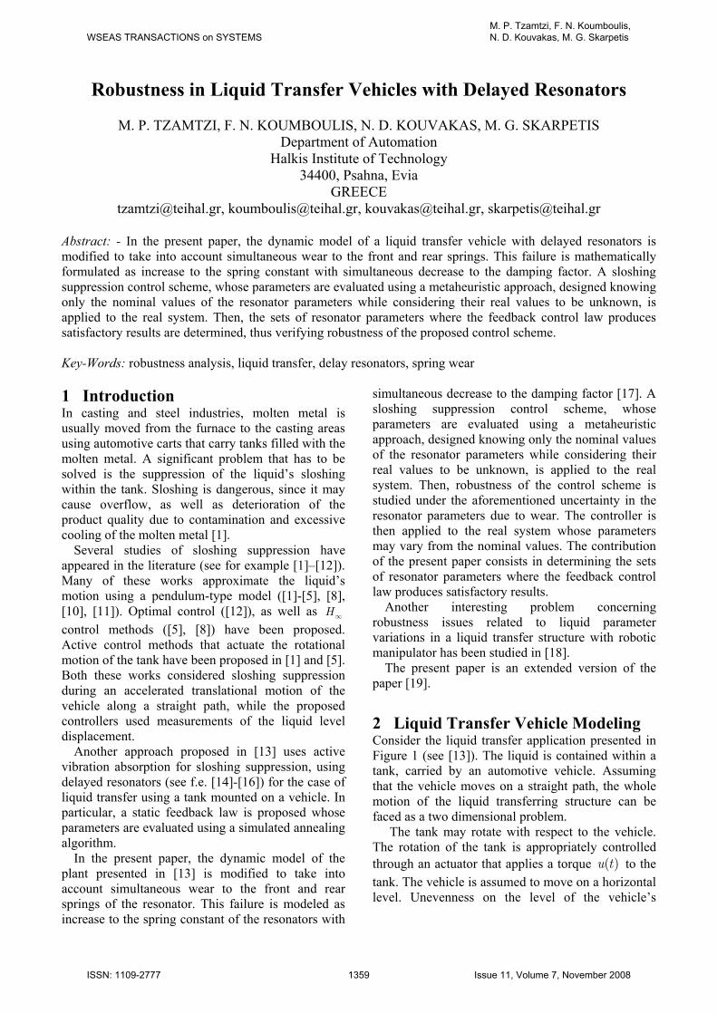
res resc c= . With respect to efficiency of the search algorithm, it has been observed that it had converged to the controller parameters after 9000 repetitions. Nevertheless, it must be noted that the search algorithm thresholds are quite strict and the controller has practically converged much sooner while the closed loop performance response remains practically unchanged. Indicatively, in Table 1 the center values and half widths of the controller parameters are presented. Indeed, it can be observed that the response characteristics remain practically unchanged after the fourth loop. Note that the all response parameters are evaluated using the sampled data.

Repetition 1,cf

2,cf

4,cf

1,wf

2,wf

3,wf Cost

1 -57.1415 -9.08794 -0.02713 32.80708 1.897013 0.125018 98.26337 2 -58.9868 -9.72769 -0.03088 9.718936 1.147686 0.048136 89.69127 3 -67.6406 -10.7424 -0.01881 5.473802 0.637211 0.022937 86.66839 4 -72.8916 -11.2102 -0.02078 0.677065 0.038506 0.00561 85.62089 5 -73.0781 -11.2468 -0.01894 0.036232 0.020287 0.000604 85.57291 6 -73.108 -11.2659 -0.01947 0.020413 0.00282 3.08E-05 85.55719 7 -73.1283 -11.2687 -0.01944 0.000218 0.0013 4.64E-05 85.55463 8 -73.1285 -11.27 -0.01941 2.26E-05 0.000114 3.33E-05 85.55422 9 -73.1286 -11.2701 -0.01938 1.98E-06 1.33E-05 9.22E-06 85.55416

Table 1: Metaheuristic Algorithm Parameters and Closed Loop Cost Criterion

To demonstrate the performance of the proposed control scheme, consider the nonlinear model (2.1)

and the data presented previously, assuming that 0

reskδ = and 0

rescδ = . In Figures 3 to 14 the



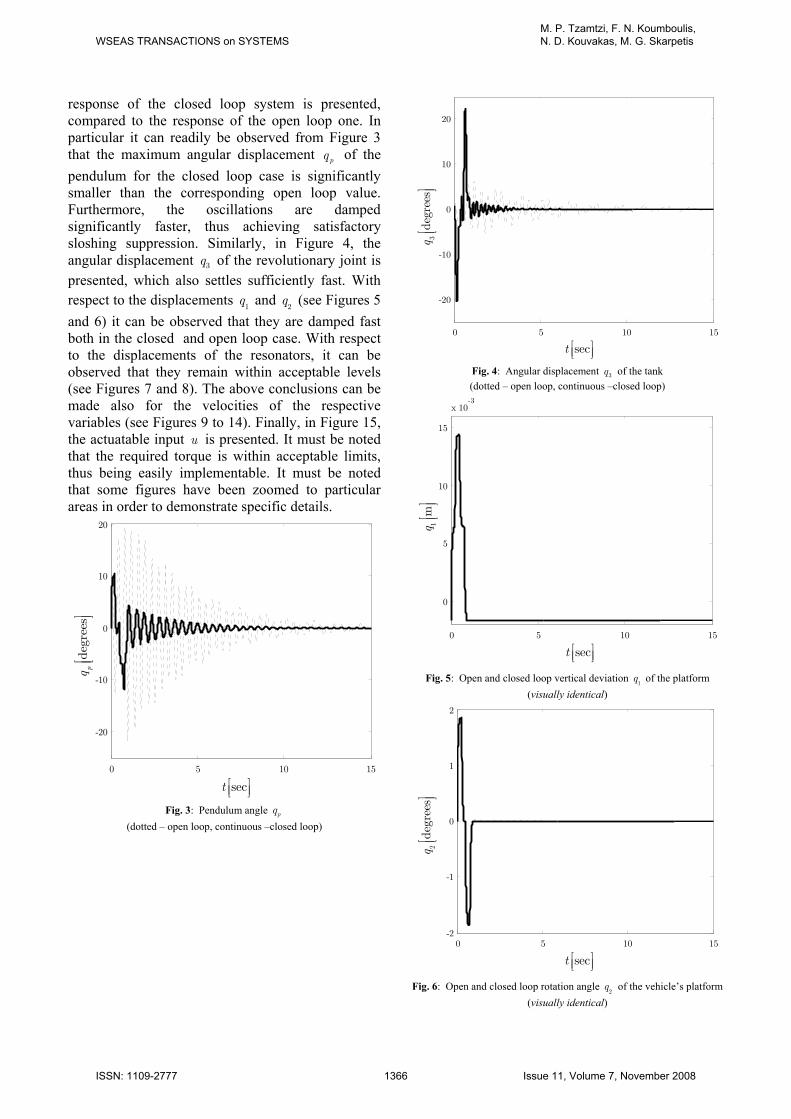
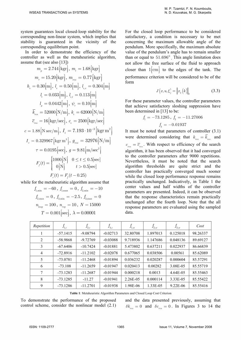
response of the closed loop system is presented, compared to the response of the open loop one. In particular it can readily be observed from Figure 3 that the maximum angular displacement pq of the pendulum for the closed loop case is significantly smaller than the corresponding open loop value. Furthermore, the oscillations are damped significantly faster, thus achieving satisfactory sloshing suppression. Similarly, in Figure 4, the angular displacement 3q of the revolutionary joint is presented, which also settles sufficiently fast. With respect to the displacements

1q and

2q (see Figures 5

and 6) it can be observed that they are damped fast both in the closed and open loop case. With respect to the displacements of the resonators, it can be observed that they remain within acceptable levels (see Figures 7 and 8). The above conclusions can be made also for the velocities of the respective variables (see Figures 9 to 14). Finally, in Figure 15, the actuatable input u is presented. It must be noted that the required torque is within acceptable limits, thus being easily implementable. It must be noted that some figures have been zoomed to particular areas in order to demonstrate specific details.

0 5 10 15

-20

-10

0

10

20

deg

rees

pq⎡

⎤⎢

⎥⎣

⎦

sect ⎡ ⎤⎢ ⎥⎣ ⎦ Fig. 3: Pendulum angle pq

(dotted – open loop, continuous –closed loop)

3de

gree

sq

⎡⎤

⎢⎥

⎣⎦

sect ⎡ ⎤⎢ ⎥⎣ ⎦

0 5 10 15

-20

-10

0

10

20

Fig. 4: Angular displacement 3q of the tank (dotted – open loop, continuous –closed loop)

1m

q⎡

⎤⎢

⎥⎣

⎦

sect ⎡ ⎤⎢ ⎥⎣ ⎦

0 5 10 15

0

5

10

15

x 10-3

Fig. 5: Open and closed loop vertical deviation 1q of the platform

(visually identical)

2de

gree

sq

⎡⎤

⎢⎥

⎣⎦

sect ⎡ ⎤⎢ ⎥⎣ ⎦

0 5 10 15-2

-1

0

1

2

Fig. 6: Open and closed loop rotation angle

2q of the vehicle’s platform




max⎡

⎤⎢

⎥⎣

⎦

sect ⎡ ⎤⎢ ⎥⎣ ⎦

0 0.5 1 1.5 2 2.5

0

5

10

x 10-3

Fig. 7: Open and closed loop front resonator deviation

ax


mbx⎡

⎤⎢

⎥⎣

⎦

sect ⎡ ⎤⎢ ⎥⎣ ⎦

0 0.5 1 1.5 2 2.5

0

5

10

x 10-3

Fig. 8: Open and closed loop rear resonator deviation bx


degr

ees/

sec

pq⎡

⎤⎢

⎥⎣

⎦

sect ⎡ ⎤⎢ ⎥⎣ ⎦

0 5 10 15-400

-200

0

200

400

Fig. 9: Pendulum angle velocity pq


3de

gree

s/se

cq

⎡⎤

⎢⎥

⎣⎦

sect ⎡ ⎤⎢ ⎥⎣ ⎦

0 5 10 15-300

-200

-100

0

100

200

300

400

Fig. 10: Angular displacement velocity

3q of the tank


1m

/sec

q⎡

⎤⎢

⎥⎣

⎦

sect ⎡ ⎤⎢ ⎥⎣ ⎦

0 0.5 1 1.5 2 2.5-0.2

-0.1

0

0.1

0.2

Fig. 11: Open and closed loop vertical deviation velocity

1q of the

platform (visually identical)

2de

gree

s/se

cq

⎡⎤

⎢⎥

⎣⎦

sect ⎡ ⎤⎢ ⎥⎣ ⎦

0 0.5 1 1.5 2 2.5-50

0

50

Fig. 12: Open and closed loop rotation angle velocity

2q of the

vehicle’s platform (visually identical)



m/s

ecax⎡

⎤⎢

⎥⎣

⎦

sect ⎡ ⎤⎢ ⎥⎣ ⎦

0 0.5 1 1.5 2 2.5-0.8

-0.6

-0.4

-0.2

0

0.2

0.4

0.6

Fig. 13: Open and closed loop front resonator deviation velocity

ax (visually identical)

m/s

ecbx⎡

⎤⎢

⎥⎣

⎦

sect ⎡ ⎤⎢ ⎥⎣ ⎦

0 0.5 1 1.5 2 2.5-0.8

-0.6

-0.4

-0.2

0

0.2

0.4

0.6

Fig. 14: Open and closed loop rear resonator deviation velocity

bx (visually identical)

Nm

u⎡

⎤⎢

⎥⎣

⎦

sect ⎡ ⎤⎢ ⎥⎣ ⎦

0 5 10 15

-2

-1

0

1

2

Fig. 15: Actuatable input u

4 Robustness Analysis of the Closed Loop System The robustness of the closed loop system will be examined for the following range of uncertainty:

13.6,res resc cδ ⎡ ⎤∈ ⎢ ⎥⎣ ⎦ and , 59800

res resk kδ ⎡ ⎤∈ ⎢ ⎥⎣ ⎦ .

Assuming that this limitation holds, the robustness of the closed loop system in each case will be examined using the following cost criteria

( ) ( )21

0

,res res p

f k c q t dtδ δ∞

= ∫ (4.1a)

( ) ( )22 3

0

,res res

f k c q t dtδ δ∞

= ∫ (4.1b)

The integrals in criteria (4.1) are guaranteed to converge to some value. This is because the steady state values of ( )p

q t and ( )3q t are equal to zero.

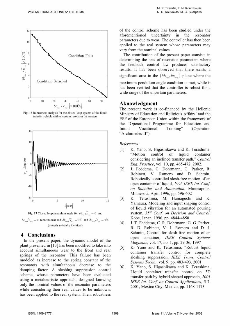
Using simulation results for several values of the uncertain parameters, we determine an area of the ( ),

res resk cδ δ plane where the maximum pendulum

angle condition is met. This area is presented in Figure 16. From Figure 16 it can be observed that this area covers a significant range in the ( ),

res resk cδ δ plane. Hence, it is verified that

controller (3.1) is indeed robust. This can also be verified by the cost criteria (4.1). Indeed, using the simulation results, it can be observed that for those values of the uncertain parameters that lie within the area where the maximum pendulum angle condition is met, the corresponding values of the cost criteria introduced in (4.1), do not significantly change. Finally in Figure 17, the closed loop pendulum angle response is presented for the cases a) 0

reskδ = and

0rescδ = and b) 9%

res resk kδ = and

9%res resc cδ = . Note that the second case is

marginally inside the area where the maximum pendulum angle condition is satisfied. It can be observed that the two responses are visually identical. The same observation holds for all ( ),

res resk cδ δ where the maximum pendulum angle

condition is satisfied. This is consistent with the fact that the cost criteria (4.1a) and (4.1b) do not significantly change inside that area.



/10

0%res

res

kk

δ⎡

⎤× ⎢

⎥⎣

⎦

/ 100%res resc cδ ⎡ ⎤×⎢ ⎥⎣ ⎦

0 10 20 30 40 50 600

2

4

6

8

10

12

Condition Satisfied

Condition Fails

Fig. 16 Robustness analysis for the closed-loop system of the liquid

transfer vehicle with uncertain resonator parameters

deg

rees

pq⎡

⎤⎢

⎥⎣

⎦

sect ⎡ ⎤⎢ ⎥⎣ ⎦

0 5 10 15-15

-10

-5

0

5

10

15

Fig. 17 Closed loop pendulum angle for 0res resk kδ = and

0res resc cδ = (continuous) and 9%

res resk kδ = and 9%

res resc cδ =

(dotted) (visually identical)

4 Conclusions In the present paper, the dynamic model of the

plant presented in [13] has been modified to take into account simultaneous wear to the front and rear springs of the resonator. This failure has been modeled as increase to the spring constant of the resonators with simultaneous decrease to the damping factor. A sloshing suppression control scheme, whose parameters have been evaluated using a metaheuristic approach, designed knowing only the nominal values of the resonator parameters while considering their real values to be unknown, has been applied to the real system. Then, robustness

of the control scheme has been studied under the aforementioned uncertainty in the resonator parameters due to wear. The controller has then been applied to the real system whose parameters may vary from the nominal values.

The contribution of the present paper consists in determining the sets of resonator parameters where the feedback control law produces satisfactory results. It has been observed that there exists a significant area in the ( ),

res resk cδ δ plane where the

maximum pendulum angle condition is met, while it has been verified that the controller is robust for a wide range of the uncertain parameters.

Aknowledgment The present work is co-financed by the Hellenic Ministry of Education and Religious Affairs’ and the ESF of the European Union within the framework of the “Operational Programme for Education and Initial Vocational Training” (Operation “Archimedes-II”). References [1] K. Yano, S. Higashikawa and K. Terashima,

“Motion control of liquid container considering an inclined transfer path,” Control Eng. Practice, vol. 10, pp. 465-472, 2002.

[2] J. Feddema, C. Dohrmann, G. Parker, R. Robinett, V. Romero and D. Schmitt, Robotically controlled slosh-free motion of an open container of liquid, 1996 IEEE Int. Conf. on Robotics and Automation, Minneapolis, Minnesota, April 1996, pp. 596-602

[3] K. Terashima, M, Hamaguchi and K. Yamaura, Modeling and input shaping control of liquid vibration for an automated pouring system, 35th Conf. on Decision and Control, Kobe, Japan, 1996, pp. 4844-4850

[4] J. T. Feddema, C. R. Dohrmann, G. G. Parker, R. D. Robinett, V. J. Romero and D. J. Schmitt, Control for slosh-free motion of an open container, IEEE Control Systems Magazine, vol. 17, no. 1, pp. 29-36, 1997

[5] K. Yano and K. Terashima, “Robust liquid container transfer control for complete sloshing suppression, IEEE Trans. Control Systems Techn., vol. 9, pp. 483-493, 2001

[6] K. Yano, S. Higashikawa and K. Terashima, Liquid container transfer control on 3D transfer path by hybrid shaped approach, 2001 IEEE Int. Conf. on Control Applications, 5-7, 2001, Mexico City, Mexico, pp. 1168-1173



[7] K. Yano, T. Toda and K. Terashima, Sloshing suppression control of automatic pouring robot by hybrid shape approach, 40th IEEE Conference on Decision and Control, Orlando, Florida, USA, December 2001, pp. 1328-1333

[8] K. Terashima and K. Yano, Sloshing analysis and suppression control of tilting-type automatic pouring machine, Control Eng. Practice, vol. 9, pp. 607-620, 2001

[9] H. Sira-Ramirez, A flatness based generalized PI control approach to liquid sloshing regulation in a moving container, American Control Conference, Anchorage, USA, May 8-10, 2002, pp. 2909-2914

[10] S. Kimura, M. Hamaguchi and T. Taniguchi, Damping control of liquid container by a carrier with dual swing type active vibration reducer, 41st SICE Annual Conference, 2002, pp. 2385- 2388.

[11] Y. Noda, K. Yano and K. Terashima, Tracking to moving object and sloshing suppression control using time varying filter gain in liquid container transfer, 2003 SICE Annual Conference, Fukui, Japan, 2003, pp. 2283-2288

[12] M. Hamaguchi, K. Terashima, H. Nomura, Optimal control of liquid container transfer for several performance specifications, J. Advanced Autom. Techn., vol. 6, pp. 353-360, 1994

[13] M.P. Tzamtzi, F.N. Koumboulis, N.D. Kouvakas and G.E. Panagiotakis, A Simulated Annealing Controller for Sloshing Suppression in Liquid Transfer with Delayed Resonators, 14th Mediterranean Conf. on Control and Autom., Ancona, Italy, June 2006.

[14] N. Olgac and B. T. Holm-Hansen, A novel active vibration technique: delayed resonator, Journal of Sound and Vibration, vol. 176, no. 1, pp. 93-104, 1994

[15] N. Olgac, H. Elmali and S. Vijayan, Introduction to the dual frequency delayed resonator, Journal of Sound and Vibration, vol. 189, no. 3, pp. 355-367, 1996

[16] D. Filipovic, N. Olgak, Delayed resonator with speed feedback including dual frequency - theory and experiments, 36th Conf. on Decision and Control, San Diego, California, USA, Dec. 1997, pp. 2535-2540

[17] O. Buyukozturk and T.-Y. Yu, Structural Health Monitoring and Seismic Impact Assessment, 5th National Conf on Earthquake Engineering, Istanbul, Turkey, May 2003

[18] M.P. Tzamtzi, F.N. Koumboulis, Robustness of a Robot Control Scheme for Liquid Transfer, Int. Joint Conf. on Comp., Information, and Systems Sciences, and Eng. (CIS2E 07), Dec. 2007 // also in Novel Algorithms and Techniques in Telecommunications, Automation and Industrial Electronics, T. Sobh et al. (eds), pp. 154-161, Springer, 2008

[19] M. P. Tzamtzi, F. N. Koumboulis, N.D. Kouvakas, M.G. Skarpetis, “Robustness in Liquid Transfer Vehicles with Delayed Resonators”, 6th WSEAS International Conference on Circuit, Systems, Electronics, Control & Signal Processing (CSECS'07), pp. 233-238

[20] F.N. Koumboulis and M.P. Tzamtzi, A metaheuristic approach for controller design of multivariable processes, pp 1429-1432, 12th IEEE International Conference on Emerging Technology on Factory Automation, Rio-Patras, Greece 2007

[21] N.D. Kouvakas N.D. Kouvakas, F.N. Koumboulis and P.N. Paraskevopoulos, Modeling and Control of a Test Case Central Heating System, 6th WSEAS International Conference on Circuits, Systems, Electronics, Control & Signal Processing, Cairo-Egypt, 2007. pp. 289-297

[22] M. P. Tzamtzi, F. N. Koumboulis, M.G. Skarpetis, “On the Controller Design for the Outpouring Phase of the Pouring Process”, 6th WSEAS International Conference on Circuits, Systems, Electronics, Control & Signal Processing (CSECS'07), Cairo, Egypt, 2007, pp. 270-277.

[23] M.R. Jalali, A. Afshar, M.A. Marino, “Ant Colony Optimization Algorithm (ACO); A New Heuristic Approach for Engineering Optimization”, 6th WSEAS International Conference on Evolutionary Computing, Lisbon, Portugal, June 16-18, 2005, pp. 188-192.



Documents

Robustness in Liquid Transfer Vehicles with … in Liquid Transfer Vehicles with Delayed Resonators M. P. TZAMTZI, F. N. KOUMBOULIS, N. D. KOUVAKAS, M. G. SKARPETIS Department of Automation