Robustness and Pricing with UncertainGrowth

Marco Cagetti, Lars Peter Hansen, Thomas Sargent and

Noah Williams1

October 12, 2001

Abstract. We study how decision makers’ concerns about robustness affect prices andquantities in a stochastic growth model. In the model economy, growth rates in technologyare altered by infrequent large shocks and continuous small shocks. An investor observesmovements in the technology level but cannot perfectly distinguish their sources. Insteadthe investor solves a signal extraction problem. We depart from most of the macroeco-nomics and finance literature by presuming that the investor treats the specification oftechnology evolution as an approximation. To promote a decision rule that is robust tomodel misspecification, an investor acts as if a malevolent player threatens to perturbthe actual data generating process relative to his approximating model. We study howa concern about robustness alters asset prices. We show that the dynamic evolution ofthe risk-return tradeoff is dominated by movements in the growth-state probabilities andthat the evolution of the dividend-price ratio is driven primarily by the capital-technologyratio.

1 Introduction

This paper shows how decision makers’ concerns about model misspecification can affectprices and quantities in a dynamic economy. We use the familiar stochastic growth modelof Brock and Mirman (1972) and Merton (1975) as a laboratory. Technology is specifiedas a continuous-time hidden Markov model (HMM), inducing investors to make inferencesabout the growth rate. They form their opinions about the growth rate from current andpast observations of technology that are clouded by concurrently evolving small shocks

1Lars Peter Hansen: Department of Economics, University of Chicago (l-hansen@uchicago.edu).Thomas Sargent: Department of Economics, Stanford University (sargent@leland.stanford.edu).Marco Cagetti: Department of Economics, University of Virginia (cacio@virginia.edu). NoahWilliams: Department of Economics, Princeton University (noahw@princeton.edu). Commentsfrom John Heaton, Pascal Maenhout and Grace Tsiang are gratefully acknowledged. Both Hansenand Sargent were supported by the National Science Foundation while completing this project.

1

modelled as Brownian motions. We show how investors’ desire to make their decisionrules robust to misspecification of the evolution of technology alters security prices andthe intertemporal resource allocation.

Following the control theory literature, we formulate the robust decision-making pro-cess as a two-player game. For a game-theoretic approach to robust decision-making seeBasar and Bernhard (1995). For the recursive specification used here see Cagetti, Hansen,Sargent, and Williams (2000). An investor has somehow constructed a model of the tech-nology shock process, but suspects that model to be misspecified. The investor wants tomaximize the expected value of a discounted utility function, but doubting his approxi-mating model, is unsure about what probability distribution to use to form mathematicalexpectations. To make decisions that perform well under a variety of models, the decisionmaker imagines that a second malevolent agent will draw technology shocks from a modelthat is distorted relative to his approximating model. The malevolent agent minimizes thedecision maker’s objective function by choosing a model from a large set surrounding theapproximating model. To represent the idea that the decision maker views his model as agood approximation, we restrict the surrounding models to be close to the approximatingmodel, where closeness is measured by a statistical discrimination criterion of the gapbetween a distorted model and the approximating model.2

The malevolent agent in the decision problem provides an operational way to promoterobustness by systematically exploring the types of model misspecification to which aproposed decision rule is especially fragile.3 As argued by Huber (1981) in his discussionof an optimal robust statistical procedure:

... as we defined robustness to mean insensitivity with regard to small devi-ations from assumptions, any quantitative measure of robustness must some-how be concerned with the maximum degradation of performance possible foran ε-deviation from the assumptions. The optimally robust procedure mini-mizes this degradation and hence will be a minimax procedure of some kind.

In this paper, we model investor preferences using a penalty approach that lets in-vestors explore deviations from an approximating model of the technology evolution.4

2As is typical with rational expectations models, we do not explore formally how investors arriveat an approximating model, but we do presume that the remaining models that are entertained aredifficult to distinguish from the approximating model given historical data. A rational expectationscounterpart model, however, would remove model approximation error from consideration.

3Economists use a max-min formulation when they use Lagrange multipliers. Lagrange mul-tipliers allow us to convert a constrained maximization problem into an unconstrained max-minproblem. The constraint is imposed by supposing there exists a fictitious malevolent agent whoseaim it is to punish the original decision-maker when the constraint is violated. This device forimposing a constraint is algorithmically convenient. So is our two-agent formulation of robustness.

4Although we use ideas from standard robust control theory, we modify them because our ap-proximating models are stochastic. Among the few examples of stochastic robust control modelsare James (1992), who studies deterministic differential games of robust decision-making as smallnoise limits, and Dupuis, James, and Petersen (1998). A stochastic approximating model is essen-

2

Formally, we append a term to the discounted expected utility that penalizes departuresfrom a reference or approximating model. Penalty methods are common in both therobust control theory and the statistics literatures. Strictly speaking they imply prefer-ences that are distinct from those that limit exploration only to ε-deviations as suggestedby Huber (1981) in the above quote, but the two approaches are related. (For exam-ple see Dupuis, James, and Petersen (1998) and Hansen, Sargent, Turmuhambetova, andWilliams (2001).) We use a penalty function that tolerates only perturbations from theapproximating model that are difficult to detect statistically. This leads us to use alog-likelihood-ratio-based penalty term called relative entropy, appropriately adjusted toaccount for the HMM structure.5

Concern about model misspecification makes investors more cautious and enlargesmeasured risk premia. It enhances the usual precautionary motive.6

Our model economy is a continuous-time stochastic growth economy. The technologyshock process has a two-state hidden Markov (HMM) structure. Our quantitative esti-mates confirm the findings of Hamilton (1989) and others that a two-state HMM modelfor the post World War II U.S. recovers states that measure short recessions and sustainedbooms. Because it can be difficult to distinguish these two states from the observed tech-nology level, we investigate the consequences of concealing the growth state from thedecision-maker. Our specification of the technology shock process formally follows Won-ham (1964), David (1997), and Veronesi (1999). The latter two papers study pricing inproduction economies with linear technologies and hidden dividend growth processes.7

Hidden information gives us a tractable setting to study what happens when the qualityof investors’ information fluctuates over time. This mechanism alone can alter the timeseries evolution of the market risk prices and dividend price ratios, but it cannot producelarge enough risk premia to be empirically plausible. It is for this reason that we turn torobustness as a means of changing asset price predictions.

We decentralize the robust version of the stochastic growth model by computingshadow prices from a robust resource allocation problem. The continuous-time specifi-cation lets us use representations of local prices to assemble asset prices for intervals oftime. The local prices include both the instantaneous interest rate and the risk price ofthe Brownian motion increment. Our model contributes an additional component of thefactor risk price that is attributable to a concern about model misspecification. This com-ponent also occurs in the continuous-time papers of Anderson, Hansen, and Sargent (2000)

tial for our application to finance. In emphasizing this structure, we follow Hansen, Sargent, andTallarini (1999), Anderson, Hansen, and Sargent (2000), and Maenhout (1999).

5Examples of robust control of deterministic systems with partial observations are James, Baras,and Elliott (1994) and James and Baras (1996).

6The precautionary motive is already present in models without quadratic preferences.7David (1997) studies a model in which production is linear in the capital stocks with technology

shocks that have hidden growth rates. Veronesi (1999) studies a permanent income model witha riskless linear technology. Dividends are modelled as an additional consumption endowment.Hidden information was introduced into asset pricing models by Detemple (1986), who considersa production economy with Gaussian unobserved variables.

3

and Chen and Epstein (2001), and as an approximation in the discrete-time analysis ofHansen, Sargent, and Tallarini (1999).

Quantitatively, our two-state HMM specification has the following implications forintertemporal prices and allocations. The investor’s signal extraction problem makes onestate variable be the probability that the current growth rate is low. Another state variableis the ratio of capital to technology. We show that:

• The robust motive for precautionary savings increases the capital stock. This motivecan be offset by making investors discount the future more.

• A concern about model misspecification adds a quantitatively important componentto the risk-return tradeoff as measured by financial econometricians. The componentof risk prices due to robustness is particularly sensitive to growth-state probabilitiesand is largest when, under the approximating model, investors are most unsure ofthe hidden state.

• A concern about robustness causes price-dividend ratios to drop closer to the levelobserved in post war data. In our model economy, these ratios are particularlysensitive to movements in capital/technology ratio. They respond very little tochanges in the growth-state probabilities. The actual time series trajectories forprice-earnings ratios differ substantially from those implied by the model.

The first finding extends a result of Hansen, Sargent, and Tallarini (1999) to a nonlineareconomy. Without prior information about the subjective discount factor, decision mak-ers’ concerns about robustness can’t be detected from macroeconomic quantities alone.The second two findings have important counterparts in a corresponding HMM rationalexpectation economy in which investors only care about risk. In such economies, marketrisk prices respond primarily to changes in growth-state probabilities while dividend-priceratios are driven primarily by movements in the capital/technology ratio.

The paper is structured as follows. Section 2 presents the economic environment. Sec-tion 3 describes the information structure and the signal extraction problem. Section 4describes model distortions and measures of model misspecification. Section 5 presentsdifferential equations for value functions that characterize equilibria of the hidden infor-mation games. Section 6 discusses implications for time series of capital stocks. Section 7uses the link between statistical detection and robustness to restrict the degree of robust-ness in the asset calculations. Section 8 shows how risk-return tradeoffs change over time.Section 9 displays the implied dividend-price ratios.

2 The economy

We use a continuous-time formulation of a Brock and Mirman (1972) economy with pro-duction, capital accumulation, and stochastic productivity growth. There are two typesof technology shocks: Brownian motion increments, and infrequent changes in the drifts

4

of the Brownian motion modelled as a jump process. Investors observe productivity levelsbut the drift is hidden. The technology process is thus a special case of a HMM, con-fronting investors with a signal extraction problem. Current and past data must be usedto make inferences about technological growth.

We use this model to study:

• the precautionary motive for savings induced by a concern about robustness;

• the evolution of the measured market price of ‘risk’;

• the evolution of price-dividend ratios.

2.1 Previous literature

The quantitative component of our investigation is designed to show how robustness altersthe implications of the simple growth model familiar to economists. In the absence ofrobustness, the empirical implications of this model for consumption and investment aredefective (e.g. see Watson (1993)) and the implied return to capital shows very littlevariation relative, for instance, to valued-weighted returns on equity (e.g. see Cochrane(1991) and Rouwenhorst (1995)). The absence of return variability is even more stark inthe continuous-time embedding of this model. As noted by Merton (1975), the return tocapital becomes locally riskless.

One remedy is to make capital locally risky. While this will enhance return vari-ability, it may also result in excessive volatility in aggregate quantities. In addition, wemight follow Boldrin, Christiano, and Fisher (1999) and others by introducing additionaltechnological frictions and temporal nonseparabilities in preferences. Instead of mixingrobustness with these other ways to complicate the short run dynamics, we study the roleof robust decision-making in a simpler framework.

When looking at the asset pricing implications, we will be less ambitious than Boldrin,Christiano, and Fisher (1999) and Hansen and Singleton (1983),8 and will study only thelocal or instantaneous risk-return relation and the time series behavior for dividend priceratios. Even the risk-return relation looks puzzling for a model without robust decision-makers because the implied market price is too small to be plausible from the vantagepoint of aggregate models (Hansen and Jagannathan (1991) and Cochrane and Hansen(1992)). As in Hansen, Sargent, and Tallarini (1999), Anderson, Hansen, and Sargent(2000), Chen and Epstein (2001) and Maenhout (1999), we explore the effects of a concernabout model uncertainty on the measured risk premium in security market returns. Weadd to this literature by looking at the time series variation both of risk prices and ofmodel uncertainty prices. We show how disguising mean growth rates from investors canalter the time series properties of the risk premia.

To study dividend-price ratios we will eventually posit an exogenous dividend claimthat is distinct from the marginal product of capital. In this we imitate Veronesi (2000)

8We look at only a subset of the restrictions that they studied.

5

and David and Veronesi (1999) except that we have an additional state variable (capital)and also explore implications for robustness.

2.2 Technology

We assume a Cobb-Douglas production function

f(K, L) = Kα(Y L)1−α

where K is the capital stock, L is the labor supply and Y is the labor-augmenting technol-ogy parameter. For simplicity, we fix the total labor supply L at 1. Y evolves exogenouslyaccording to the continuous-time process

dyt = st · κ dt + σydBt (1)

where B is a standard Brownian motion, y = log Y , and s evolves according to a finite-state Markov chain. It can assume n possible values, U1, U2, ..., Un, where Uj is a vectorcontaining 1 in position j and zero everywhere else. κ is an n-dimensional vector thatcontains all possible values of the mean growth rate of the technology shock; sj · κ istherefore the growth rate in state j. The model of the technology shock can be viewedas a continuous-time embedding of the regime-shift models of Baum and Petrie (1966),Sclove (1983) and Hamilton (1989).9

Let δ be the depreciation rate of capital. The evolution equation for capital is givenby:

dKt = [(Yt)1−α(Kt)α − Ct − δKt]dt (2)

where Ct is the instantaneous consumption flow. By construction, capital is locally pre-dictable.

The technological process has a unit root in logarithms and is therefore nonstationary.As we show later, the ratio of capital to effective labor, kt = Kt/Yt and that of consumptionto effective labor, ct = Ct/Yt, are stationary. We will therefore represent the problem interms of the variables kt and yt.

Applying Ito’s lemma, we get

dkt = µk(c, k, s)dt + σk(k)dBt (3)

where the drift of (3) is

µk(c, k, s) ≡ kα − c −[s · κ + δ − (σy)2

2

]k

9An important qualification is that volatility is independent of the Markov chain state. Thuswe are ruling a process with high volatility in low growth or recession states. Baum and Petrie(1966) and Bonomo and Garcia (1996) allow for the state st to alter volatility and find it to beempirically plausible for postwar output data and century long consumption data. We precludethis dependence in order that our state st remain difficult to detect from high frequency data.Volatility changes are revealed by continuous data records.

6

and the local standard deviation is:

σk(k) = −σyk.

2.3 Evolution of technology growth states

The finite-state Markov chain for s has an intensity matrix

A = N(Q − I)

where N is a diagonal matrix of jump intensities, each of which dictates the jump frequencyconditioned on the current state. We let ηi denote the jump intensity for state i. Thematrix Q is a transition matrix. Each row specifies the probability distribution of thejump location conditioned on a jump taking place. We normalize the transition matrix Qso that its {i, i} entry is zero. That is, conditioned on a jump from state i taking place,there is no chance that the state will remain the same.10 The element {i, j} of A will bedenoted by aij , and ai,i = −

∑j,j 6=i aij .

The transition probabilities over any interval of time can be constructed from theintensity matrix A via the exponential formula:

Tτ = exp(τA) (4)

and the intensity matrix can be deduced from the transition matrices by computing theright derivative of Tτ at τ = 0.

3 The hidden information problem

We consider models in which the mean growth rate st · κ is hidden to investors. Thus theymust solve a signal extraction problem by using past levels of technology shock incrementsto forecast mean growth rates. Before solving the stochastic growth model under thealternative games, we display the solution to the signal extraction problem. A separationproperty of recursive prediction and control in our resource allocation games allows usfirst to solve the signal extraction problem using the approximating model and then touse the filtering equations as an input into the solution of the games. The details of thedecision problem that justifies separation are described in Cagetti, Hansen, Sargent, andWilliams (2000).

10There are other normalizations that might be adopted. For instance, we could make thejump intensity constant across states, provided that conditioned on a jump taking place, thereis a positive probability of remaining in the same state. The constant intensity specification issometimes used because it simplifies the characterization of the stationary distribution.

7

3.1 General formulation

Since the state variable s is not observed, the decision maker has to infer information aboutthe current state of the system by using the current and the past observations of y. Thishidden state model is due to Wonham (1964), and is described in Liptser and Shiryayev(1977) and Elliott, Aggoun, and Moore (1995). It has been used in asset-pricing modelsby David (1997), Veronesi (1999), Veronesi (2000) and David and Veronesi (1999).

The expected value of the drift of y, st · κ, given the current information is κt = κ · pt.The n-dimensional vector pt contains the probabilities of being in each of the states, giventhe information set at time t {Yt : t ≥ 0}. These conditional probabilities evolve accordingto the stochastic differential equation:

dpt = A′ptdt + σp(pt)dBt (5)

σp(p) =1σy

P (I − 1np′)κ

where P is a matrix with the elements of p on the diagonal. The normalized innovationprocess dBt containing the new information used to generate Yt is:

dBt =1σy

(dyt − κ · stdt) = dBt +κ · (st − pt)

σydt. (6)

The evolution of the technology shock under the innovation process B is:

dyt = κ · ptdt + σydBt (7)

and the evolution of k is:

dkt = µ(ct, kt, pt)dt + σk(k)dBt (8)

where

µ(c, k, p) = kα − c −[κ · p + δ − (σy)2

2

]k.

3.2 The two-state case

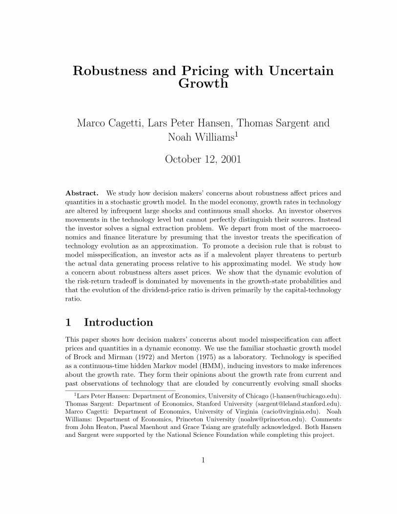
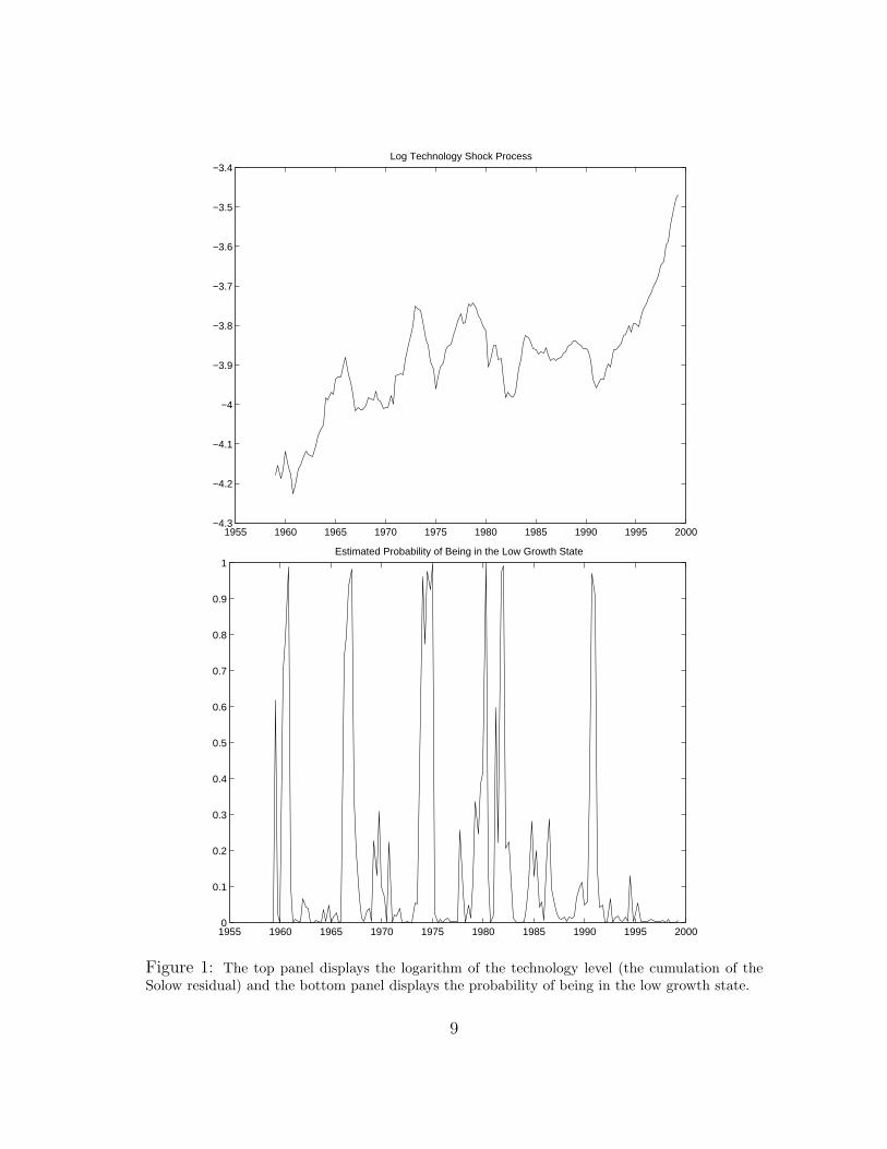
We consider in particular the case in which the state st can assume two values, corre-sponding to a positive growth rate κ1 in expansions and a negative growth rate κ2 inrecessions. The technology shock process is shown in the top panel of Figure 1, and thebottom panel plots the estimated probabilities of being in the low growth state computedusing our baseline estimates. Under our approximating model, the post WWII experiencewas one characterized by sharp recessions and extended expansions. Although we use thisspecification as a model of the technology process, it mirrors that used by Hamilton (1989)in his study of output growth.

8

1955 1960 1965 1970 1975 1980 1985 1990 1995 2000−4.3

−4.2

−4.1

−4

−3.9

−3.8

−3.7

−3.6

−3.5

−3.4Log Technology Shock Process

1955 1960 1965 1970 1975 1980 1985 1990 1995 20000

0.1

0.2

0.3

0.4

0.5

0.6

0.7

0.8

0.9

1Estimated Probability of Being in the Low Growth State

Figure 1: The top panel displays the logarithm of the technology level (the cumulation of theSolow residual) and the bottom panel displays the probability of being in the low growth state.

9

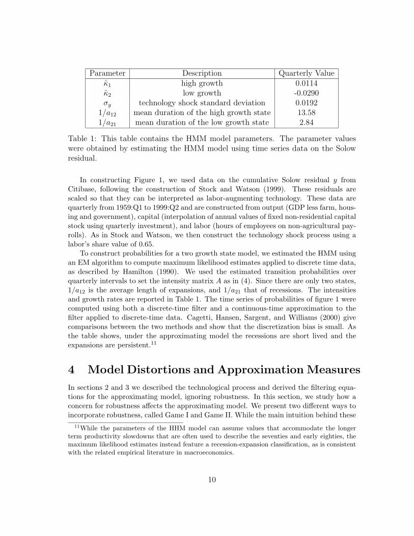
Parameter Description Quarterly Valueκ1 high growth 0.0114κ2 low growth -0.0290σy technology shock standard deviation 0.0192

1/a12 mean duration of the high growth state 13.581/a21 mean duration of the low growth state 2.84

Table 1: This table contains the HMM model parameters. The parameter valueswere obtained by estimating the HMM model using time series data on the Solowresidual.

In constructing Figure 1, we used data on the cumulative Solow residual y fromCitibase, following the construction of Stock and Watson (1999). These residuals arescaled so that they can be interpreted as labor-augmenting technology. These data arequarterly from 1959:Q1 to 1999:Q2 and are constructed from output (GDP less farm, hous-ing and government), capital (interpolation of annual values of fixed non-residential capitalstock using quarterly investment), and labor (hours of employees on non-agricultural pay-rolls). As in Stock and Watson, we then construct the technology shock process using alabor’s share value of 0.65.

To construct probabilities for a two growth state model, we estimated the HMM usingan EM algorithm to compute maximum likelihood estimates applied to discrete time data,as described by Hamilton (1990). We used the estimated transition probabilities overquarterly intervals to set the intensity matrix A as in (4). Since there are only two states,1/a12 is the average length of expansions, and 1/a21 that of recessions. The intensitiesand growth rates are reported in Table 1. The time series of probabilities of figure 1 werecomputed using both a discrete-time filter and a continuous-time approximation to thefilter applied to discrete-time data. Cagetti, Hansen, Sargent, and Williams (2000) givecomparisons between the two methods and show that the discretization bias is small. Asthe table shows, under the approximating model the recessions are short lived and theexpansions are persistent.11

4 Model Distortions and Approximation Measures

In sections 2 and 3 we described the technological process and derived the filtering equa-tions for the approximating model, ignoring robustness. In this section, we study how aconcern for robustness affects the approximating model. We present two different ways toincorporate robustness, called Game I and Game II. While the main intuition behind these

11While the parameters of the HHM model can assume values that accommodate the longerterm productivity slowdowns that are often used to describe the seventies and early eighties, themaximum likelihood estimates instead feature a recession-expansion classification, as is consistentwith the related empirical literature in macroeconomics.

10

two representations is similar, each of them analyzes different ways in which the approxi-mating model can be perturbed. Then, in subsection 4.4, as a benchmark we also describethe full information robustness case, where the growth state s is perfectly observed (andthus there is no filtering problem), but the decision maker still entertains the possibilitythat the approximating model describing the technological process is misspecified.

4.1 An overview

Here we give a brief overview of how to enforce robust decision making. As explained inthe introduction, the decision maker is uncertain about the exact behavior of the statevariables of the model. He starts from a approximating model. One possible interpretationfor the approximating model is that it represents the estimates from the time series ofobservable variables (y in our case) obtained using some relatively simple model (suchas the linear evolution equation for y with a two state jump in the drift). However, thedecision maker recognizes that the assumed model is just an approximation, and that thetrue behavior of y may have more complicated dynamics both in terms of the functionalform and the length of the history of observations entering it. He thus considers manyother possible models, in addition to the approximating one. One way to represent allthese other models is to add perturbations to the approximating model and to allow theperturbations to feedback on the history of the state, thereby modifying the evolutionequation of the state variables. Subsections 4.3-4.5 describe in detail how to add theseperturbations. As mentioned before, the type of admissible perturbations is differentbetween Game I and Game II.

How does the decision maker treat all these possible models? As a vehicle to explore thedirections in which a candidate decision rule is most fragile, the decision maker considersthe model that delivers the worst utility. We are not saying that he believes that the truemodel is the worst one, but that by planning a best response against it, he can devise arule that is robust under a set of models surrounding his approximating model.

We formalize this conservative decision-making process by introducing a second fic-titious player. This player has the ability to choose the distortion to the approximatingmodel, and plays against the original decision maker. This player thus chooses the modeldistortion in order to minimize the utility of the first player. The objective for thisoptimization problem contains a penalty function used to limit the potency of the min-imization. We will have more to say about this in section 7. The original player thenchooses his consumption and investment in order to maximize his utility, given the distor-tion introduced by the fictitious player. The robust decision problem becomes a max-minproblem, where the min refers to the fictitious player trying to minimize utility, and themax refers to the decision maker in the economy, trying to maximize his utility. The exactproblem is described in sections 4.3-4.5.

So far we have not talked about the set of all possible models, that is, the set ofpossible distortions that can be chosen by the fictitious player. It is of course necessary torestrict such set. We thus consider only models that are close to the approximating one,and would be difficult to distinguish statistically given the observed time series of past

11

data. We do not want to consider models that are wildly different from the approximatingone and would be easily rejected. The aim of our exercise is to show that even consideringvery small distortions, that is, distortions very difficult to detect statistically, robustnessgenerates quantitatively relevant effects on prices; even assuming that the approximatingmodel is a very good approximation, small deviations can generate quantitatively relevanteffects. To restrict the set of possible models, we penalize the fictitious player for choosingmodels that are very different from the approximating one. As a measure of the distancebetween two models, we use conditional relative entropy, a discrepancy measure built fromlog-likelihood ratios between models. Thus, when solving the min problem of the fictitiousplayer, we add a penalty term to make sure that this player chooses models that generatelow relative entropy, that is, are very close to the approximating one. Subsections 4.3-4.5describe the formula for relative entropy, while section 7 describes how to interpret it, andwhich values were chosen in our simulations.

Since the evolution of technology shocks are not under the influence of investors, thereis a strong form of separation in the optimal resource allocation problem in the absence ofmodel misspecification. As we have seen, we can solve the state prediction problem priorto and separate from the investment problem. Both of the two hidden Markov games weexplore preserve features of this separation, but in different ways.

Like the resource allocation problem without misspecification, the first game constructsa Markov state evolution equation for the hidden state probability vector. Armed withthis and other evolution equations, we solve a full information robustness game with anappropriately constructed state variable. The first game thus treats p as any other statevariable. Thus the HMM problem is used merely to produce a more complicated evolutionequation for the technology shock and treats p as a directly observable state variable.

The second game considers a more primitive starting point and views p differentlythan other observable state variables. The decision-makers explore misspecification of theevolution of the unobserved state s and its relation to technology growth. We continue topartially separate the prediction problem (the construction of hidden state probabilitiesusing past data) from the control problem (the selection of investment and consumptionprofiles). We achieve this separation by considering a recursive, Markovian game thatallows the date t decision-makers to reconsider their use of past data when making infer-ences about probabilities of the hidden growth states. We introduce new decision-makersat each date as a device to avoid having the growth state predictions depend on pastcontributions to utility. These new players in effect remove commitments to backwardlooking filtering rules. Probability assessments are made to be more conservative basedon the objective of the decision-makers from date t forward.12

12This approach differs from others in the robust control theory, such as Basar and Bernhard(1995) They consider time 0 commitment games, in which both agents may commit to a certain setof decision rules. Therefore, in their framework, the backwards-looking filtering of data to estimatethe current vector of growth-state probabilities depends on past contributions to utility.

12

4.2 Perturbations and relative entropy

As previously explained, we need to introduce distortions to the approximating model,and we need to measure the distance between the approximating model and the distortedone. Let us consider first a diffusion process (without jumps in the drift), generated by aBrownian motion Bt. A very general way to introduce perturbations is to change Bt intoBt +

∫ t0 hs ds, where hs is some process adapted to the filtration generated by B. The

process h does not have any specific parametric form but it is disguised by the Brownianmotion. By adding h we are describing a large class of models, without making anyparametric assumption about the uncertainty structure. Since the h process is masked bya Brownian motion, it can be hard to detect given historical data.

To measure the discrepancy between the approximating (h = 0) and the distortedmodel, we use conditional relative entropy. Relative entropy is typically defined as theexpected value of the log-likelihood ratio, that is, of the expected value of the log ofthe Radon-Nikodym derivative of the perturbed model with respect of the approximatingone, where the expected value is computed using the density generated by the perturbedmodel. The relative entropy equals 0 when the two models coincide (the Radon Nykodimderivative is 1), and is positive when they do not. Anderson, Hansen, and Sargent (2000)and Hansen, Sargent, Turmuhambetova, and Williams (2001) give the exact formulas forthe relative entropy, and we will say more about how to interpret the entropy measurein section 7. The time derivative of the relative entropy, that is, the contribution of thecurrent htdt to the relative entropy, turns out to be simply 1

2 |h|2 (so that, the larger |h|,the larger the distance between two models).

The HMM structure can change the interesting class of perturbations and the asso-ciated relative entropy measure as we will see in section 4.4. We consider two HMMrobustness games that differ in the type of perturbations that are entertained. Conve-niently, both can be formulated as solutions to Hamilton-Jacobi-Bellman equations as wewill describe in section 5.

4.3 Hidden Information, Representation I

We follow Anderson, Hansen, and Sargent (2000) in formulating our first robust resourceallocation problem. The state vector for the hidden Markov game is (k, p, y), which evolvesaccording to (8) and (5). The stochastic evolution of these state vectors is governed by asingle Brownian motion technology shock dBt. We disguise model misspecification withinthe Brownian motion shock. Thus, as explained in the previous section, we replace: dBt

by dBt + htdt where the process ht is a process adapted to the filtration Yt, and we alterevolution equations (5) and (8) to be:

dkt = [µk(ct, kt, pt) + σk(k)ht] dt + σk(k) dBt

dpt = [A′pt + σp(p)ht] dt + σp(pt) dBt

dyt = [κ · pt + σyht] dt + σy dBt (9)

13

There are two control variables in the decision problem. The maximizing player selects cand the minimizing player chooses h. As noted by Fellner (1965), such probability slantingshould not be interpreted as the beliefs of the decision-maker defined independently ofthe context of the decision problem. The drift hdt appended to the Brownian motioncontributes (ht)2

2 to the systematic part of the instantaneous log-likelihood ratio.Anderson, Hansen, and Sargent (2000) motivated their analysis by treating the com-

posite state vector as observable. Here the component pt is observable, but it conveys nonew information beyond current and past values of the technology process. Instead pt is avariable constructed to make the decision problem Markovian. Because it is constructedby the agent as a function of the history of the observations, it seems to have a differentstatus than the technology process yt, which is constructed by nature. Our next repre-sentation of the hidden state recognizes this difference and thereby prepares the way for aricher class of model perturbations when we eventually compose our zero-sum two playergame to promote robust decisions.

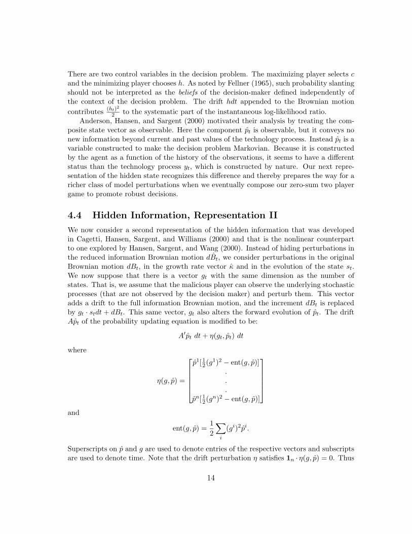
4.4 Hidden Information, Representation II

We now consider a second representation of the hidden information that was developedin Cagetti, Hansen, Sargent, and Williams (2000) and that is the nonlinear counterpartto one explored by Hansen, Sargent, and Wang (2000). Instead of hiding perturbations inthe reduced information Brownian motion dBt, we consider perturbations in the originalBrownian motion dBt, in the growth rate vector κ and in the evolution of the state st.We now suppose that there is a vector gt with the same dimension as the number ofstates. That is, we assume that the malicious player can observe the underlying stochasticprocesses (that are not observed by the decision maker) and perturb them. This vectoradds a drift to the full information Brownian motion, and the increment dBt is replacedby gt · stdt + dBt. This same vector, gt also alters the forward evolution of pt. The driftApt of the probability updating equation is modified to be:

A′pt dt + η(gt, pt) dt

where

η(g, p) =

p1[12(g1)2 − ent(g, p)]

.

.

.pn[12(gn)2 − ent(g, p)]

and

ent(g, p) =12

∑i

(gi)2pi.

Superscripts on p and g are used to denote entries of the respective vectors and subscriptsare used to denote time. Note that the drift perturbation η satisfies 1n · η(g, p) = 0. Thus

14

Game dB distortion dB distortion A′p distortion κ distortion

Hidden I dB + h dt κ + σyh1n

Hidden II dB + g · s dt dB + g · p dt A′p + η(g, p) κ + σyg

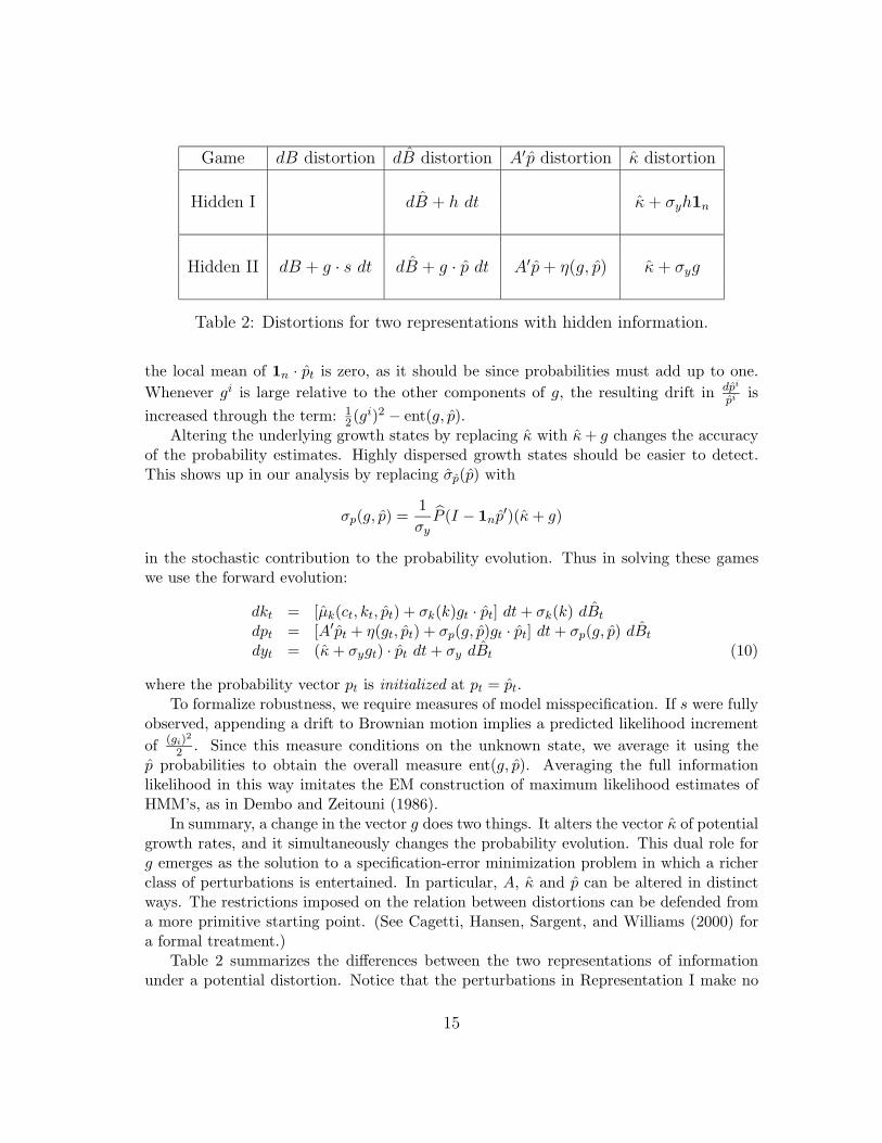
Table 2: Distortions for two representations with hidden information.

the local mean of 1n · pt is zero, as it should be since probabilities must add up to one.Whenever gi is large relative to the other components of g, the resulting drift in dpi

pi isincreased through the term: 1

2(gi)2 − ent(g, p).Altering the underlying growth states by replacing κ with κ + g changes the accuracy

of the probability estimates. Highly dispersed growth states should be easier to detect.This shows up in our analysis by replacing σp(p) with

σp(g, p) =1σy

P (I − 1np′)(κ + g)

in the stochastic contribution to the probability evolution. Thus in solving these gameswe use the forward evolution:

dkt = [µk(ct, kt, pt) + σk(k)gt · pt] dt + σk(k) dBt

dpt = [A′pt + η(gt, pt) + σp(g, p)gt · pt] dt + σp(g, p) dBt

dyt = (κ + σygt) · pt dt + σy dBt (10)

where the probability vector pt is initialized at pt = pt.To formalize robustness, we require measures of model misspecification. If s were fully

observed, appending a drift to Brownian motion implies a predicted likelihood incrementof (gi)

2

2 . Since this measure conditions on the unknown state, we average it using thep probabilities to obtain the overall measure ent(g, p). Averaging the full informationlikelihood in this way imitates the EM construction of maximum likelihood estimates ofHMM’s, as in Dembo and Zeitouni (1986).

In summary, a change in the vector g does two things. It alters the vector κ of potentialgrowth rates, and it simultaneously changes the probability evolution. This dual role forg emerges as the solution to a specification-error minimization problem in which a richerclass of perturbations is entertained. In particular, A, κ and p can be altered in distinctways. The restrictions imposed on the relation between distortions can be defended froma more primitive starting point. (See Cagetti, Hansen, Sargent, and Williams (2000) fora formal treatment.)

Table 2 summarizes the differences between the two representations of informationunder a potential distortion. Notice that the perturbations in Representation I make no

15

explicit reference to the evolution of the hidden state s. A drift distortion h dt (inde-pendent of s) is appended to the Brownian motion increment for the Brownian motionassociated with investors’ information. In contrast, the counterpart to h, denoted by g,in Representation II can depend on states and hence can capture changes in the hiddengrowth rates.

We will subsequently define two HMM games associated with the two representationsof information. These games are designed to deliver forms of robustness by having afictitious agent choose perturbations in a malevolent way. Thus the decision variablefor this fictitious agent is h for HMM Game I and g for HMM Game II. We limit themalevolence by adding quadratic penalties to the objectives of decision-makers scaledby θ. We use the statistical discrepancy measures described earlier as penalties. Thesepenalties are h2

2 for Game I and∑

i(gi)

2

2 for Game II. The resulting two-player games,described later in equation (12), will be Markov, which gives computationally tractablealternatives to the Markov decision problem without robustness.

4.5 A Full Information Benchmark

For comparisons, we will also consider a model in which st is directly observed. Like HiddenInformation Game I, this game is formulated as in Anderson, Hansen, and Sargent (2000),except with a different vector of state variables. The actual state s replaces vector p ofstate probabilities. We use p to form a time series for s by assigning s to the low growthstate when p exceeds one half and to the high growth state when p is greater than onehalf.

5 Value Functions

We have described representations of information for a HMM model and another full in-formation benchmark. We now use these representations of information to solve resourceallocation problems that incorporate a concern about robustness. These model specifi-cation games are all Markov and have a single value function. In this section we reportthe partial differential equations for these functions, which are known as Hamilton-Jacobi-Bellman (HJB) equations. To study these games, we will solve these differential equationsnumerically as described in Appendix C.

5.1 Preferences and Discounting

It is convenient to scale consumption and capital by the technology level. This will even-tually allow us to derive HJB equations that do not depend on y, but only on (k, p), thussimplifying our numerical analysis. This scaling, however, has the effect of introducingstochastic discounting into the preferences. We will use this same discounting to evaluatemodel misspecification.

16

Let U(C) be the instantaneous flow of utility, which we parameterize using a constantelasticity of substitution. The time t contribution to the discounted power utility functionis:

exp(−ρt)U(Ct) = exp(−ρt)(Ct)1−γ/(1 − γ)= exp[(1 − γ)yt − ρt] (ct)1−γ/(1 − γ)

= Y ∗t

(ct)1−γ

1 − γ

where ρ is the subjective rate of discount and

Y ∗t ≡ exp[(1 − γ)yt − ρt].

We now view Y ∗t as a stochastic discount factor, and c = C

Y as a decision variable. Noticethat

dY ∗t = Y ∗

t

((1 − γ) dyt +

[(1 − γ)2(σy)2

2− ρ

]dt

). (11)

In the robustness games, Y ∗t is used to discount instantaneous utilities and discrepancy

measures.

5.2 Hamilton-Jacobi-Bellman Equations

Let x be a composite state vector that includes (k, p, Y ∗). The stochastic evolution (9)and (11) for Game I can be written as:

dxt = µ1x(ct, ht, xt)dt + σ1

x(xt)dBt

where ht is a scalar perturbation and σ1x is a column vector. This column vector depends

on x, but not on h. As explained in appendix B, the HJB equation for Game I is:

0 = maxc

minh

Y ∗[

c1−γ

1 − γ+ θ

h2

2

]+ µ1

x(c, h, x)′ · ∇W 1(x) +12[σ1

x(x)]′∂2W 1(x)∂x∂x′ [σ1

x(x)].

(12)

where ∇ is the gradient. The HJB equation is composed of two parts, one representingthe contribution of the current reward to the value function, the other representing theexpected change in the value function W 1. The first part is

Y ∗[

c1−γ

1 − γ+ θ

h2

2

]which contains the current utility of the decision maker, plus, as explained in previoussection, a penalization for the malicious player. As discussed, the penalization givenby the entropy measure of the discrepancy between the approximating and perturbed

17

models. Note that the entropy term h2

2 is multiplied by a (positive) parameter θ, thatcontrols the degree of robustness that is sought. When θ is ∞, the penalization is also ∞,and therefore no perturbations are allowed. Therefore, θ = +∞ gives the usual resourceallocation problem without robustness. Smaller of θ result in smaller penalization andhence accommodate a larger exploration of alternative models. The calibration of θ in oursimulation is described in section 7.

For Game II we replace (9) with (10). We write the stochastic evolution as:

dxt = µ2x(ct, gt, xt)dt + σ2

x(gt, xt)dBt

where gt is an n-dimensional perturbation and σ2x(gt, xt) is a column vector. In contrast

to Game I, this volatility vector depends on the perturbation g. The HJB equation is ofthe same form as Game I, but with a different stochastic evolution:

0 = maxc

ming

Y ∗[c1−γ

1 − γ+

θ

2

∑i

(gi)2pi] + µ2x(c, g, x) · ∇W 2(x)

+12[σ2

x(g, x)]′∂2W 2(x)∂x∂x′ [σ2

x(g, x)]. (13)

Under Game II, the local mean of the value function W 2 is the negative of

Y ∗[

c1−γ

1 − γ+

θ

2

∑i

(gi)2pi

]appropriately optimized. We again nest a decision problem without concern for robustnessby setting the tuning parameter θ to infinity.

5.3 Computations

We compute the value functions for these games numerically. Given the presumed struc-ture of shocks, we thought it best to avoid using the linearization techniques commonlyemployed in macroeconomics. Conveniently, the value functions are linear in the stochas-tic discount factor. That is, they satisfy W (k, p, Y ∗) = Y ∗V (k, p), and as a consequencewe can focus our computations on determining V . This scaling property follows becausedifferential equations (12) and (13) are both linear in Y ∗.

For both games, consumption satisfies:

c∗ =[∂V

∂k(k, p)

]− 1γ

. (14)

Moreover, objective (12) is quadratic in the scalar h and (13) is quadratic in the vector g.Thus for given value functions, the control laws for c, g and h are easy to compute. Thesolution algorithm in Appendix C exploits this simplicity.

We solve the complete information game in an entirely analogous fashion, except inthis case we eliminate the dependence on p and carry along a vector of value functions(one for each growth state) that only depend on k.

18

6 An Illustrative Growth Economy

As we have seen, the HMM version of the stochastic growth model separates as follows.We can first solve a signal extraction problem and deduce the hidden state probabilities.We can then use these hidden state probabilities in conjunction with the directly observedtechnology shock process as a multivariate stochastic forcing process for a robust resourceallocation problem. In this section we take the time paths for the technology process andthe hidden state probabilities as inputs into our calculations. These are the exogenousforcing processes for our models. The robust resource allocation problems imply trajecto-ries for capital, consumption and investment. We now study these quantity implicationsto understand better the precautionary motive induced by robustness.

6.1 Implications for Capital Accumulation

To illustrate the impact of robustness, we compute the implied time series for k andcompare them to actual data. To make this comparison, we must fully parameterizepreferences. Initially we set the power utility parameter γ = 2, subjective discount rateρ = .04 and depreciation rate δ = .07. We initialize the initial capital to technology ratioto the corresponding level in the data in 1959:Q1, and then compute the solution for thevarious decision problems by using the trajectories of y and p shown in Figure 1.

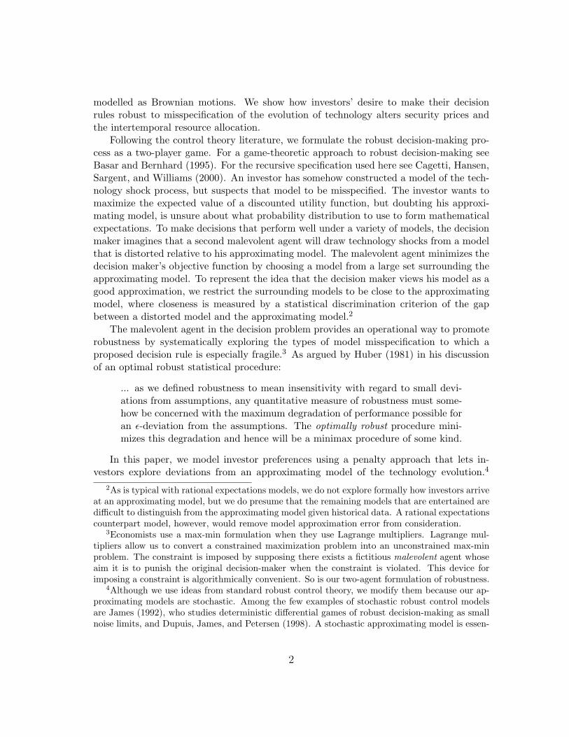
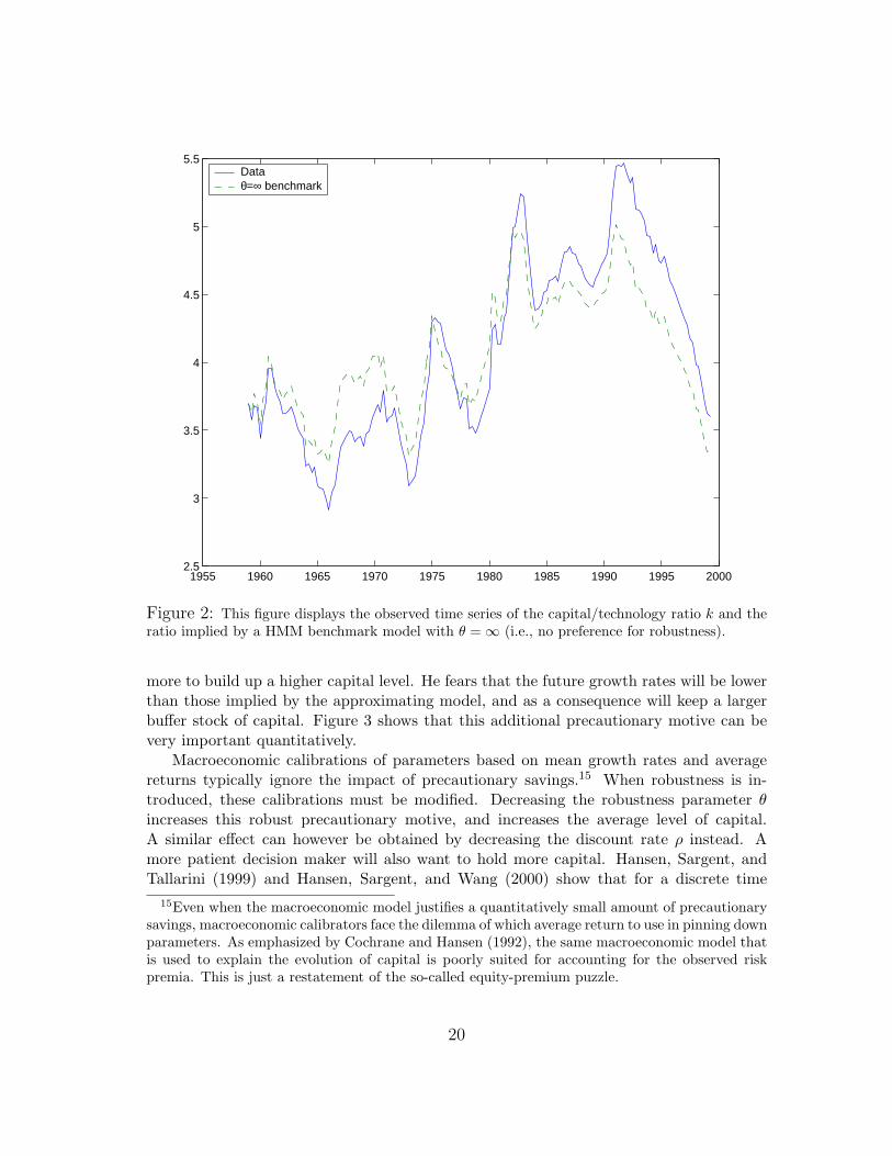
Figure 2 shows the evolution of our endogenous state variable k, which can be inter-preted as the capital/effective labor ratio. The figure reports the evolution of k for thedata and for the hidden information decision problem without robustness (θ = ∞). Thetime path for k implied by the θ = ∞ model mimics the actual data, although the modelgenerates a higher trajectory early on and a lower one later. The overall similarity to thedata should come as no surprise since the parameter configurations were selected in partto match the growth features of the model.13

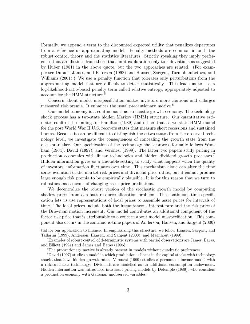
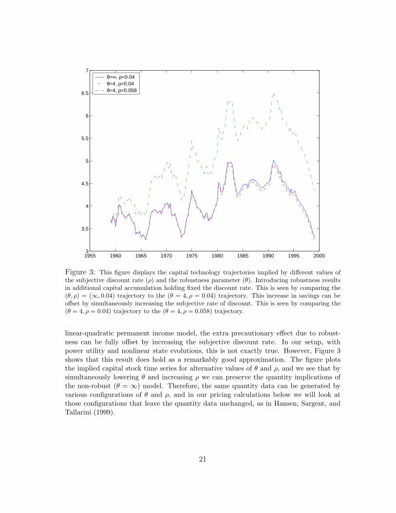
The effect of robustness on the evolution of k is depicted in Figure 3. The figure showsthat the robustness games imply a higher level of capital than the corresponding non-robust decision problems. After starting with the same initial capital, a decision-makerendowed with a concern about model misspecification builds up the capital stock morequickly. Robustness acts as an additional precautionary motive for saving, and generatesa higher buffer stock of capital.

In the standard expected utility framework, precautionary savings are generated bythe possibility of bad shocks coming from a given and pre specified probability distribu-tion. These effects are known to be small when calibrated to macroeconomic measuresof uncertainty.14 In our robust setup, the decision-maker considers also the potentialmisspecification of his approximating model. This induces an additional precautionarymechanism that may not be quantitatively small. The robust social planner will save

13Moreover, the technology process was itself extracted from aggregate quantity data.14See Aiyagari (1994) and Krusell and Smith (1998) among others for a discussion of this issue.

Small precautionary savings is needed to justify the long-standing tradition of macroeconomiccalibrations to steady-state relations.

19

1955 1960 1965 1970 1975 1980 1985 1990 1995 20002.5

3

3.5

4

4.5

5

5.5Data θ=∞ benchmark

Figure 2: This figure displays the observed time series of the capital/technology ratio k and theratio implied by a HMM benchmark model with θ = ∞ (i.e., no preference for robustness).

more to build up a higher capital level. He fears that the future growth rates will be lowerthan those implied by the approximating model, and as a consequence will keep a largerbuffer stock of capital. Figure 3 shows that this additional precautionary motive can bevery important quantitatively.

Macroeconomic calibrations of parameters based on mean growth rates and averagereturns typically ignore the impact of precautionary savings.15 When robustness is in-troduced, these calibrations must be modified. Decreasing the robustness parameter θincreases this robust precautionary motive, and increases the average level of capital.A similar effect can however be obtained by decreasing the discount rate ρ instead. Amore patient decision maker will also want to hold more capital. Hansen, Sargent, andTallarini (1999) and Hansen, Sargent, and Wang (2000) show that for a discrete time

15Even when the macroeconomic model justifies a quantitatively small amount of precautionarysavings, macroeconomic calibrators face the dilemma of which average return to use in pinning downparameters. As emphasized by Cochrane and Hansen (1992), the same macroeconomic model thatis used to explain the evolution of capital is poorly suited for accounting for the observed riskpremia. This is just a restatement of the so-called equity-premium puzzle.

20

1955 1960 1965 1970 1975 1980 1985 1990 1995 20003

3.5

4

4.5

5

5.5

6

6.5

7θ=∞, ρ=0.04θ=4, ρ=0.04 θ=4, ρ=0.058

Figure 3: This figure displays the capital technology trajectories implied by different values ofthe subjective discount rate (ρ) and the robustness parameter (θ). Introducing robustness resultsin additional capital accumulation holding fixed the discount rate. This is seen by comparing the(θ, ρ) = (∞, 0.04) trajectory to the (θ = 4, ρ = 0.04) trajectory. This increase in savings can beoffset by simultaneously increasing the subjective rate of discount. This is seen by comparing the(θ = 4, ρ = 0.04) trajectory to the (θ = 4, ρ = 0.058) trajectory.

linear-quadratic permanent income model, the extra precautionary effect due to robust-ness can be fully offset by increasing the subjective discount rate. In our setup, withpower utility and nonlinear state evolutions, this is not exactly true. However, Figure 3shows that this result does hold as a remarkably good approximation. The figure plotsthe implied capital stock time series for alternative values of θ and ρ, and we see that bysimultaneously lowering θ and increasing ρ we can preserve the quantity implications ofthe non-robust (θ = ∞) model. Therefore, the same quantity data can be generated byvarious configurations of θ and ρ, and in our pricing calculations below we will look atthose configurations that leave the quantity data unchanged, as in Hansen, Sargent, andTallarini (1999).

21

6.2 Other Quantity Implications

The approximating model fails to capture some aspects of the data. In addition to ab-stracting from labor supply, the model is known to imply too much consumption volatility.The ratio of the standard deviation in consumption growth to that in output is approxi-mately one in our model, but only one half in the data. The excess consumption volatilityimplied by the model suggests that the risk premia are likely to be larger than in a modelwith more plausible consumption variability. However, as we will see in section 8 theyare still substantially lower than in the data, and this increased consumption variabilitycannot, per se, explain the observed risk premia. The aim of our exercises is to take asimple, widely used and pedagogically valuable model, and study how a concern aboutrobustness alters what is typically viewed as risk premia by a financial econometrician.Adding various elements to the approximating model (such as a richer dynamic for thetechnological process, various types of adjustment costs and intertemporal complementar-ities in preferences) may generate more realistic consumption variabilities, but will alsointroduce make the model more difficult to solve and arguable distract us from our pri-mary interest. We have chosen to use a simpler model to emphasize how a concern aboutmodel misspecification can alter security market prices.

7 Tuning Robustness

The parameter θ is used to govern the extent of robustness in HMM Games I and IIand in the full information counterpart. It is difficult to restrict the parameter θ a prioriindependent of the approximating model and of the rules of the game. In this section wedescribe a different approach that follows an idea in Anderson, Hansen, and Sargent (2000).We explore families of robustness games indexed by θ. We not presume that θ for onegame has the same meaning as for another, and the θ’s used in our calculations will differacross games. Associated with each θ (and each game) is an implied alternative worst-casemodel used to enforce robustness in decision-making. This alternative model is obtained aspart of the solution to a two-player game. Moreover, there is a corresponding conditionalrelative entropy process that measures the discrepancy between the approximating modelthe alternative worst-case model. A smaller value of θ reduces the penalty for exploringmodel misspecification. Typically, this results in a larger entropy process associated withthe worst-case model.

Comparing the entropy processes across games is more informative than comparingdirectly the values of θ. As we have noted previously, the discrepancy measures we useare information-based measures related closely to log-likelihood ratios. A larger entropyprocess implies that it is easier for a statistician to discriminate between the approximat-ing model and the worst-case model given historical data. While rational expectationspresumes there is no discrepancy (θ = ∞), we wish to allow for the possibility of modelmisspecification that is small in a statistical sense. We operationalize this by choosing θto limit the entropy process that comes from the Markov game solution to be small.

22

Given a time series of y, we could compute the log-likelihood ratio to test one model(the approximating model h = 0) versus the alternative misspecified one (h = h∗). Asexplained in section 4.2, the entropy term (h∗)2

2 represents the conditional expectation of

the instantaneous contribution to the log-likelihood ratio. Cumulating the process { (h∗t )2

2 }over an interval gives the predictable component to the log-likelihood over that sameinterval.16 To simplify comparisons across games, we will hold fixed the cumulation overthe observed sample. In our computations, we set this to .6, which is arbitrary but givesus a useful benchmark for making comparisons across games.

For HMM Game II, matters are more complicated because of the hidden Markov state.Our measure of discrepancy is based on an averaging conditional entropy over the hiddenstates: 1

2

∑i(gi)2pi. An analogous approach is used in likelihood estimation based on the

EM algorithm. This algorithm is commonly used because of its computational convenienceand its relation to likelihood ratios. Thus the discrepancy measure is distinct, but closelyrelated to, a conditional expectation of a log-likelihood ratio.

Anderson, Hansen, and Sargent (2000) and Hansen, Sargent, and Wang (2000) providemore sophisticated discussions linking statistical detection to the choice of θ. Considerthe following simplified problem of statistical discrimination. Use historical data to makea pairwise choice between an approximating model and a worst-case model. This can beformulated as a Bayesian decision problem. Two types of errors are possible dependingupon which model is correct. The resulting detection-error probabilities provide a formalway to quantify statistical discrimination as originally suggested by Chernoff (1952). LikeChernoff, Anderson, Hansen, and Sargent (2000) use bounds on detection error probabil-ities between competing models to help understand better any particular value of θ. Forinstance, a large value of θ is one for which the worst case model is hard to detect statisti-cally given the approximating model and conversely. Similar to the rational expectationsintuition, the misspecified models to which a decision-maker aims to be protected againstare those that could not have been ascertained easily given historical data.

At least in the case of diffusions, conditional entropy is an important input into thesebounds on detection error probabilities. Instead of using bounds, Hansen, Sargent, andWang (2000) compute detection error probabilities via simulation and allow for hiddenMarkov states. Computations such as these are more refined ways to use the Bayesiantheory of statistical discrimination to assist in the choice of θ. Here we use a less ambitiousapproach of fixing the sample accumulation of the relative entropy process. When relativeentropy is constant, we may compute easily a Chernoff-type bound on the detection-errorprobabilities in terms of the entropy accumulation, however. For an entropy accumulationof .6, the upper bound on the detection-error probability is .43.17 Thus if forced to

16This reference to a predictable component is ambiguous without stating which model is used. Itturns out that under either the approximating model or the worst-case model, this same expressionis valid. Expectations of functions of this cumulation would differ depending upon which modelwas used in the computation, however. The symmetry in the instantaneuos contributions does nothold in a full information game with observable jump components.

17The probability of making a classification error is bounded above by 12 exp(− 1

4ce) where ce is

23

Game θ ρHidden I 4.0 .058Hidden II 6.5 .046

Full Information 4.4 .055HMM Benchmark ∞ .040

Table 3: This table reports the values of the robustness parameter θ and the subjec-tive discount rate ρ that are used in our subsequent calculations. These configura-tions leave the time path for the capital/technology ratio virtually the same as thatfor the θ = ∞ economy with hidden information. The sample sum of the conditionalentropies are: .60 for HMM Game I, .60 for HMM Game II, and a slightly larger .61for the full information benchmark.

decide between the approximating model and the worst-case model, a statistician shouldexpect mistakes to occur frequently. Unfortunately, as we will see, that assumption ofconstant relative entropy process is counterfactual for our models. Thus our use of .6 forthe entropy accumulation is only a rough way to get comparability across games and isnot meant as a way to give a definitive choice of the parameter θ. In fact, we suspectthat even considerably smaller values of θ might be reasonable for our model economies.Moreover, there are other potential approaches for tuning the robustness parameter θ.While detection error analysis eliminates candidate models that should be easy to uncoverfrom historical data, it considers only a very highly stylized model selection problem. Theutility consequences of being robust and the costs of active learning arguably should alsocome into play.18

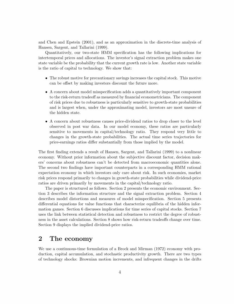
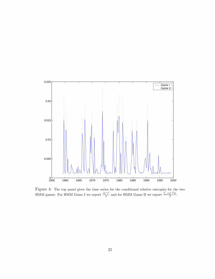
Based on detection-error considerations, we employed the θ and ρ pairs reported inTable 3 in our subsequent calculations. These choices make the cumulation of relative en-tropy remain about the same across games. We report the time series of entropy measuresfor both HMM games in Figure 4. There is considerable variability in these measures,with more variability in the entropy measures for HMM Game II than for Game I. Theentropies for both HMM games are particularly large when the investors are unsure whichgrowth state they are in as measure by p.

the accumulation of the conditional entropy.18We envision that investors confront a much more complicated problem in statistical discrim-

ination, one that would entertain a wide array of models and would use the decision problem toweight the errors in misclassifying models. Implicitly, we are presuming that when confronted withsuch a problem, the investors decide that model discrimination is too difficult and focus insteadon making their investment decisions robust.

24

1955 1960 1965 1970 1975 1980 1985 1990 1995 20000

0.005

0.01

0.015

0.02

0.025Game I Game II

Figure 4: The top panel gives the time series for the conditional relative entropies for the twoHMM games. For HMM Game I we report (h∗)2

2 and for HMM Game II we report∑

i(g∗i )2pi

2 .

25

8 Local Risk and Uncertainty Prices

One common way of studying the dynamic implications of a model is to report the impliedimpulse response functions. Since our model is explicitly nonlinear, impulse-responsefunctions based on linear approximations seem ill-suited to characterize the implicationsof these models. Instead we report plots of prices as functions of the state variables in themodel and the time series implied by the historically observed technology levels.

The HMM formulations imply a particular Markov evolution for the technology shockprocess where the Markov chain state probabilities become an additional state variable.As we showed in Figure 1, a time series of these state probabilities can be constructed fromthe observed data on the technology level. For both HMM games we solve numericallyfor the law of motion for the capital stock. Using this solution and a given time series forthe state probabilities, we recursively generate a time series for the implied capital stock.Thus from a given time series trajectory for the technology shock process, we can computetime series for the state probabilities and the capital stock implied by the model. Thesetime series will be used in some of the calculations that follow.

As we noted above, the effect of robustness on the capital evolution can be offsetby increasing the rate of discount. In the calculations in this subsection we experimentwith different levels of the robustness parameter θ, varying ρ to maintain the quantityimplications. Given that the capital stock trajectory remains essentially the same acrossgames, the instantaneous risk-free rate measured by the marginal product of capital alsoremains the same. The shadow prices of the Brownian motion increments, however, willdiffer.

We study the (local) pricing of dB for our two decision-models in the presence ofhidden information. Consider the local relation between the instantaneous return on asecurity µr, its factor loading on the Brownian increment σr, and the risk free rate µf :

µr − µf = σrλ.

Then λ is the factor risk price and |λ| is the absolute slope of the mean standard deviationfrontier. In our model so far, there is a single Brownian motion factor dB. Anderson,Hansen, and Sargent (2000) and Chen and Epstein (2001) show that the factor price ofthe Brownian increments dB can be decomposed into two prices: the usual price for risk,and a price of model uncertainty.19 Thus the factor price λ is the sum

λ = λm + λu.

The price of risk λm is obtained by applying a formula from Breeden (1979)’s analysis of aconsumption-based asset pricing model. This risk price is given by (minus) the weighting

19Anderson, Hansen, and Sargent (2000) and Chen and Epstein (2001) differ in the way thebeliefs that dictate prices are deduced. The local prices for Game I can be viewed as a specialcase of those in Anderson, Hansen, and Sargent (2000). As we have seen, however, the beliefsthat support the local Game II solution exploit more details of the HMM structure. Thus GameII solution and prices are not special cases of those reported in Anderson, Hansen, and Sargent(2000).

26

coefficient on Bt in the evolution for the process of the log marginal utility of consumption:

π(k, p, y) = log(C−γ)= −γ log c − γy= log Vk(k, p) − γy

where we have used formula (14) for the consumption-technology ratio c. The coefficienton dB is computed as the sum of partial derivatives with respect to y, p and k:

λm = γσy + σykVkk

Vk− (1 − p)p

κ1 − κ2

σy

Vkp

Vk.

In addition to the usual component λm that depends on the marginal utility of con-sumption, there is a second component, related to the worst-case model that emerges inthe solution to the two-player game. It is the worst-case model that used in place of theapproximating that is used for computing shadow prices. Under this worst-case model, S,the price of the asset evolves according to

dS

S= µr dt + σr(dB + h∗ dt)

in Game I (and with p · g∗ instead of h∗ in Game II). That is, it is as if the drift of theprocess were (µr +σrh

∗) dt instead of µr dt. This augmented drift can be used in Breeden(1979), which introduces an additional component to pricing vis-a-vis the approximatingmodel. Making this drift adjustment, we get λu = −h∗ for Game I and λu = −p · g∗ forGame II. (Note that h∗ and p · g∗ will affect the expression for the risk free rate µf , sinceµf is derived from the drift of the marginal utility of consumption.) Anderson, Hansen,and Sargent (2000) formalize these arguments and provide a more complete derivation ofthe factor price decomposition.

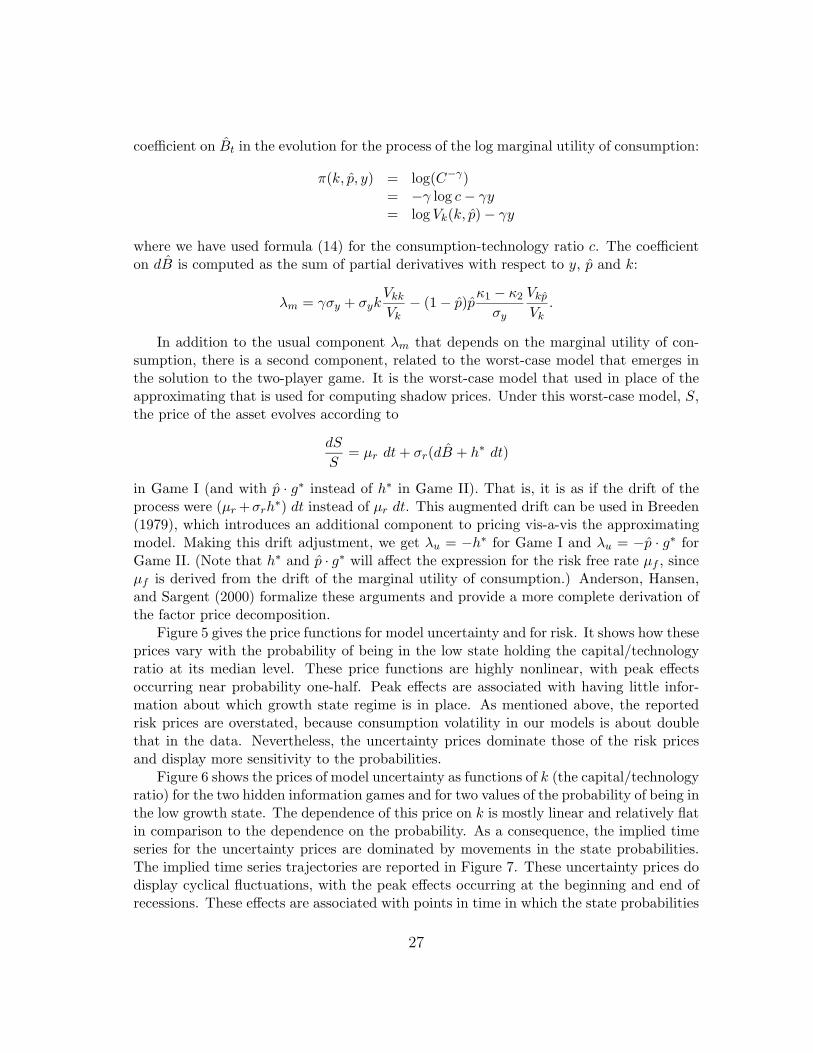
Figure 5 gives the price functions for model uncertainty and for risk. It shows how theseprices vary with the probability of being in the low state holding the capital/technologyratio at its median level. These price functions are highly nonlinear, with peak effectsoccurring near probability one-half. Peak effects are associated with having little infor-mation about which growth state regime is in place. As mentioned above, the reportedrisk prices are overstated, because consumption volatility in our models is about doublethat in the data. Nevertheless, the uncertainty prices dominate those of the risk pricesand display more sensitivity to the probabilities.

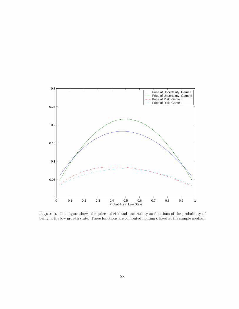
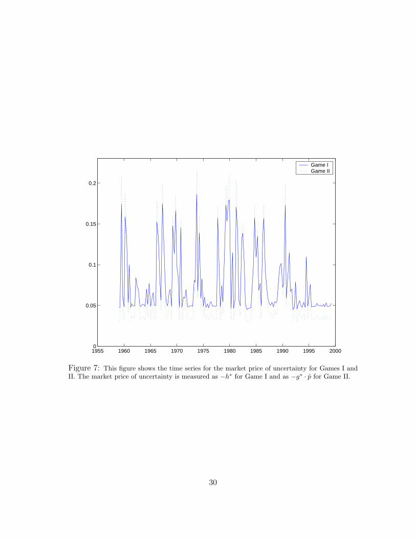
Figure 6 shows the prices of model uncertainty as functions of k (the capital/technologyratio) for the two hidden information games and for two values of the probability of being inthe low growth state. The dependence of this price on k is mostly linear and relatively flatin comparison to the dependence on the probability. As a consequence, the implied timeseries for the uncertainty prices are dominated by movements in the state probabilities.The implied time series trajectories are reported in Figure 7. These uncertainty prices dodisplay cyclical fluctuations, with the peak effects occurring at the beginning and end ofrecessions. These effects are associated with points in time in which the state probabilities

27

0 0.1 0.2 0.3 0.4 0.5 0.6 0.7 0.8 0.9 10

0.05

0.1

0.15

0.2

0.25

0.3

Probability in Low State

Price of Uncertainty, Game I Price of Uncertainty, Game IIPrice of Risk, Game I Price of Risk, Game II

Figure 5: This figure shows the prices of risk and uncertainty as functions of the probability ofbeing in the low growth state. These functions are computed holding k fixed at the sample median.

28

2 2.5 3 3.5 4 4.5 5 5.5 6 6.5 70

0.05

0.1

0.15

0.2

0.25

0.3

Capital

Game I, p=0.05 Game II, p=0.05Game I, p=0.5 Game II, p=0.5

Figure 6: This figure shows the market price of uncertainty as a function of k for Games I andII and for two different values of the probability of being in a low growth state.

are each about a half. The prices are lower in Game I than Game II for probabilities nearone half but higher for probabilities close to zero or one. (See also Figure 5.) Thus themodel produces substantial cyclical fluctuations in what financial econometricians mightmistakenly call risk premia. The high market prices of uncertainty occur not because ofconfidence in low growth but rather because of ambiguity about which growth regime iscurrently in play.

9 Price-Earnings Ratios

To study price-earnings ratios, we apply the HMM model simultaneously to the technol-ogy shock process and an earnings process. Growth rates in the technology and earningsrespond to the same two-state hidden Markov chain. For the purposes of pricing, wetreat the earnings process as a stream of dividends: claims to consumption to be priced.These dividends are not an extra source of consumption, but merely a specification ofan intertemporal payoff stream to be priced. Production takes place as before, but the

29

1955 1960 1965 1970 1975 1980 1985 1990 1995 20000

0.05

0.1

0.15

0.2

Game I Game II

Figure 7: This figure shows the time series for the market price of uncertainty for Games I andII. The market price of uncertainty is measured as −h∗ for Game I and as −g∗ · p for Game II.

30

1955 1960 1965 1970 1975 1980 1985 1990 1995 20000.8

1

1.2

1.4

1.6

1.8

2

2.2

2.4

2.6

2.8Log Real Earnings (Left Axis) Log Technology Shock (Right Axis)

1955 1960 1965 1970 1975 1980 1985 1990 1995 2000−4.8

−4.66

−4.52

−4.38

−4.24

−4.1

−3.96

−3.82

−3.68

−3.54

−3.4

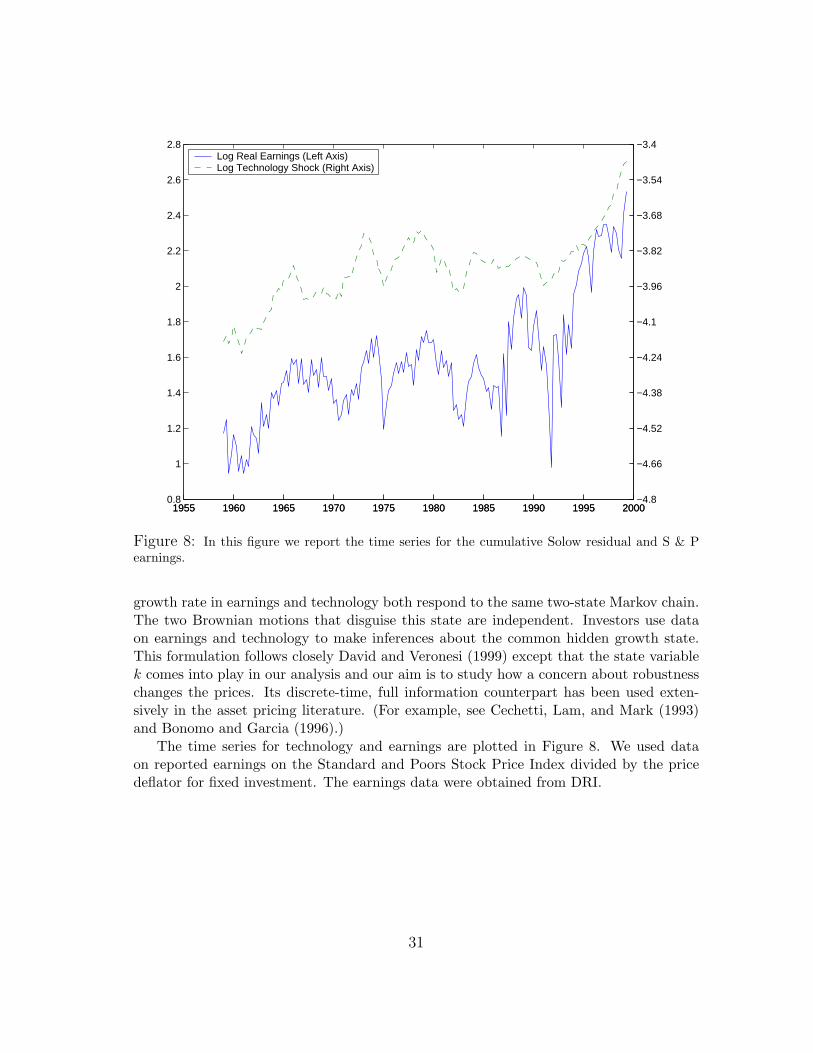
Figure 8: In this figure we report the time series for the cumulative Solow residual and S & Pearnings.

growth rate in earnings and technology both respond to the same two-state Markov chain.The two Brownian motions that disguise this state are independent. Investors use dataon earnings and technology to make inferences about the common hidden growth state.This formulation follows closely David and Veronesi (1999) except that the state variablek comes into play in our analysis and our aim is to study how a concern about robustnesschanges the prices. Its discrete-time, full information counterpart has been used exten-sively in the asset pricing literature. (For example, see Cechetti, Lam, and Mark (1993)and Bonomo and Garcia (1996).)

The time series for technology and earnings are plotted in Figure 8. We used dataon reported earnings on the Standard and Poors Stock Price Index divided by the pricedeflator for fixed investment. The earnings data were obtained from DRI.

31

9.1 Earnings Evolution

In our robust resource allocation problems we used the following model for log technologyand log earnings: [

dyt

det

]=

[κ11 κ12

κ21 κ22

]stdt +

[σy 00 σe

]dBt

where dBt is now a two-dimensional Brownian motion. We used the parameter valuesreported in Table 4. These parameters were obtained by estimating a discrete-time coun-terpart HMM model using an EM algorithm. While we used a two-state specification tocompute prices, we were actually compelled to fit a more complicated model to capturethe seasonality in the earnings data.20 The estimates of the parameters that govern thetechnology evolution were very close to those obtained when we estimated the HMM modelusing only the technology data. In our calculations we used the same parameters for thetechnology evolution for both models. (Compare Table 1 to Table 4). Since the standarddeviation for the earnings process is substantially higher than that for technology, theimplied state probability estimates for the technology-earnings model are very close tothose reported in Figure 1. The technology process is the primary source of informationabout the hidden growth state.

9.2 Price calculation

To compute the price function for the HMM games, we use the familiar implication thatthe local mean of the marginal-utility scaled price should be minus the marginal-utilityscaled dividend. The solutions to the respective robustness games provide us with theformula of the local mean of the marginal-utility scaled dividends.

To formalize this idea, we form a state vector z that contains (k, p, Y ∗, e). Let µ1z denote

the drift implied by the Markov solution to HMM Game I and Σ1z the corresponding

diffusion matrix for the bivariate Brownian motion dBt associated with the investors’information set. The drift vector µ1

z includes terms which reflect how the worst-caseperturbations h∗ affect the state variables and hence adjusts for model uncertainty. Thisis consistent with our incremental pricing results above. Let Π1 denote the marginal utilityscaled pricing function that maps the composite state z into the marginal utility scaledprice. This function satisfies the partial differential equation:

µ1z · ∇Π1 +

12trace

(Σ1

z

∂2Π1

∂z∂z′

)= − exp(e)(C1)−γY ∗. (15)

20An independent, two-state seasonal Markov chain was introduced in the estimation. Thisseasonal chain only altered the growth rates for earnings. According to our estimates, in oneseasonal state growth is reduced by .0836 and in the other it is enhanced by this same amount.The quarterly transition from reduced growth seasonal state to high seasonal state is essentiallyone while the transition in the other direction is .986. We deliberately avoid the common practiceof using a quarterly series of yearly averages of earnings. While the averaging removes seasonality,it should also change how the signal extraction problem is posed and solved.

32

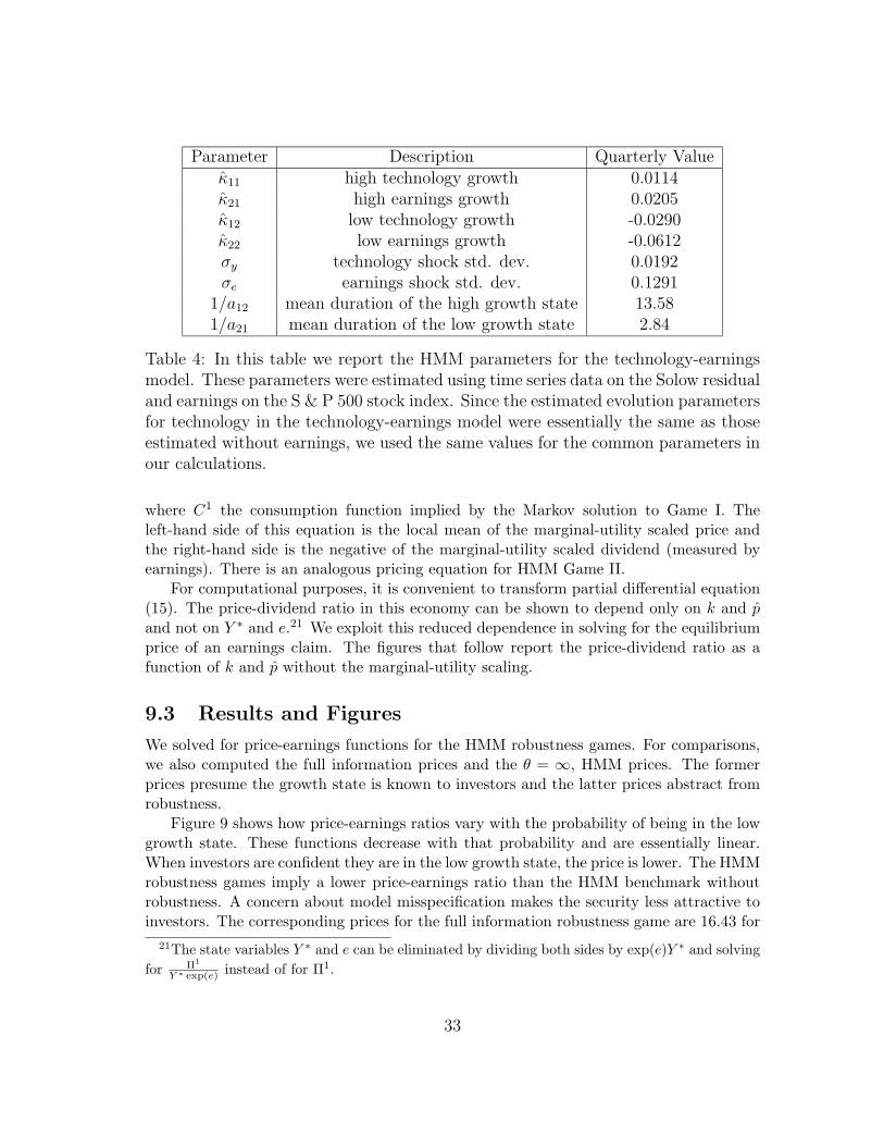
Parameter Description Quarterly Valueκ11 high technology growth 0.0114κ21 high earnings growth 0.0205κ12 low technology growth -0.0290κ22 low earnings growth -0.0612σy technology shock std. dev. 0.0192σe earnings shock std. dev. 0.1291

1/a12 mean duration of the high growth state 13.581/a21 mean duration of the low growth state 2.84

Table 4: In this table we report the HMM parameters for the technology-earningsmodel. These parameters were estimated using time series data on the Solow residualand earnings on the S & P 500 stock index. Since the estimated evolution parametersfor technology in the technology-earnings model were essentially the same as thoseestimated without earnings, we used the same values for the common parameters inour calculations.

where C1 the consumption function implied by the Markov solution to Game I. Theleft-hand side of this equation is the local mean of the marginal-utility scaled price andthe right-hand side is the negative of the marginal-utility scaled dividend (measured byearnings). There is an analogous pricing equation for HMM Game II.

For computational purposes, it is convenient to transform partial differential equation(15). The price-dividend ratio in this economy can be shown to depend only on k and pand not on Y ∗ and e.21 We exploit this reduced dependence in solving for the equilibriumprice of an earnings claim. The figures that follow report the price-dividend ratio as afunction of k and p without the marginal-utility scaling.

9.3 Results and Figures

We solved for price-earnings functions for the HMM robustness games. For comparisons,we also computed the full information prices and the θ = ∞, HMM prices. The formerprices presume the growth state is known to investors and the latter prices abstract fromrobustness.

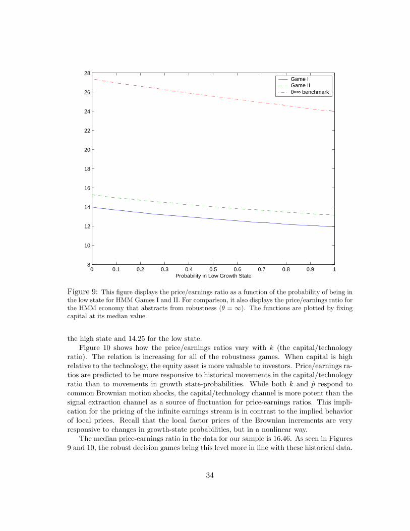
Figure 9 shows how price-earnings ratios vary with the probability of being in the lowgrowth state. These functions decrease with that probability and are essentially linear.When investors are confident they are in the low growth state, the price is lower. The HMMrobustness games imply a lower price-earnings ratio than the HMM benchmark withoutrobustness. A concern about model misspecification makes the security less attractive toinvestors. The corresponding prices for the full information robustness game are 16.43 for

21The state variables Y ∗ and e can be eliminated by dividing both sides by exp(e)Y ∗ and solvingfor Π1

Y ∗ exp(e) instead of for Π1.

33

0 0.1 0.2 0.3 0.4 0.5 0.6 0.7 0.8 0.9 18

10

12

14

16

18

20

22

24

26

28

Probability in Low Growth State

Game I Game II θ=∞ benchmark

Figure 9: This figure displays the price/earnings ratio as a function of the probability of being inthe low state for HMM Games I and II. For comparison, it also displays the price/earnings ratio forthe HMM economy that abstracts from robustness (θ = ∞). The functions are plotted by fixingcapital at its median value.

the high state and 14.25 for the low state.Figure 10 shows how the price/earnings ratios vary with k (the capital/technology

ratio). The relation is increasing for all of the robustness games. When capital is highrelative to the technology, the equity asset is more valuable to investors. Price/earnings ra-tios are predicted to be more responsive to historical movements in the capital/technologyratio than to movements in growth state-probabilities. While both k and p respond tocommon Brownian motion shocks, the capital/technology channel is more potent than thesignal extraction channel as a source of fluctuation for price-earnings ratios. This impli-cation for the pricing of the infinite earnings stream is in contrast to the implied behaviorof local prices. Recall that the local factor prices of the Brownian increments are veryresponsive to changes in growth-state probabilities, but in a nonlinear way.

The median price-earnings ratio in the data for our sample is 16.46. As seen in Figures9 and 10, the robust decision games bring this level more in line with these historical data.

34

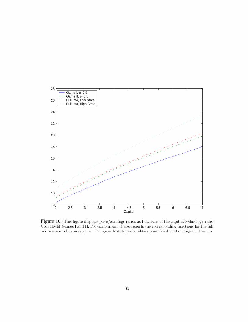
2 2.5 3 3.5 4 4.5 5 5.5 6 6.5 78

10

12

14

16

18

20

22

24

26

28

Capital

Game I, p=0.5 Game II, p=0.5 Full Info, Low State Full Info, High State

Figure 10: This figure displays price/earnings ratios as functions of the capital/technology ratiok for HMM Games I and II. For comparison, it also reports the corresponding functions for the fullinformation robustness game. The growth state probabilities p are fixed at the designated values.

35

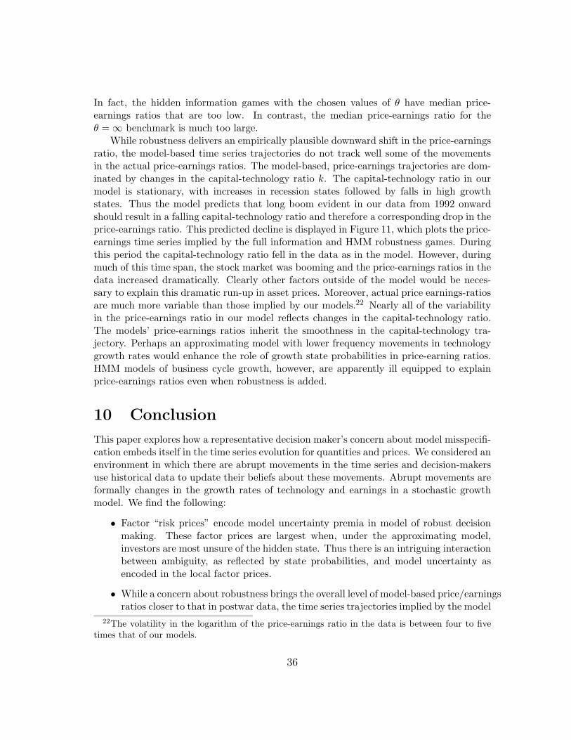
In fact, the hidden information games with the chosen values of θ have median price-earnings ratios that are too low. In contrast, the median price-earnings ratio for theθ = ∞ benchmark is much too large.

While robustness delivers an empirically plausible downward shift in the price-earningsratio, the model-based time series trajectories do not track well some of the movementsin the actual price-earnings ratios. The model-based, price-earnings trajectories are dom-inated by changes in the capital-technology ratio k. The capital-technology ratio in ourmodel is stationary, with increases in recession states followed by falls in high growthstates. Thus the model predicts that long boom evident in our data from 1992 onwardshould result in a falling capital-technology ratio and therefore a corresponding drop in theprice-earnings ratio. This predicted decline is displayed in Figure 11, which plots the price-earnings time series implied by the full information and HMM robustness games. Duringthis period the capital-technology ratio fell in the data as in the model. However, duringmuch of this time span, the stock market was booming and the price-earnings ratios in thedata increased dramatically. Clearly other factors outside of the model would be neces-sary to explain this dramatic run-up in asset prices. Moreover, actual price earnings-ratiosare much more variable than those implied by our models.22 Nearly all of the variabilityin the price-earnings ratio in our model reflects changes in the capital-technology ratio.The models’ price-earnings ratios inherit the smoothness in the capital-technology tra-jectory. Perhaps an approximating model with lower frequency movements in technologygrowth rates would enhance the role of growth state probabilities in price-earning ratios.HMM models of business cycle growth, however, are apparently ill equipped to explainprice-earnings ratios even when robustness is added.

10 Conclusion

This paper explores how a representative decision maker’s concern about model misspecifi-cation embeds itself in the time series evolution for quantities and prices. We considered anenvironment in which there are abrupt movements in the time series and decision-makersuse historical data to update their beliefs about these movements. Abrupt movements areformally changes in the growth rates of technology and earnings in a stochastic growthmodel. We find the following:

• Factor “risk prices” encode model uncertainty premia in model of robust decisionmaking. These factor prices are largest when, under the approximating model,investors are most unsure of the hidden state. Thus there is an intriguing interactionbetween ambiguity, as reflected by state probabilities, and model uncertainty asencoded in the local factor prices.

• While a concern about robustness brings the overall level of model-based price/earningsratios closer to that in postwar data, the time series trajectories implied by the model

22The volatility in the logarithm of the price-earnings ratio in the data is between four to fivetimes that of our models.

36

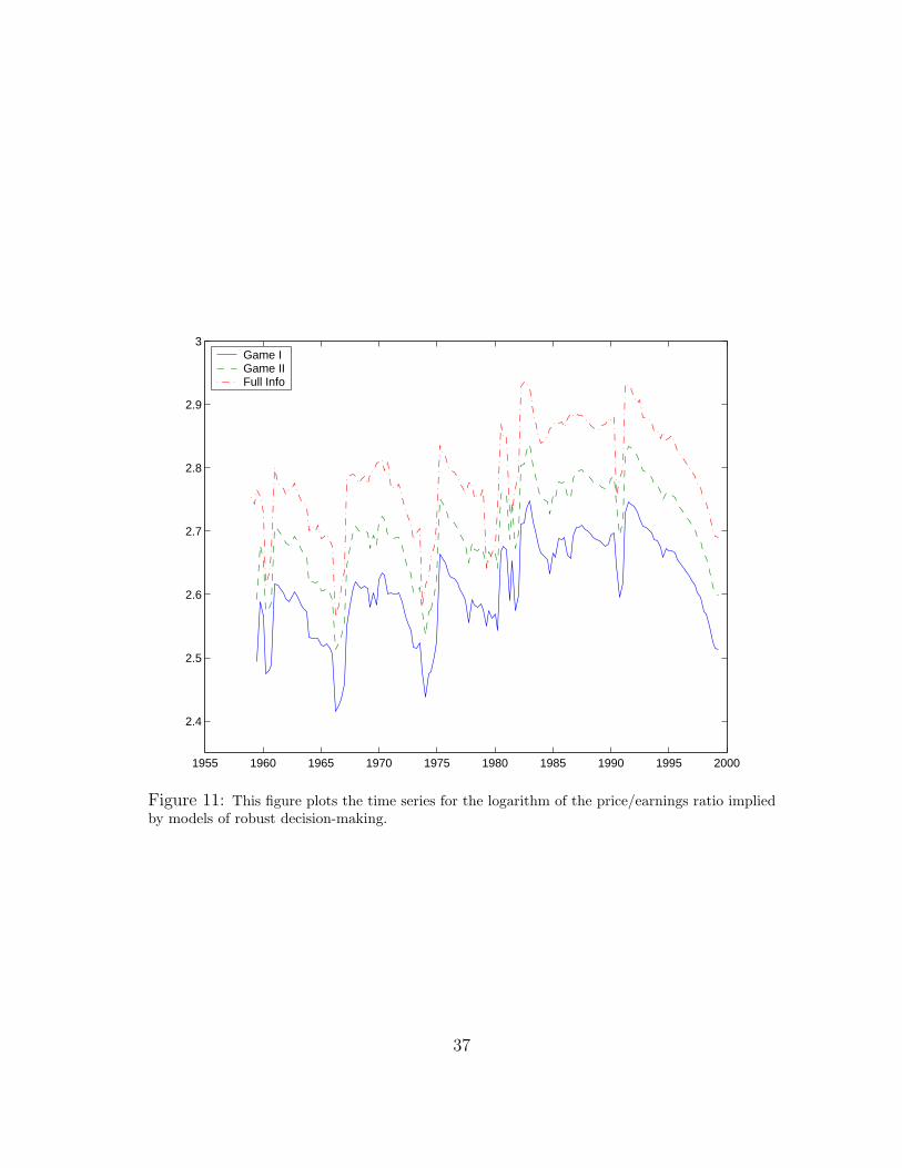
1955 1960 1965 1970 1975 1980 1985 1990 1995 2000

2.4

2.5

2.6

2.7

2.8

2.9

3Game I Game II Full Info

Figure 11: This figure plots the time series for the logarithm of the price/earnings ratio impliedby models of robust decision-making.

37

do not track well the post war data.

We nest an HMM rational expectations model inside our models of investor robustnessby setting θ = ∞. Thus some of conclusions carry over to this rational expectations model.Factor risk prices are predicted to be largest when investors are most unsure of the hiddenstate. Even abstracting from the overall level, the rational expectations model-based price-earnings ratio does not track well that observed in postwar data. The HMM informationstructure we used apparently does little to confront the well known excess volatility insecurity prices.

We have used a stochastic growth model common in macroeconomics and finance. Thisstylized model has been an important benchmark for macroeconomics, and so presents agood laboratory for understanding how a concern about misspecification can alter impli-cations. On the other hand, the stochastic growth model has known empirical deficiencies.Allowing for robustness repairs only some of these shortcomings. Richer transient dynam-ics and possibly multiple sectors and consumers are needed to produce models with betterempirical underpinnings. In particular, a richer learning dynamics may result in quanti-tatively important asymmetries in uncertainty premia in expansions and recessions. Forexample, Chalkley and Lee (1998) and Veldkamp (2000) build models in which businesscycle asymmetries are linked to learning about an unobserved state. The asymmetry isdriven by the interaction between risk aversion and private information in the Chalkleyand Lee (1998) model. A concern about model misspecification could well imitate anenhancement of risk aversion in this environment and amplify the asymmetry betweenrecessions and booms. Veldkamp shows how investors’ decisions to initiate and termi-nate projects create more public information about the hidden state in the economy ingood times than bad times. Introducing this feature into a model like ours could makeuncertainty premia vary more between low growth and high growth regimes.

38

References

Aiyagari, S. R. (1994). Unisured idiosyncratic risk and aggregate savings. QuarterlyJournal of Economcics 104, 219–240.

Anderson, E., L. P. Hansen, and T. Sargent (2000, March). Robustness, detection andthe price of risk. Mimeo.

Basar, T. and P. Bernhard (1995). H∞-Optimal Control and Related Minimax DesignProblems. Boston: Birkhauser.

Baum, L. E. and T. Petrie (1966). Statistical inference for probabilistic functions of afinite state. Annals of Mathematical Statistics 37, 1554–1563.

Boldrin, M., L. Christiano, and J. Fisher (1999). Habit persistence, asset returns andthe business cycle. Mimeo.

Bonomo, M. and R. Garcia (1996). Consumption and equilibrium pricing: An empiricalassessment. Journal of Empirical Finance 3, 239–265.

Breeden, D. (1979). An intertemporal asset pricing model with stochastic consumptionand investment opportunities. Journal of Financial Economics 7, 265–296.

Brock, W. A. and L. J. Mirman (1972, June). Optimal economic growth and uncertainty:The discounted case. Journal of Economic Theory 4 (3), 479–513.

Cagetti, M., L. P. Hansen, T. J. Sargent, and N. Williams (2000). Robust recursiveprediction and control. Mimeo.

Candler, G. V. (1999). Finite difference methods for continuous time dynamic program-ming. In R. Marimon and A. Scott (Eds.), Computational Methods for the Study ofDynamic Economies, pp. 172–194. Oxford: Oxford University Press.

Cecchetti, S. G., P. Lam, and N. C. Mark (1993). The equity premium and the risk-freerate. Journal of Monetary Economics 31, 21–45.

Chalkley, M. and I. H. Lee (1998). Learning and asymmetric business cycles. Review ofEconomic Dynamics 1, 623–645.

Chen, Z. and L. Epstein (2001). Ambiguity, risk and asset returns in continuous time.Forthcoming in Econometrica.

Chernoff, H. (1952). A measure of asymptotic efficiency for tests of a hypothesis basedon the sum of observations. Annals of Mathemtatical Statistics 23, 493–507.

Cochrane, J. and L. P. Hansen (1992). Asset pricing explorations for macroeconomics. InO. J. Blanchard and S. Fischer (Eds.), NBER Macroeconomics Annual, pp. 115–165.Cambridge, MA: The MIT Press.

Cochrane, J. M. (1991, March). Production-based asset pricing and the link betweenstock returns and economic fluctuations. Journal of Finance 46 (1), 209–237.

David, A. (1997, December). Fluctuating confidence in stock markets: Implicationsfor returns and volatility. Journal of Financial and Quantitative Analysis 32 (4),457–462.

39

David, A. and P. Veronesi (1999, November). Option prices with uncertain funda-mentals: Theory and evidence on the dynamics of implied volatilities and over-underreaction in the options market. Mimeo.

Davis, M. H. (1993). Markov Models and Optimization. Chapman & Hall.

Dembo, A. and O. Zeitouni (1986). Parameter estimation of partially observed continu-ous time stochastic processes via the EM algorithm. Stochastic Processes and TheirApplications 23, 91–113.

Detemple, J. (1986). Asset pricing in a production economy with incomplete informa-tion. Journal of Finance 41, 383–390.

Dupuis, P., M. R. James, and I. Petersen (1998). Robust properties of risk sensitivecontrol. LCDS 98-15, Brown University.

Elliott, R. J., L. Aggoun, and J. B. Moore (1995). Hidden Markov Models. Estimationand Control. New York: Springer-Verlag.

Ethier, S. N. and T. G. Kurz (1986). Markov Processes. Characterization and Conver-gence. John Wiley.

Fellner, W. (1965). Probability and Profit: A Study of Economic Behavior AlongBayesian Lines. Irwin Series in Economics. Homewood, Illinois: Richard D. Irwin,Inc.

Hamilton, J. D. (1989, March). A new approach to the economic analysis of nonsta-tionary time series and the business cycle. Econometrica 57 (2), 357–384.

Hamilton, J. D. (1990). Analysis of time series subject to changes in regime. Journal ofEconometrics 45, 39–70.

Hansen, L. P. and R. Jagannathan (1991). Implications of security market data formodels of dynamic economies. Journal of Political Economy 99, 225–262.

Hansen, L. P., T. Sargent, and T. Tallarini (1999, January). Robust permanent incomeand pricing. Mimeo.

Hansen, L. P., T. J. Sargent, G. A. Turmuhambetova, and N. Williams (2001). Robust-ness and uncertainty aversion. Mimeo.

Hansen, L. P., T. J. Sargent, and N. E. Wang (2000). Robust permanent income andpricing with filtering. Macroeconomic Dynamics. forthcoming.

Hansen, L. P. and K. J. Singleton (1983, April). Stochastic consumption, risk aversion,and the temporal behavior of asset returns. Journal of Political Economy 91 (2),249–265.

Huber, P. J. (1981). Robust Statistics. Wiley Series in Probability and MathematicalStatistics. New York: John Wiley and Sons.

James, M. R. (1992). Asymptotic analysis of nonlinear stochastic risk sensitive controland differential games. Mathematics of Control, Signals, and Systems 5, 401–417.

40

James, M. R. and J. Baras (1996). Partially observed differential games, infinite dimen-sional Hamilton-Jacobi-Isaacs equations, and nonlinear H∞ control. SIAM Journalon Control and Optimization 34 (4), 1342–1364.

James, M. R., J. Baras, and R. J. Elliott (1994, April). Risk-sensitive control anddynamic games for partially observed discrete-time nonlinear systems. IEEE Trans-actions on Automatic Control 39 (4), 780–791.

Krusell, P. and A. A. Smith (1998). Income and wealth heterogeneity. Journal of Polit-ical Economy 106, 867–896.

Liptser, R. S. and A. N. Shiryayev (1977). Statistics of Random Processes. New York:Springer-Verlag.

Maenhout, P. J. (1999). Robust portfolio rules and asset pricing. Mimeo.

Merton, R. C. (1975, July). An asymptotic theory of growth under uncertainty. Reviewof Economic Studies 42 (3), 375–393.

Rouwenhorst, K. G. (1995). Asset pricing implications of equilibrium business cyclemodels. In T. F. Cooley (Ed.), Frontiers of Business Cycle Theory, pp. 294–330.Princeton University Press.

Sclove, S. L. (1983, February). Time-series segmentation: A model and a method.Information Sciences 29 (1), 7–25.

Stock, J. and M. Watson (1999). Business cycle fluctuations in US macroeconomic timeseries. In J. Taylor and M. Woodford (Eds.), Handbook of Macroeconomics. Elsevier.Forthcoming.

Veldkamp, L. L. (2000). Slow boom, big crash. manuscript.

Veronesi, P. (1999). Stock market overreaction to bad news in good times: A rationalexpectations equilibrium model. Review of Financial Studies 12, 976–1007.

Veronesi, P. (2000). How does information quality affect stock returns? Journal ofFinance 55, 807–837.

Watson, M. W. (1993, December). Measures of fit for calibrated models. Journal ofPolitical Economy 101 (6), 1011–1041.

Wonham, W. J. (1964). Some applications of stochastic differential equations to optimalnonlinear filtering. SIAM Journal on Control 2 (3), 347–368.

A Generators

To represent the robustness games, we will make use of the generator of Markov processes. It istherefore useful to define it here briefly.23 In our applications the Markov state contains either(k, s, Y ∗), in the full information benchmark, or (k, p, Y ∗), in the hidden information case.

23For a rigorous treatment, see Ethier and Kurz (1986).

41

A Markov process can be specified in terms of the transition probabilities. Associated witheach transition interval is a conditional expectation operator. The family of such operators is aFeller semigroup. The time derivative of the semigroup at the zero interval gives the generatorof the semigroup. The generator captures the local evolution of the process. Since the family(semigroup) of conditional expectation operators can be built from the generator, we may modela Markov process by specifying its generator.

A.1 Full information

In the full information case, the state space is X = R+ × S × R+, where R is the real line, R+ =(0,+∞) and S is the collection of coordinate vectors in Rn. Consider a function f mapping thisstate space into the real line R. This function can be thought of equivalently as a φ : R+×R+ → Rn,where each coordinate function of φ is matched to a state s. If we begin with a function f(k, s, Y ∗)we may form

φ(k, Y ∗) =−−−−−−−→f(k, s, Y ∗)

The~ operation stacks f(k, s, Y ∗) for the n values of s.To construct a Feller semigroup of conditional expectation operators we consider the space of

functions that are continuous on the one-point compactification of the state space X. The collectionof the restrictions of these functions to X is denoted by C. The conditional expectation operatorfor interval τ can be represented as:

Tτf(k, s, Y ∗) = E[f(kτ , sτ , Y ∗τ )|k0 = k, s0 = s, Y ∗ = Y ∗

0 ]

for any τ ≥ 0 and for any f in C. The generator of the semigroup is the time derivative computedusing the metric induced by the sup norm in (k, Y ∗):

Gf = limτ↓0

Tτf − f

τ

for each of the n values of s.The generator is composed by two parts, one relative to the diffusion process for k and Y ∗, and

one relative to the jump process s. The generator of the bivariate process for k and Y ∗ (holdings fixed) can thus depicted in terms of a drift µ and σ. µ and σ are column vectors containing,respectively, the drifts and the diffusion coefficients of k and Y ∗. The exact forms of µ and σdepend on whether we are considering the nonrobust or the robust decision problems, since theevolution of these processes can be perturbed in the robustness games.

At least on the space C2K of twice continuously differentiable (in k and Y ∗) functions with

compact support in the interior of R+ × R+, the generator is given by a second-order differentialoperator:

Df = µ · ∇f +12σ′4f σ

where ∇f is the gradient and 4f the Hessian matrix (with respect to k and Y ∗).The generator for the jump process s can be depicted in terms of the matrix A as:

Af(s) = s′A−−→f(s)

The composite generator under complete information is formed by adding the two components

Gf = Df + Af.

42

A.2 Partial information

In the case of partial information, the state variables are x = (k, p, Y ∗). and the state space isX = R+ × P × R+, where P is an n − 1-dimensional set of Rn appropriate for a vector of nondegenerate probabilities. The semigroup is again defined using a one-point compactification. Sincex is now a diffusion, the resulting generator, denoted G, is

Gf = µ · ∇f +12σ′4f σ

where ∇f and 4f are the gradient and the Hessian with respect to the composite state vector(k, p, Y ∗), and µ and σ are the column vectors containing the drift and the diffusion coefficients.The exact expressions for µ and σ, again, depend on the robustness game, and were denoted inthe paper by µi

x and σix, i = 1, 2 depending on the game.

The domain of the Feller semigroup is sufficiently rich for the purposes of constructing Markovprocesses, but it is too confining for the purposes of control theory, since the value functions forour resource allocation games are unbounded. The domain of the generator of a semigroup maybe extended however to unbounded functions f by finding functions g such that

Mt = f(xt) − f(x0) −∫ t

0

g(xu)du, (16)

x ∈ X, is well defined and a local martingale. In this case we use the notation Gf or Gf todenote the function g used in this construction. G and G are called the extended generators of thecorresponding Markov processes (see Ethier and Kurz (1986) and Davis (1993).)

B HJB Equations

In the case of full information and no robustness, using the generator notation previously intro-duced, the resulting Hamilton-Jacobi-Bellman (HBJ) equation is:

maxc

Y ∗U(c) + GW (k, s, Y ∗) = 0.

For the non robust, hidden information case, the equation is:

maxc

Y ∗U(c) + GW (k, p, Y ∗) = 0

In the robustness games, we introduce a minimizing player and an entropy penalization. Thecorresponding equation for Game II is:

maxc

minh

Y ∗[U(c) + θh2

2] + GW 1(x) = 0

By substituting the formula for G, we get equation 12 in the paper.For Game II, we have:

maxc

ming

Y ∗[U(c) +θ

2

∑i

(gi)2pi] + GW 2(x) = 0

which results in equation 13.

43

In all the cases, the value functions are linear in Y , W (x) = Y ∗V (k, p). This can be verifiedby substituting this guess in the HJB equations, working out the algebra, and noticing that Y ∗

can be factored out of the resulting equations. Numerically, therefore, one need to solve only forV , which depends on less state variables than W .

Given V , we can compute the decision rules for c and k, and the prices of risk and uncertainty,λm and λu, using the formulas presented in the text. Note that while λm only depends on thederivatives of V , the distortions g and h also depend on the level of V ; therefore, it is importantto compute precisely both V and its derivatives.

C The algorithm to compute the value functions

The HJB equations are second order partial differential equations in V . To solve for V , we adaptthe algorithm described by Candler (1999). The idea is to fix the decision rules, solve the resultinglinear, second order partial differential equations, update the decision rules with the new solutionfor the value functions, and iterate until convergence.

The algorithm is similar for all the games considered, so we will explain it here in general terms.Let z denote the arguments of V (k and s for the full information case, k and p for the hiddeninformation ones), and i the control variables (c for the nonrobust full information case, c and hfor Game I, c and g for Game II) and . Since we consider the case of only two possible values forthe mean rate of growth of the technology, there is only one probability in z, and pL = 1− pH . LetHJB(V, i) be the differential equations described above, keeping the decision rule i fixed. FollowingCandler (1999), we introduce explicitly time, and solve

∂V (z, t)∂t

+ HJB(V (z, t), i) = 0

This corresponds to the backwards iteration often used to solve dynamic programming problem.We start at time T with some guess V (z, T ), and then solve the problem backwards one timeperiod.

The algorithm therefore consists of the following:

• start with a guess V (z, T )

• given V (T, z), compute the optimal decision rules iT

• given iT , solve the second order partial differential equation backwards one time interval∆t, obtaining the new value function V (z, T − ∆t)

∂V (z, T − ∆t)∂t

+ HJB(V (z, T − ∆t), iT ) = 0

The equation is linear, and we use an implicit, upwind, finite difference method.

• given V (z, T −∆t), compute the optimal decision rules iT−∆t, and iterate until the distancebetween V (z, t) and V (z, t − ∆t) is small

As mentioned in the previous section, we can use the numerical solution for V to compute thedecision rules and the prices of risk. The derivatives of V necessary to evaluate these variables arecomputed numerically using central differences. The numerical solution for V is also used as aninput for the pricing equation (15),which is then again solved using a finite difference method.

44