Robust Shadow and Illumination Estimation Using a Mixture Model

Alexandros Panagopoulos1, Dimitris Samaras1 and Nikos Paragios2,3

1Image Analysis Lab, Computer Science Dept., Stony Brook University, NY, USA2Laboratoire MAS, Ecole Centrale Paris, Chatenay-Malabry, France

3Equipe GALEN, INRIA Saclay - Ile-de-France, Orsay, France

{apanagop,samaras}@cs.sunysb.edu, nikos.paragios@ecp.fr

Abstract

Illuminant estimation from shadows typically relies on

accurate segmentation of the shadows and knowledge of ex-

act 3D geometry, while shadow estimation is difficult in the

presence of texture. These can be onerous requirements;

in this paper we propose a graphical model to estimate

the illumination environment and detect the shadows of a

scene with textured surfaces from a single image and only

coarse 3D information. We represent the illumination en-

vironment as a mixture of von Mises-Fisher distributions.

Then, each shadow pixel becomes the combination of sam-

ples generated from this illumination environment. We inte-

grate a number of low-level, illumination-invariant 2D cues

in a graphical model to detect and estimate cast shadows on

textured surfaces. Both 2D cues and approximate 3D rea-

soning are combined to infer a set of labels that identify the

shadows in the image and estimate the positions, shapes

and intensities of the light sources. Our results demonstrate

that the probabilistic combination of multiple cues, unlike

prior approaches, manages to differentiate both hard and

soft shadows from the underlying surface texture even when

we can only coarsely anticipate the effect of 3D geometry.

We also experimentally demonstrate how correct estimation

of the sharpness and shape of the light sources improves the

Augmented Reality results.

1. Introduction

The image formation process is a function of three com-

ponents: the 3D geometry of the scene, the reflectance of

the different surfaces in it, and the distribution of lights

around it. Much work has been done in estimating one or

two of these components, assuming that the rest are known

([22], [21], [15], [18]). In illumination estimation, a com-

mon and important assumption has been that the geome-

try of the scene is known and well-defined, combined with

strong assumptions about reflectance. In this work, based

on the information provided by cast shadows, we attempt to

relax these assumptions.

Shadows in an image provide useful information about

the represented scene: they provide cues about the shapes

and the relative position of objects, as well as the charac-

teristics of the light sources. The detection of shadows can

aid important computer vision tasks such as segmentation

and object detection. In the field of computer graphics, il-

lumination information is necessary for Augmented Real-

ity ([1]) applications, where virtual objects are inserted and

seamlessly integrated into a real scene. The distribution of

the real light sources is necessary in order to render the vir-

tual objects in a way that matches the existing image, and

have them cast convincing shadows on the real scene.

In the computer vision community, there has been much

research in extracting illumination from shading, specular

reflection or shadows of objects. In [22] a method was pro-

posed for detecting a small number of light source direc-

tions using critical points, and [21] extended it to an image

of an arbitrary object with known shape, combining infor-

mation both from shading and cast shadows. Sato et al.

([20]) proposed a method for estimating the illumination

distribution of a real scene from shadows. Their assump-

tion is that an object of known shape is illuminated by dis-

tant light sources, casting its shadows onto a planar lamber-

tian surface. In [9], the distant illumination assumption is

removed and simultaneous illumination and reflectance es-

timation is performed. Recently, Zhou et al.([24]) proposed

a unified framework to estimate both distant and point light

sources. These approaches require precise geometry and

assume that the surface is not textured.

There are significantly fewer illumination estimation re-

sults using shadows cast on textured surfaces. In [20], an

extra image is necessary to deal with texture. In [15] a

method is proposed that integrates multiple cues from shad-

ing, shadow, and specular reflections for estimating a small

number of directional illuminants in textured environments.

However, the method does not seem to be applicable to

complex light sources such as area lights. Another approach

proposed in [14] uses regularization by correlation to esti-

mate illumination from shadows when texture is present.

Their method, however, requires some extra user-specified

information, while also assuming that surface reflectance is

lambertian and the objects are of known shape.

A lot of work has been done in the related area of shadow

1

651978-1-4244-3991-1/09/$25.00 ©2009 IEEE

detection, without estimating illumination or knowledge of

3D geometry. [19] uses invariant color features to segment

cast shadows in still or moving images. In [5], [6], a new

set of illumination invariant features is proposed to detect

and remove shadows from a single image with very good

results. This method, however, is better suited to images

with relatively sharp shadows and makes several assump-

tions about the lights and the camera. Other papers have fo-

cused on shadow detection in video ([16], [13], [12], [17],

[23]). Illumination invariant features have proven very use-

ful in segmenting shadows. They have, however, limita-

tions separating shadow from texture, while they also do

not guarantee that the shadows identified will have global

consistency and/or any relationship with the scene geome-

try.

As already mentioned, illumination estimation algo-

rithms typically require precise knowledge of geometry. In

many cases, however, only very coarse geometry may be

available, either from user input or from a generic model of

a detected object class (e.g. car, human etc). In this paper

we propose a method which combines 2D cues, such as il-

lumination invariant features, with 3D reasoning to identify

shadows and estimate the illumination environment. Our

method is based on modeling illumination as a mixture of

von Mises-Fisher distributions ([2]), which can intuitively

be thought as Gaussian distributions on a sphere, and us-

ing a graphical model to do the shadow segmentation. It

requires only coarse knowledge of the 3D geometry for il-

lumination estimation; meanwhile, the knowledge of geom-

etry assists in detecting shadows, enforcing global consis-

tency. Graphical models such as the one we will describe

have been used successfully in many computer vision prob-

lems ([3], [11], [4]). Mixtures of von Mises-Fisher distri-

butions have been used in modeling illumination estimated

from specular highlights ([10]) and filtering normal maps

([8]). A step by step overview of our method follows:

We describe illumination as a mixture of von Mises-

Fisher distributions. Our goal is to estimate the parameters

of the distributions in this mixture. Given a single input im-

age and a coarse model of the geometry of the scene, we first

extract a set of illumination invariant features. Then illumi-

nation parameters are estimated using the EM algorithm. In

the E-step, we segment shadows, given the 2D cues (inten-

sity variations and illumination invariant features), and in-

put from the interaction of the light sources with the geom-

etry. This segmentation is performed using belief propaga-

tion in a graphical model which integrates the above infor-

mation. Afterwards, we update the expectations of the hid-

den variables that relate shadow pixels to the light sources in

our model. Given these expectations, in the M-step we es-

timate the mean direction of the light source distributions.

We also estimate the intensities and shapes of these distri-

butions, using information directly from the image. The

algorithm outputs a set of shadow labels and the parameters

that define the light source distribution.

This combination of multiple cues enables more reliable

shadow detection in our approach. At the same time, the

more compact formulation of the illumination estimation

problem enables the selection of parameters by accumulat-

ing a large amount of global evidence, impervious to out-

liers. Another reason why the proposed mixture model is

well-suited to the problem is that it enables important pa-

rameters such as shape and intensity of each light distribu-

tion to be directly estimated from the image.

Summarizing, the contributions of the paper are:

- we associate a mixture of von Mises-Fisher distribu-

tions with the generation of cast shadows in an image

- the above leads to a compact representation of the illu-

mination which allows for robust estimation, relatively

insensitive to inaccuracies in 3D geometry and shadow

estimation.

- we integrate low-level cues obtained from illumina-

tion invariant features with 3D reasoning in a graphical

model to enable shadow inference for textured surfaces

We validate our method by applying it to a dataset fea-

turing images of simple objects in backgrounds that contain

significant texture, under known and controlled illumina-

tion, as well as to a more challenging set of photographs

of outdoor scenes involving geometrically complicated ob-

jects. We demonstrate that even when complex objects,

such as a tree or a human, are modeled with simple bound-

ing boxes, in natural scenes involving texture, our method

is able to get a close approximation to the original illumina-

tion.

The paper is organized as follows: Sec.2 gives neces-

sary background information; Sec.3 presents our model and

the EM algorithm to perform inference with it; in Sec.4,

shadow detection from illumination invariant features and

their integration to our model is discussed; in Sec.5, the es-

timation of the parameters of the light source distributions

in the mixture model is presented; results demonstrating the

performance of our approach are presented in Sec.6, and in

Sec.7 conclusions and future extensions are discussed.

2. Background

The inputs to our algorithm are the image I and a coarse

3D model of the geometry G. We assume light sources are

distant. Therefore, illumination can be approximated as a

mixture of light distributions on a unit sphere of light di-

rections. For each pixel i, a set Ri of N random 3D unit

vectors expressing directions in 3D space is used to produce

N samples of the illumination environment. We model the

light source distributions as von Mises-Fisher distributions.

652

2.1. The von Mises­Fisher distribution

A 3-dimensional unit random vector x (i.e., x ∈ R3 and

‖x‖ = 1) is said to have a 3-variate von Mises-Fisher (re-

ferred to as vMF henceforth) distribution [2] if its probabil-

ity density function has the form:

f(x|µ, κ) =κ

4π sinh keκµT x (1)

where µ is the mean direction, κ is the concentration pa-

rameter, ‖µ‖ = 1 and κ ≥ 0. The concentration parame-

ter κ defines how strongly samples drawn from the distri-

bution are concentrated around the mean direction µ. The

von Mises-Fisher distribution is the equivalent of a Gaus-

sian distribution on a sphere, and it is used widely in direc-

tional statistics.

3. Model description

In this section, we formulate the generation of cast shad-

ows as a mixture of vMF distributions on the unit sphere,

and present the general EM framework to estimate the pa-

rameters of this mixture model.

We assume that light sources are distant. Let i be a pixel

of the original image. We sample the incoming radiance at

this pixel along N randomly chosen directions. The radi-

ance L(i) arriving at pixel i can be discreetly approximated

by the sum of the incoming radiance along each direction

rk.

L(i) =

N∑

k=1

L(rk) (2)

A light source contributes to the radiance along direction rk

only if the ray from the 3D position of pixel i along direc-

tion rk does not intersect the geometry of the scene G. We

define the occlusion factor ci(rk) for ray rk from pixel i as:

ci(rk) =

{

0, if ray from i along rk intersects G

1, otherwise(3)

The incoming radiance at pixel i can then be expressed as:

L(i) =

N∑

k=1

ci(rk)

M∑

j=1

lj(rk)

, (4)

where M is the number of distributions used to approxi-

mate the illumination, and lj(rk) is the value of light dis-

tribution j along direction rk. We model each light dis-

tribution j as a von Mises-Fisher distribution, with mean

direction µj , concentration parameter κj and intensity αj .

We assume that∑M

j=1 αj = 1. Therefore, we can describe

the illumination environment using the set of parameters

θ = {µ1, κ1, α1, ..., µM , κM , αM}, which we need to es-

timate.

3.1. The Generalized EM algorithm

The problem of estimating the illumination from cast

shadows, given the above model, can be regarded as the

problem of estimating the mixture of vMF distributions de-

fined in eq.4. For this estimation problem we use the EM

algorithm, which has been used widely to estimate the pa-

rameters of mixture models due to its simplicity and numer-

ical stability. We will adopt and modify the soft-assignment

scheme described by Banerjee et al. ([2]) to estimate the

parameters of a mixture of vMF distributions.

Let X = {x1, ..., xP } the set of pixels in the image and

L = {L1, ..., LM} the set of light source distributions. For

each pixel, a set of N sample directions is used. Therefore,

the data points for our mixture model are the random sample

directions R = {r1, ..., rPN} used. Our algorithm chooses

randomly M points as the cluster means µj for each light

source distribution j, and then repeats the following steps:

3.1.1 E-step

At each iteration, in the E-step we detect shadow pixels, cal-

culating the probability P (si|I, θ) that pixel xi is in shadow,

given the current estimate of the parameters θ, and then we

estimate the new values of the parameters for only one dis-

tribution j in each iteration.

To estimate the expected shadow values IjS due to light

distribution j, we sample the corresponding vMF distribu-

tion using the accept-reject algorithm to generate a set of

incoming light directions D = d1, ..., dQ for each pixel i.

The normalized sum of rays dk that do not intersect the ge-

ometry is used to estimate the expected shadow value IjS(i).

The probability that pixel i is in shadow cast due to light

distribution j, given our current estimate of the parameters

θ, is modeled as the probability that pixel i has been labeled

as shadow, and that the expected shadow intensity by all

distributions other than j does not explain pixel i:

qj(xi|I, θ)← P (si|I, θ) max

IS(xi)−

M∑

k=1,k 6=j

IkS , 0

,

(5)

where IS(xi) is the shadow intensity value, as estimated

in Sec.5. For the first EM iteration, when there is no such

estimate, IS(xi) = 1 if pixel i is labeled as shadow, and 0

otherwise.

We update the expectation for each hidden variable hi,k,

associated to sample direction rk for pixel i, using the fol-

lowing rule:

pj(hi,k|I, θ)← qj(xi|I, θ)1− ci(rk)

∑

m6=k (1− ci(rm))×

×f(rk|µj , κj)

∑Mn=1 f(rk|µn, κn)

(6)

3.1.2 M-step

In the M-step, we update the parameters θ for each k=1...M.

The mean directions µj are estimated based on the point

653

estimator for the mean of a vMF distribution:

µj =1

P

P∑

i=1

(

1

|Ri|

∑

k∈Ri

pj(hi,k|I, θ)rk

)

(7)

The concentration parameters κj and the intensities αj are

estimated directly from the image, as described in Sec.5.

3.2. Shadow detection in the E­step

In the E-step of the EM algorithm described above, we

used the probability that a pixel i belongs to a cast shadow.

Estimating these probabilities is a labeling problem, where

we want to assign a set of labels S = {si|i ∈ P} to all

image pixels, identifying shadows:

s(i) =

{

+1, if pixel i is in shadow

−1, otherwise(8)

As we mentioned, we use a number of 2D cues coming from

illumination invariant representations of the image (fig.1),

combined with information from 3D reasoning to estimate

the shadow labels. The probability of the shadow labels S

is modeled as:

P (S|I, θ) =∏

i

P (si|θ)∏

j

P (si, sj |I)

(9)

The term P (si|θ) models the probability that pixel i is in

shadow given the current estimate of the illumination, and

enforces geometrically meaningful shadows. It is approxi-

mated using the expected shadow values∑M

j=1 IjS , spatially

smoothed. The term P (si, sj |I) represents the probability

that pixel i is in shadow, given a set of features for pixel i

and a neighboring pixel, j. These features define potential

shadow borders in the image, separating image gradients

due to shadow from the ones related to texture. The compu-

tation of shadow borders is discussed in section 4.

Our mixture model along with equation 9 define a fac-

tor graph, containing one node for each pixel in the im-

age. Each probability in eq.9 becomes a factor, resulting

in a graph formed as a 2D lattice with hidden variables. In-

ference to find the labels si at each step is performed using

loopy belief propagation.

4. Detecting shadows

Separating shadows from texture is a difficult prob-

lem. In our case, we want to reason about gradients in

the original image and attribute them to either changes in

shadow or to texture variations. For this purpose, we use

three illumination-invariant image representations. Ideally,

an illumination-invariant representation of the original im-

age will not contain any information related to shadows.

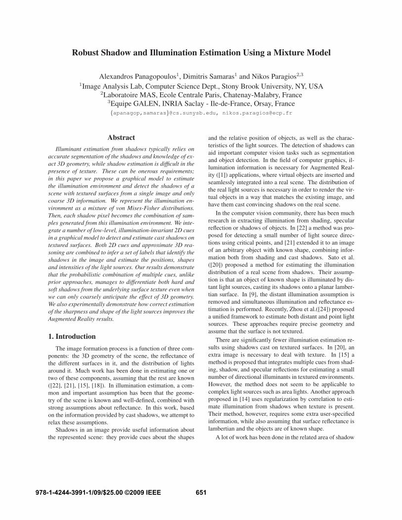
Figure 1. Illumination invariant images: a) original image, b) nor-

malized rgb, c) c1c2c3, d) the 1d illumination invariant image ob-

tained using the approach in [6]. Notice that in all three illumina-

tion invariant images, the shadow is much less visible than in the

original.

Having such a representation, we can compare gradients

in the original image with gradients in the illumination-

invariant representation to attribute the gradient to either

shadows/shading or texture. Having identified shadow bor-

ders this way, we can produce a set of labels identifying

shadows in the original image.

Illumination-invariant image cues are not sufficient in

the general case, however, and more complicated reason-

ing is necessary for more accurate shadow detection. An

example of this can be seen in figure 1, which shows the il-

lumination invariant features we use for an example image.

Edges due to illumination, although dimmer, are still noti-

cable, while some texture edges are not visible. Enforcing

consistency between the shadow and the scene geometry re-

moves many falsely detected shadow edges (fig.2).

4.1. Illumination­invariant cues

Photometric color invariants are functions which de-

scribe each image point, while disregarding shading and

shadows. These functions are demonstrated to be invari-

ant to a change in the imaging conditions, such as view-

ing direction, object’s surface orientation and illumination

conditions. Some examples of photometric invariant color

features are normalized RGB, hue, saturation, c1c2c3 and

l1l2l3 [7]. A more complicated illumination invariant rep-

resentation specifically targeted to shadows is described in

[6]. In this work, three illumination-invariant representa-

tions are integrated into our model: normalized rgb, c1c2c3

and the representation proposed in [6] (displayed in figure

1).

The c1c2c3 invariant color features are defined as:

ck(x, y) = arctanρk(x, y)

max(ρk+1mod3(x, y), ρk+2mod3(x, y))(10)

654

where ρk(x, y) is the k-th RGB color component for pixel

(x, y).

We only use the 1d illumination invariant representation

proposed in [6]. For this representation, a vector of illu-

minant variation e is estimated. The illumination invariant

features are defined as the projection of the log-chromaticity

vector x′ of the pixel color with respect to color channel p

to a vector e⊥ orthogonal to e:

I ′ = x′T e⊥ (11)

x′j =

ρk

ρp

, k ∈ 1, 2, 3, k 6= p, j = 1, 2 (12)

and ρk represents the k-th RGB component.

These illumination invariant features assume narrow-

band camera sensors, Planckian illuminants and a known

sensor response, which requires calibration. We circum-

vent the known sensor response requirement by using the

entropy-minimization procedure proposed in [5] to calcu-

late the illuminant variation direction e. Futhermore, it has

been shown that the features extracted this way are suffi-

ciently illumination-invariant, even if the other two assump-

tions above are not met ([6]).

Figure 1 shows the resulting illumination invariant im-

ages. It is easy to notice that some texture edges do not ap-

pear in the illumination invariant images in any of the repre-

sentations, especially in the case of edges between texture

patches with large intensity differences and similar color.

This leads to erroneously classifying some edges as shadow

borders. These false positives will be removed later in our

algorithm, utilizing the 3d reasoning about shadows.

4.2. Identifying shadow borders

A border which appears in the original image but not

in the illumination invariant images is a border which can

be attributed to illumination effects. Therefore, to identify

potential shadow borders, edges are detected in the origi-

nal image and each edge is checked against the illumination

invariant images. Calculating edges as simple finite differ-

ence approximations to gradients leads to a lot of noise, de-

tecting edges that are not important. To solve this, we apply

a smoothing filter to the original image, and then use the

Canny edge detector to detect edges.

We do not calculate similar edge maps from the illumi-

nation invariant images. Instead, for each pixel that lies on

an edge in the original image, we compare the difference

of the average values of the illumination invariants along

the direction of the gradient in the original image. Thus the

shadow border map is defined as:

es(x, y) =

{

1, if ‖∇I‖ > τ0 and |∆I(k)invar| < τk

0, otherwise

(13)

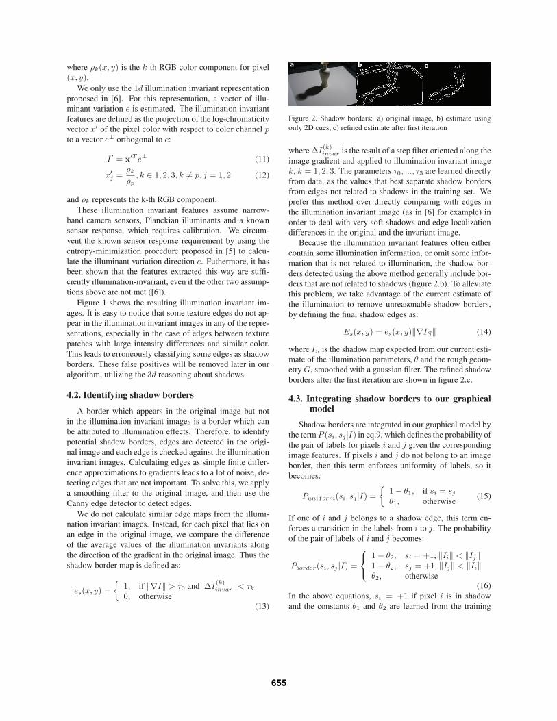
Figure 2. Shadow borders: a) original image, b) estimate using

only 2D cues, c) refined estimate after first iteration

where ∆I(k)invar is the result of a step filter oriented along the

image gradient and applied to illumination invariant image

k, k = 1, 2, 3. The parameters τ0, ..., τ3 are learned directly

from data, as the values that best separate shadow borders

from edges not related to shadows in the training set. We

prefer this method over directly comparing with edges in

the illumination invariant image (as in [6] for example) in

order to deal with very soft shadows and edge localization

differences in the original and the invariant image.

Because the illumination invariant features often either

contain some illumination information, or omit some infor-

mation that is not related to illumination, the shadow bor-

ders detected using the above method generally include bor-

ders that are not related to shadows (figure 2.b). To alleviate

this problem, we take advantage of the current estimate of

the illumination to remove unreasonable shadow borders,

by defining the final shadow edges as:

Es(x, y) = es(x, y)‖∇IS‖ (14)

where IS is the shadow map expected from our current esti-

mate of the illumination parameters, θ and the rough geom-

etry G, smoothed with a gaussian filter. The refined shadow

borders after the first iteration are shown in figure 2.c.

4.3. Integrating shadow borders to our graphicalmodel

Shadow borders are integrated in our graphical model by

the term P (si, sj |I) in eq.9, which defines the probability of

the pair of labels for pixels i and j given the corresponding

image features. If pixels i and j do not belong to an image

border, then this term enforces uniformity of labels, so it

becomes:

Puniform(si, sj |I) =

{

1− θ1, if si = sj

θ1, otherwise(15)

If one of i and j belongs to a shadow edge, this term en-

forces a transition in the labels from i to j. The probability

of the pair of labels of i and j becomes:

Pborder(si, sj |I) =

1− θ2, si = +1, ‖Ii‖ < ‖Ij‖1− θ2, sj = +1, ‖Ij‖ < ‖Ii‖θ2, otherwise

(16)

In the above equations, si = +1 if pixel i is in shadow

and the constants θ1 and θ2 are learned from the training

655

data. We do not assume that P (si, sj |I) has a distribution

dependent on the difference of the intensities of i and j in

order to make possible the detection of dim shadows. Often

the intensity changes over falsely detected shadow edges are

much larger than the ones over real shadow borders.

5. Estimating κ and intensity

Estimating the concentration parameter κ for a mixture

of vMF distributions requires significant approximations

([2]). In our model, it becomes even more difficult because

the values of the samples are not individually observed; in-

stead, only their per-pixel sums are known. It is easy to

observe, though, that there is a clear connection between

the shadow edge gradients, as they appear in the image,

and the concentration parameter of the light source distri-

butions. We exploit this connection to derive an estimator

for κ.

Let Ii

S be the image of the shadow intensities attributed

to light source distribution i. Assuming that the shadow

intensities are known, the relation connecting the gradient

of Ii

S and the parameter κi, using a linear approximation

for ex, is:

κi(x, y) ≥‖∇I

i

S(x, y)‖ −(∑

r∈R1o(r)−

∑

r∈R2o(r)

)

∑

r∈R1o(r)rµi −

∑

r∈R2o(r)rµi

(17)

where R1 and R2 are the samples at (x, y) and (x+∆x, y+∆y) respectively.

To estimate the true shadow image gradient∇Ii

S relevant

to light source distribution i, for each shadow edge pixel

(x, y), we project the image gradient along the direction of

the expected shadow gradient, ∇IiS , given the current illu-

mination estimate:

‖∇Ii

S(x, y)‖ =∇Ii

S(x, y)∇I(x, y)

αi‖∇IiS(x, y)‖

(18)

where αi is the current estimate of the intensity of light

source i. IiS has been smoothed using a gaussian filter.

To estimate κ, we compute the estimate from eq.17 for

all pixels located around the identified shadow borders. The

estimate of κi is selected to be the maximum of all per-pixel

estimates from eq.17. In practice, we discard the top 1% of

values as outliers and select the maximum of the remaining

values as the value of κi.

Intensity estimation is also based on shadow borders.

For each pixel (x, y) that lies on an identified shadow edge,

∇Ii

S(x, y) defines a direction perpendicular to the shadow

edge. We select two samples p1 = (x, y) + t1∇Ii

S(x, y)

and p2 = (x, y) + t2∇Ii

S(x, y). We increment t1 and t2

until we find a minimum of ∇Ii

S(p1) and ∇Ii

S(p2). Then

p1 lies in the shadow umbra and p2 is outside the shadow.

The intensity difference ∆I(x, y) = I(p2) − I(p1) is an

estimate of the shadow intensity. The light source intensity

0 5 10 15 20 250

5

10

15

20

25

30

iteration

an

gu

lar

err

or

(de

gre

es)

convergence

mean direction error, image 6.a

mean direction error, image 6.b

mean direction error, image 6.c

mean direction error, image 5.a

Figure 3. Convergence: the plot shows the mean error (in degrees)

between the estimated light source directions for each iteration and

the final parameter values from our algorithm

Figure 4. Comparison of real and synthesized shadows: a,b) pho-

tographs under same illumination, c) estimated illumination from

(a), d) a picture of the background with the object removed, e) a

3D model of the original object rendered with the estimated illu-

mination, and superimposed on the background image of (c). The

shadows in this image are rendered with the estimated illumination

and cast on the background image.

αi is set to the mean of all ∆I(x, y), for shadow edge pixels

(x, y). Intensities are normalized so that∑

i αi = 1.

6. Results

For all of our experiments, 200 random samples of the

illumination sphere per pixel were used. A maximum of

40 EM iterations and 1500 iterations for the belief propaga-

tion in the factor graph were performed. The average run-

ning time of the algorithm was 3-5 minutes per image (For

performance reasons, several EM iterations were performed

before successive applications of belief propagation in the

E-step). On average, our algorithm needed 15 to 20 EM it-

erations per light source distribution to converge (see Fig.3).

656

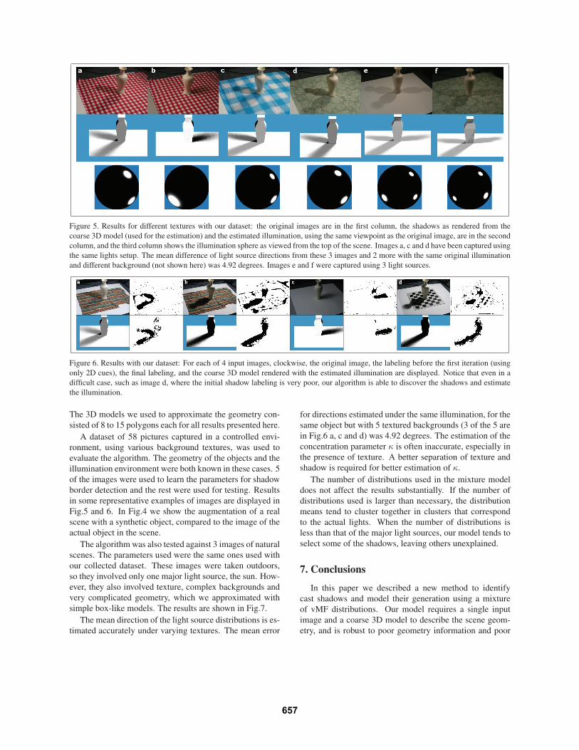
Figure 5. Results for different textures with our dataset: the original images are in the first column, the shadows as rendered from the

coarse 3D model (used for the estimation) and the estimated illumination, using the same viewpoint as the original image, are in the second

column, and the third column shows the illumination sphere as viewed from the top of the scene. Images a, c and d have been captured using

the same lights setup. The mean difference of light source directions from these 3 images and 2 more with the same original illumination

and different background (not shown here) was 4.92 degrees. Images e and f were captured using 3 light sources.

Figure 6. Results with our dataset: For each of 4 input images, clockwise, the original image, the labeling before the first iteration (using

only 2D cues), the final labeling, and the coarse 3D model rendered with the estimated illumination are displayed. Notice that even in a

difficult case, such as image d, where the initial shadow labeling is very poor, our algorithm is able to discover the shadows and estimate

the illumination.

The 3D models we used to approximate the geometry con-

sisted of 8 to 15 polygons each for all results presented here.

A dataset of 58 pictures captured in a controlled envi-

ronment, using various background textures, was used to

evaluate the algorithm. The geometry of the objects and the

illumination environment were both known in these cases. 5

of the images were used to learn the parameters for shadow

border detection and the rest were used for testing. Results

in some representative examples of images are displayed in

Fig.5 and 6. In Fig.4 we show the augmentation of a real

scene with a synthetic object, compared to the image of the

actual object in the scene.

The algorithm was also tested against 3 images of natural

scenes. The parameters used were the same ones used with

our collected dataset. These images were taken outdoors,

so they involved only one major light source, the sun. How-

ever, they also involved texture, complex backgrounds and

very complicated geometry, which we approximated with

simple box-like models. The results are shown in Fig.7.

The mean direction of the light source distributions is es-

timated accurately under varying textures. The mean error

for directions estimated under the same illumination, for the

same object but with 5 textured backgrounds (3 of the 5 are

in Fig.6 a, c and d) was 4.92 degrees. The estimation of the

concentration parameter κ is often inaccurate, especially in

the presence of texture. A better separation of texture and

shadow is required for better estimation of κ.

The number of distributions used in the mixture model

does not affect the results substantially. If the number of

distributions used is larger than necessary, the distribution

means tend to cluster together in clusters that correspond

to the actual lights. When the number of distributions is

less than that of the major light sources, our model tends to

select some of the shadows, leaving others unexplained.

7. Conclusions

In this paper we described a new method to identify

cast shadows and model their generation using a mixture

of vMF distributions. Our model requires a single input

image and a coarse 3D model to describe the scene geom-

etry, and is robust to poor geometry information and poor

657

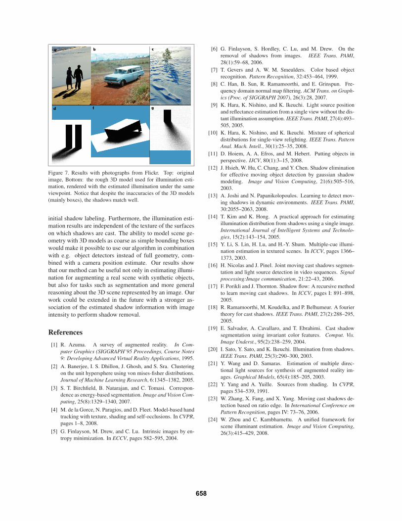
Figure 7. Results with photographs from Flickr. Top: original

image, Bottom: the rough 3D model used for illumination esti-

mation, rendered with the estimated illumination under the same

viewpoint. Notice that despite the inaccuracies of the 3D models

(mainly boxes), the shadows match well.

initial shadow labeling. Furthermore, the illumination esti-

mation results are independent of the texture of the surfaces

on which shadows are cast. The ability to model scene ge-

ometry with 3D models as coarse as simple bounding boxes

would make it possible to use our algorithm in combination

with e.g. object detectors instead of full geometry, com-

bined with a camera position estimate. Our results show

that our method can be useful not only in estimating illumi-

nation for augmenting a real scene with synthetic objects,

but also for tasks such as segmentation and more general

reasoning about the 3D scene represented by an image. Our

work could be extended in the future with a stronger as-

sociation of the estimated shadow information with image

intensity to perform shadow removal.

References

[1] R. Azuma. A survey of augmented reality. In Com-

puter Graphics (SIGGRAPH’95 Proceedings, Course Notes

9: Developing Advanced Virtual Reality Applications, 1995.

[2] A. Banerjee, I. S. Dhillon, J. Ghosh, and S. Sra. Clustering

on the unit hypersphere using von mises-fisher distributions.

Journal of Machine Learning Research, 6:1345–1382, 2005.

[3] S. T. Birchfield, B. Natarajan, and C. Tomasi. Correspon-

dence as energy-based segmentation. Image and Vision Com-

puting, 25(8):1329–1340, 2007.

[4] M. de la Gorce, N. Paragios, and D. Fleet. Model-based hand

tracking with texture, shading and self-occlusions. In CVPR,

pages 1–8, 2008.

[5] G. Finlayson, M. Drew, and C. Lu. Intrinsic images by en-

tropy minimization. In ECCV, pages 582–595, 2004.

[6] G. Finlayson, S. Hordley, C. Lu, and M. Drew. On the

removal of shadows from images. IEEE Trans. PAMI,

28(1):59–68, 2006.

[7] T. Gevers and A. W. M. Smeulders. Color based object

recognition. Pattern Recognition, 32:453–464, 1999.

[8] C. Han, B. Sun, R. Ramamoorthi, and E. Grinspun. Fre-

quency domain normal map filtering. ACM Trans. on Graph-

ics (Proc. of SIGGRAPH 2007), 26(3):28, 2007.

[9] K. Hara, K. Nishino, and K. Ikeuchi. Light source position

and reflectance estimation from a single view without the dis-

tant illumination assumption. IEEE Trans. PAMI, 27(4):493–

505, 2005.

[10] K. Hara, K. Nishino, and K. Ikeuchi. Mixture of spherical

distributions for single-view relighting. IEEE Trans. Pattern

Anal. Mach. Intell., 30(1):25–35, 2008.

[11] D. Hoiem, A. A. Efros, and M. Hebert. Putting objects in

perspective. IJCV, 80(1):3–15, 2008.

[12] J. Hsieh, W. Hu, C. Chang, and Y. Chen. Shadow elimination

for effective moving object detection by gaussian shadow

modeling. Image and Vision Computing, 21(6):505–516,

2003.

[13] A. Joshi and N. Papanikolopoulos. Learning to detect mov-

ing shadows in dynamic environments. IEEE Trans. PAMI,

30:2055–2063, 2008.

[14] T. Kim and K. Hong. A practical approach for estimating

illumination distribution from shadows using a single image.

International Journal of Intelligent Systems and Technolo-

gies, 15(2):143–154, 2005.

[15] Y. Li, S. Lin, H. Lu, and H.-Y. Shum. Multiple-cue illumi-

nation estimation in textured scenes. In ICCV, pages 1366–

1373, 2003.

[16] H. Nicolas and J. Pinel. Joint moving cast shadows segmen-

tation and light source detection in video sequences. Signal

processing:Image communication, 21:22–43, 2006.

[17] F. Porikli and J. Thornton. Shadow flow: A recursive method

to learn moving cast shadows. In ICCV, pages I: 891–898,

2005.

[18] R. Ramamoorthi, M. Koudelka, and P. Belhumeur. A fourier

theory for cast shadows. IEEE Trans. PAMI, 27(2):288–295,

2005.

[19] E. Salvador, A. Cavallaro, and T. Ebrahimi. Cast shadow

segmentation using invariant color features. Comput. Vis.

Image Underst., 95(2):238–259, 2004.

[20] I. Sato, Y. Sato, and K. Ikeuchi. Illumination from shadows.

IEEE Trans. PAMI, 25(3):290–300, 2003.

[21] Y. Wang and D. Samaras. Estimation of multiple direc-

tional light sources for synthesis of augmented reality im-

ages. Graphical Models, 65(4):185–205, 2003.

[22] Y. Yang and A. Yuille. Sources from shading. In CVPR,

pages 534–539, 1991.

[23] W. Zhang, X. Fang, and X. Yang. Moving cast shadows de-

tection based on ratio edge. In International Conference on

Pattern Recognition, pages IV: 73–76, 2006.

[24] W. Zhou and C. Kambhamettu. A unified framework for

scene illuminant estimation. Image and Vision Computing,

26(3):415–429, 2008.

658