Embed Size (px)
Citation preview
Robust Semidefinite Programming∗
Aharon Ben-Tal† Laurent El Ghaoui‡ Arkadi Nemirovski§
August 1st, 1998
AbstractIn this paper, we consider semidefinite programs where the data is only known to belong
to some uncertainty set U . Following recent work by the authors, we develop the notion ofrobust solution to such problems, which are required to satisfy the (uncertain) constraintswhatever the value of the data in U . Even when the decision variable is fixed, checkingrobust feasibility is in general NP-hard. For a number of uncertainty sets U , we showhow to compute robust solutions, based on a sufficient condition for robust feasibility, viaSDP. We detail some cases when the sufficient condition is also necessary, such as linearprogramming or convex quadratic programming with ellipsoidal uncertainty. Finally, weprovide examples, taken from interval computations and truss topology design.
1 Introduction
1.1 SDPs with uncertain data
We consider a semidefinite programming problem (SDP) of the form
max bT y subject to F (y) = F0 +m∑
i=1
yiFi º 0, (1)
where b ∈ Rm is given, and F is an affine map from y ∈ Rm to Sn.In many practical applications, the “data” of the problem (the vector b and the coefficients matrices
F0, . . . , Fm) is subject to possibly large uncertainties. Reasons for this include the following.
• Uncertainty about the future. The exact value of the data is unknown at the time the values of yshould be determined and will be known only in the future. (In a risk management problem forexample, the data may depend on future demands, market prices, etc, that are unknown whenthe decision has to be taken.)
∗This research was partly supported by the Fund for the Promotion of Research at the Technion, by the G.I.F.contract No. I-0455-214.06/95, by the Israel Ministry of Science grant # 9636-1-96, and by Electricite de France, undercontract P33L74/2M7570/EP777.
†Faculty of Industrial Engineering and Management, Technion – The Israel Institute of Technology, Technion City,Haifa 32000, Israel; e-mail: [email protected]
‡Ecole Nationale Suprieure de Techniques Avances, 32, Bvd. Victor, 75739 Paris, France; email: [email protected].§Faculty of Industrial Engineering and Management, Technion - The Israel Institute of Technology, Technion City,
Haifa 32000, Israel; e-mail: [email protected]
1
• Errors in the data. The data originates from a process (measurements, computational process)that is very hard to perform error-free (errors in the measurement of material properties in atruss optimization problem, sensor errors in a control system, floating-point errors made duringcomputation, etc).
• Implementation errors. The computed optimal solution y∗ cannot be implemented exactly,which results in uncertainty about the feasibility of the implemented solution. For example, thecoefficients of an optimal finite-impulse response (FIR) filter can often be implemented in 8 bitsonly. As it turns out, this can be modeled as uncertainties in the coefficients matrices Fi.
• Approximating nonlinearity by uncertainty. The mapping F (y) is completely known, but (slightly)non linear. The optimizer chooses to approximate the nonlinearity by uncertainty in the data.
• Infinite number of constraints. The problem is posed with an infinite number of constraints,indexed on a scalar parameter ω (for example, the constraints express a property of a FIR filterat each frequency ω). It may be convenient to view this parameter as a perturbation, and regardthe semi-infinite problem as a robustness problem.
Depending on the assumptions on the nature of uncertainty, several methods have been proposedin the Operations Research/Engineering literature. Stochastic programming works with random per-turbations and probabilities of satisfaction of constraints, and thus requires correct estimates of thedistribution of uncertainties; sensitivity analysis assumes the perturbations is infinitesimal, and canbe used only as a “post-optimization” tool; the “Robust Mathematical Programming” approach re-cently proposed by Mulvey, Vanderbei and Zenios [13] is based on the (sometimes very restrictive)assumption that the uncertainty takes a finite number of values (corresponding to “worst-case scenar-ios”). Interval arithmetic is one of the methods that have been proposed to deal with uncertainty innumerical computations; references to this large field of study include the book by one of its founders,Moore [12], the more recent book by Hansen [9], and also the very extensive web site developed byKosheler and Kreinovich [11].
The approach proposed here assumes (following the philosophy of interval calculus) that the dataof the problem is only known to belong to some “uncertainty set” U ; in this sense, the perturbationto the nominal problem is deterministic, unknown-but-bounded. A robust solution of the problem isone which satisfies the perturbed constraints for every value of the data within the admissible regionU . The robust counterpart of the SDP is to minimize the worst-case value of the objective, among allrobust solutions. This approach was introduced by the authors independently in [1, 2, 3] and [15, 5];although apparently new in mathematical programming, the notion of robustness is quite classical incontrol theory (and practice).
Even for simple uncertainty sets U , the resulting robust SDP is NP-hard. Our main result is to showhow to compute, via SDP, upper bounds for the robust counterpart. Contrarily to the other approachesto uncertainty, the robust method provides (in polynomial time) guarantees (of,e.g., feasibility), atthe expense of possible conservatism. Note that there is no real conflict between other approaches touncertainty and ours; for example, it is possible to solve via robust SDP a stochastic programmingproblem with unknown-but-bounded distribution of the random parameters.
1.2 Problem definition
To make our problem mathematically precise, we assume that the perturbed constraint is of the form
F(y, δ) º 0,
2
where y ∈ Rm is the decision vector, δ is a “perturbation vector” that is only known to belong tosome “perturbation set” D ⊆ Rl, and F is a mapping from Rm × D to Sn. We assume that F(y, δ)is affine in y for each δ, and rational in δ for each y; also we assume that D contains 0, and thatF(y, 0) = F (y) for every y. Without loss of generality, we assume that the objective vector b isindependent of perturbation.
We consider the following problem, referred to as the robust counterpart to the “nominal” prob-lem (1):
max bT y subject to y ∈ XD (2)
where XD is the set of robust feasible solutions, that is,
XD ={y ∈ Rm
∣∣∣ for every δ ∈ D, F(y, δ) is well-defined and F(y, δ) º 0}
.
In this paper, we only consider ellipsoidal uncertainty. This means that the perturbation set Dconsists of block vectors, each block being subject to an Euclidean-norm bound. Precisely,
D =
δ ∈ Rl
∣∣∣∣∣∣∣δ =
δ1
...δN
, where δk ∈ Rnk , ‖δk‖2 ≤ ρ, k = 1, . . . , N
, (3)
where ρ ≥ 0 is a given parameter that determines the “size” of the uncertainty, and the integers nk
denote the lengths of each block vector δk (we have of course n1 + . . . + nN = L).There are many motivations for considering the above framework. It can be used when the per-
turbation is a vector with each component bounded in magnitude, in which case each block vector δk
is actually a scalar (n1 = . . . = nN = 1). It also can be used when the perturbation is bounded in Eu-clidean norm (which is often the case when the bounds on the parameters are obtained from statistics,and a Gaussian distribution is assumed). In some applications, there is a mixture of Euclidean-normand maximum-norm bounds. (For example, we might have some parameters of the form δ1 = ρ cos θ,δ2 = ρ sin θ, where both ρ and θ are uncertain.)
It turns out that already in the case of affine perturbations (F(·, δ) is affine in δ) the robustcounterpart (2), generally speaking, is NP-hard. This is why we are interested not only in the robustcounterpart itself, but also in its approximations – “computationally tractable” problems with thesame objective as in (2) and feasible sets contained in the set XD of robust solutions. We will obtainan upper bound (approximation) on the robust counterpart in the form of an SDP. The size of thisSDP is linear in both the length nk of each block and the number N of blocks.
The paper is organized as follows. In section 2, we consider the case when the perturbation vectoraffects the semidefinite constraint affinely, that is, the matrix F(y, δ) is affine in δ; we provide not onlyan approximation of the robust counterpart, but also a result on the quality of the approximation,in an appropriately defined sense. Section 3 is devoted to the general case (the perturbation δ entersrationally in F(y, δ)). We provide interesting special cases (when the approximation is exact) insection 4, while section 5 describes several examples of application.
2 Affine perturbations
In this section, we assume that the matrix function F(y, δ) is given by
F(y, δ) = F 0(y) +l∑
i=1
δiFi(y) (4)
3

where each F i(y) is a symmetric matrix, affine in y.We have the following result.
Theorem 2.1 Consider uncertain semidefinite program with affine perturbation (4) and ellipsoidaluncertainty (3), and let ν0 = 0, νk =
∑ks=1 ns. Then the semidefinite program
max bT ys.t.
(a)
Sk ρFνk−1+1(y) ρFνk−1+2(y) · · · ρFνk(y)
ρFνk−1+1(y) Qk
ρFνk−1+2(y) Qk...
. . ....
ρFνk(y) Qk
º 0, k = 1, 2, . . . , N ;
(b)∑N
k=1(Sk + Qk) ¹ 2F0(y);
(5)
in variables y, S1, . . . , SN , Q1, . . . , QN is an approximation of the robust counterpart (2), i.e., theprojection of the feasible set of (5) on the space of y-variables is contained in the set of robust feasiblesolutions.
Proof. Let us fix a feasible solution Y = (y, {Sk}, {Qk}) to (5), and let us set Fi = Fi(y). We should provethat
(*) For every δ = {δi}li=1 such that
νk∑
i=νk−1+1
δ2i ≤ ρ2, k = 1, . . . , N, (6)
one hasF0 +
∑
i
δiFi º 0.
Since Y is feasible for (5), it follows that the matrices F0, S1, . . . , SN , Q1, . . . , QN are positive semidefinite.By obvious regularization arguments, we may further assume these matrices to be positive definite. Finally,performing “scaling”
Sk 7→ F−1/20 SkF
−1/20 ,
Qk 7→ F−1/20 QkF
−1/20 ,
Fi 7→ F−1/20 FiF
−1/20 ,
Φ0 7→ I,
we reduce the situation to the one where F0 = I, which we assume till the end of the proof.Let Ik be the set of indices νk−1 + 1, . . . , νk. Whenever δ satisfies (6) and ξ ∈ Rn, n being the row size of
4
Fi’s, we have
ξT (I +∑
i δiFi) ξ = ξT ξ +∑
k
[Q
1/2k ξ
]T [∑i∈Ik
δiQ−1/2k FiS
−1/2k ξk
]
[ξk = S1/2k ξ, k = 1, . . . , N ]
≥ ξT ξ −∑k ‖Q1/2
k ξ‖2[∑
i∈Ik|δi|‖Q−1/2
k FiS−1/2k ξk‖2
]
≥ ξT ξ −∑k ‖Q1/2
k ξ‖2√∑
i∈Ikρ2‖Q−1/2
k FiS−1/2k ξk‖22
[we have used (6)]
= ξT ξ −∑k ‖Q1/2
k ξ‖2√
ρ2ξTk
[∑i∈Ik
S−1/2k FiQ
−1k FiS
−1/2k
]ξk
≥ ξT ξ −∑k ‖Q1/2
k ξ‖2√
ξTk ξk
[we have used (5.a)]
≥ ξT ξ −√∑
k ‖Q1/2k ξ‖22
√∑k ξT
k ξk
= ξT ξ −√ξT [
∑k Qk] ξ
√ξT [
∑k Sk] ξ
(7)
It remains to note that if a = ξT [∑
k Qk] ξ, b = ξT [∑
k Sk] ξ, then a + b ≤ 2ξT ξ by (5.b) (recall that we are inthe situation F0(y) = I), so that
√ab ≤ ξT ξ. Thus, the concluding expression in (7) is nonnegative.
2.1 Quality of approximation
A general-type approximation of the robust counterpart (2) is an optimization problem
max bT y subject to (y, z) ∈ Y (A)
(with variables y, z) such that the projection X (A) of its feasible set Y on the space of y-variablesis contained in XD, so that (A)-feasibility of (y, z) implies robust feasibility of y. For a particularapproximation, a question of primary interest is how conservative the approximation is. A naturalway to measure the “level of conservativeness” of an approximation (A) is as follows. Since (A) is anapproximation of (2), we have X (A) ⊂ XD. Now let us increase the level of perturbations, i.e., let usreplace the original set of perturbations D by its κ-enlargement κD, κ ≥ 1. The set XκD of robustfeasible solutions associated with the enlarged set of perturbations shrinks as κ grows, and for largeenough values of κ it may become a part of X (A). The lower bound of these “large enough” values ofκ can be treated as the level of conservativeness λ(A) of the approximation (A):
λ(A) = inf{κ ≥ 1 : XκD ⊂ X (A)}.Thus, we say that the level of conservativeness of an approximation (A) is < λ, if every y which is“rejected” by (A) (i.e., y 6∈ X (A)) looses robust feasibility after the level ρ of perturbations in (3) isincreased by factor λ.
The following theorem bounds the level of conservativeness of approximations we have derived sofar:
Theorem 2.2 Consider semidefinite program with affine perturbations (4) and ellipsoidal uncertainty(3), the blocks δk of the perturbation vector being of dimensions nk, k = 1, . . . , N , and let l =
∑k nk
and n be the row size of F (·, ·). The level of conservativeness of the approximation (5) does not exceedmin
[√nN ;
√l].
Proof. Of course, it suffices to consider the case of ρ = 1, which is assumed till the end of the proof.Let X be the projection of the feasible set of (5) to the space of y-variables, and let y 6∈ X . We should prove
that y 6∈ XλD at least in the following two cases:
5
(i.1): λ >√
l; (i.2): λ >√
nN .To save notation, let us write Fi instead of Fi(y). Note that we may assume that F0 º 0 – otherwise y is notrobust feasible and there is nothing to prove. In fact we may assume even F0 Â 0, since from the structure of(5) it is clear that the relation y 6∈ X , being valid for the original data F0, . . . , Fl, remains valid when we replacea positive semidefinite matrix F0 with a close positive definite matrix. Note that this regularization may onlyincrease the robust feasible set, so that it suffices to prove the statement in question in the case of F0 Â 0.Finally, the same scaling as in the proof of Theorem 2.1 allows to assume that F0 = I. Let also Ik be the sameindex sets as in the proof of Theorem 2.1.
10. Consider the case of (i.1). Let us set
Qk = nk
l I,
Sk = lnk
∑i∈Ik
F 2i .
The collection (y, {Sk, Qk}) clearly satisfies (5.a, c), and therefore it must violate (5.b), since otherwise we wouldhave y ∈ X . Thus, there exists an n-dimensional vector ξ such that
N∑
k=1
l
nk
∑
i∈Ik
‖Fiξ‖22 > ξT ξ. (8)
Settingpk = max
i∈Ik
‖Fiξ‖2 = ‖Fikξ‖2, ik ∈ Ik,
we come toN∑
k=1
lp2k > ξT ξ. (9)
Now let δ ∈ λD be a random vector with independent coordinates distributed as follows: a coordinate δi withindex i ∈ Ik is zero, except the case of i = ik, and the coordinate δik
takes values ±λ with probabilities 1/2.The expected squared Euclidean norm of the random vector
∑i δiFiξ clearly is equal to λ2
∑k p2
k; thus, λDcontains a perturbation δ such that
‖[
l∑
i=1
δiFi
]ξ‖22 ≥ λ2
∑
k
p2k > λ2l−1ξT ξ;
since λ2l−1 > 1 by (i.1), we conclude that the spectral norm of the matrix∑
i δiFi is > 1, whence either thismatrix, or its negation is not ¹ F0 = I. Thus, y 6∈ XλD, as claimed.
20. Now let (i.2) be the case. Let us set
Qk = N−1I,Sk = N
∑i∈Ik
F 2i .
By the same reasons as in 10, there exists an n-dimensional vector ξ such that
N∑
k=1
N∑
i∈Ik
‖Fiξ‖22 > ξT ξ. (10)
Denoting e1, . . . , en the standard basic orths in Rn, we conclude that there exists p ∈ {1, . . . n} such that
N∑
k=1
N∑
i∈Ik
|eTp Fiξ|2 >
1n
ξT ξ. (11)
We clearly can choose δ ∈ λD in such a way that
∑
i∈Ik
δieTp Fiξ = λ
√∑
i∈Ik
|eTp Fiξ|2.
6
SettingF =
∑
i
δiFi,
we geteTp Fξ =
∑k
∑i∈Ik
eTp δiFiξ
≥ λ∑N
k=1
√∑i∈Ik
|eTp Fiξ|2
≥ λ√∑N
k=1
∑i∈Ik
|eTp Fiξ|2
> λ√mN
‖ξ‖2 [see (11)]> ‖ξ‖2 [by (i.2)]
We conclude that the spectral norm of F is > 1, so that either F or −F is not º F0 = I. Thus, y 6∈ XλD, asclaimed.
3 Rational Dependence
In this section, we seek to handle cases when the matrix-valued function F(y, δ) is rational in δ forevery y. There are many practical situations when the perturbation parameters enter rationally, andnot affinely, in a perturbed SDP. One important example arises with the problem of checking robustsingularity of a square (non symmetric) matrix A, which depends affinely on parameters. One has tocheck if ATA Â 0 for every A in the affine uncertainty set; this is a matrix inequality condition inwhich the parameters enter quadratically.
We will introduce a versatile framework, called linear-fractional representations, for describing ra-tional dependence, and devise approximate robust counterparts that are based on this linear-fractionalrepresentation. Our framework will of course cover the cases when the perturbation enters affinelyin the matrix F(y, δ), which is a case already covered by theorem 2.1. At present we do not know iftheorem 2.1 always yields more accurate results than those described next, except in the case N = 1(Euclidean-norm bounds), where both results are actually equivalent.
In this section, we take ρ = 1.
3.1 Linear-fractional representations
We assume that the function F is given by a “linear-fractional representation” (LFR):
F(y, ∆) = F (y) + L(y)∆(I −D∆)−1R + RT (I −∆T DT )−1∆T L(y)T , (a)∆ = diag (δ1Ir1 , . . . , δlIrl
) ,
where F (y) is defined in (1), L(·) is an affine mapping taking values in Rn×p, R ∈ Rq×n and D ∈ Rq×p
are given matrices, and r1, . . . , rl are given integers. We assume that the above LFR is well-posedover D, meaning that det(I −D∆) for every ∆ of the form above, with δ ∈ D; we return to the issueof well-posedness later.
The above class of models seem quite specialized. In fact, these models can be used in a widevariety of situations. For example, in the case of affine dependence:
F(δ) = F 0(y) +l∑
i=1
δiFi(y),
7
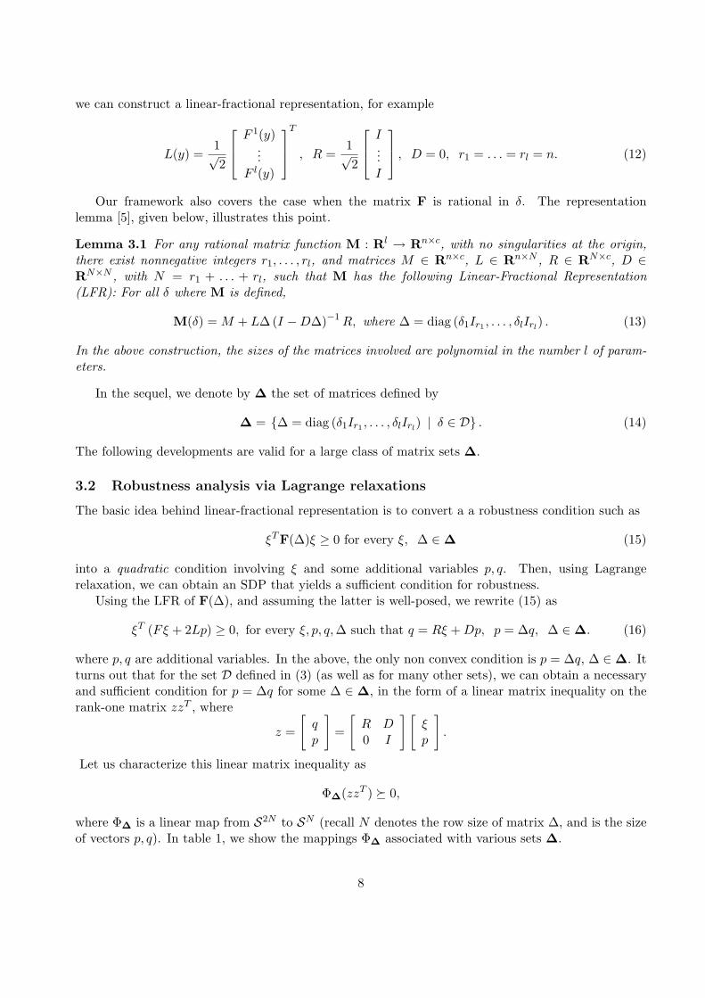
we can construct a linear-fractional representation, for example
L(y) =1√2
F 1(y)...
F l(y)
T
, R =1√2
I...I
, D = 0, r1 = . . . = rl = n. (12)
Our framework also covers the case when the matrix F is rational in δ. The representationlemma [5], given below, illustrates this point.
Lemma 3.1 For any rational matrix function M : Rl → Rn×c, with no singularities at the origin,there exist nonnegative integers r1, . . . , rl, and matrices M ∈ Rn×c, L ∈ Rn×N , R ∈ RN×c, D ∈RN×N , with N = r1 + . . . + rl, such that M has the following Linear-Fractional Representation(LFR): For all δ where M is defined,
M(δ) = M + L∆(I −D∆)−1 R, where ∆ = diag (δ1Ir1 , . . . , δlIrl) . (13)
In the above construction, the sizes of the matrices involved are polynomial in the number l of param-eters.
In the sequel, we denote by ∆ the set of matrices defined by
∆ = {∆ = diag (δ1Ir1 , . . . , δlIrl) | δ ∈ D} . (14)
The following developments are valid for a large class of matrix sets ∆.
3.2 Robustness analysis via Lagrange relaxations
The basic idea behind linear-fractional representation is to convert a a robustness condition such as
ξTF(∆)ξ ≥ 0 for every ξ, ∆ ∈ ∆ (15)
into a quadratic condition involving ξ and some additional variables p, q. Then, using Lagrangerelaxation, we can obtain an SDP that yields a sufficient condition for robustness.
Using the LFR of F(∆), and assuming the latter is well-posed, we rewrite (15) as
ξT (Fξ + 2Lp) ≥ 0, for every ξ, p, q, ∆ such that q = Rξ + Dp, p = ∆q, ∆ ∈ ∆. (16)
where p, q are additional variables. In the above, the only non convex condition is p = ∆q, ∆ ∈ ∆. Itturns out that for the set D defined in (3) (as well as for many other sets), we can obtain a necessaryand sufficient condition for p = ∆q for some ∆ ∈ ∆, in the form of a linear matrix inequality on therank-one matrix zzT , where
z =
[qp
]=
[R D0 I
] [ξp
].
Let us characterize this linear matrix inequality as
Φ∆(zzT ) º 0,
where Φ∆ is a linear map from S2N to SN (recall N denotes the row size of matrix ∆, and is the sizeof vectors p, q). In table 1, we show the mappings Φ∆ associated with various sets ∆.
8
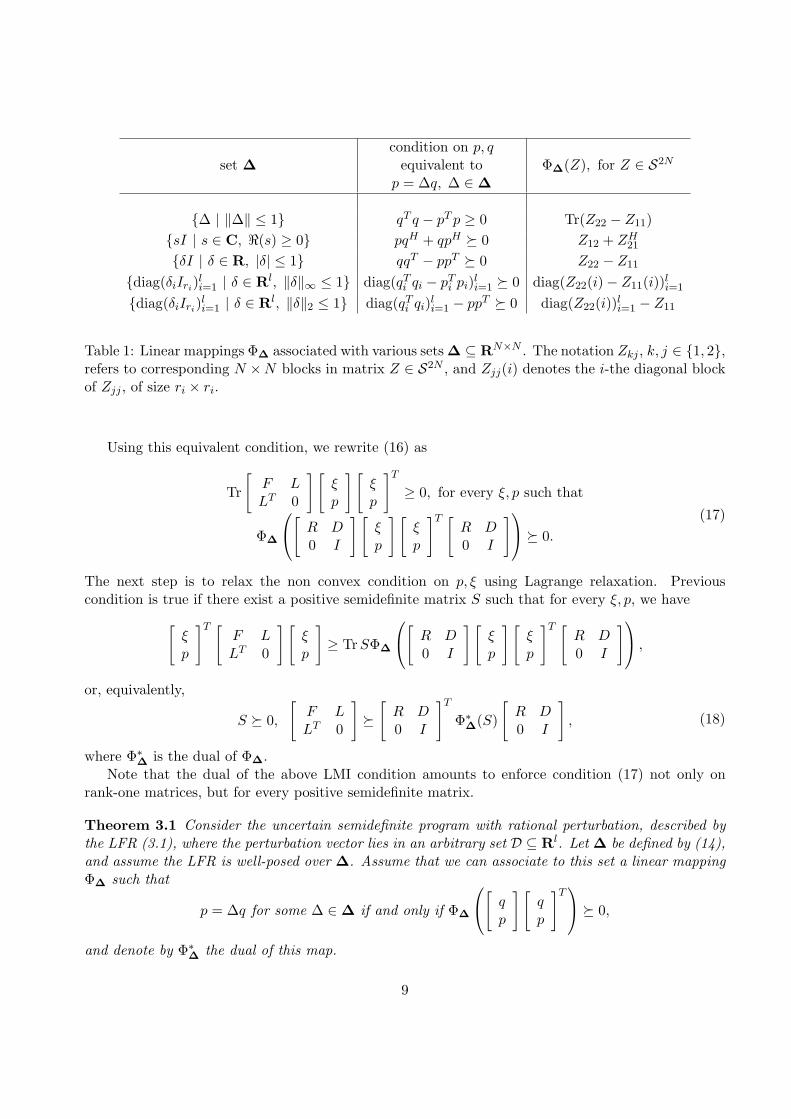
set ∆condition on p, q
equivalent top = ∆q, ∆ ∈ ∆
Φ∆(Z), for Z ∈ S2N
{∆ | ‖∆‖ ≤ 1} qT q − pT p ≥ 0 Tr(Z22 − Z11){sI | s ∈ C, <(s) ≥ 0} pqH + qpH º 0 Z12 + ZH
21
{δI | δ ∈ R, |δ| ≤ 1} qqT − ppT º 0 Z22 − Z11
{diag(δiIri)li=1 | δ ∈ Rl, ‖δ‖∞ ≤ 1} diag(qT
i qi − pTi pi)l
i=1 º 0 diag(Z22(i)− Z11(i))li=1
{diag(δiIri)li=1 | δ ∈ Rl, ‖δ‖2 ≤ 1} diag(qT
i qi)li=1 − ppT º 0 diag(Z22(i))l
i=1 − Z11
Table 1: Linear mappings Φ∆ associated with various sets ∆ ⊆ RN×N . The notation Zkj , k, j ∈ {1, 2},refers to corresponding N ×N blocks in matrix Z ∈ S2N , and Zjj(i) denotes the i-the diagonal blockof Zjj , of size ri × ri.
Using this equivalent condition, we rewrite (16) as
Tr
[F LLT 0
] [ξp
] [ξp
]T
≥ 0, for every ξ, p such that
Φ∆
[R D0 I
] [ξp
] [ξp
]T [R D0 I
] º 0.
(17)
The next step is to relax the non convex condition on p, ξ using Lagrange relaxation. Previouscondition is true if there exist a positive semidefinite matrix S such that for every ξ, p, we have
[ξp
]T [F LLT 0
] [ξp
]≥ TrSΦ∆
[R D0 I
] [ξp
] [ξp
]T [R D0 I
] ,
or, equivalently,
S º 0,
[F LLT 0
]º
[R D0 I
]T
Φ∗∆(S)
[R D0 I
], (18)
where Φ∗∆ is the dual of Φ∆.Note that the dual of the above LMI condition amounts to enforce condition (17) not only on
rank-one matrices, but for every positive semidefinite matrix.
Theorem 3.1 Consider the uncertain semidefinite program with rational perturbation, described bythe LFR (3.1), where the perturbation vector lies in an arbitrary set D ⊆ Rl. Let ∆ be defined by (14),and assume the LFR is well-posed over ∆. Assume that we can associate to this set a linear mappingΦ∆ such that
p = ∆q for some ∆ ∈ ∆ if and only if Φ∆
[qp
] [qp
]T º 0,
and denote by Φ∗∆ the dual of this map.
9
Then the semidefinite program
max bT y subject to
S º 0,
[F (y) L(y)L(y)T 0
]º
[R D0 I
]T
Φ∗∆(S)
[R D0 I
]
in variables y, S, is an approximation of the robust counterpart (2), i.e., the projection of the feasibleset of (2) on the space of y-variables is contained in the set of robust feasible solutions.
It is now a simple matter to specialize the above result for the set D defined in (3). The conditionon p, q that is equivalent to p = ∆q, ∆ ∈ ∆ writes
diag(qiqTi )i∈Ik
− pk(pk)T º 0 k = 1, . . . , N, (19)
where Ik be the set of indices νk−1 + 1, . . . , νk, with ν0 = 0, νk =∑k
s=1 ns, and pk is the vector withelements (pi)i∈Ik
.The following result is then a corollary of theorem 3.1.
Corollary 3.1 Consider the uncertain semidefinite program with rational perturbation, described bythe LFR (3.1), where the perturbation vector lies in the set D defined in (3). Let ∆ be defined by (14),and assume the LFR is well-posed over ∆.
Consider the semidefinite program
max bT y subject to S º 0,[F (y) L(y)L(y)T 0
]º
[R D0 I
]T [T 00 −S
] [R D0 I
](20)
where S = diag(S1, . . . , SN ), with each Si of size∑
i∈Ikri, and T is the block-diagonal matrix formed
with the block-diagonal ri × ri blocks of S.Then the above semidefinite program in variables y, S, is an approximation of the robust counterpart
(2), i.e., the projection of the feasible set of (2) on the space of y-variables is contained in the set ofrobust feasible solutions.
Remark 3.1 We note that the above condition, if it is strictly enforced, ensures well-posedness, mean-ing that det(I−D∆) 6= 0 for every ∆ ∈ ∆. (To prove this, it suffices to apply the previous methodologyto the matrix function F(∆) = (I −D∆)T (I −D∆).)
3.3 Comparison with earlier results
We do not have a general comparison theorem with the results of section 2, in the case of affinedependence. However, we can prove that, when D represents Euclidean-norm bounds (that is, thereis only one block: N = 1), then both results are equivalent.
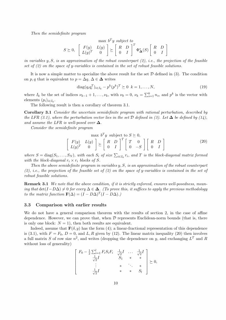
Indeed, assume that F(δ, y) has the form (4); a linear-fractional representation of this dependenceis (3.1), with F = F0, D = 0, and L,R given by (12). The linear matrix inequality (20) then involvesa full matrix S of row size n2, and writes (dropping the dependence on y, and exchanging LT and Rwithout loss of generality)
F0 − 12
∑li=1 FiSiFi
1√2I . . . 1√
2I
1√2I S1 ∗ ∗
... ∗ . . . ∗1√2I ∗ ∗ Sl
º 0,
10

where Si are the n× n diagonal blocks of S, and the symbols ∗ refer to the other blocks of S. Usingthe elimination lemma [4], it is possible to get rid of these elements and rewrite the above as
[F0 − 1
2
∑i=1 FiSiFi
1√2I
1√2I Sk
]º 0, k = 1, . . . , l.
Assuming (without loss of generality) that each Sk is positive definite, and setting
Q = 2F0 −l∑
i=1
FiSiFi,
we get Q º S−1k for every k, and hence
2F0 º Q +l∑
i=1
FiQ−1Fi,
which is precisely the result obtained from theorem 2.1 , in the case N = 1.
4 Special cases
In this section, we focus on several special cases when the above results yield “computationallytractable” equivalent forms of the robust counterpart rather than merely “tractable approximations”of it.
4.1 Linear programming with affine uncertainty
Linear programming can be treated as a very special case of Semidefinite Programming; here allconsiderations related to robust counterpart become especially simple. For self-contained derivationof the below results, see [2].
Consider an LP program in the form
min cT x subject to Ax + b ≥ 0 (21)
“Simple” ellipsoidal uncertainty. Let us start with the case when the data [A, b] ∈ Rm×(n+1) in(21) are affinely parameterized by perturbation vector varying in an “elliptic cylinder” – the directsum of an ellipsoid and a linear space:
[A; b] ∈ U =
[A0; b0] +
k∑
j=1
ξj [Aj ; bj ] +q∑
p=1
ζp[Cp; dp] : (ξ, ζ) ∈ D = {ξT ξ ≤ 1} . (22)
For this case the robust counterpart
min cT x subject to Ax + b ≥ 0 for all [A; b] ∈ U (23)
of (21) is the programmin cT x
s.t.Cp
i x + dpi = 0, p = 1, . . . , q,
i = 1, . . . , m;
A0i x + b0
i ≥√∑k
j=1(Ajix + bj
i )2,i = 1, 2, . . . , m;
(24)
here Bi denotes i-th row (treated as a row vector) of a matrix B.
11
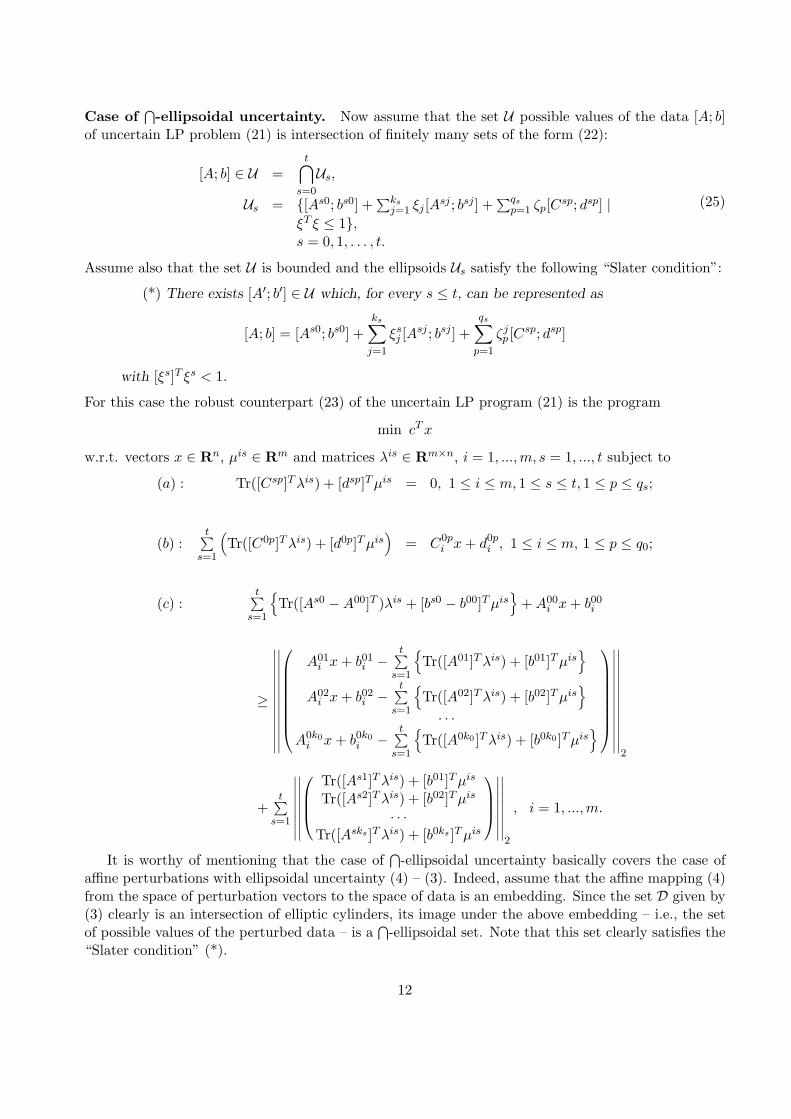
Case of⋂-ellipsoidal uncertainty. Now assume that the set U possible values of the data [A; b]
of uncertain LP problem (21) is intersection of finitely many sets of the form (22):
[A; b] ∈ U =t⋂
s=0
Us,
Us = {[As0; bs0] +∑ks
j=1 ξj [Asj ; bsj ] +∑qs
p=1 ζp[Csp; dsp] |ξT ξ ≤ 1},s = 0, 1, . . . , t.
(25)
Assume also that the set U is bounded and the ellipsoids Us satisfy the following “Slater condition”:
(*) There exists [A′; b′] ∈ U which, for every s ≤ t, can be represented as
[A; b] = [As0; bs0] +ks∑
j=1
ξsj [A
sj ; bsj ] +qs∑
p=1
ζjp [C
sp; dsp]
with [ξs]T ξs < 1.
For this case the robust counterpart (23) of the uncertain LP program (21) is the program
min cT x
w.r.t. vectors x ∈ Rn, µis ∈ Rm and matrices λis ∈ Rm×n, i = 1, ...,m, s = 1, ..., t subject to
(a) : Tr([Csp]T λis) + [dsp]T µis = 0, 1 ≤ i ≤ m, 1 ≤ s ≤ t, 1 ≤ p ≤ qs;
(b) :t∑
s=1
(Tr([C0p]T λis) + [d0p]T µis
)= C0p
i x + d0pi , 1 ≤ i ≤ m, 1 ≤ p ≤ q0;
(c) :t∑
s=1
{Tr([As0 −A00]T )λis + [bs0 − b00]T µis
}+ A00
i x + b00i
≥
∣∣∣∣∣∣∣∣∣∣∣∣∣
∣∣∣∣∣∣∣∣∣∣∣∣∣
A01i x + b01
i −t∑
s=1
{Tr([A01]T λis) + [b01]T µis
}
A02i x + b02
i −t∑
s=1
{Tr([A02]T λis) + [b02]T µis
}
· · ·A0k0
i x + b0k0i −
t∑s=1
{Tr([A0k0 ]T λis) + [b0k0 ]T µis
}
∣∣∣∣∣∣∣∣∣∣∣∣∣
∣∣∣∣∣∣∣∣∣∣∣∣∣2
+t∑
s=1
∣∣∣∣∣∣∣∣
∣∣∣∣∣∣∣∣
Tr([As1]T λis) + [b01]T µis
Tr([As2]T λis) + [b02]T µis
· · ·Tr([Asks ]T λis) + [b0ks ]T µis
∣∣∣∣∣∣∣∣
∣∣∣∣∣∣∣∣2
, i = 1, ..., m.
It is worthy of mentioning that the case of⋂
-ellipsoidal uncertainty basically covers the case ofaffine perturbations with ellipsoidal uncertainty (4) – (3). Indeed, assume that the affine mapping (4)from the space of perturbation vectors to the space of data is an embedding. Since the set D given by(3) clearly is an intersection of elliptic cylinders, its image under the above embedding – i.e., the setof possible values of the perturbed data – is a
⋂-ellipsoidal set. Note that this set clearly satisfies the
“Slater condition” (*).
12
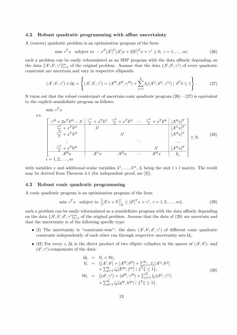
4.2 Robust quadratic programming with affine uncertainty
A (convex) quadratic problem is an optimization program of the form
min cT x subject to − xT [Ai]T [Ai]x + 2[bi]T x + γi ≥ 0, i = 1, . . . ,m; (26)
such a problem can be easily reformulated as an SDP program with the data affinely depending onthe data {Ai, bi, γi}m
i=1 of the original problem. Assume that the data (Ai, bi, γi) of every quadraticconstraint are uncertain and vary in respective ellipsoids:
(Ai, bi, γi) ∈ Ui =
(Ai, bi, γi) = (Ai0, bi0, γi0) +
k∑
j=1
δj(Aij , bij , γij) | δT δ ≤ 1
. (27)
It turns out that the robust counterpart of uncertain conic quadratic program (26) – (27) is equivalentto the explicit semidefinite program as follows:
min cT xs.t.
γi0 + 2xT bi0 − λi γi1
2 + xT bi1 γi2
2 + xT bi2 · · · γik
2 + xT bik [Ai0x]Tγi1
2 + xT bi1 λi [Ai1x]Tγi2
2 + xT bi2 λi [Ai2x]T...
. . . · · ·γik
2 + xT bik λi [Aikx]T
Ai0x Ai1x Ai2x · · · Aikx Ili
º 0,
i = 1, 2, . . . ,m
(28)
with variables x and additional scalar variables λ1, . . . , λm, Il being the unit l × l matrix. The resultmay be derived from Theorem 4.1 (for independent proof, see [3]).
4.3 Robust conic quadratic programming
A conic quadratic program is an optimization program of the form
min cT x subject to∣∣∣∣∣∣Aix + bi
∣∣∣∣∣∣2≤ [di]T x + γi, i = 1, 2, . . . ,m}. (29)
such a problem can be easily reformulated as a semidefinite program with the data affinely dependingon the data {Ai, bi, di, γi}m
i=1 of the original problem. Assume that the data of (29) are uncertain andthat the uncertainty is of the following specific type:
• (I) The uncertainty is “constraint-wise”: the data (Ai, bi, di, γi) of different conic quadraticconstraint independently of each other run through respective uncertainty sets Ui;
• (II) For every i, Ui is the direct product of two elliptic cylinders in the spaces of (Ai, bi)- and(di, γi)-components of the data:
Ui = Vi ×Wi,
Vi = {[Ai; bi] = [Ai0; bi0] +∑ki
j=1 ξj [Aij ; bij ]+
∑qip=1 ζp[Eip; f ip] | ξT ξ ≤ 1},
Wi = {(di, γi) = (di0, γi0) +∑k′i
j=1 ξj(dij , γij)
+∑q′i
p=1 ζp(gip, hip) | ξT ξ ≤ 1}.
(30)
13
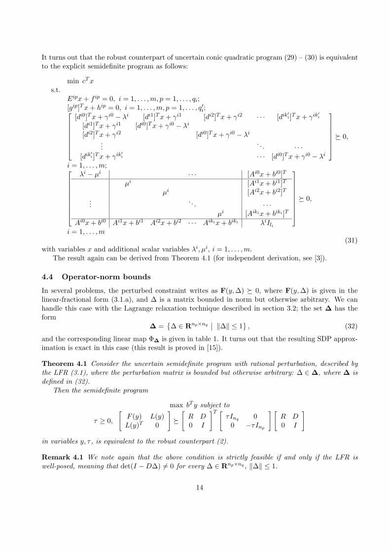
It turns out that the robust counterpart of uncertain conic quadratic program (29) – (30) is equivalentto the explicit semidefinite program as follows:
min cT xs.t.
Eipx + f ip = 0, i = 1, . . . , m, p = 1, . . . , qi;[gip]T x + hip = 0, i = 1, . . . ,m, p = 1, . . . , q′i;
[di0]T x + γi0 − λi [di1]T x + γi1 [di2]T x + γi2 · · · [dik′i ]T x + γik′i
[di1]T x + γi1 [di0]T x + γi0 − λi
[di2]T x + γi2 [di0]T x + γi0 − λi
.... . . · · ·
[dik′i ]T x + γik′i · · · [di0]T x + γi0 − λi
º 0,
i = 1, . . . , m;
λi − µi · · · [Ai0x + bi0]T
µi [Ai1x + bi1]T
µi [Ai2x + bi2]T...
. . . · · ·µi [Aikix + biki ]T
Ai0x + bi0 Ai1x + bi1 Ai2x + bi2 · · · Aikix + biki λiIli
º 0,
i = 1, . . . , m(31)
with variables x and additional scalar variables λi, µi, i = 1, . . . ,m.The result again can be derived from Theorem 4.1 (for independent derivation, see [3]).
4.4 Operator-norm bounds
In several problems, the perturbed constraint writes as F(y, ∆) º 0, where F(y, ∆) is given in thelinear-fractional form (3.1.a), and ∆ is a matrix bounded in norm but otherwise arbitrary. We canhandle this case with the Lagrange relaxation technique described in section 3.2; the set ∆ has theform
∆ ={∆ ∈ Rnp×nq
∣∣ ‖∆‖ ≤ 1}
, (32)
and the corresponding linear map Φ∆ is given in table 1. It turns out that the resulting SDP approx-imation is exact in this case (this result is proved in [15]).
Theorem 4.1 Consider the uncertain semidefinite program with rational perturbation, described bythe LFR (3.1), where the perturbation matrix is bounded but otherwise arbitrary: ∆ ∈ ∆, where ∆ isdefined in (32).
Then the semidefinite program
max bT y subject to
τ ≥ 0,
[F (y) L(y)L(y)T 0
]º
[R D0 I
]T [τInq 0
0 −τInp
] [R D0 I
]
in variables y, τ , is equivalent to the robust counterpart (2).
Remark 4.1 We note again that the above condition is strictly feasible if and only if the LFR iswell-posed, meaning that det(I −D∆) 6= 0 for every ∆ ∈ Rnp×nq , ‖∆‖ ≤ 1.
14
5 Examples
5.1 A link with combinatorial optimization
The method we have outlined is a way to solve a non convex optimization problem. It turns out thatthis method is similar in spirit to the one used in SDP relaxations for combinatorial optimization.
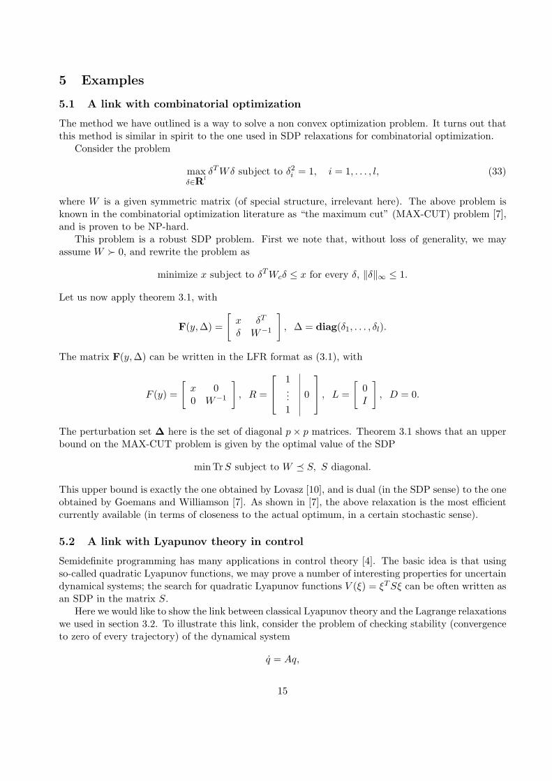
Consider the problem
maxδ∈Rl
δT Wδ subject to δ2i = 1, i = 1, . . . , l, (33)
where W is a given symmetric matrix (of special structure, irrelevant here). The above problem isknown in the combinatorial optimization literature as “the maximum cut” (MAX-CUT) problem [7],and is proven to be NP-hard.
This problem is a robust SDP problem. First we note that, without loss of generality, we mayassume W Â 0, and rewrite the problem as
minimize x subject to δT Wcδ ≤ x for every δ, ‖δ‖∞ ≤ 1.
Let us now apply theorem 3.1, with
F(y, ∆) =
[x δT
δ W−1
], ∆ = diag(δ1, . . . , δl).
The matrix F(y, ∆) can be written in the LFR format as (3.1), with
F (y) =
[x 00 W−1
], R =
1...1
0
, L =
[0I
], D = 0.
The perturbation set ∆ here is the set of diagonal p× p matrices. Theorem 3.1 shows that an upperbound on the MAX-CUT problem is given by the optimal value of the SDP
minTrS subject to W ¹ S, S diagonal.
This upper bound is exactly the one obtained by Lovasz [10], and is dual (in the SDP sense) to the oneobtained by Goemans and Williamson [7]. As shown in [7], the above relaxation is the most efficientcurrently available (in terms of closeness to the actual optimum, in a certain stochastic sense).
5.2 A link with Lyapunov theory in control
Semidefinite programming has many applications in control theory [4]. The basic idea is that usingso-called quadratic Lyapunov functions, we may prove a number of interesting properties for uncertaindynamical systems; the search for quadratic Lyapunov functions V (ξ) = ξT Sξ can be often written asan SDP in the matrix S.
Here we would like to show the link between classical Lyapunov theory and the Lagrange relaxationswe used in section 3.2. To illustrate this link, consider the problem of checking stability (convergenceto zero of every trajectory) of the dynamical system
q = Aq,
15
where q ∈ Rn is the state, and A is a (constant) square matrix. Taking the Laplace transform, weobtain that stability is equivalent to matrix A having no eigenvalues with positive real part:
(sI −A)H(sI −A) Â 0 for every s, s + s∗ ≥ 0.
The above is a robustness analysis problem (the Laplace variable s is the uncertainty). Introducep = sq, we have
p = sq for some s, s + s∗ ≥ 0
if and only if pqH + qpH º 0. Our problem is thus to check if
‖p−Aq‖2 > 0 for every (p, q) 6= (0, 0), pqH + qpH º 0.
Using Lagrange relaxation of the last matrix inequality constraint, we obtain a sufficient condition forstability: There exists a real matrix S such that
AT S + SA ≺ 0, S Â 0.
The above condition is the Lyapunov condition for stability that is well known in control (it turns outthat this condition is necessary and sufficient if A is known and constant). If S satisfies this inequality,the quadratic function V (ξ) = ξT Sξ can be interpreted as a Lypaunov function proving stability (thatis, V decreases along every trajectory). The above is easily extended to the case when the matrix Ais uncertain (see [4]).
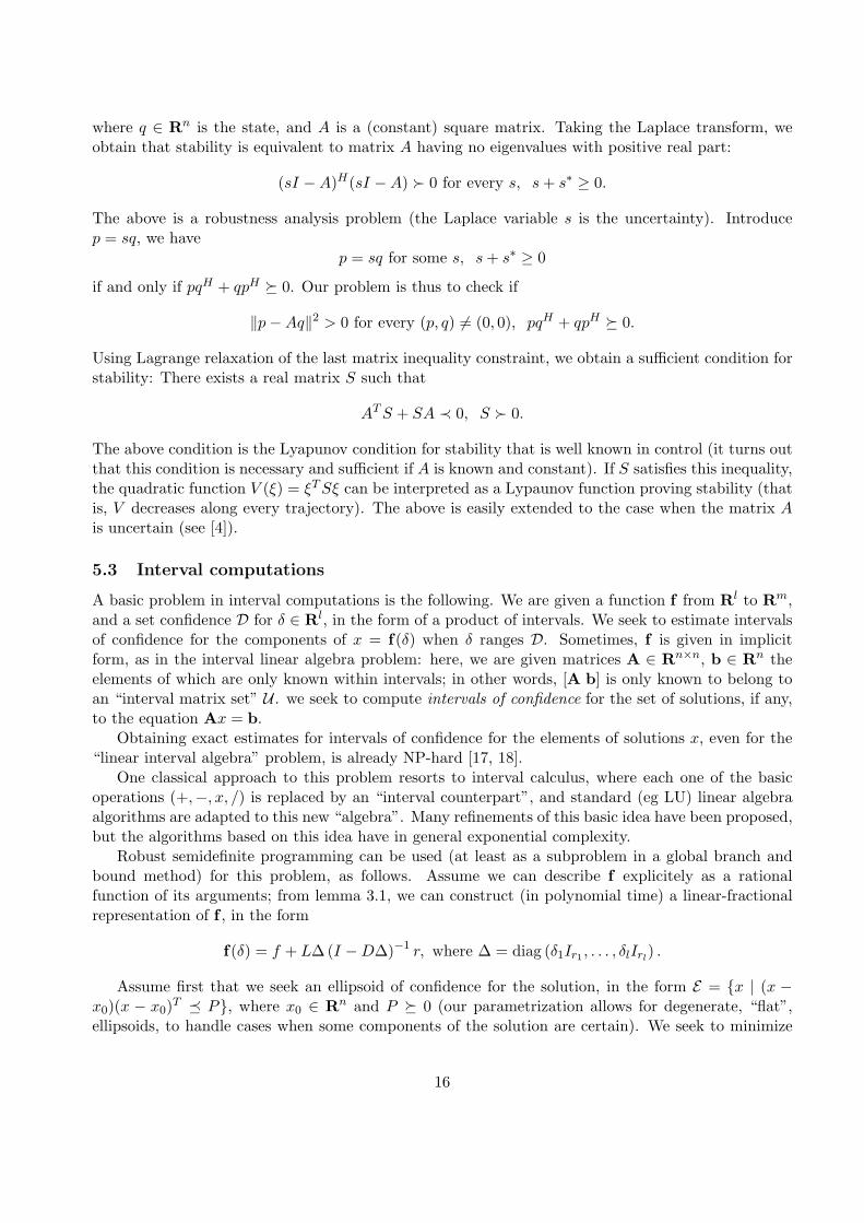
5.3 Interval computations
A basic problem in interval computations is the following. We are given a function f from Rl to Rm,and a set confidence D for δ ∈ Rl, in the form of a product of intervals. We seek to estimate intervalsof confidence for the components of x = f(δ) when δ ranges D. Sometimes, f is given in implicitform, as in the interval linear algebra problem: here, we are given matrices A ∈ Rn×n, b ∈ Rn theelements of which are only known within intervals; in other words, [A b] is only known to belong toan “interval matrix set” U . we seek to compute intervals of confidence for the set of solutions, if any,to the equation Ax = b.
Obtaining exact estimates for intervals of confidence for the elements of solutions x, even for the“linear interval algebra” problem, is already NP-hard [17, 18].
One classical approach to this problem resorts to interval calculus, where each one of the basicoperations (+,−, x, /) is replaced by an “interval counterpart”, and standard (eg LU) linear algebraalgorithms are adapted to this new “algebra”. Many refinements of this basic idea have been proposed,but the algorithms based on this idea have in general exponential complexity.
Robust semidefinite programming can be used (at least as a subproblem in a global branch andbound method) for this problem, as follows. Assume we can describe f explicitely as a rationalfunction of its arguments; from lemma 3.1, we can construct (in polynomial time) a linear-fractionalrepresentation of f , in the form
f(δ) = f + L∆ (I −D∆)−1 r, where ∆ = diag (δ1Ir1 , . . . , δlIrl) .
Assume first that we seek an ellipsoid of confidence for the solution, in the form E = {x | (x −x0)(x − x0)T ¹ P}, where x0 ∈ Rn and P º 0 (our parametrization allows for degenerate, “flat”,ellipsoids, to handle cases when some components of the solution are certain). We seek to minimize
16
the “size” of E subject to f(δ) ∈ E for every δ ∈ D. Measuring the size of E by TrP (other measuresare possible, as seen below), we obtain the following equivalent formulation of the problem.
minx0,P
TrP subject to
[P (f(δ)− x0)
(f(δ)− x0)T 1
]º 0 for every δ ∈ D. (34)
The above is obviously a robust semidefinite programming problem, for which an explicit SDP coun-terpart (approximation) can be devised, provided D takes the form of a (general) ellipsoidal set. (Atypical set arising in interval calculus is a product of intervals Π[δi δi], where δi, δi are given.)
The above method finds ellipsoids of confidence, but it is also possible to find intervals of confidencefor the components of f(δ), by modifying the objective of the above robust SDP suitably (for example,if we minimize the (1, 1) component of the matrix variable P instead of its trace, we will obtain aninterval of confidence for the first component of f(δ), when δ ranges D).
The resulting approximations have an interesting interpretation in the context of the “linear in-terval algebra problem” Ax = b, where [A b] is an uncertain matrix, subject to “unstructuredperturbations”. Assume
[A b] ∈ U = {[A + ∆A b + ∆b] | ‖[∆A ∆b]‖ ≤ ρ} ,
where [A b] ∈ Rn×(m+1) and ρ ≥ 0 are given. In this case, our results are exact, and yield a solutionrelated to the notion of total least squares developed by Golub and Van Loan [8, 21]. Precisely, it can beshown that the center of the ellipsoid of confidence (corresponding to the variable x0 in problem (34))is of the form
x0 = (AT A− ρ2I)−1AT b
(We assume that σmin([A b]) ≥ ρ, otherwise the ellipsoid of confidence is unbounded. Except in degen-erate cases, this guarantees the existence of the inverse in the above.) When we let ρ = σmin([A b]),the ellipsoid of confidence can be shown to be reduced to the singleton E = {x0}, and x0 is the “totalleast squares” solution to the problem Ax = b.
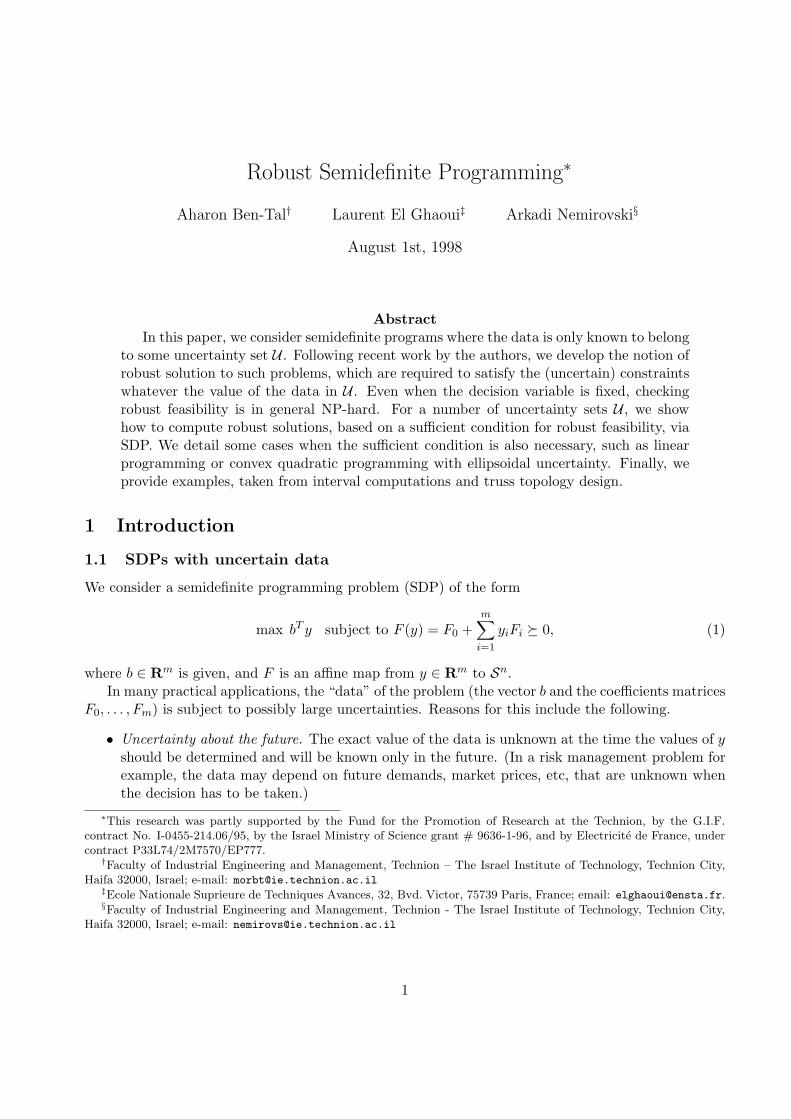
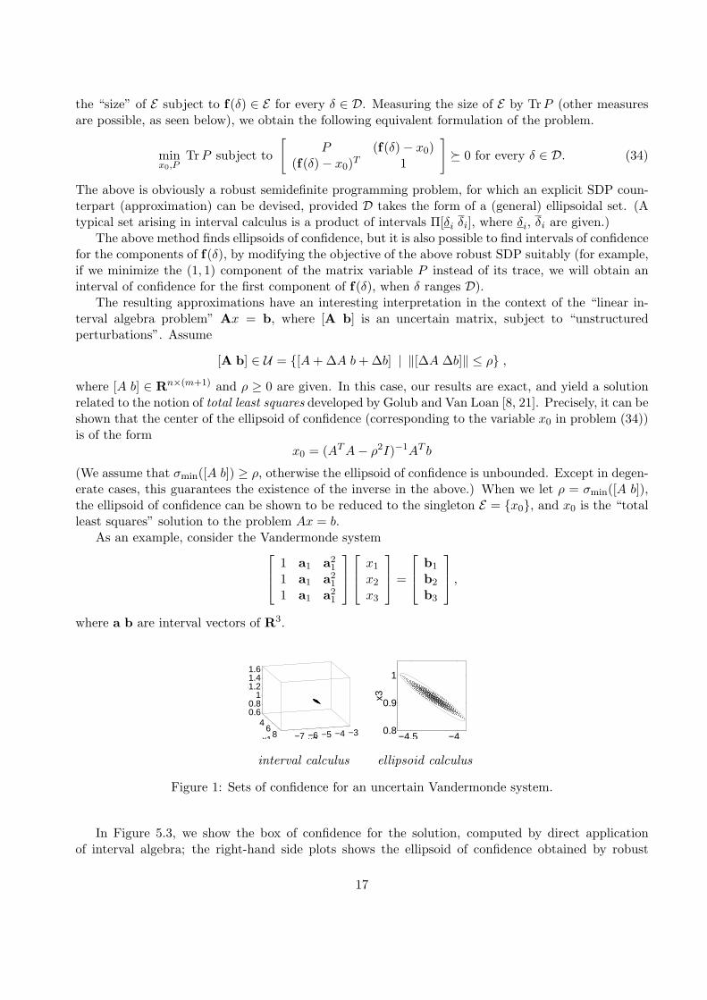
As an example, consider the Vandermonde system
1 a1 a21
1 a1 a21
1 a1 a21
x1
x2
x3
=
b1
b2
b3
,
where a b are interval vectors of R3.
46
8 −7 −6 −5 −4 −3
0.60.8
11.21.41.6
x2x1
x3
−4.5 −40.8
0.9
1
x2
x3
interval calculus ellipsoid calculus
Figure 1: Sets of confidence for an uncertain Vandermonde system.
In Figure 5.3, we show the box of confidence for the solution, computed by direct applicationof interval algebra; the right-hand side plots shows the ellipsoid of confidence obtained by robust
17
semidefinite programming. We did not use elaborate algorithms to solve the problem via intervalalgebra, so the reader should not draw negative conclusions about it; rather, the instructive part isthat the robust SDP method seems to behave well in this example.
5.4 Robust structural design
A typical problem of (static) structural design is to specify a mechanical construction capable best ofall withstand a given external load. As a concrete example of this type, consider the Truss TopologyDesign (TTD) problem (for more details, see [1]).
A truss is a construction comprised of thin elastic bars linked with each other at nodes – pointsfrom a given finite (planar or spatial) set. When subjected to a given load – a collection of externalforces acting at some specific nodes – the construction deformates, until the tensions caused by thedeformation compensate the external load. The deformated truss capacitates certain potential energy,and this energy – the compliance – measures stiffness of the truss (its ability to withstand the load);the less is compliance, the more rigid is the truss.
In the usual TTD problem we are given the initial nodal set, the external “nominal” load and thetotal volume of the bars. The goal is to allocate this resource to the bars in order to minimize thecompliance of the resulting truss. Mathematically the TTD problem can be modeled by the followingsemidefinite program:
min τs.t.
(a)
[τ fT
f∑n
i=1 tibibTi
]º 0,
(b) t ∈ P ⊂ Rn+,
(35)
with design variables τ ∈ R and t = (t1, . . . , tn) ∈ Rn; ti’s are volumes of tentative bars. The data ofthe problem are
• vectors bi ∈ Rm; they are readily given by the geometry of the nodal set;• vector f ∈ Rm representing the external load;• a polytope P representing design restrictions like upper bound on the total bar volume, bounds
on volumes of particular bars, etc.In reality, the external load f should be treated as uncertain element of the data; the traditional
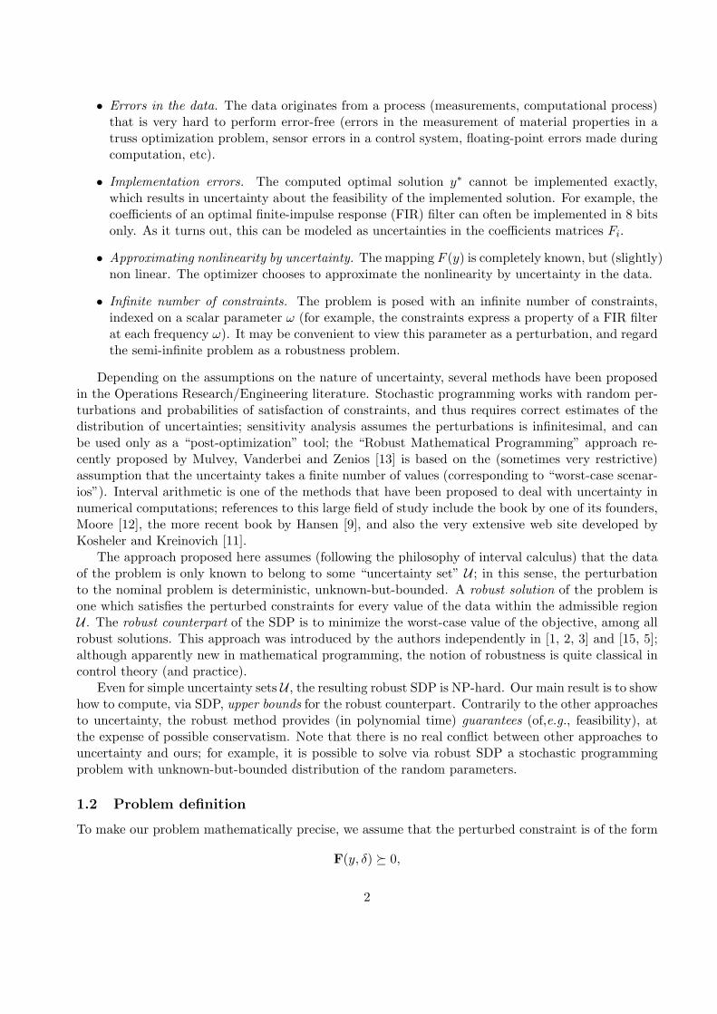
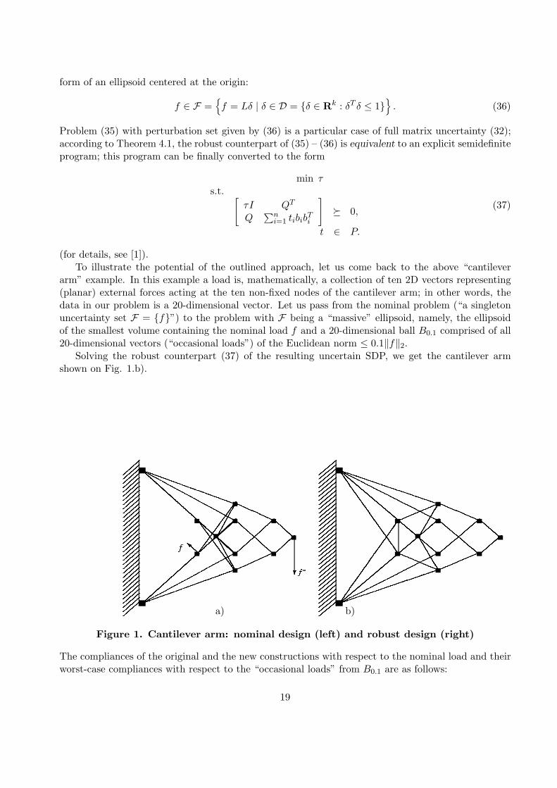
approach to treat this uncertainty is to consider a number of “loads of interest” f1, . . . , fk and tooptimize the worst-case, over this set of scenarios, compliance. Mathematically this approach isequivalent to replacing the LMI (35.a) (expressing the fact that τ is an upper bound on the compliancewith respect to f) by k similar constraints corresponding to f = f1, f = f2, . . . , f = fk. A disadvantageof the “scenario approach” is that it takes care just of a restricted number of “loads of interest” andignores “occasional” loads, even small ones; as a result, there is a risk that the resulting constructionwill be crushed by a small “bad” load. An example of this type is depicted on Fig. 1. Fig. 1.a) showsa cantilever arm which withstands optimally the nominal load – the unit force f∗ acting down at themost right node. The corresponding “nominal” optimal compliance is 1. It turns out, however, thatthe construction in question is highly instable: a small force f (10 times smaller than f∗) depictedby small arrow on Fig. 1.a) results in a compliance which is more than 3,000 times larger than thenominal one.
In order to improve design’s stability, it makes sense to treat the load as uncertain element of thedata varying through a “massive” uncertainty set rather than taking just a small number of “valuesof interest”. From the mathematical viewpoint, it is convenient to deal with uncertainty set in the
18
form of an ellipsoid centered at the origin:
f ∈ F ={f = Lδ | δ ∈ D = {δ ∈ Rk : δT δ ≤ 1}
}. (36)
Problem (35) with perturbation set given by (36) is a particular case of full matrix uncertainty (32);according to Theorem 4.1, the robust counterpart of (35) – (36) is equivalent to an explicit semidefiniteprogram; this program can be finally converted to the form
min τs.t. [
τI QT
Q∑n
i=1 tibibTi
]º 0,
t ∈ P.
(37)
(for details, see [1]).To illustrate the potential of the outlined approach, let us come back to the above “cantilever
arm” example. In this example a load is, mathematically, a collection of ten 2D vectors representing(planar) external forces acting at the ten non-fixed nodes of the cantilever arm; in other words, thedata in our problem is a 20-dimensional vector. Let us pass from the nominal problem (“a singletonuncertainty set F = {f}”) to the problem with F being a “massive” ellipsoid, namely, the ellipsoidof the smallest volume containing the nominal load f and a 20-dimensional ball B0.1 comprised of all20-dimensional vectors (“occasional loads”) of the Euclidean norm ≤ 0.1‖f‖2.
Solving the robust counterpart (37) of the resulting uncertain SDP, we get the cantilever armshown on Fig. 1.b).
�������������������������������������������������������������������� ������������
������������
�����
�����
������������
������������
���
���
������
����
����������
����������
������������
������������
�����
�������
�������
���
���
������
����
��������
���
���
���
���
���
��
��
��
��
��
��
��
��
��
��
��
��
��
��
��
��
��
��
��
��
��
��
��
��
��
��
��
��
��
��
��
��
� ������������
������������
�����
�����
������������
������������
���
���
������
����
������������
������������
�������
�������
�����
�����
���
���
������������
�����������������
�����
a) b)
Figure 1. Cantilever arm: nominal design (left) and robust design (right)
The compliances of the original and the new constructions with respect to the nominal load and theirworst-case compliances with respect to the “occasional loads” from B0.1 are as follows:
19
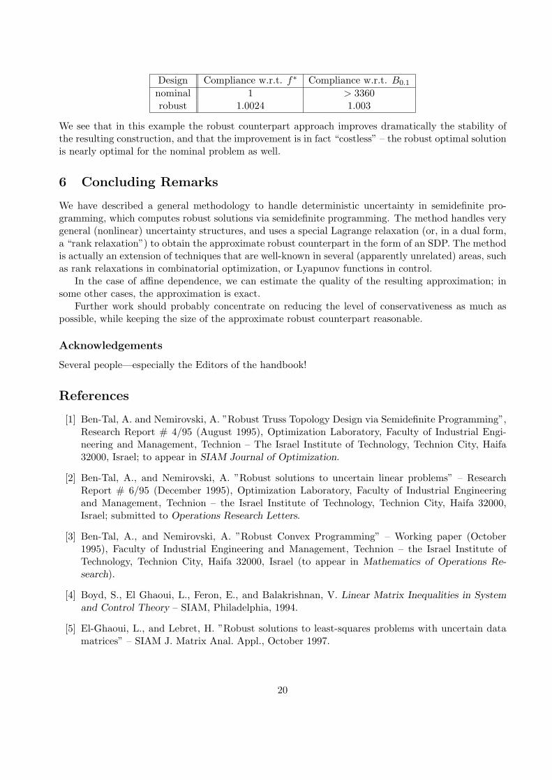
Design Compliance w.r.t. f∗ Compliance w.r.t. B0.1
nominal 1 > 3360robust 1.0024 1.003
We see that in this example the robust counterpart approach improves dramatically the stability ofthe resulting construction, and that the improvement is in fact “costless” – the robust optimal solutionis nearly optimal for the nominal problem as well.
6 Concluding Remarks
We have described a general methodology to handle deterministic uncertainty in semidefinite pro-gramming, which computes robust solutions via semidefinite programming. The method handles verygeneral (nonlinear) uncertainty structures, and uses a special Lagrange relaxation (or, in a dual form,a “rank relaxation”) to obtain the approximate robust counterpart in the form of an SDP. The methodis actually an extension of techniques that are well-known in several (apparently unrelated) areas, suchas rank relaxations in combinatorial optimization, or Lyapunov functions in control.
In the case of affine dependence, we can estimate the quality of the resulting approximation; insome other cases, the approximation is exact.
Further work should probably concentrate on reducing the level of conservativeness as much aspossible, while keeping the size of the approximate robust counterpart reasonable.
Acknowledgements
Several people—especially the Editors of the handbook!
References
[1] Ben-Tal, A. and Nemirovski, A. ”Robust Truss Topology Design via Semidefinite Programming”,Research Report # 4/95 (August 1995), Optimization Laboratory, Faculty of Industrial Engi-neering and Management, Technion – The Israel Institute of Technology, Technion City, Haifa32000, Israel; to appear in SIAM Journal of Optimization.
[2] Ben-Tal, A., and Nemirovski, A. ”Robust solutions to uncertain linear problems” – ResearchReport # 6/95 (December 1995), Optimization Laboratory, Faculty of Industrial Engineeringand Management, Technion – the Israel Institute of Technology, Technion City, Haifa 32000,Israel; submitted to Operations Research Letters.
[3] Ben-Tal, A., and Nemirovski, A. ”Robust Convex Programming” – Working paper (October1995), Faculty of Industrial Engineering and Management, Technion – the Israel Institute ofTechnology, Technion City, Haifa 32000, Israel (to appear in Mathematics of Operations Re-search).
[4] Boyd, S., El Ghaoui, L., Feron, E., and Balakrishnan, V. Linear Matrix Inequalities in Systemand Control Theory – SIAM, Philadelphia, 1994.
[5] El-Ghaoui, L., and Lebret, H. ”Robust solutions to least-squares problems with uncertain datamatrices” – SIAM J. Matrix Anal. Appl., October 1997.
20
[6] Falk, J.E. ”Exact Solutions to Inexact Linear Programs” – Operations Research (1976), pp.783-787.
[7] Goemans, M. X., and Williamson, D. P. ”.878-approximation for MAX CUT and MAX 2SAT”– In: Proc. 26th ACM Symp. Theor. Computing, 1994, pp. 422-431.
[8] Golub, G.H., and Van Loan, C.F. Matrix Computations. John Hopkins University Press, 1996.
[9] Hansen, E.R. Global optimization using interval analysis. Marcel Dekker, NY, 1992.
[10] Lovasz, L. ”On the Shannon capacity of a graph” – IEEE Transactions on Information Theoryv. 25 (1979), pp. 355-381.
[11] Kosheler, M., and Kreinovitch, V. Interval computations web sitehttp://cs.utep.edu/interval-comp/main.html, 1996.
[12] Moore, E.R. Methods and applications of interval analysis. SIAM, Philadelphia, 1979.
[13] Mulvey, J.M., Vanderbei, R.J. and Zenios, S.A. ”Robust optimization of large-scale systems”,Operations Research 43 (1995), 264-281.
[14] Nesterov, Yu., and Nemirovski, A. Interior point polynomial methods in Convex Programming,SIAM Series in Applied Mathematics, Philadelphia, 1994.
[15] Oustry, H., El Ghaoui, L., and Lebret, H. ”Robust solutions to uncertain semidefinite programs”,To appear in SIAM J. of Optimization, 1998.
[16] Rockafellar, R.T. Convex Analysis, Princeton University Press, 1970.
[17] Rohn, J. ”Systems of linear interval equations” – Linear Algebra and its Applications, v. 126(1989), pp. 39-78.
[18] Rohn, J. ”Overestimations in bounding solutions of perturbed linear equations” – Linear Algebraand its Applications, v. 262 (1997), pp. 55-66.
[19] Singh, C. ”Convex Programming with Set-Inclusive Constraints and its Applications to Gener-alized Linear and Fractional Programming” – Journal of Optimization Theory and Applications,v. 38 (1982), No. 1, pp. 33-42.
[20] Soyster, A.L. ”Convex Programming with Set-Inclusive Constraints and Applications to InexactLinear Programming” - Operations Research (1973), pp. 1154-1157.
[21] Van Huffel, S., and Vandewalle, J. The total least squares problem: computational aspects andanalysis. – v. 9 of Frontiers in applied Mathematics, SIAM, Philadelphia, 1991.
[22] Zhou, K., Doyle, J., and Glover, K. Robust and Optimal Control – Prentice Hall, New Jersey,1995.
21